Isometric deformations of wave fronts at non-degenerate singular points

Abstract.

Cuspidal edges and swallowtails are typical non-degenerate singular points on wave fronts in the Euclidean $3$-space. Their first fundamental forms belong to a class of positive semi-definite metrics called “Kossowski metrics”. A point where a Kossowski metric is not positive definite is called a singular point or a semi-definite point of the metric. Kossowski proved that real analytic Kossowski metric germs at their non-parabolic singular points (the definition of “non-parabolic singular point” is stated in the introduction here) can be realized as wave front germs (Kossowski’s realization theorem).

On the other hand, in a previous work with K. Saji, the third and the fourth authors introduced the notion of “coherent tangent bundle”. Moreover, the authors, with M. Hasegawa and K. Saji, proved that a Kossowski metric canonically induces an associated coherent tangent bundle.

In this paper, we shall explain Kossowski’s realization theorem from the viewpoint of coherent tangent bundles. Moreover, as refinements of it, we give a criterion that a given Kossowski metric can be realized as the induced metric of a germ of cuspidal edge (resp. swallowtail or cuspidal cross cap). Several applications of these criteria are given. Also, some remaining problems on isometric deformations of singularities of analytic maps are given at the end of this paper.

Introduction

Throughout this paper, we shall treat $C^{\infty}$-differentiable objects as well as real analytic ones. By the terminology “$C^{r}$-differentiable” we mean real analyticity if $r=\omega$ and $C^{\infty}$-differentiability if $r=\infty$.

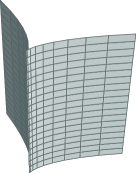
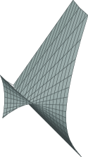
Figure 1. A cuspidal edge and a swallowtail.

We denote by $\boldsymbol{R}^{3}$ the Euclidean $3$-space. Let $M^{2}$ be a $C^{r}$-differentiable $2$-manifold and $f:M^{2}\to\boldsymbol{R}^{3}$ a $C^{r}$-map. A point $p\in M^{2}$ is called a singular point if $f$ is not an immersion at $p$. A singular point $p\in M^{2}$ is called a cuspidal edge (resp. swallowtail) if there exist a local $C^{r}$-coordinate system $(u,v)$ centered at $p$ and a local $C^{r}$-diffeomorphism $\Phi$ on $\boldsymbol{R}^{3}$ such that (cf. Figure 1)

(0.1) $$\Phi\circ f(u,v) =(u^{2},u^{3},v)\,(=:f_{\rm\tiny C}),$$

(0.2) $$(\mbox{resp.}\,\,\Phi\circ f(u,v) =(3u^{4}+u^{2}v,4u^{3}+2uv,v)(=:f_{\rm\tiny SW})).$$

A $C^{r}$-map $f:M^{2}\to\boldsymbol{R}^{3}$ is called a (co-orientable) frontal if there exists a $C^{r}$-differentiable unit vector field $\nu$ along $f$ such that $\nu(p)\in\boldsymbol{R}^{3}$ is perpendicular to $df(T_{p}M^{2})$ for each $p\in M^{2}$, where $T_{p}M^{2}$ is the tangent space of $M^{2}$ at $p$. Such a $\nu$ is called a unit normal vector field along $f$, and can be identified with the Gauss map

$$\nu:M^{2}\to S^{2}$$

by parallel transport in $\boldsymbol{R}^{3}$, where

(0.3) $$S^{2}:=\{(x,y,z)\in\boldsymbol{R}^{3}\,;\,x^{2}+y^{2}+z^{2}=1\}.$$

(The unit normal vector field $\nu$ can be chosen up to $\pm$-ambiguity at each local coordinate neighborhood, in general. The co-orientability of $f$ is the property that its unit normal vector field can be extended as a $C^{r}$-differentiable vector field along $f$. In this paper, we assume that frontals are all co-orientable.) A ($C^{r}$-differentiable) frontal $f$ is called a wave front if the induced map defined by

$$L:=(f,\nu):M^{2}\ni p\mapsto(f(p),\nu(p))\in\boldsymbol{R}^{3}\times S^{2}$$

is an immersion. It is well-known that cuspidal edges and swallowtails are typical singularities appearing on wave fronts. A singular point $p\in M^{2}$ of a $C^{r}$-map $f:M^{2}\to\boldsymbol{R}^{3}$ is called a cross cap (resp. a cuspidal cross cap) if there exist a local $C^{r}$-coordinate system $(u,v)$ and a local $C^{r}$-diffeomorphism $\Phi$ on $\boldsymbol{R}^{3}$ such that (cf. Figure 2)

(0.4) $$\Phi\circ f(u,v)=(u,uv,v^{2})(=:f_{\rm\tiny CR}),$$

(0.5) $$(\mbox{resp.}\,\,\,\Phi\circ f(u,v)=(u,v^{2},uv^{3})(=:f_{\rm\tiny CCR})).$$

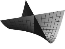
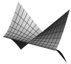
Figure 2. A cross cap and a cuspidal cross cap.

Cross caps are not frontals, since their unit normal vector fields cannot be extended continuously across the singular points. On the other hand, cuspidal cross caps are frontals, but not fronts.

Let $f:M^{2}\to\boldsymbol{R}^{3}$ be a $C^{r}$-frontal with $C^{r}$-differentiable unit normal vector field $\nu$. If we take a $C^{r}$-differentiable local coordinate system $(U;u,v)$ on $M^{2}$, then the function

(0.6) $$\lambda:=\det(f_{u},f_{v},\nu)\qquad(f_{u}:=\partial f/\partial u,~{}f_{v}:=\partial f/\partial v)$$

plays the role of an identifier of the singular points of $f$, that is, $\lambda(p)=0$ if and only if $p$ is a singular point. We call $\lambda$ the signed area density function on $U$. A singular point $p\in U$ (i.e. the point satisfying $\lambda(p)=0$) is said to be non-degenerate if the gradient vector $\nabla\lambda(p):=(\lambda_{u}(p),\lambda_{v}(p))$ does not vanish. If $p$ is a non-degenerate singular point, then, by the implicit function theorem, there exists a $C^{r}$-regular curve $\sigma(t)$ ($|t|<\varepsilon$) on $U$ parametrizing the singular set of $f$ such that $\sigma(0)=p$. We call the curve $\sigma$ the characteristic curve (or the singular curve) passing through $p$. Cuspidal edges, swallowtails and cuspidal cross caps are non-degenerate singular points.

Definition 1.

Let $p$ be a non-degenerate singular point of a $C^{r}$-frontal $f\colon{}M^{2}\to\boldsymbol{R}^{3}$. A $C^{r}$-differentiable local coordinate system $(U;u,v)$ centered at $p$ is called adjusted if $f_{v}(p)=\boldsymbol{0}$.

We denote by “$\cdot$” the canonical inner product on $\boldsymbol{R}^{3}$, and set $|\boldsymbol{a}|:=\sqrt{{\boldsymbol{a}}\cdot{\boldsymbol{a}}}$ ($\boldsymbol{a}\in\boldsymbol{R}^{3}$). Taking an adjusted coordinate system at a non-degenerate singular point $p$, we define

(0.7) $$\kappa_{\nu}(p):=\frac{{f_{uu}(p)}\cdot{\nu(p)}}{|f_{u}(p)|^{2}},$$

which is called the limiting normal curvature. The definition of $\kappa_{\nu}(p)$ does not depend on the choice of an adjusted coordinate system (cf. [11, (2.2)]).

Let $\gamma(t)$ be a curve on $M^{2}$ defined on an interval $I$ such that $\hat{\gamma}:=f\circ\gamma:I\to\boldsymbol{R}^{3}$ is a $C^{r}$-regular curve. Then the normal curvature function along $\hat{\gamma}$ is defined by

(0.8) $$\kappa_{n}(t):=\frac{{\hat{\gamma}^{\prime\prime}(t)}\cdot{\hat{\nu}(t)}}{|\hat{\gamma}^{\prime}(t)|^{2}}\qquad(\hat{\nu}:=\nu\circ\gamma),$$

where the prime ^′ means $d/dt$. We let $p$ be a non-degenerate singular point, and let $\sigma(t)$ ($|t|<\varepsilon$) be the characteristic curve passing through $p$ such that $p=\sigma(0)$. As shown in [11], the following assertion holds:

Fact 1.

If $p$ is a cuspidal edge or a cuspidal cross cap (resp. a swallowtail) on a $C^{r}$-differentiable frontal $f$, then $\hat{\sigma}(t):=f\circ\sigma(t)$ for $t\in I$ $($resp. for $t\in I\setminus\{0\})$ is a $C^{r}$-regular curve, and the value $\kappa_{\nu}(p)$ coincides with the normal curvature $\kappa_{n}(0)$ $($resp. the limit of the normal curvature $\displaystyle\lim_{t\to 0}\kappa_{n}(t))$.

Definition 2.

A non-degenerate singular point $p$ of a $C^{r}$-differentiable frontal $f$ is said to be $\nu$-flat if its limiting normal curvature $\kappa_{\nu}(p)$ vanishes, and is said to be non-$\nu$-flat otherwise.

Kossowski defined a class of positive semi-definite metrics on $2$-manifolds. We call metrics belonging to this class “Kossowski metrics” (see Definition 7). A point where a Kossowski metric is not positive definite is called a singular point or a semi-definite point of the metric. A Riemannian metric (i.e. a positive definite metric) is a Kossowski metric without singular points. (The concept of Kossowski metric can be generalized to manifolds of arbitrary dimension, see [17].)

In this paper, we consider singular points of metrics as well as singular points of $C^{r}$-differentiable maps. To distinguish between these two kinds of singular points, we use the terminology “semi-definite points” for singular points of a metric. On the other hand, a point where the metric is positive definite is called a regular point. A Kossowski metric on $M^{2}$ induces a $C^{r}$-function called a signed area density function (cf. (1.8)), which is defined on each coordinate neighborhood. The following fact explains how Kossowski metrics are related to frontals (see [8] and also [2]):

Fact 2.

The first fundamental form (i.e. the pull-back of the canonical metric on $\boldsymbol{R}^{3}$) of a $C^{r}$-differentiable frontal which admits only non-degenerate singular points is a $C^{r}$-differentiable Kossowski metric. Moreover, the signed area density function given in (0.6) coincides with that of the Kossowski metric up to $\pm$-multiple ambiguity.

Since this fact plays an important role, we shall prove this fact in Section 1. For each semi-definite point $p$ of a Kossowski metric, an invariant (cf. (1.13))

$$\Omega(p)\in T_{p}^{*}M^{2}\wedge T_{p}^{*}M^{2}$$

is defined. If $\Omega(p)=0$, we call $p$ a parabolic point of $ds^{2}$ (cf. Definition 9). The following fact explains the relationship between singular points on wave fronts and semi-definite points on Kossowski metrics.

Fact 3 ([11]).

Let $p$ be a non-degenerate singular point of a $C^{r}$-differentiable frontal $f:M^{2}\to\boldsymbol{R}^{3}$. Then the following three assertions are equivalent:

1. $p$ is a non-parabolic semi-definite point of the induced Kossowski metric,

2. $f$ is a wave front at $p$, and $p$ is a non-$\nu$-flat singular point of $f$,

3. $p$ is a regular point of the Gauss map of $f$.

Kossowski proved the following:

Fact 4 (Kossowski’s realization theorem [8]).

Let $ds^{2}$ be a real analytic (i.e. $C^{\omega}$-differentiable) Kossowski metric on a real analytic $2$-manifold $M^{2}$, and let $p\in M^{2}$ be a non-parabolic semi-definite point of $ds^{2}$. Then there exist a neighborhood $U$ of $p$ and a real analytic wave front $f:U\to\boldsymbol{R}^{3}$ such that the first fundamental form of $f$ coincides with $ds^{2}$ on $U$.

In a joint work with Saji [15], the third and the fourth authors introduced the notion of “coherent tangent bundle” and proved Gauss-Bonnet type formulas for it. A realization of the $C^{r}$-differentiable vector bundle as a limiting tangent bundle of a $C^{r}$-differentiable frontal is given in [16]. The purpose of this paper is to explain Kossowski’s realization theorem (Fact 4) from the viewpoint of the theory of coherent tangent bundles, and to prove several refinements. In fact, we define $A_{2}$ points and $A_{3}$ points as semi-definite points of a Kossowski metric $ds^{2}$ (see Definition 8). The following fact is important:

Fact 5 ([2, Proposition 2.19]).

Let $f:M^{2}\to\boldsymbol{R}^{3}$ be a $C^{r}$-differentiable wave front, and let $p\in M^{2}$ be a non-degenerate singular point. Then $p$ is a cuspidal edge $($resp. a swallowtail$)$ if and only if it is an $A_{2}$ semi-definite point (resp. an $A_{3}$ semi-definite point) of $ds^{2}$.

Cross caps are generic singular points appearing on $C^{\infty}$-differentiable maps of $2$-manifolds into $\boldsymbol{R}^{3}$. However, they never appear on frontals ([2, Proposition 4.3]). The corresponding assertion for cross cap singular points is an open problem (see Question 3 in Section 5).

If $p$ is an $A_{2}$ semi-definite point, then the secondary invariant

$$\Omega^{\prime}(p)\in T_{p}^{*}M^{2}\wedge T_{p}^{*}M^{2}$$

is also defined (cf. (1.18)). The following assertion holds:

Theorem A.

Let $M^{2}$ be a real analytic $2$-manifold and $ds^{2}$ a real analytic Kossowski metric on it. Suppose that $p\in M^{2}$ is a semi-definite point of the metric $ds^{2}$. Then there exists a real analytic frontal $f:U\to\boldsymbol{R}^{3}$ defined on a neighborhood $U$ of $p$ such that $ds^{2}$ is the first fundamental form of $f$, and the limiting normal curvature of $f$ at $p$ does not vanish. Moreover, such a realization $f$ satisfies the following properties:

1. $f$ is a wave front at $p$ if and only if $p$ is a non-parabolic point (of $ds^{2}$),

2. $f$ has a cuspidal edge at $p$ if and only if $p$ is a non-parabolic $A_{2}$ semi-definite point,

3. $f$ has a swallowtail at $p$ if and only if $p$ is a non-parabolic $A_{3}$ semi-definite point,

4. $f$ has a cuspidal cross cap at $p$ if and only if $p$ is a parabolic $A_{2}$ semi-definite point satisfying $\Omega^{\prime}(p)\neq 0$.

Fact 4 corresponds to the assertion (1). In particular, Theorem A is a generalization and refinement of Fact 4. We prove this in Section 4.

Remark 1.

Under the assumptions of Theorem A, it is shown in [6] that $f$ has a $5/2$-cuspidal edge at $p$ if the Gaussian curvature function $K$ of $ds^{2}$ can be extended as a smooth function defined on a sufficiently small neighborhood of $p$ and $dK(\eta)$ does not vanish at $p$, where $\eta\in T_{p}M^{2}$ is a null direction at the semi-definite point $p$.

Definition 3.

Let $f_{i}$ ($i=1,2$) be two germs of $C^{r}$-frontals. Then we say these two map germs are congruent (resp. isometric) if there exist an isometry germ $\Phi$ on $\boldsymbol{R}^{3}$ and a $C^{r}$-diffeomorphism germ $\varphi$ (resp. a $C^{r}$-diffeomorphism germ $\varphi$) such that $\Phi\circ f_{2}\circ\varphi=f_{1}$ (resp. $\varphi^{*}ds^{2}_{2}=ds^{2}_{1}$), where $ds^{2}_{i}$ ($i=1,2$) is the first fundamental form of $f_{i}$. On the other hand, two map germs are strongly congruent if there exists an isometry germ $\Phi$ on $\boldsymbol{R}^{3}$ such that $\Phi\circ f_{2}=f_{1}$.

The strong congruence implies the congruence. In this paper, we mainly discuss the number of strong congruence classes of wave fronts with the same first fundamental forms. The following theorem gives properties of the set of germs of real analytic frontals whose first fundamental forms coincide with a real analytic Kossowski metric germ $ds^{2}$ at $p\in M^{2}$.

Theorem B.

Let $M^{2}$ be a real analytic $2$-manifold and $ds^{2}$ a real analytic Kossowski metric on $M^{2}$. Let $\omega(t)$ and $\mu(t)$ be two germs of real analytic functions of one variable at $t=0$. For each $p\in M^{2}$, take a $C^{\omega}$-regular curve $\gamma(t)$ in $M^{2}$ such that $\gamma(0)=p$ and $\gamma^{\prime}(0)$ is not a null vector (i.e. $ds^{2}(\gamma^{\prime}(0),\gamma^{\prime}(0))>0$, see Definition 8). Then there exists a real analytic frontal germ $f=f_{\omega,\mu}$ satisfying the following properties:

1. $ds^{2}$ is the first fundamental form of $f$,

2. the normal curvature function germ along $\gamma$ defined by (0.8) coincides with $e^{\omega(t)}$ for a suitable choice of unit normal vector field $\nu$,

3. $\mu(t)$ gives the torsion function germ along $\hat{\gamma}(t)=f\circ\gamma(t)$,

4. if $p$ is a regular point $($resp. a non-parabolic semi-definite point$)$ of $ds^{2}$, then $f$ is an immersion $($resp. a wave front with non-vanishing limiting normal curvature$)$.

The possibilities for the strong congruence classes of such an $f$ are at most two. In particular, if $\mu$ vanishes identically $($i.e. $\hat{\gamma}$ is a planar curve$)$, then the strong congruence class of $f$ is uniquely determined.

Remark 2.

When $\gamma(t)$ is a characteristic curve of $ds^{2}$ consisting of semi-definite points of type $A_{2}$, the assertion of Theorem B is proved in [13]. So Theorem B can be considered as its generalization.

Remark 3.

In the last statement of Theorem B, we wrote that “the possibilities for the strong congruence classes of $f$ are at most two”. However, if we consider the possibilities for the congruence classes instead, the number turns to be “four” since we have the freedom to reverse the orientation of the singular curve, see [5] for details.

As a consequence, the following assertion holds:

Corollary C.

Let $I$ be an interval, and let $\{\omega_{s}(t)\}_{s\in I}$ and $\{\mu_{s}(t)\}_{s\in I}$ be two families of real analytic function germs of the variable $t$ depending real analytically on the parameter $s$. Then there exists a family $f_{s}:=f_{\omega_{s},\mu_{s}}$ $(s\in I)$ of real analytic frontal germs satisfying the properties $(1)$–$(4)$ in Theorem B for each $s\in I$ and depending on the parameter $s$ real analytically.

In Section 4, we prove Theorems A and B and Corollary C, and also give a variant (cf. Theorem 5) of Theorem B. When $p$ is an $A_{2}$ semi-definite point, we can choose $\gamma$ to be a characteristic curve, since $\gamma^{\prime}(0)$ is not a null vector. Then we obtain the following assertion:

Corollary D.

Let $f:(U,p)\to\boldsymbol{R}^{3}$ be a real analytic germ of cuspidal edge (resp. cuspidal cross cap), and let $\sigma(t)$ be a real analytic germ of regular curve in $U$ parametrizing the singular set by the arc-length parameter such that $\sigma(0)=p$. Suppose that the limiting normal curvature at $p$ does not vanish. We let $\Gamma(t)$ be a real analytic germ of regular space curve parametrized by the arc-length such that the curvature function $\kappa(t)$ of $\Gamma(t)$ is the same as that of $f\circ\sigma(t)$ $(\Gamma(t)$ may not have the same torsion function as $\hat{\sigma}(t):=f\circ\sigma(t))$. Then, for each choice of $\Gamma$, there exist a neighborhood $V(\subset U)$ of $p$ and a front $($resp. a frontal$)$ $g:(V,p)\to\boldsymbol{R}^{3}$ having a cuspidal edge (resp. cuspidal cross cap) at $p$ such that $g$ is isometric to $f$ and $\Gamma(t)=g\circ\sigma(t)$. Moreover, the possibilities for the strong congruence classes of such a $g$ are at most two.

We prove Corollary D also in Section 4. Here, we remark that, in [6], analogues of Theorems A and B and Corollary D are obtained for $5/2$-cuspidal edges. As a consequence of Theorem A and Theorem B, the following assertion is obtained:

Corollary E.

Let $f_{0}$, $f_{1}$ be two real analytic frontal germs with singularities whose limiting normal curvatures do not vanish. Suppose that they are mutually isometric. Then there exists a continuous deformation of real analytic frontal germs $g_{s}$ $(0\leq s\leq 1)$ satisfying the following properties:

1. $g_{0}=f_{0}$ and $g_{1}=f_{1}$,

2. $g_{s}$ is isometric to $g_{0}$,

3. the limiting normal curvature of each $g_{s}$ does not vanish.

Moreover, if both $f_{0}$ and $f_{1}$ are germs of cuspidal edges, swallowtails or cuspidal cross caps, then so are $g_{s}$ for $0\leq s\leq 1$.

In particular, if $T$ is an orientation reversing isometry of $\boldsymbol{R}^{3}$, then $T\circ f_{0}$ can be isometrically deformed into $f_{0}$ (see Remark 14 for details).

The paper is organized as follows: In Section 1, we recall the definition of Kossowski metrics, and define $A_{2}$ semi-definite points and $A_{3}$ semi-definite points. The relationship between frontals and the induced Kossowski metrics is also discussed there. In Section 2, we show the existence of certain orthogonal local coordinate systems (called “K-orthogonal coordinates”) for Kossowski metrics. Using this, we show representation formulas for $A_{2}$ or $A_{3}$ semi-definite points of Kossowski metrics. As an application, we also discuss properties of distance functions induced by Kossowski metrics. In Section 3, we explain the relationships between Kossowski metrics and their induced coherent tangent bundles. In Section 4, we prove the main results, using K-orthogonal coordinates. In Section 5, we mention some open questions relating to our results.

1. Kossowski metrics

Throughout this paper, we fix a $C^{r}$-differentiable $2$-manifold $M^{2}$, where $r=\infty$ or $\omega$. Let $ds^{2}$ be a positive semi-definite $C^{r}$-metric on $M^{2}$.

Definition 4.

A point $p\in M^{2}$ is called a regular point of $ds^{2}$ if $ds^{2}$ is positive definite at $p$, and is called a singular point or semi-definite point if it is not regular.

To distinguish from singular points of frontal maps, we use the terminology semi-definite points for singular points of semi-definite metrics. The set of semi-definite points in $M^{2}$ is called the semi-definite set.

For the sake of simplicity, we use the notations

(1.1) $$\partial_{u}:=\partial/\partial u,\qquad\partial_{v}:=\partial/\partial v$$

for each local coordinate system $(u,v)$ of $M^{2}$.

Definition 5.

Let $p$ be a semi-definite point of the metric $ds^{2}$ on $M^{2}$. Then a non-zero tangent vector $\boldsymbol{v}\in T_{p}M^{2}$ is called a null vector if

(1.2) $$ds^{2}(\boldsymbol{v},\boldsymbol{v})=0.$$

Moreover, a local coordinate neighborhood $(U;u,v)$ is called adjusted at $p\in U$ if $\partial_{v}$ gives a null vector of $ds^{2}$ at $p$.

It can be easily checked that (1.2) implies that $ds^{2}(\boldsymbol{v},\boldsymbol{x})=0$ holds for all $\boldsymbol{x}\in T_{p}M^{2}$. If $(U;u,v)$ is a local coordinate neighborhood adjusted at a semi-definite point $p=(0,0)$, then $F(0,0)=G(0,0)=0$ holds, where

(1.3) $$ds^{2}=E\,du^{2}+2F\,du\,dv+G\,dv^{2}.$$

We denote by $\mathcal{X}^{r}$ the set of $C^{r}$-differentiable vector fields on $M^{2}$, and by $C^{r}(M^{2})$ the set of real valued $C^{r}$-differentiable functions on $M^{2}$. We set $\langle{X},{Y}\rangle:=ds^{2}(X,Y)$ for $X,Y\in\mathcal{X}^{r}$. Kossowski [8] defined a map $\Theta:\mathcal{X}^{r}\times\mathcal{X}^{r}\times\mathcal{X}^{r}\to C^{r}(M^{2})$ as

(1.4) $$\Theta(X,Y,Z):=\frac{1}{2}\biggl{(}X\langle{Y},{Z}\rangle+Y\langle{X},{Z}\rangle-Z\langle{X},{Y}\rangle\\ +\langle{[X,Y]},{Z}\rangle-\langle{[X,Z]},{Y}\rangle-\langle{[Y,Z]},{X}\rangle\biggr{)},$$

where $[X,Y]:=XY-YX$. We call $\Theta$ the Kossowski pseudo-connection with respect to the Kossowski metric.

If the metric $ds^{2}$ is positive definite, then $\Theta(X,Y,Z)=\langle\nabla_{X}Y,Z\rangle$ holds, where $\nabla$ is the Levi-Civita connection of $ds^{2}$. One can easily check the following two identities (cf. [8])

(1.5) $$X\langle Y,Z\rangle=\Theta(X,Y,Z)+\Theta(X,Z,Y),$$

(1.6) $$\Theta(X,Y,Z)-\Theta(Y,X,Z)=\langle[X,Y],Z\rangle.$$

The equation (1.5) (resp. (1.6)) corresponds to the condition that $\nabla$ is a metric connection (resp. is torsion free). The following assertion can be also easily verified:

Proposition 1 (Kossowski [8]).

For each $Y\in\mathcal{X}^{r}$ and for each semi-definite point $p\in M^{2}$, the map

$$T_{p}M^{2}\times T_{p}M^{2}\ni(\boldsymbol{v}_{1},\boldsymbol{v}_{2})\longmapsto\Theta(V_{1},Y,V_{2})(p)\in\boldsymbol{R}$$

is a well-defined bilinear map, where $V_{j}$ $(j=1,2)$ are $C^{r}$-differentiable vector fields of $M^{2}$ satisfying $\boldsymbol{v}_{j}=V_{j}(p)$.

For each $p\in M^{2}$, the subspace

$$\mathcal{N}_{p}:=\biggl{\{}\boldsymbol{v}\in T_{p}M^{2}\,;\,ds^{2}(\boldsymbol{v},\boldsymbol{w})=0\mbox{ for all $\boldsymbol{w}\in T_{p}M^{2}$}\biggr{\}}$$

is called the null space or the radical of $ds^{2}$ at $p$. A non-zero vector belonging to $\mathcal{N}_{p}$ is a null vector at $p$ (cf. Definition 5).

Lemma 1 (Kossowski [8]).

Let $p$ be a semi-definite point of $ds^{2}$. Then the Kossowski pseudo-connection $\Theta$ induces a tri-linear map

$$\hat{\Theta}_{p}:T_{p}M^{2}\times T_{p}M^{2}\times\mathcal{N}_{p}\ni(\boldsymbol{v}_{1},\boldsymbol{v}_{2},\boldsymbol{v}_{3})\longmapsto\Theta(V_{1},V_{2},V_{3})(p)\in\boldsymbol{R},$$

where $V_{j}$ $(j=1,2,3)$ are $C^{r}$-vector fields of $M^{2}$ such that $\boldsymbol{v}_{j}=V_{j}(p)$.

Proof.

Applying (1.4),

$$2\Theta(V_{1},fV_{2},V_{3})$$

$$\phantom{aaa}=V_{1}\langle fV_{2},V_{3}\rangle+fV_{2}\langle V_{1},V_{3}\rangle-V_{3}\langle V_{1},fV_{2}\rangle$$

$$\phantom{aaaaaaaaa}+\langle[V_{1},fV_{2}],V_{3}\rangle-\langle[V_{1},V_{3}],fV_{2}\rangle-\langle[fV_{2},V_{3}],V_{1}\rangle$$

$$\phantom{aaa}=2f\Theta(V_{1},V_{2},V_{3})+(V_{1}f)\langle V_{2},V_{3}\rangle-(V_{3}f)\langle V_{1},V_{2}\rangle$$

$$\phantom{aaaaaaaaaaaaaaaaaaaaaaaaa}+(V_{1}f)\langle V_{2},V_{3}\rangle+(V_{3}f)\langle V_{2},V_{1}\rangle$$

$$\phantom{aaa}=2f\Theta(V_{1},V_{2},V_{3})+2(V_{1}f)\langle V_{2},V_{3}\rangle=2f\Theta(V_{1},V_{2},V_{3})$$

holds at $p$, where the fact that $V_{3}(p)\in\mathcal{N}_{p}$ is used to show the last equality. ∎

Definition 6.

A semi-definite point $p$ of the metric $ds^{2}$ is called admissible if $\hat{\Theta}_{p}$ in Lemma 1 vanishes.

A semi-definite point of the metric $ds^{2}$ is called of rank one if $\mathcal{N}_{p}$ is a $1$-dimensional subspace of $T_{p}M^{2}$.

By a suitable affine transformation in the $uv$-plane, one can take a local coordinate system adjusted at $p$ (cf. Definition 4). The following assertion gives a characterization of admissible semi-definite points:

Proposition 2 ([2]).

Let $(u,v)$ be a $C^{r}$-differentiable local coordinate system adjusted at a rank one semi-definite point $p$. Then $p$ is admissible if and only if

(1.7) $$F=G=0,\quad E_{v}=2F_{u},\quad G_{u}=G_{v}=0$$

hold at $p=(0,0)$, where $ds^{2}=E\,du^{2}+2F\,du\,dv+G\,dv^{2}$.

Proof.

Since $[\partial_{u},\partial_{v}]$ vanishes, and $\partial_{v}\in\mathcal{N}_{p}$ at $p$, the formula (1.4) yields that

$$2\hat{\Theta}(\partial_{u},\partial_{u},\partial_{v})=2\partial_{u}\langle\partial_{u},\partial_{v}\rangle-\partial_{v}\langle\partial_{u},\partial_{u}\rangle=2F_{u}-E_{v},$$

$$2\hat{\Theta}(\partial_{u},\partial_{v},\partial_{v})=\partial_{u}\langle\partial_{v},\partial_{v}\rangle+\partial_{v}\langle\partial_{u},\partial_{v}\rangle-\partial_{v}\langle\partial_{u},\partial_{v}\rangle=\partial_{u}\langle\partial_{v},\partial_{v}\rangle=G_{u},$$

$$2\hat{\Theta}(\partial_{v},\partial_{v},\partial_{v})=\partial_{v}\langle\partial_{v},\partial_{v}\rangle=G_{v}$$

hold at the origin $(0,0)$. Thus, $\hat{\Theta}_{p}$ vanishes if and only if (1.7) holds at $p$. ∎

Definition 7.

A $C^{r}$-differentiable positive semi-definite metric $ds^{2}$ is called a Kossowski metric if each semi-definite point $p\in M^{2}$ of $ds^{2}$ is admissible and there exists a $C^{r}$-function $\lambda(u,v)$ defined on a local coordinate neighborhood $(U;u,v)$ of $p$ such that

(1.8) $$EG-F^{2}=\lambda^{2}\qquad(\mbox{on $U$}),$$

(1.9) $$(\lambda_{u}(p),\lambda_{v}(p))\neq(0,0),$$

where $E,F,G$ are $C^{r}$-functions on $U$ satisfying (1.3).

We call such a $\lambda$ the signed area density function of $ds^{2}$ with respect to the local coordinate neighborhood $(U;u,v)$. In fact, if $ds^{2}$ is positive definite, then $dA:=|\lambda(u,v)|du\wedge dv$ gives the area element of the metric $ds^{2}$. The function $\lambda$ plays a role of an identifier of semi-definite points. In fact, $\lambda(p)=0$ if and only if $p$ is a semi-definite point. If $ds^{2}$ is the first fundamental form of a frontal $f:M^{2}\to\boldsymbol{R}^{3}$, then the function $\lambda$ given in (0.6) coincides with the signed area density function of $ds^{2}$.

As pointed out in the introduction (cf. Fact 2), the first fundamental form of a frontal $f:M^{2}\to\boldsymbol{R}^{3}$ whose singular points are all non-degenerate is a Kossowski metric.

Lemma 2.

We let $p$ be a semi-definite point of the Kossowski metric $ds^{2}$. Then the null space of $ds^{2}$ at $p$ is $1$-dimensional.

Proof.

Since $\lambda,F,G,G_{u}$ and $G_{v}$ vanish at $p$, twice differentiating the equality $EG-F^{2}=\lambda^{2}$ with respect to $u$ and $v$, we have

$$2\lambda_{u}(p)^{2}=E(p)G_{uu}(p)-2F_{u}(p)^{2},\qquad 2\lambda_{v}(p)^{2}=E(p)G_{vv}(p)-2F_{v}(p)^{2}.$$

If $E(p)=0$ then we have $\lambda_{u}(p)^{2}+F_{u}(p)^{2}=0$ and $\lambda_{v}(p)^{2}+F_{v}(p)^{2}=0$, which imply $(\lambda_{u}(p),\lambda_{v}(p))=(0,0)$ contradicting (1.9). So we have $E(p)\neq 0$, that is, $\partial_{u}$ is not a null vector. Thus, $\mathcal{N}_{p}$ is exactly $1$-dimensional, proving the assertion. ∎

By (1.9), we can apply the implicit function theorem for $\lambda(u,v)=0$, and find a $C^{r}$-regular curve $\sigma(t)$ $(|t|<\varepsilon)$ in the $uv$-plane (called the characteristic curve or the singular curve) parametrizing the semi-definite set of $ds^{2}$ such that $\sigma(0)=p$ and $\sigma:(-\varepsilon,\varepsilon)\to U$ is an embedding, where $\varepsilon$ is a sufficiently small positive number. The following assertion holds:

Proposition 3.

Let $ds^{2}$ be a $C^{r}$-differentiable Kossowski metric on $M^{2}$. We let $\lambda:U\to\boldsymbol{R}$ be a $C^{r}$-function satisfying (1.8) on a connected $C^{r}$-coordinate neighborhood $(U;u,v)$ of $M^{2}$. Then, the $2$-form

(1.10) $$d\hat{A}:=\lambda du\wedge dv$$

does not depend on the choice of such local coordinates, up to $\pm$-ambiguity, and gives a $C^{r}$-differentiable $2$-form defined on the universal covering of $M^{2}$.

Proof.

Let $(U;u,v)$ be a connected local coordinate neighborhood at $p$. Then $ds^{2}$ has the expression as in (1.3). Let $\lambda_{1},\lambda_{2}$ be two signed area density functions on $U$ satisfying $(\lambda_{1})^{2}=(\lambda_{2})^{2}=EG-F^{2}$. We fix $q\in U$ arbitrarily. If $q$ is a regular point, then $\lambda_{1}=\pm\lambda_{2}$ holds on a sufficiently small neighborhood of $W$ of $q$, obviously. So we suppose that $q\in U$ is a semi-definite point. Since we have observed that the semi-definite set around $q$ can be parametrized as a regular curve, we can take a new local coordinate system $(V;a,b)$ ($V\subset U$) centered at $q$ so that the $a$-axis is the characteristic curve. Then we have $\lambda_{1}(a,0)=\lambda_{2}(a,0)=0$. By the division lemma, there exist two $C^{r}$-function germs $\hat{\lambda}_{1}$, $\hat{\lambda}_{2}$ at $(0,0)$ such that

$$\lambda_{i}(a,b)=b\hat{\lambda}_{i}(a,b)\qquad(i=1,2)$$

on $V$. In particular, $(\lambda_{1})_{a}(0,0)=(\lambda_{2})_{a}(0,0)=0$ hold. By (1.9), we have that

$$0\neq(\lambda_{i})_{b}(0,0)=\hat{\lambda}_{i}(0,0)\qquad(i=1,2),$$

and $\varphi:=\lambda_{1}/\lambda_{2}=\hat{\lambda}_{1}/\hat{\lambda}_{2}$ gives a $C^{r}$-function defined on a connected neighborhood $W(\subset V)$ of the origin. Then we have

$$(\lambda_{2})^{2}=(\lambda_{1})^{2}=(\lambda_{2})^{2}\varphi^{2}.$$

Since $\lambda_{1}\neq 0$ except on the $a$-axis, $1=\varphi^{2}$ holds on $W$ by the continuity of $\varphi$, and that implies $\lambda_{1}=\pm\lambda_{2}$ on $W$. Since $U$ is connected and $q$ is arbitrarily fixed, $\lambda_{1}=\lambda_{2}$ or $\lambda_{1}=-\lambda_{2}$ holds on $U$. So we now set $\lambda:=\lambda_{1}$.

We next prove the second assertion. Let $(x,y)$ be another local coordinate system on $U$. Then

(1.11) $$\lambda du\wedge dv=\lambda(u_{x}dx+u_{y}dy)\wedge(v_{x}dx+v_{y}dy)=\lambda(u_{x}v_{y}-u_{y}v_{x})dx\wedge dy$$

holds on $U$. On the other hand, if we write $ds^{2}=\tilde{E}dx^{2}+2\tilde{F}dxdy+\tilde{G}dy^{2}$, then we have that

$$\tilde{\lambda}^{2}=\tilde{E}\tilde{G}-\tilde{F}^{2}=(EG-F^{2})(u_{x}v_{y}-u_{y}v_{x})^{2}=\lambda^{2}(u_{x}v_{y}-u_{y}v_{x})^{2},$$

and so $\pm\lambda(u_{x}v_{y}-u_{y}v_{x})$ gives the area density function with respect to the coordinate neighborhood $(U;x,y)$. Thus, (1.11) yields the last assertion. ∎

Remark 4.

The $2$-form $d\hat{A}$ on $U$ given in (1.10) is called a $($local$)$ signed area element. If $d\hat{A}$ is well-defined on $M^{2}$, that is, if it can be taken to be a $2$-form on $M^{2}$ so that its restriction to each local coordinate neighborhood $(U;u,v)$ gives a signed area element of $(U;u,v)$, then we say that $ds^{2}$ is co-orientable on $M^{2}$.

Let $p$ be a semi-definite point of a Kossowski metric $ds^{2}$, and let $\sigma(t)$ be the characteristic curve satisfying $\sigma(0)=p$. Then there exists a $C^{r}$-differentiable non-zero vector field $\eta(t)$ along $\sigma(t)$ which points in the null direction of the metric $ds^{2}$. We call $\eta(t)$ a null vector field along the characteristic curve $\sigma(t)$.

Definition 8.

A semi-definite point $p\in M^{2}$ of a Kossowski metric $ds^{2}$ is called an $A_{2}$ semi-definite point or semi-definite point of type $A_{2}$ if the derivative $\sigma^{\prime}(0)$ of the characteristic curve at $p$ is linearly independent of the null direction $\eta(0)$. A semi-definite point $p$ which is not of type $A_{2}$ is called an $A_{3}$ semi-definite point, or semi-definite point of type $A_{3}$ if

(1.12) $$\left.\frac{d}{dt}\right|_{t=0}\det\left(\sigma^{\prime}(t),\,\eta(t)\right)\neq 0.$$

Remark 5.

Cuspidal edges (resp. swallowtails) are called $A_{2}$-singularities (resp. $A_{3}$-singularities) of wave fronts. These points are corresponding to $A_{2}$ semi-definite points (resp. $A_{3}$ semi-definite points) with respect to the induced Kossowski metrics. The naming of $A_{i}$ $(i=2,3)$ points comes from this fact.

Remark 6.

We can extend the null vector field $\eta(t)$ to be a $C^{r}$-differentiable vector field $\tilde{\eta}$ defined on a neighborhood of $p$. Then it can be easily checked that $p$ is an $A_{2}$ semi-definite point (resp. an $A_{3}$ semi-definite point) if and only if

$$\lambda_{\tilde{\eta}}(p)\neq 0\qquad(\mbox{resp.\ }\lambda_{\tilde{\eta}}(p)=0\mbox{ and }\lambda_{\tilde{\eta}\tilde{\eta}}(p)\neq 0),$$

where $\lambda_{\tilde{\eta}}:=d\lambda(\tilde{\eta})$, and $\lambda_{\tilde{\eta}\tilde{\eta}}:=d\lambda_{\tilde{\eta}}(\tilde{\eta})$.

We denote by $\Sigma$ the semi-definite set of the Kossowski metric $ds^{2}$ in $M^{2}$ (cf. Definition 4). Let $K$ be the Gaussian curvature of $ds^{2}$ defined on $M^{2}\setminus\Sigma$. For each sufficiently small local coordinate system $(U;u,v)$, the signed area element $d\hat{A}$ is defined (cf. Proposition 3). Then a $2$-form

(1.13) $$\Omega:=K\,d\hat{A}$$

is defined on $U\setminus\Sigma$, which can be extended as a $C^{r}$-differentiable $2$-form on $U$ (cf. [8] and [2, Theorem 2.15]). We call $\Omega$ the (local) Euler form associated to $ds^{2}$ (on $U$). If $\Omega$ can be extended as a $C^{r}$-differentiable $2$-form to $M^{2}$, then the integral

$$\frac{1}{2\pi}\int_{M^{2}}\Omega$$

gives the Euler characteristic of the associated coherent tangent bundle induced by $ds^{2}$ when $M^{2}$ is compact and orientable. See [2, Proposition 3.3].

Definition 9.

A semi-definite point $p\in M^{2}$ of a Kossowski metric $ds^{2}$ is called parabolic (resp. non-parabolic) if the Euler form $\Omega$ vanishes (resp. does not vanish) at $p$.

To prove Fact 3, we prepare the following lemma:

Lemma 3.

Let $f:M^{2}\to\boldsymbol{R}^{3}$ be a $C^{r}$-differentiable frontal and $p\in M^{2}$ a non-degenerate singular point of $f$. Suppose that $p$ is a non-parabolic point with respect to the first fundamental form $ds^{2}$ of $f$, then $f$ is a wave front at $p$.

Proof.

We let $p$ be an $A_{2}$ semi-definite point of $ds^{2}$. As shown in [11, Page 261], we can take a local coordinate system $(U;u,v)$ centered at $p$ satisfying the following three properties:

1. the $u$-axis coincides with the singular set, and $|f_{u}|=1$ on the $u$-axis,

2. $f_{v}(u,0)=\boldsymbol{0}$ for each $u$,

3. $\{f_{u},f_{vv},\nu\}$ is an orthonormal frame along the $u$-axis.

Then, as shown in [11, Pages 262–263], there is a $C^{r}$-function $\hat{K}$ on $U$ such that

(1.14) $$\hat{K}(u,v)=vK(u,v)$$

on $U\setminus\{v=0\}$, where $K$ is the Gaussian curvature of $ds^{2}$. Let $\lambda(u,v)$ be the signed area density function on $U$. Since $\lambda(u,0)=0$, there exists a $C^{r}$-function $\hat{\lambda}$ such that $\lambda(u,v)=v\hat{\lambda}(u,v)$. Thus, the Euler form can be written as

$$\Omega=K\lambda du\wedge dv=\hat{K}\hat{\lambda}du\wedge dv.$$

The function $\hat{K}$ coincides with the same function as in [11, Page 263]. Since $\lambda(u,0)=0$, it holds that $\lambda_{u}(0,0)=0$. By (1.9), we have $\hat{\lambda}(0,0)=\lambda_{v}(0,0)\neq 0$. In [11], the cuspidal curvature $\kappa_{c}$ and the product curvature $\kappa_{\Pi}$ are defined, and we have the following (cf. [11, (3.26)])

(1.15) $$\kappa_{\Pi}(p)=\kappa_{\nu}(p)\kappa_{c}(p).$$

Moreover, by [11, (3.25)], $\hat{K}(p)\neq 0$ if and only if $\kappa_{\Pi}(p)\neq 0$. As shown in [11, Proposition 3.11], $\kappa_{c}(p)\neq 0$ if and only if $f$ is a wave front. Since $p$ is non-parabolic point, $\kappa_{\Pi}(p)\neq 0$. So $f$ is a wave front at $p$.

We next consider the case that $p$ is not an $A_{2}$ semi-definite point. As shown in [11, Page 267], we can take a local coordinate system $(U;u,v)$ centered at $p$ satisfying the following three properties:

• $f_{u}(0,0)=\boldsymbol{0}$,

• the $u$-axis is the singular set, and

• $|f_{v}(0,0)|=1$.

Using this coordinate system, the Euler form satisfies $\Omega=\hat{K}\hat{\lambda}du\wedge dv$, where $\hat{K}(u,v)=vK(u,v)$, $\hat{\lambda}$ is a $C^{r}$-function satisfying $\lambda(u,v)=v\hat{\lambda}(u,v)$ and $\hat{\lambda}(0,0)\neq 0$ (cf. [11, Page 270]). Moreover,

(1.16) $$\hat{K}(u,0)=\mu_{\Pi}(p)+O(u)$$

holds (cf. [11, (4.12)]), where the normalized cuspidal curvature $\mu_{c}(p)$ is defined at [11, (4.6)] and satisfies (cf. [11, (4.10)])

(1.17) $$\mu_{\Pi}(p)=\kappa_{\nu}(p)\mu_{c}(p).$$

As shown in [11, Proposition 4.2], $\mu_{c}(p)\neq 0$ if and only if $f$ is a wave front at $p$. Since $\kappa_{\nu}(p)\neq 0$, (1.16) and (1.17) yield that $\mu_{c}(p)\neq 0$ if and only if $\Omega(p)\neq 0$. So the fact that $p$ is a non-parabolic point implies that $f$ is a wave front at $p$. ∎

Proof of Fact 3.

We suppose (1). By Lemma 3, (1) implies that $f$ is a wave front. We first consider the case that $p$ is an $A_{2}$ semi-definite point. Moreover, since $p$ is non-parabolic, as seen in the proof of Lemma 3, $\kappa_{\Pi}(p)\neq 0$ holds. So $\kappa_{\Pi}(p)=\kappa_{\nu}(p)\kappa_{c}(p)$ implies $\kappa_{\nu}(p)\neq 0$. Therefore, we obtain (2). We next consider the case that $p$ is not an $A_{2}$ semi-definite point. Since $p$ is non-parabolic, we have $\hat{K}(p)\neq 0$. Then (1.16) yields that $\mu_{\Pi}(p)\neq 0$. As seen in the proof of Lemma 3, the fact that $f$ is a wave front at $p$ implies $\mu_{c}(p)\neq 0$, and so $\kappa_{\nu}(p)\neq 0$ by (1.17). Thus we obtain (2).

We next suppose (2). Then (3) follows from the equivalency of (2) and (3) in [11, Corollary C]. Finally, we suppose (3). Since $\nu$ is an immersion at $p$, $f$ is a wave front at $p$. Then the limiting normal curvature of $f$ at $p$ does not vanish. Then [11, Theorem A] implies that $\Omega(=Kd\hat{A})$ does not vanish at $p$. So, $p$ is non-parabolic, that is, (1) holds. ∎

Let $p$ be an $A_{2}$ semi-definite point of $ds^{2}$ and $\sigma(t)$ the characteristic curve such that $\sigma(0)=p$. Since $p$ is of type $A_{2}$, the velocity vector $\sigma^{\prime}(0)$ is not a null vector, and so we may assume that $t$ is an arc-length parameter of $\sigma$, that is, $ds^{2}(\sigma^{\prime}(t),\sigma^{\prime}(t))$ is identically equal to $1$. Then the $2$-form

(1.18) $$\Omega^{\prime}(p):=\left.\frac{d}{dt}\Omega_{\sigma(t)}\right|_{t=0}\in T^{*}_{p}M^{2}\wedge T^{*}_{p}M^{2}$$

is defined, which is called the derived Euler form at $p$ associated with $ds^{2}$. The following assertion is an analogue of Fact 5, but we do not assume that $f$ is a wave front:

Proposition 4.

Let $f:M^{2}\to\boldsymbol{R}^{3}$ be a $C^{r}$-frontal and $p$ its non-degenerate singular point where the limiting normal curvature does not vanish. Then

1. $f$ is a wave front at $p$ if and only if $p$ is non-parabolic (i.e. $\Omega(p)\neq 0$) with respect to the first fundamental form $ds^{2}$ of $f$,

2. $p$ is a cuspidal edge if and only if it is an $A_{2}$ semi-definite point and $\Omega(p)\neq 0$,

3. $p$ is a swallowtail if and only if it is an $A_{3}$ semi-definite point and $\Omega(p)\neq 0$,

4. $p$ is a cuspidal cross cap if and only if it is an $A_{2}$ semi-definite point, $\Omega(p)=0$ and $\Omega^{\prime}(p)\neq 0$.

Proof.

We use the same notations as in the proof of Lemma 3. The first assertion (o) follows from the equivalency of (1) and (2) of Fact 3. The assertions (i) and (ii) immediately follow from Fact 3 and Fact 5. We next prove (iii). Take an $A_{2}$ semi-definite point $p$. The conditions $\Omega(p)=0$ and $\Omega^{\prime}(p)\neq 0$ are equivalent to the conditions

(1.19) $$\hat{K}(0,0)=0\mbox{ and }\hat{K}_{u}(0,0)\neq 0.$$

Moreover, by [11, (3.25)], (1.19) is reduced to

(1.20) $$\kappa_{\Pi}(p)=0\mbox{ and }\kappa^{\prime}_{\Pi}(p)\neq 0,$$

where $\kappa_{\Pi}$ (resp. $\kappa^{\prime}_{\Pi}$) is the product curvature (resp. the derivative product curvature) for $A_{2}$ semi-definite points defined in [11]. In [11], the derivative cuspidal curvature $\kappa^{\prime}_{c}$ is also defined, and we have the following identity (cf. [11, (3.26)])

(1.21) $$\kappa^{\prime}_{\Pi}(p)=\kappa^{\prime}_{\nu}(p)\kappa_{c}(p)+\kappa_{\nu}(p)\kappa^{\prime}_{c}(p).$$

We let $\sigma(t)$ be a characteristic curve such that $\sigma(0)=p$ and denote by $\kappa_{\nu}(t)$ and $\kappa_{c}(t)$ the limiting normal curvature and the cuspidal curvature at $\sigma(t)$, respectively. Since $f$ has non-vanishing limiting normal curvature, $\kappa_{\nu}(0)\neq 0$ holds. By (1.15) and (1.21), the condition (1.20) is equivalent to the conditions

(1.22) $$\kappa_{c}(0)=0\,\,\mbox{ and }\,\,\kappa^{\prime}_{c}(0)\neq 0.$$

On the other hand, the function $\psi_{ccr}(t)$ defined in [11, Fact 2.4 (3)] satisfies the identity $\psi_{ccr}(t)=\kappa_{c}(t)$, as shown in the proof of [11, Proposition 3.11]. Since $\psi_{ccr}(0)=\kappa_{c}(0)$ and $\psi^{\prime}_{ccr}(0)=\kappa^{\prime}_{c}(0)$, (1.22) is equivalent to the criterion for cuspidal cross caps given in [11, Fact 2.4 (3)]. So we obtain (iii). ∎

Remark 7.

The assertion (iii) of Proposition 4 may not hold if we neglect the assumption that the limiting normal curvature of $f$ does not vanish. More precisely, there exists a map germ at a cuspidal edge singular point $p$ satisfying $\Omega(p)=0$ and $\Omega^{\prime}(p)\neq 0$: As shown in [10], any germs of cuspidal edges are congruent to

(1.23) $$f(u,v)=\biggl{(}u,a_{0}(u)+v^{2},b_{0}(u)u^{2}+b_{2}(u)uv^{2}+b_{3}(u,v)v^{3}\biggr{)},$$

where $b_{3}(0,0)\neq 0$. In this normal form, we set

$$a_{0}(u)=b_{2}(u)=0,\quad b_{3}(u,v)=\frac{1}{6},\quad b_{0}(u)=\frac{u}{2}.$$

Then we obtain a wave front $f(u,v)=\left(u,v^{2},{u^{3}}/2+{v^{3}}/6\right)$ having cuspidal edge singularity at $(0,0)$ such that

$$\kappa_{c}(0)=1,\quad\kappa^{\prime}_{c}(0)=0,\quad\kappa_{\nu}(0)=0,\quad\kappa^{\prime}_{\nu}(0)=3.$$

The product curvature $\kappa_{\Pi}(u)$ and the derivative product curvature $\kappa^{\prime}_{\Pi}(u)$ satisfy $\kappa_{\Pi}(0)=0$ and $\kappa^{\prime}_{\Pi}(0)=3$, which yield $\Omega(0,0)=0$, $\Omega^{\prime}(0,0)\neq 0$, as seen in the proof of Proposition 4.

Corollary 1.

Let $ds^{2}$ be a $C^{r}$-differentiable Kossowski metric $ds^{2}$, and let $p\in M^{2}$ be an $A_{2}$ semi-definite point of $ds^{2}$ satisfying $\Omega(p)=0$ and $\Omega^{\prime}(p)\neq 0$. Let $(U;u,v)$ be a local $C^{r}$-coordinate system centered at $p$ satisfying the properties (1)–(3) in the proof of Lemma 3. Then there exist positive constants $\varepsilon,\,\,\delta$ such that the sign of the Gaussian curvature function $K(u,v)$ satisfies

$$\operatorname{sign}K(u,v)=\operatorname{sign}(uv\hat{K}_{u}(0,0))\qquad((u,v)\in C_{\varepsilon,\delta}),$$

where $\hat{K}$ is the function defined in (1.14) and

$$C_{\varepsilon,\delta}:=\{(u,v)\in U\,;\,0<|v|<\delta|u|,\,\,|u|<\varepsilon\}.$$

Proof.

We can write

$$\hat{K}(u,v)=vK(u,v),\quad\hat{K}(u,v)=\hat{K}(u,0)+v\varphi(u,v),$$

where $\varphi(u,v)$ is a $C^{r}$-function at $p$. Moreover, by (1.19), we can write

$$\hat{K}(u,0)=u\psi(u)\qquad(\psi(0)=\hat{K}_{u}(0,0)\neq 0),$$

where $\psi(u)$ is a $C^{r}$-function defined for sufficiently small $|u|$. Without loss of generality, we may assume that $\varphi(u,v)$ and $\psi(u)$ are defined on a domain

$$W:=\{(u,v)\,;\,\mbox{$|u|<\varepsilon$ and $|v|<\varepsilon$}\},$$

where $\varepsilon$ is a sufficiently small positive number. Choosing $W$ so that $\overline{W}\subset U$, we have the expression $K(u,v)={u\psi(u)}/{v}+\varphi(u,v)$ on $W\setminus\{v\neq 0\}$. Since $\psi(0)\neq 0$ and $\varepsilon$ can be taken to be arbitrarily small, we may assume $|\psi(u)|>m\,(>0)$ and $|\varphi(u,v)|<\Delta$ hold on $\overline{W}$ for some constants $m,\Delta$. We set $\delta:=m/\Delta$. If $|u/v|>1/\delta$, we have

$$\left|\frac{u\psi(u)}{v}\right|>\frac{m}{\delta}=\Delta>|\varphi(u,v)|$$

on $C_{\varepsilon,\delta}$. So the sign of $K(u,v)$ on $C_{\varepsilon,\delta}$ is equal to that of ${u\psi(u)}/{v}$. ∎

2. Properties of Kossowski metrics

In this section, we show the existence of a certain orthogonal coordinate system, which will be applied to prove Theorems A and B. Using this, we also give a method to construct Kossowski metrics having $A_{2}$ semi-definite points and $A_{3}$ semi-definite points.

2.1. K-orthogonal coordinates

Definition 10.

Let $ds^{2}$ be a $C^{r}$-differentiable Kossowski metric on $M^{2}$, and take a point $p$ on $M^{2}$. (We also consider the case that $p$ is a regular point.) A local coordinate neighborhood $(U;u,v)$ centered at $p$ is called a K-orthogonal coordinate system if

1. $E=1$ holds along the $u$-axis,

2. $F=0$ on $U$, and

3. $E_{v}=0$ holds along the characteristic curve $\sigma$ (when $p$ is a semi-definite point),

where we set $ds^{2}=E\,du^{2}+2F\,du\,dv+G\,dv^{2}$ and (3) corresponds to the second condition of (1.7). In this situation, if we set $\rho:=\sqrt{E}$, then the metric $ds^{2}$ has the following expression

(2.1) $$ds^{2}=(\rho du)^{2}+\left(\frac{\lambda dv}{\rho}\right)^{2},\qquad\rho>0,\qquad\rho(u,0)=1,$$

where $\lambda$ is the signed area density function on $U$.

Since $F=G=0$ at a semi-definite point $p$, the following assertion trivially holds:

Proposition 5.

Let $\sigma(t)$ be a characteristic curve passing through a semi-definite point $p$ of $ds^{2}$ and $(u,v)$ a K-orthogonal coordinate system centered at $p$. Then $\partial_{v}$ belongs to $\mathcal{N}_{\sigma(t)}$ for each $t$. In particular, $\partial_{v}$ gives a null vector field along $\sigma$.

We shall apply the following lemma given in Kossowski [8] to prove our main theorem:

Lemma 4.

Let $ds^{2}$ be a $C^{r}$-differentiable Kossowski metric on $M^{2}$, and take a point $p$ on $M^{2}$. Let $\gamma$ be a $C^{r}$-regular curve passing through $p\,\,(=\gamma(0))$ such that $\gamma^{\prime}(0)$ is not a null vector of $ds^{2}$ on $M^{2}$ (when $p$ is a semi-definite point). Then there exists a $C^{r}$-local coordinate neighborhood $(U;u,v)$ satisfying the following properties:

1. the $u$-axis corresponds to the curve $\gamma$,

2. the $u$-curves are orthogonal to the $v$-curves with respect to $ds^{2}$,

3. $\partial_{v}$ points in the null direction at each semi-definite point on $U$,

4. if $ds^{2}$ and $\gamma$ are real analytic, then so is $(u,v)$.

Proof.

When $p$ is a regular point, we take a $C^{r}$-differentiable vector field $X_{2}$ on $U$ such that $X_{2}$ has no zeros on $U$. On the other hand, if $p$ is a semi-definite point, we define $X_{2}$ as follows: Let $\sigma$ be the characteristic curve passing through $p$. We take a null vector field $\eta$ along $\sigma$. We then extend $\eta$ as a $C^{r}$-differentiable vector field $\tilde{\eta}$ defined on a local coordinate neighborhood $(U;u,v)$ by replacing $U$ with a tubular neighborhood of $\sigma$ in the $uv$-plane. We set $X_{2}:=\tilde{\eta}$. Take a $C^{r}$-differentiable vector field $X_{1}$ on $U$ so that the curve $\gamma$ is an integral curve of $X_{1}$. Since $\gamma^{\prime}(0)$ is not a null vector, we may assume that the vector fields in the pair $(X_{1},X_{2})$ are linearly independent at each point on $U$. By [19, Lemma B.5.4], there exists a $C^{r}$-differentiable local coordinate system $(x,y)$ centered at $p$ such that $\partial_{x},\partial_{y}$ are proportional to $X_{1},X_{2}$, respectively, and the $x$-axis parametrizes $\gamma$. We next set

$$Y_{1}:=\partial_{x},\qquad Y_{2}:=-\tilde{F}\,\partial_{x}+\tilde{E}\,\partial_{y},$$

where $ds^{2}=\tilde{E}\,dx^{2}+2\tilde{F}\,dx\,dy+\tilde{G}\,dy^{2}$. Then $Y_{1}$, $Y_{2}$ are $C^{r}$-differentiable vector fields without zeros satisfying $ds^{2}(Y_{1},Y_{2})=0$. By [19, Lemma B.5.4] again, there exists a new $C^{r}$-differentiable local coordinate system $(\tilde{u},\tilde{v})$ centered at $p$ such that $\partial_{\tilde{u}},\partial_{\tilde{v}}$ are proportional to $Y_{1},Y_{2}$, respectively, and the $\tilde{u}$-axis parametrizes $\gamma$. (In fact, by the proof of [19, Lemma B.5.4], one can check that $(\tilde{u},\tilde{v})$ is real analytic whenever $(x,y)$ is.) Since $\tilde{u}$-axis corresponds to the $x$-axis and $Y_{2}$ is proportional to $\partial_{y}$ on the characteristic curve $\sigma$, we can conclude that $\partial_{\tilde{v}}$ gives a null vector field along $\sigma$. Hence, the coordinates $(\tilde{u},\tilde{v})$ are the desired ones. ∎

Lemma 5.

Let $ds^{2}$ be a $C^{r}$-differentiable Kossowski metric on $M^{2}$, and let $(U;u,v)$ be a $C^{r}$-local coordinate system such that

(2.2) $$ds^{2}=Edu^{2}+(\lambda^{2}/E)\,dv^{2}$$

and $E>0$ on $U$, where $\lambda$ is the signed area density function. Then the new $C^{r}$-local coordinate system $(\tilde{u},\tilde{v})$ defined by

(2.3) $$\tilde{u}:=\int_{0}^{u}\sqrt{E(t,0)}dt,\qquad\tilde{v}:=v$$

gives a K-orthogonal coordinate system on $U$.

Proof.

We can write

$$ds^{2}=\rho(u,v)^{2}(\sqrt{E(u,0)}du)^{2}+\tilde{\lambda}(u,v)^{2}\rho(u,v)^{-2}dv^{2},$$

where

$$\tilde{\lambda}(u,v):=\frac{\lambda(u,v)}{\sqrt{E(u,0)}},\qquad\rho(u,v):=\sqrt{\frac{E(u,v)}{E(u,0)}}.$$

By giving the new coordinate system $(\tilde{u},\tilde{v})$ as in (2.3), and replacing the notation $(\tilde{u},\tilde{v})$ and $\tilde{\lambda}$ by the original $(u,v)$ and $\lambda$, we obtain the expression (2.1). ∎

&

Figure 3. The coordinates $(u,v)$ at an $A_{2}$ semi-definite point (left) and an $A_{3}$ semi-definite point (right), where $\Sigma$ is the set of semi-definite points.

We now prove the following assertion:

Proposition 6.

Let $ds^{2}$ be a $C^{r}$-differentiable Kossowski metric on $M^{2}$, and let $\gamma$ be a regular curve passing through $p$ $(=\gamma(0))\in M^{2}$ so that $\gamma^{\prime}(0)$ is not a null vector when $p$ is a semi-definite point. Then there exists a $C^{r}$-differentiable K-orthogonal coordinate system $(U;u,v)$ centered at $p$ such that the $u$-axis corresponds to the curve $\gamma$. Moreover, if $p$ is an $A_{2}$ semi-definite point, then the $u$-axis can be taken as a characteristic curve (see Figure 2.1).

Proof.

By Lemma 4, there exists a $C^{r}$-differentiable orthogonal coordinate system $(u,v)$ centered at each point $p\in M^{2}$ such that the metric has the expression as in (2.2), and the $\tilde{u}$-axis parametrizes the curve $\gamma$. Then we can apply Lemma 5 for this coordinate system, and obtain the desired K-orthogonal coordinate system. If $p$ is an $A_{2}$ semi-definite point, then we can choose $\gamma$ to be the characteristic curve $\sigma$. In this case, the $u$-axis parametrizes $\sigma$. ∎

2.2. A representation formula for $A_{2}$ semi-definite points

In this subsection, we give a representation formula for $C^{r}$-differentiable Kossowski metric germs at $A_{2}$ semi-definite points. We fix an $A_{2}$ semi-definite point $p\in M^{2}$ of a $C^{r}$-differentiable Kossowski metric $ds^{2}$, and take a $C^{r}$-differentiable K-orthogonal coordinate system $(u,v)$ (cf. Proposition 6) centered at $p$ with the expression as in (2.1). We may assume the $u$-axis parametrizes the characteristic curve. We set $\omega(u,v):=\log\rho(u,v)$. Since $\rho(u,0)=1$, we have $\omega(u,0)=0$. So there exists a $C^{r}$-function $\omega_{1}(u,v)$ such that $\omega(u,v)=v\omega_{1}(u,v)$. So we can write

$$\rho(u,v)=\exp(v\omega_{1}(u,v)).$$

Since $p$ is of type $A_{2}$, we may assume that the $u$-axis parametrizes the semi-definite set. Since $\rho_{v}(u,0)=0$ holds (cf. (3) of Definition 10), we have that $\omega_{1}(u,0)=0$. So there exists a $C^{r}$-function germ $\omega_{2}(u,v)$ at the origin so that $\omega_{1}(u,v)=v\omega_{2}(u,v)$. In particular, $\rho(u,v)=e^{v^{2}\omega_{2}(u,v)}$ holds. Since the $u$-axis is the semi-definite set, we have $\lambda(u,0)=0$, and there exists a $C^{r}$-function germ $\hat{\lambda}(u,v)$ at the origin so that $\lambda(u,v)=v\hat{\lambda}(u,v)$. Since $(0,0)$ is non-degenerate, we may assume $\hat{\lambda}(0,0)>0$. We denote by $C^{r}_{0}(\boldsymbol{R}^{2})$ the set of germs of $C^{r}$-functions at $(0,0)$ on $\boldsymbol{R}^{2}$. Summarizing the above discussions, we obtain the following assertion.

Theorem 1.

Let $h(u,v)$ and $k(u,v)$ be two germs in $C^{r}_{0}(\boldsymbol{R}^{2})$. Then

$$ds^{2}:=\rho^{2}du^{2}+(\rho^{-1}\lambda)^{2}dv^{2}\qquad\left(\rho:=e^{v^{2}h(u,v)},\,\,\,\lambda:=ve^{k(u,v)}\right)$$

gives a $C^{r}$-differentiable Kossowski metric germ at an $A_{2}$ semi-definite point. Conversely, any $C^{r}$-differentiable Kossowski metric germ with $A_{2}$ semi-definite points is given in this manner. Moreover, the Euler form along the semi-definite set (i.e. the $u$-axis) is given by

(2.4) $$\Omega(u,0)=e^{-k(u,0)}\left(2h(u,0)k_{v}(u,0)-3h_{v}(u,0)\right)du\wedge dv.$$

Proof.

Let $d\tau^{2}$ be a Riemannian metric which is expressed as $d\tau^{2}=Edu^{2}+Gdv^{2}$. It is well-known that the Gaussian curvature $K$ of $d\tau^{2}$ is given by (cf. [19, §10])

(2.5) $$K=-\frac{1}{\hat{e}\hat{g}}\left(\left(\frac{\hat{g}_{u}}{\hat{e}}\right)_{\!\!u}+\left(\frac{\hat{e}_{v}}{\hat{g}}\right)_{\!\!v}\right),$$

where $\hat{e}:=\sqrt{E}$ and $\hat{g}:=\sqrt{G}$. Applying this formula for $ds^{2}$ at its regular points, we obtain (2.4). By continuity, (2.4) holds even at semi-definite points of $ds^{2}$. ∎

In [2, Proposition 2.29], we gave another representation formula for $A_{2}$ semi-definite points, which controls $E$, $G$ $(:=\lambda^{2}/E)$ but not $\rho$, $\lambda$.

2.3. A representation formula for $A_{3}$ semi-definite points

We next consider the case that $p=(0,0)$ is an $A_{3}$ semi-definite point of a Kossowski metric $ds^{2}$, with the expression as in (2.1). This case is not discussed in [2]. We set

$$\omega(u,v):=\log\rho(u,v).$$

Since $\rho=1$ on the $u$-axis, we have $\omega(u,0)=0$. Since $\partial_{v}$ gives the tangential direction of the characteristic curve at $(0,0)$ (cf. Figure 2.1, right), the characteristic curve can be expressed as the image of a certain graph $u=g(v)$ satisfying $g(0)=g^{\prime}(0)=0$. We set

$$\mu(v):=\det{\begin{pmatrix}g^{\prime}(v)&0\\ 1&1\end{pmatrix}}=g^{\prime}(v).$$

Since $p$ is of type $A_{3}$, (1.12) yields that $\mu(0)=0$ and $\mu^{\prime}(0)=g^{\prime\prime}(0)\neq 0$. Replacing $(u,v)$ by $(-u,v)$ if necessary, we may assume that $g^{\prime\prime}(0)>0$ without loss of generality. Then there exists a $C^{r}$-function $\hat{g}(v)$ ($\hat{g}(0)>0$) such that $g(v)=v^{2}\hat{g}(v)$. Take new coordinates $\tilde{u}:=u$ and $\tilde{v}:=v\sqrt{\hat{g}(v)}$, then the semi-definite set can be expressed as $\tilde{u}=\tilde{v}^{2}$. So, we may assume that the parabola $u=v^{2}$ gives the semi-definite set. Since $\omega_{v}(v^{2},v)=0$ (cf. (3) of Definition 10), we have $\omega_{v}(u,v)=(u-v^{2})a(u,v)$ ($a\in C^{r}_{0}(\boldsymbol{R}^{2})$). In particular, $\omega_{vv}(0,0)=0$ holds. Since $\omega(u,0)=0$, we have

$$\omega(u,v)=\int_{0}^{v}(u-w^{2})a(u,w)dw.$$

On the other hand, since $\lambda(v^{2},v)=0$ and $(0,0)$ is a non-degenerate semi-definite point, we can write $\lambda=(u-v^{2})\hat{\lambda}(u,v)$ $(\hat{\lambda}(0,0)\neq 0)$, where $\hat{\lambda}\in C^{r}_{0}(\boldsymbol{R}^{2})$. Thus, we obtain the following:

Theorem 2.

Let $h(u,v)$ and $k(u,v)$ be two germs in $C^{r}_{0}(\boldsymbol{R}^{2})$. Then

$$ds^{2}:=\rho^{2}du^{2}+(\rho^{-1}\lambda)^{2}dv^{2},$$

$$\quad\left(\rho(u,v):=\exp\left(\int_{0}^{v}(u-w^{2})h(u,w)dw\right),\,\,\lambda(u,v):=(u-v^{2})e^{k(u,v)}\right)$$

gives a $C^{r}$-differentiable Kossowski metric germ at an $A_{3}$ semi-definite point. Conversely, any $C^{r}$-differentiable Kossowski metric germ at $A_{3}$ semi-definite points is given in this manner. Moreover, the Euler form at the origin is given by

(2.6) $$\Omega(0,0)=\left[e^{-k(0,0)}\biggl{(}-h_{v}(0,0)+h(0,0)k_{v}(0,0)\biggr{)}-2e^{k(0,0)}k_{u}(0,0)\right]du\wedge dv.$$

The formula (2.6) can be proved using (2.4) and the fact $\omega_{vv}(0,0)=0$.

2.4. Distance functions associated with Kossowski metrics

As an application of the existence of K-orthogonal coordinates, we investigate properties of the distance functions induced by Kossowski metrics:

Definition 11.

Suppose that $M^{2}$ is connected. Let $ds^{2}$ be a Kossowski metric on $M^{2}$, and fix two points $p,q\in M^{2}$. We denote by $\mathcal{P}_{p,q}$ the set of piecewise smooth arcs combining two points $p$ and $q$, and set $d_{ds^{2}}(p,q):=\inf\{L_{ds^{2}}(\gamma)\,;\gamma\in\mathcal{P}_{p,q}\}$, where $L_{ds^{2}}(\gamma)$ is the length of the arc $\gamma\in\mathcal{P}_{p,q}$ with respect to $ds^{2}$, that is,

$$L_{ds^{2}}(\gamma):=\int_{\gamma}\sqrt{ds^{2}(\gamma^{\prime}(t),\gamma^{\prime}(t))}\,dt.$$

We call $d_{ds^{2}}:M^{2}\times M^{2}\to[0,\infty)$ the pre-distance function associated with $ds^{2}$.

Since $d_{ds^{2}}(x,y)$ is symmetric with respect to the variables $x$, $y$ and satisfies the triangle inequality by definition, it gives a distance function if and only if $d_{ds^{2}}(x,y)=0$ implies $x=y$.

Definition 12.

Let $ds^{2}$ be a Kossowski metric on $M^{2}$. A semi-definite point $p\in M^{2}$ is called a peak if there exists a neighborhood $U$ of $p$ such that the semi-definite points on $U\setminus\{p\}$ consists only of $A_{2}$ semi-definite points.

For example, $A_{2}$ or $A_{3}$ semi-definite points are peaks. On the other hand, $ds^{2}_{0}=du^{2}+u^{2}dv^{2}$ gives a Kossowski metric whose semi-definite set coincides with the $v$-axis. Each point of the $v$-axis is not a peak, since the null-direction $\partial_{v}$ gives the tangential direction of the $v$-axis as its characteristic curve.

Remark 8.

In [15], a “peak singularity” on wave fronts is defined. Suppose that $ds^{2}$ is the first fundamental form of a wave front $f$. Let $p\in M^{2}$ be a non-degenerate singular point of $f$. Then there exists a neighborhood $U$ of $p\in M^{2}$ such that the restriction of $ds^{2}$ on $U$ is a Kossowski metric. Moreover, $p$ is a peak with respect to $ds^{2}$ if and only if $p$ is at most non-degenerate peak singular point of $f$. This fact immediately follows from the definition of peaks of $f$.

We show the following assertion:

Theorem 3.

Let $ds^{2}$ be a $C^{r}$-differentiable Kossowski metric on $M^{2}$ whose semi-definite points consist only of peaks. Then the pre-distance function associated with $ds^{2}$ gives a distance function which is compatible with the topology of $M^{2}$.

We set

(2.7) $$B_{ds^{2}}(p,r):=\left\{q\in M^{2}\,;\,d_{ds^{2}}(p,q)<r\right\}\qquad(p\in M^{2},\,\,r>0).$$

To prove Theorem 3, we prepare the following four lemmas:

Lemma 6.

Let $ds^{2}$ be a $C^{r}$-differentiable Kossowski metric and $d\tau^{2}$ a $C^{\infty}$-differentiable Riemannian metric on $M^{2}$ such that $ds^{2}<d\tau^{2}$ on $M^{2}$ $($that is, $ds^{2}(\boldsymbol{v},\boldsymbol{v})<d\tau^{2}(\boldsymbol{v},\boldsymbol{v})$ holds for each $\boldsymbol{v}\,(\neq\boldsymbol{0}))$. Then there exists $\varepsilon>0$ such that

$$B_{d\tau^{2}}(p,r)\subset B_{ds^{2}}(p,r)$$

holds for $r\in(0,\varepsilon)$.

Proof.

Since $ds^{2}<d\tau^{2}$, $L_{ds^{2}}(\gamma)\leq L_{d\tau^{2}}(\gamma)$ holds for each path $\gamma\in\mathcal{P}_{p,q}$ between two points $p,q\in M^{2}$. So we obtain $d_{ds^{2}}(p,q)\leq d_{d\tau^{2}}(p,q)$ and

$$B_{d\tau^{2}}(p,r)=\{q\,;\,d_{d\tau^{2}}(p,q)<r\}\subset\{q\,;\,d_{ds^{2}}(p,q)<r\}=B_{ds^{2}}(p,r).$$

∎

Lemma 7.

Let $ds^{2}$ be a $C^{r}$-differentiable Kossowski metric on $M^{2}$ and $p\in M^{2}$ an $A_{2}$ semi-definite point. Suppose that $U$ is an open neighborhood of $p$. Then there exists $\delta>0$ such that $B_{ds^{2}}(p,\delta)\subset U$.

Proof.

We can take a K-orthogonal coordinate neighborhood $(V;u,v)$ centered at $p$ satisfying the following properties (cf. Theorem 1):

1. the closure $\overline{V}$ of $V$ is a subset of $U$,

2. there exist $C^{r}$-functions $E$ and $G$ on $\overline{V}$ such that $ds^{2}=E\,du^{2}+G\,dv^{2}$,

3. $E>0$ on $\overline{V}$,

4. the set of semi-definite points of $ds^{2}$ coincides with the $u$-axis.

We set $\Omega:=\{(u,v)\in V\,;\,|u|\leq\varepsilon_{1},\,\,|v|\leq\varepsilon_{2}\}$ for sufficiently small $\varepsilon_{i}$ ($i=1,2$) and

$$S:=\{(u,v)\in\Omega\,;\,|v|\geq\varepsilon_{2}/2\}.$$

Then

$$m_{1}:=\min_{\Omega}(\sqrt{E}),\qquad m_{2}:=\min_{S}(\sqrt{G})$$

are positive. Suppose $q=(u_{0},v_{0})$ lies on the boundary of $\Omega$, and take $\gamma\in\mathcal{P}_{p,q}$. If $|u_{0}|=\varepsilon_{1}$, the path $\gamma$ travels horizontally across the left or right half of $\Omega$, and so one can easily show that $L(\gamma)>m_{1}\varepsilon_{1}$. Similarly if $|v_{0}|=\varepsilon_{2}$ then $\gamma$ travels vertically across one of the closed rectangular sub-domains of $S$, and so $L(\gamma)>m_{2}\varepsilon_{2}/2$. Thus, if we set

$$m_{0}:=\min\biggl{(}m_{1}\varepsilon_{1},\,\,\frac{m_{2}\varepsilon_{2}}{2}\biggr{)},$$

then $B_{ds^{2}}(p,m_{0})\subset\Omega\subset U$, proving the assertion. ∎

Lemma 8.

Let $ds^{2}$ be a $C^{r}$-differentiable Kossowski metric on $M^{2}$ whose semi-definite points are all of type $A_{2}$. Then the pre-distance function associated with $ds^{2}$ gives a distance function which is compatible with the topology of $M^{2}$.

Proof.

We take two distinct points $p,q\in M^{2}$. To prove $d_{ds^{2}}$ is a distance function, it is sufficient to show that $p\neq q$ implies $d_{ds^{2}}(p,q)\neq 0$. Since $M^{2}$ is a Hausdorff space, we can take a local coordinate neighborhood $(U;u,v)$ of $p$ satisfying $q\not\in U$. By Lemma 7, there exists $r>0$ such that $B_{ds^{2}}(p,r)\subset U$. Then $d_{ds^{2}}(p,q)\geq r$ holds. So $d_{ds^{2}}$ is a distance function.

We next show that $d_{ds^{2}}$ is compatible with the topology of $M^{2}$. We fix a point $p$ of $M^{2}$ arbitrarily, and take a local coordinate neighborhood $(U;u,v)$ centered at $p$ so that $\overline{U}$ is compact. Let $d\tau^{2}$ be the canonical Euclidean metric on the $uv$-plane. Suppose that $p$ is a regular point of $ds^{2}$. Then it can be easily checked that for each $r>0$, there exists $r^{\prime}>0$ such that $B_{ds^{2}}(p,r^{\prime})$ (resp. $B_{d\tau^{2}}(p,r^{\prime})$) is a subset of $B_{d\tau^{2}}(p,r)$ (resp. $B_{ds^{2}}(p,r)$). So we consider the case that $p$ is a semi-definite point of $ds^{2}$. By Lemma 7, we have

$$B_{ds^{2}}(p,r)\subset U.$$

For sufficiently small $r>0$, we can take a positive constant $m$ such that $ds^{2}<m\,d\tau^{2}$ on $\overline{U}$. We set $M^{2}=U$ and apply Lemma 6. Then

$$B_{d\tau^{2}}(p,r/\sqrt{m})\subset B_{ds^{2}}(p,r)(\subset U)$$

holds for sufficiently small $r>0$. On the other hand, applying Lemma 7 again, there exists $r^{\prime}>0$ such that $B_{ds^{2}}(p,r^{\prime})\subset B_{d\tau^{2}}(p,r)$. Thus, the topology induced by $d_{ds^{2}}$ is the same as that of $M^{2}$ as a manifold. ∎

Lemma 9.

Let $ds^{2}$ be a $C^{r}$-differentiable Kossowski metric on $M^{2}$, and let $p\in M^{2}$ be a peak. Suppose that $U$ is an open neighborhood of $p$. Then there exists $\delta>0$ such that $B_{ds^{2}}(p,\delta)\subset U$.

Proof.

We can take a local coordinate neighborhood $(V;u,v)$ centered at $p$ such that the closure $\overline{V}$ of $V$ is a subset of $U$. Take a sufficiently small $\varepsilon>0$, and set

$$\Omega:=\{q\in V\,;\,|q|\leq\varepsilon\},$$

where $|(u,v)|:=\sqrt{u^{2}+v^{2}}$. Consider the subset $S$ of $\Omega$ defined by

$$S:=\{q\in\Omega\,;\,|q|\geq\varepsilon/2\},$$

and set

$$m:=\inf\{d_{ds^{2}}(q_{1},q_{2})\,;\,|q_{1}|=\varepsilon,\,\,|q_{2}|=\varepsilon/2\}.$$

Since $U\setminus\{q\in\Omega\,;\,|q|\leq\varepsilon/3\}$ admits only regular points or $A_{2}$ semi-definite points, Lemma 8 yields that $m>0$. Suppose that $q=(u_{0},v_{0})$ lies on the boundary of $\Omega$, and take $\gamma\in\mathcal{P}_{p,q}$. Since the path $\gamma$ travels across $S$, we have $L_{ds^{2}}(\gamma)>m$. Thus, we have $B_{ds^{2}}(p,m)\subset\Omega\subset U$, proving the assertion. ∎

Proof of Theorem 3.

If we use Lemma 9 instead of Lemma 7, the same argument as in the proof of Lemma 8 gives the proof of Theorem 3. ∎

3. Coherent tangent bundles induced by Kossowski metrics

In this section, we deduce the partial differential equation given in Kossowski [8], using the fact (shown in [2]) that a Kossowski metric induces an associated vector bundle with a metric and a connection, called a “coherent tangent bundle”.

3.1. Fundamental theorem for frontals

Let $\mathcal{E}$ be a vector bundle of rank $2$ over a $2$-manifold $M^{2}$, and $\langle{\,},{\,}\rangle$ an inner product on $\mathcal{E}$. We let $\nabla$ be a connection on $\mathcal{E}$ which is compatible with respect to the inner product. If a vector bundle homomorphism $\varphi:TM^{2}\to\mathcal{E}$ which induces the identity map on $M^{2}$ satisfies the identity

(3.1) $$\nabla_{X}\varphi(Y)-\nabla_{Y}\varphi(X)=\varphi([X,Y])\qquad(X,Y\in\mathcal{X}^{r}),$$

then we call $(\mathcal{E},\langle{\,},{\,}\rangle,\nabla,\varphi)$ a coherent tangent bundle over $M^{2}$, where $\mathcal{X}^{r}$ is the set of $C^{r}$-vector fields on $M^{2}$. (This definition can be generalized for $n$-dimensional manifolds, cf. [17].) In this situation, the pull-back metric of $\langle{\,},{\,}\rangle$ via $\varphi$,

$$ds^{2}:=\varphi^{*}\langle{\,},{\,}\rangle$$

is induced, which is called the first fundamental form of $\varphi$. A point $p$ where $\varphi_{p}:T_{p}M^{2}\to\mathcal{E}_{p}$ has a non-trivial kernel corresponds to a semi-definite point of $ds^{2}$.

Definition 13.

Two coherent tangent bundles on $M^{2}$

$$(\mathcal{E}_{1},\langle{~{}},{~{}}\rangle_{1},\nabla^{1},\varphi_{1}),\qquad(\mathcal{E}_{2},\langle{~{}},{~{}}\rangle_{2},\nabla^{2},\varphi_{2})$$

are said to be isomorphic if there exists a bundle isomorphism $\iota\colon{}\mathcal{E}_{1}\to\mathcal{E}_{2}$ satisfying the following three conditions:

• $\varphi_{2}=\iota\circ\varphi_{1}$,

• $\iota$ preserves the inner products, that is, for each $p\in M^{2}$ and for each $\xi$, $\eta\in(\mathcal{E}_{1})_{p}$, $\langle{\xi},{\eta}\rangle_{1}=\langle{\iota(\xi)},{\iota(\eta)}\rangle_{2}$ holds,

• for each $\boldsymbol{v}\in T_{p}M^{2}$ and for each section $\xi$ of $\mathcal{E}_{1}$, $\iota(\nabla^{1}_{\boldsymbol{v}}\xi)=\nabla^{2}_{\boldsymbol{v}}\iota(\xi)$ holds.

In this situation, $\iota$ is called an isomorphism between coherent tangent bundles.

The following assertion holds:

Fact 6 ([2, Theorem 3.1]).

Let $M^{2}$ be an oriented $C^{\omega}$-differentiable $2$-manifold and $ds^{2}$ a $C^{\omega}$-differentiable Kossowski metric on $M^{2}$. Then there exists a unique $C^{\omega}$-differentiable coherent tangent bundle $(\mathcal{E},\langle{\,},{\,}\rangle,\,\nabla,\varphi)$ up to isomorphisms of coherent tangent bundles such that the induced metric $\varphi^{*}\langle{\,},{\,}\rangle$ coincides with $ds^{2}$. Moreover, $\mathcal{E}$ is orientable if and only if $ds^{2}$ is co-orientable (see Remark 4).

Remark 9.

$\mathcal{E}:=TM^{2}$ can be considered as a coherent tangent bundle if $\langle{\,},{\,}\rangle$ is a Riemannian metric, $\varphi$ is the identity map, and $\nabla$ is the Levi-Civita connection.

Remark 10.

Fact 6 was applied in [2] to prove two Gauss-Bonnet type formulas for Kossowski metrics. Moreover, Kossowski metrics can be defined on higher dimensional manifolds, and this fact was generalized for arbitrary dimension (see [17, Theorem 7.9]).

Definition 14 (Frontal bundles).

Suppose that there are two bundle homomorphisms $\varphi,\,\psi:TM^{2}\rightarrow(\mathcal{E},\langle{\,},{\,}\rangle,\nabla)$ such that each of them induces a structure of a coherent tangent bundle on $(\mathcal{E},\langle{\,},{\,}\rangle,\nabla)$. If they satisfy the following compatibility condition

(3.2) $$\langle{\varphi(X)},{\psi(Y)}\rangle=\langle{\varphi(Y)},{\psi(X)}\rangle\qquad(X,Y\in\mathcal{X}^{r}),$$

then $(\mathcal{E},\langle{\,},{\,}\rangle,\nabla,\varphi,\psi)$ is called a frontal bundle.

Example 1.

Let $f:M^{2}\to\boldsymbol{R}^{3}$ be a frontal, and let $\nu:M^{2}\to S^{2}$ be its unit normal vector field. Then

$$\mathcal{E}_{f}:=\{(p,\boldsymbol{w})\in M^{2}\times T\boldsymbol{R}^{3}\,;\,\mbox{$\boldsymbol{w}\in T_{p}\boldsymbol{R}^{3}$ is perpendicular to $\nu_{p}$}\}$$

has a structure of a vector bundle of rank $2$ over $M^{2}$. The inner product $\langle{\,},{\,}\rangle$ is induced from the canonical inner product of $\boldsymbol{R}^{3}$. Moreover, taking the tangential component of the Levi-Civita connection of $\boldsymbol{R}^{3}$, $\mathcal{E}_{f}$ has a connection $\nabla^{f}$ which is compatible with the metric $\langle{\,},{\,}\rangle$. Then the two bundle homomorphisms defined by

$$\varphi_{f}:TM^{2}\ni\boldsymbol{v}\mapsto(\pi(\boldsymbol{v}),df(\boldsymbol{v}))\in\mathcal{E}_{f}$$

and

$$\psi_{\nu}:TM^{2}\ni\boldsymbol{v}\mapsto(\pi(\boldsymbol{v}),d\nu(\boldsymbol{v}))\in\mathcal{E}_{f}$$

give a structure of frontal bundle. where $\pi:TM^{2}\to M^{2}$ is the canonical projection. We call $(\mathcal{E}_{f},\langle{\,},{\,}\rangle,\nabla^{f},\varphi_{f},\psi_{\nu})$ the frontal bundle induced by $f$. The condition (3.1) for $\varphi_{f}$ follows from the fact that $\nabla^{f}$ can be identified with the Levi-Civita connection of $M^{2}\setminus\Sigma_{f}$, where $\Sigma_{f}$ is the singular set of $f$. On the other hand, the condition (3.1) for $\psi_{\nu}$ follows from the fact that $f$ satisfies the Codazzi equation on $M^{2}\setminus\Sigma_{f}$ (see [16, Example 2.2] for details).

Let $(\mathcal{E},\langle{\,},{\,}\rangle,\nabla,\varphi)$ be a coherent tangent bundle over $M^{2}$. We fix a local coordinate neighborhood $(U;u,v)$ on $M^{2}$ with $U$ chosen so that there is also an orthonormal frame field $(\boldsymbol{e}_{1},\boldsymbol{e}_{2})$ of $\mathcal{E}$ on $U$. Such a $5$-tuple $(U;u,v,\boldsymbol{e}_{1},\boldsymbol{e}_{2})$ is called a local orthonormal trivialization of $\mathcal{E}$. Since $\nabla$ is compatible with respect to the inner product $\langle{\,},{\,}\rangle$, for such a $5$-tuple, there exists a $1$-form $\theta$ defined on $U$ such that

(3.3) $$\nabla_{\boldsymbol{v}}\boldsymbol{e}_{1}=-\theta(\boldsymbol{v})\boldsymbol{e}_{2},\quad\nabla_{\boldsymbol{v}}\boldsymbol{e}_{2}=\theta(\boldsymbol{v})\boldsymbol{e}_{1}\qquad(\boldsymbol{v}\in TU)$$

and $d\theta=Kd\hat{A}$ hold on the set of regular points on $U$ (cf. [19, (13.15)]). By continuity, $d\theta=\Omega$ holds on $U$, where $\Omega$ is the Euler form of $ds^{2}$ (cf. (1.13)). The following assertion was proved in [16, Section 2], which plays a role to realize a given Kossowski metric as the first fundamental form of a frontal.

Theorem 4.

Let $(\mathcal{E},\,\langle{\,},{\,}\rangle,\,\nabla,\varphi,\psi)$ be a $C^{\omega}$-frontal bundle over a simply-connected $C^{\omega}$-local coordinate neighborhood $(U;u,v)$ of $M^{2}$. Suppose that the induced metric $ds^{2}:=\varphi^{*}\langle{\,},{\,}\rangle$ is a Kossowski metric having the expression as in (2.1). We fix a point $p\in U$ arbitrarily. Suppose that

(3.4) $$d\theta=\det{\begin{pmatrix}A&B\\ C&D\end{pmatrix}}du\wedge dv$$

holds for the local orthonormal trivialization $(\boldsymbol{e}_{1},\boldsymbol{e}_{2})$ on $(U;u,v)$, where

$$A:=\langle{\psi(\partial_{u})},{\boldsymbol{e}_{1}}\rangle,\quad C:=\langle{\psi(\partial_{u})},{\boldsymbol{e}_{2}}\rangle,$$

(3.5) $$B:=\langle{\psi(\partial_{v})},{\boldsymbol{e}_{1}}\rangle,\quad D:=\langle{\psi(\partial_{v})},{\boldsymbol{e}_{2}}\rangle.$$

Then there exists a unique quadruple $(f,\hat{\boldsymbol{e}}_{1},\hat{\boldsymbol{e}}_{2},\nu)$ consisting of a $C^{\omega}$-frontal and an orthonormal frame field along $f$ such that

1. $f$ is a frontal and $\nu$ is a unit normal vector field of $f$,

2. $f_{u}\cdot\hat{\boldsymbol{e}}_{j}$ and ${f_{v}}\cdot\hat{\boldsymbol{e}}_{j}$ $(j=1,2)$ coincide with $\langle{\varphi(\partial_{u})},{\boldsymbol{e}_{j}}\rangle$ and $\langle{\varphi(\partial_{v})},{\boldsymbol{e}_{j}}\rangle$, respectively,

3. $\nu_{u}\cdot\hat{\boldsymbol{e}}_{j}$ and $\nu_{v}\cdot\hat{\boldsymbol{e}}_{j}$ $(j=1,2)$ coincide with $\langle{\psi(\partial_{u})},{\boldsymbol{e}_{j}}\rangle$ and $\langle{\psi(\partial_{v})},{\boldsymbol{e}_{j}}\rangle$, respectively,

4. $f(p)=\boldsymbol{0}$, and $(\hat{\boldsymbol{e}}_{1},\hat{\boldsymbol{e}}_{2},\nu)$ is the identity matrix at $p$.

Proof.

Consider the system of partial differential equations as follows:

(3.6) $$f_{u} =\sum_{j=1,2}\langle{\varphi(\partial_{u})},{{\boldsymbol{e}}_{j}}\rangle\hat{\boldsymbol{e}}_{j},\quad f_{v}=\sum_{j=1,2}\langle{\varphi(\partial_{v})},{{\boldsymbol{e}}_{j}}\rangle\hat{\boldsymbol{e}}_{j},$$

(3.7) $$(\hat{\boldsymbol{e}}_{i})_{u} =\sum_{j=1,2}\langle{\nabla_{\partial_{u}}\boldsymbol{e}_{i}},{{\boldsymbol{e}}_{j}}\rangle\hat{\boldsymbol{e}}_{j},\,\,\,(\hat{\boldsymbol{e}}_{i})_{v}=\sum_{j=1,2}\langle{\nabla_{\partial_{v}}\boldsymbol{e}_{i}},{{\boldsymbol{e}}_{j}}\rangle\hat{\boldsymbol{e}}_{j}\quad(i=1,2),$$

(3.8) $$\nu_{u} =A\hat{\boldsymbol{e}}_{1}+C\hat{\boldsymbol{e}}_{2},\quad\nu_{v}=B\hat{\boldsymbol{e}}_{1}+D\hat{\boldsymbol{e}}_{2}.$$

As shown in [16, Section 2], the integrability condition of this system follows from the fact that $(\mathcal{E},\langle{\,},{\,}\rangle,\nabla,\varphi,\psi)$ is a $C^{\omega}$-frontal bundle satisfying (3.4). So we obtain the assertion. ∎

Remark 11.

Theorem 4 corresponds to the fundamental theorem of surface theory for frontals, which is described for a local coordinate neighborhood. A global version of this assertion is given in [16, Theorem 2.7].

Let $(U;u,v)$ be a K-orthogonal coordinate system as in (2.1) (cf. Proposition 6) with respect to a Kossowski metric $ds^{2}$. By Fact 6, there is a bundle homomorphism

(3.9) $$\varphi:TU\rightarrow\mathcal{E}$$

such that $(\mathcal{E},\langle{\,},{\,}\rangle,\nabla,\varphi)$ is a coherent tangent bundle satisfying $ds^{2}=\varphi^{*}\langle{\,},{\,}\rangle$ on $U$. Then

(3.10) $$\boldsymbol{e}_{1}:=\frac{1}{\rho}\,\varphi(\partial_{u})\qquad(\rho:=\sqrt{E})$$

gives a unit vector at each fiber of $\mathcal{E}$ on $U$. We then take a local section $\boldsymbol{e}_{2}$ of $\mathcal{E}$ on $U$ such that $(\boldsymbol{e}_{1},\boldsymbol{e}_{2})$ consists of an orthonormal frame field of $\mathcal{E}$ on $U$. There are $C^{\omega}$-functions $k,h$ on $U$ such that $\varphi(\partial_{v})=k\boldsymbol{e}_{1}+h\boldsymbol{e}_{2}$. Since $(u,v)$ is a K-orthogonal coordinate system, $k$ vanishes identically. Moreover, we have

$$\lambda^{2}E^{-1}=G=\langle{\varphi(\partial_{v})},{\varphi(\partial_{v})}\rangle=h^{2},$$

and we obtain $h={\lambda}/{\sqrt{E}}$ by replacing $\boldsymbol{e}_{2}$ by $-\boldsymbol{e}_{2}$ if necessary. So it holds that

(3.11) $$\varphi(\partial_{v})=\frac{\lambda}{\rho}\,\boldsymbol{e}_{2}.$$

We set

(3.12) $$\nabla_{\partial_{u}}\boldsymbol{e}_{1}=\alpha\,\boldsymbol{e}_{2},\qquad\nabla_{\partial_{v}}\boldsymbol{e}_{1}=\beta\,\boldsymbol{e}_{2},$$

where $\alpha,\beta$ are $C^{\omega}$-functions on $U$. Then $\theta=-\alpha du-\beta dv$ gives a $1$-form on $U$ satisfying (3.3), that is,

$$\nabla_{\partial_{u}}\boldsymbol{e}_{2}=-\alpha\,\boldsymbol{e}_{1},\qquad\nabla_{\partial_{v}}\boldsymbol{e}_{2}=-\beta\,\boldsymbol{e}_{1}.$$

Proposition 7.

The functions $\alpha$ and $\beta$ are given by

(3.13) $$\alpha=-\frac{E_{v}}{2\lambda},\qquad\beta=\frac{2E\lambda_{u}-\lambda E_{u}}{2E^{2}}.$$

Proof.

By (3.1), we have that

$$0 =\nabla_{\partial_{u}}\varphi(\partial_{v})-\nabla_{\partial_{v}}\varphi(\partial_{u})=\nabla_{\partial_{u}}\left(\frac{\lambda}{\rho}\boldsymbol{e}_{2}\right)-\nabla_{\partial_{v}}(\rho\boldsymbol{e}_{1})$$

$$=\left(\frac{\lambda}{\rho}\right)_{u}\boldsymbol{e}_{2}+\frac{\lambda}{\rho}(-\alpha\boldsymbol{e}_{1})-\rho_{v}\boldsymbol{e}_{1}-\rho(\beta\boldsymbol{e}_{2})$$

$$=\left(\left(\frac{\lambda}{\rho}\right)_{u}-\rho\beta\right)\boldsymbol{e}_{2}-\left(\frac{\lambda\alpha}{\rho}+\rho_{v}\right)\boldsymbol{e}_{1}.$$

Thus, we obtain

$$\left(\frac{\lambda}{\rho}\right)_{u}-\rho\beta=0,\qquad\frac{\lambda\alpha}{\rho}+\rho_{v}=0.$$

Since $\rho=\sqrt{E}$, these are equivalent to (3.13). ∎

It is well-known that the Gaussian curvature $K$ defined at regular points of $ds^{2}$ on $U$ satisfies (cf. [19, (13.15)])

$$K\lambda du\wedge dv=d\theta=(\alpha_{v}-\beta_{u})du\wedge dv.$$

So it holds that

(3.14) $$K\lambda=\alpha_{v}-\beta_{u}.$$

Remark 12.

By (1.7), $E_{v}$ vanishes on the semi-definite set of the metric. So $E_{v}/\lambda$ is a $C^{\omega}$-function on $U$.

We would like to find a new bundle homomorphism $\psi:TU\to\mathcal{E}$ so that $(\mathcal{E},\langle{\,},{\,}\rangle,\nabla,\varphi,\psi)$ is a frontal bundle. For this purpose, let $A,B,C,D$ be unknown functions satisfying

(3.15) $$\psi(\partial_{u})=A\,\boldsymbol{e}_{1}+C\,\boldsymbol{e}_{2},\qquad\psi(\partial_{v})=B\,\boldsymbol{e}_{1}+D\,\boldsymbol{e}_{2}.$$

Proposition 8.

In this setting, the following assertions hold:

1. $(\mathcal{E},\langle{\,},{\,}\rangle,\nabla,\varphi,\psi)$ on a simply-connected domain $(U;u,v)$ is a frontal bundle if and only if $A,B,C,D$ satisfy

   (Cod) $$B_{u}-A_{v}=\alpha D-\beta C,\qquad D_{u}-C_{v}=\beta A-\alpha B,$$

   (Symm) $$EB=\lambda C.$$

2. The integrability condition (3.4) is equivalent to the condition

   (Gauss) $$AD-BC=\check{K},$$

   where $\check{K}:=\alpha_{v}-\beta_{u}(=K\lambda)$ (cf. (3.14)).

3. There exists a $C^{\omega}$-differentiable frontal $f:U\to\boldsymbol{R}^{3}$ whose first fundamental form is $ds^{2}$ if there exist $C^{\omega}$-functions $A,B,C,D$ satisfying (Cod), (Symm), (Gauss) and (4).

Proof.

The map $\psi$ as in (3.15) satisfies (Cod) if and only if $\nabla_{\partial_{u}}\psi(\partial_{v})=\nabla_{\partial_{v}}\psi(\partial_{u})$. On the other hand, (3.2) (resp. (3.4)) is equivalent to the condition (Symm) (resp. (Gauss)). So we can apply Theorem 4, and obtain the assertion. ∎

Remark 13.

The system of partial differential equations $($PDE$)$ given by (Cod), (Symm) and (Gauss) is the same as in [8, (5) in Page 108]. However, there is a sign typographical error in [8, (5)], and the above PDE corrects it.

Since $\lambda$ vanishes along the semi-definite set, (Symm) yields the following:

Corollary 2.

The function $B$ as in Proposition 8 vanishes identically along the semi-definite set.

3.2. Second fundamental data of frontal maps

We now fix a $C^{\omega}$-frontal $f:U\to\boldsymbol{R}^{3}$ defined on a simply-connected domain $U$ such that its first fundamental form $ds^{2}$ is a $C^{\omega}$-differentiable Kossowski metric. We let $\nu:U\to\boldsymbol{R}^{3}$ be a unit normal vector field along $f$ and fix a point $p\in U$. Then there exists a $C^{\omega}$-differentiable K-orthogonal coordinate system $(u,v)$ centered at the origin $p$ by Proposition 6. Without loss of generality, we may assume that $(u,v)$ is defined on $U$. Then we have the expression (2.1). So we set

(3.16) $$\hat{\boldsymbol{e}}_{1}:=\frac{1}{\rho}f_{u},$$

which is a unit vector field defined on $U$. We then define a unit vector field

$$\hat{\boldsymbol{e}}_{2}:=\nu\times\hat{\boldsymbol{e}}_{1}.$$

By definition, $f_{v}$ is a scalar multiplication of $\hat{\boldsymbol{e}}_{2}$. Since

$$f_{v}\cdot\hat{\boldsymbol{e}}_{2}=\det(f_{v},\nu\times\hat{\boldsymbol{e}}_{1})=\frac{1}{\rho}\det(f_{v},\nu,f_{u})=\frac{1}{\rho}\det(f_{u},f_{v},\nu)=\frac{\lambda}{\rho},$$

we have

(3.17) $$f_{v}=\frac{\lambda}{\rho}\hat{\boldsymbol{e}}_{2}.$$

We set

(3.18) $$A:=\nu_{u}\cdot\hat{\boldsymbol{e}}_{1},\quad B:=\nu_{v}\cdot\hat{\boldsymbol{e}}_{1},\quad C:=\nu_{u}\cdot\hat{\boldsymbol{e}}_{2},\quad D:=\nu_{v}\cdot\hat{\boldsymbol{e}}_{2}.$$

We call $(A,B,C,D)$ the second fundamental data of $f$.

As discussed in the previous subsection, the first fundamental form $ds^{2}$ of $f$ induces a bundle homomorphism (cf. (3.9)) $\varphi:TU\rightarrow\mathcal{E}$ such that $(\mathcal{E},\langle{\,},{\,}\rangle,\nabla,\varphi)$ is a coherent tangent bundle on $U$ satisfying $ds^{2}=\varphi^{*}\langle{\,},{\,}\rangle$. Then we obtain an orthogonal trivialization $(U;u,v,\boldsymbol{e}_{1},\boldsymbol{e}_{2})$ of the coherent tangent bundle $(\mathcal{E},\langle{\,},{\,}\rangle,\nabla,\varphi)$ by (3.10) and (3.11). We then define $\psi:TU\to\mathcal{E}$ by

$$\psi(\partial_{u})=A\boldsymbol{e}_{1}+C\boldsymbol{e}_{2},\quad\psi(\partial_{v})=B\boldsymbol{e}_{1}+D\boldsymbol{e}_{2}.$$

Lemma 10.

The second fundamental data of $f$ satisfies (Cod), (Symm) and (Gauss). In particular, $\psi$ is a bundle homomorphism such that $(\mathcal{E},\langle{\,},{\,}\rangle,\nabla,\varphi,\psi)$ is a frontal bundle satisfying (3.4).

Proof.

Since $ds^{2}$ is a Kossowski metric, the regular set $R_{f}$ of $f$ is open dense in $U$. By (3.18), $(A,B,C,D)$ satisfies

$$\nu_{u}=A\hat{\boldsymbol{e}}_{1}+C\hat{\boldsymbol{e}}_{2},\quad\nu_{v}=B\hat{\boldsymbol{e}}_{1}+D\hat{\boldsymbol{e}}_{2}$$

on $U$. Since $f$ is an immersion on $R_{f}$, (Cod), (Symm) and (Gauss) hold on $R_{f}$. By the continuity, these formulas also hold on $U$. ∎

By Proposition 8 and Lemma 10, there exists a $C^{\omega}$-frontal $f_{0}:U\to\boldsymbol{R}^{3}$ whose first fundamental form is $ds^{2}$ such that $(A,B,C,D)$ is the second fundamental data of $f_{0}$ with respect to a unit normal vector field $\nu_{0}$. Then we can prove the following:

Proposition 9.

$f$ is strongly congruent to $f_{0}$.

Proof.

The pair $(f_{0},\nu_{0})$ satisfies (3.6), (3.7) and (3.8) on $U$. On the other hand, the pair $(f,\nu)$ satisfies (3.6), (3.7) and (3.8) on $R_{f}$. By the continuity, they also hold on $U$. Hence the two pairs $(f_{0},\nu_{0})$ and $(f,\nu)$ satisfy the same system of partial differential equations (3.6), (3.7) and (3.8). So the uniqueness of the solution, $f$ is strongly congruent to $f_{0}$. ∎

Corollary 3.

Let $f,f^{\prime}:U\to\boldsymbol{R}^{3}$ be two frontal maps with the same first fundamental form $ds^{2}$. Then $f,g$ are strongly congruent if and only if they have the same second fundamental data up to $\pm$-multiplication.

Proof.

Let $\nu$ (resp. $\nu^{\prime}$) be the unit normal vector of $f$ (resp. $f^{\prime}$). Suppose that $f^{\prime}$ is strongly congruent to $f$, then $f^{\prime}$ has the same second fundamental data as $f$ by replacing $f^{\prime}$ by $-f^{\prime}$ if necessary.

On the other hand, suppose that $f$ and $f^{\prime}$ have the same second fundamental data up to a $\pm$-multiplication. By replacing $f$ by $-f$, we may assume that $f$ and $f^{\prime}$ have the same second fundamental data. Then by definition, $f_{0}$ and $f^{\prime}_{0}$ have the same second fundamental data. By Proposition 8, $f_{0}$ is strongly congruent to $f^{\prime}_{0}$. By Proposition 9, $f$ is strongly congruent to $f^{\prime}$. So we obtain the conclusion. ∎

4. Isometric realizations of Kossowski metrics

4.1. Proof of Theorem A

To prove our main results, we need to apply the following Cauchy-Kowalevski theorem:

Fact 7 (cf. [9]).

Let $F^{i}(u,v,z^{1},z^{2},w^{1},w^{2})$ $(i=1,2)$ be two real analytic functions defined on a domain $\mathcal{D}$ of $\boldsymbol{R}^{6}$, and let $\omega^{i}:(-\varepsilon,\varepsilon)\to\boldsymbol{R}$ $(i=1,2)$ be real analytic functions so that

$$(u,0,\omega^{1}(u),\omega^{2}(u),(\omega^{1})^{\prime}(u),(\omega^{2})^{\prime}(u))\in\mathcal{D}\qquad(|u|<\varepsilon),$$

where $\varepsilon>0$ is a sufficiently small number. Then there exists a unique real analytic map $\varphi=(\varphi^{1},\varphi^{2}):U\to\boldsymbol{R}^{2}$ defined on a neighborhood $U$ of the origin of the $uv$-plane such that

$$\varphi^{i}_{v}(u,v)=F^{i}(u,v,\varphi^{1}(u,v),\varphi^{2}(u,v),\varphi^{1}_{u}(u,v),\varphi^{2}_{u}(u,v))\qquad(i=1,2),$$

and $\varphi^{i}(u,0)=\omega^{i}(u)$ for $i=1,2$.

We fix a Kossowski metric $ds^{2}$ defined on a real analytic $M^{2}$, and take a point $p\in M^{2}$. Let $\gamma$ be a $C^{\omega}$-regular curve in $M^{2}$ such that $\gamma(0)=p$ and $\gamma^{\prime}(0)$ is not a null direction. By Proposition 6, we can take real analytic K-orthogonal coordinates $(u,v)$ centered at $p$. Then $\gamma(u)=(u,0)$ holds. Let $\rho,\lambda$ be given as in (2.1) and $\alpha,\beta$ defined by (3.13). Since $ds^{2}$ is real analytic, the four functions $\rho,\lambda,\alpha,\beta$ are all real analytic on $U$. Then we can consider the system of partial differential equations (Cod), (Symm) and (Gauss) with unknown functions $A,B,C,D$. We now assume $A(0,0)\neq 0$. By (Symm) and (Gauss), we can set

(4.1) $$B:=\frac{\lambda C}{E},\qquad D:=\frac{\check{K}+BC}{A}=\frac{E\check{K}+\lambda C^{2}}{EA},$$

and substituting them into (Cod), we obtain the following normal form of a PDE

$$A_{v} =\left(\frac{\lambda C}{E}\right)_{u}-\alpha\frac{E\check{K}+\lambda C^{2}}{EA}+\beta C,$$

(4.2) $$C_{v} =\left(\frac{E\check{K}+\lambda C^{2}}{EA}\right)_{u}-\beta A+\alpha\frac{\lambda C}{E}$$

with unknown functions $A$ and $C$.

We fix two function germs $a(u)$ and $c(u)$ defined at $u=0$ so that $a(0)\neq 0$. By applying Fact 7, there exist $A,C$ satisfying (4.1) and

(4.3) $$A(u,0)=a(u),\qquad C(u,0)=c(u)$$

defined on a certain neighborhood $V(\subset U)$ of the origin.

Then, by Proposition 8, there exists a frontal $f:=f_{a,c}:V\to\boldsymbol{R}^{3}$ with unit normal vector $\nu$ whose first fundamental form is $ds^{2}$ and the second fundamental data is $(A,B,C,D)$. In particular, if we set (cf. (3.10) and (3.11))

(4.4) $$\hat{\boldsymbol{e}}_{1}:=\frac{f_{u}}{\rho},\qquad\hat{\boldsymbol{e}}_{2}:=\frac{\rho f_{v}}{\lambda}\qquad(\rho:=\sqrt{E}),$$

then $ds^{2}$ has a local expression as in (2.1), and $(\hat{\boldsymbol{e}}_{1},\hat{\boldsymbol{e}}_{2},\nu)$ gives an orthonormal frame along $f$ so that

(4.5) $$f_{u}=\rho\,\hat{\boldsymbol{e}}_{1},\quad f_{v}=\lambda\rho^{-1}\,\hat{\boldsymbol{e}}_{2},\quad\nu=\hat{\boldsymbol{e}}_{1}\times\hat{\boldsymbol{e}}_{2}.$$

Moreover, it holds that

(4.6) $$\nu_{u}=A\hat{\boldsymbol{e}}_{1}+C\hat{\boldsymbol{e}}_{2},\qquad\nu_{v}=B\hat{\boldsymbol{e}}_{1}+D\hat{\boldsymbol{e}}_{2}.$$

By our choice of $(u,v)$, $\gamma(u)=(u,0)$ holds. Since $\gamma^{\prime}(0)$ is not a null vector, $\hat{\gamma}(u):=f\circ\gamma(u)=f(u,0)$ gives a regular space curve, and so the normal curvature function $\kappa_{n}$ (cf. (0.8)) of $f$ along the curve $\gamma(u)=(u,0)$ can be considered as follows.

Proposition 10.

Let $\kappa_{n}(u)$ be the normal curvature function of $f$ along the curve $\gamma(u)=(u,0)$. Then

(4.7) $$a(u)=-\kappa_{n}(u)$$

holds. Moreover, if $p$ is an $A_{2}$ semi-definite point and the curve $\gamma$ is the characteristic curve, then $\kappa_{n}(u)$ coincides with the limiting normal curvature function along $\gamma(u)$.

Proof.

Let $\hat{\boldsymbol{e}}_{1},\hat{\boldsymbol{e}}_{2}$ be vector fields given in (4.4). By (4.6), we have

$$(\hat{\boldsymbol{e}}_{1})_{u}\cdot\nu=-\hat{\boldsymbol{e}}_{1}\cdot\nu_{u}=-A.$$

Together with (3.12), we have $(\hat{\boldsymbol{e}}_{1})_{u}=\alpha\hat{\boldsymbol{e}}_{2}-A\nu$. Similarly, we have

$$(\hat{\boldsymbol{e}}_{1})_{v}=\beta\hat{\boldsymbol{e}}_{2}-B\nu,\quad(\hat{\boldsymbol{e}}_{2})_{u}=-\alpha\hat{\boldsymbol{e}}_{1}-C\nu,\quad(\hat{\boldsymbol{e}}_{2})_{v}=-\beta\hat{\boldsymbol{e}}_{1}-D\nu.$$

Differentiating (4.5) using the above formulas, we have that

(4.8) $$f_{uu} =\rho_{u}\,\hat{\boldsymbol{e}}_{1}+\rho\alpha\,\hat{\boldsymbol{e}}_{2}-\rho A\,\nu,$$

(4.9) $$f_{uv} =\rho_{v}\,\hat{\boldsymbol{e}}_{1}+\rho\beta\,\hat{\boldsymbol{e}}_{2}-\rho B\,\nu,$$

(4.10) $$f_{vv} =-\lambda\rho^{-1}\beta\,\hat{\boldsymbol{e}}_{1}+(\lambda\rho^{-1})_{v}\,\hat{\boldsymbol{e}}_{2}-\lambda\rho^{-1}D\,\nu.$$

Since $\rho(u,0)=1$, we have

(4.11) $$\kappa_{n}(u)=\frac{f_{uu}(u,0)\cdot\nu(u,0)}{\rho(u,0)^{2}}=-A(u,0)=-a(u).$$

If $\gamma$ is a characteristic curve parametrizing $A_{2}$ semi-definite points, then by [11, (2.2) and (2.3)] the limiting normal curvature $\kappa_{\nu}(u)$ defined by (0.7) coincides with $\kappa_{n}(u)$ defined by (0.8). ∎

Proof.

Proof of Theorem A The existence of isometric realization of $ds^{2}$ as a frontal map has been proved. So we need to prove the remaining properties. Since $a(0)\neq 0$, (4.7) implies that $\kappa_{n}(0)\neq 0$. By (0.7), this $\kappa_{n}(0)$ is equal to the limiting normal curvature of $p$. So the first assertion of Theorem A is obtained. Assertions (1)–(4) follow immediately from Proposition 4. ∎

4.2. Proofs of Theorem B and Corollaries C, D, E

We next give preparations to prove Theorem B. As shown in the previous subsection, for given real analytic function germs $a(u)$, $c(u)$ at $u=0$ satisfying $a(0)\neq 0$, we constructed a real analytic frontal $f_{a,c}:V\to\boldsymbol{R}^{3}$ whose first fundamental form was $ds^{2}$ satisfying (4.5) and (4.6). The congruence class of $f_{a,c}$ is determined from the initial data $a(u)$, $c(u)$ as follows.

Lemma 11.

Two frontals $f_{a,c}$ and $f_{\tilde{a},\tilde{c}}$ are mutually strongly congruent if and only if $(\tilde{a},\tilde{c})=\varepsilon(a,c)$ for some $\varepsilon\in\{1,-1\}$.

Proof.

The initial data $(a,c)$ and $(-a,-c)$ induce the solutions $(A,C)$ and $(-A,-C)$ of (4.1), respectively. By (4.1), $(A,C)$ and $(-A,-C)$ induce quadruples $(A,B,C,D)$ and $(-A,-B,-C,-D)$ satisfying (Cod), (Symm) and (Gauss). By Proposition 8 and Corollary 3, $(A,B,C,D)$ and $(-A,-B,-C,-D)$ induce the same frontal up to strong congruence. ∎

We next compute the geodesic curvature of $\hat{\gamma}(u):=f(u,0)$, where $f:=f_{a,c}$.

Proposition 11.

Let $\kappa_{g}(u)$ be the geodesic curvature function of $f$ along the curve $\gamma(u)=(u,0)$ ($\kappa_{g}(u)$ coincides with the singular curvature when the $u$-axis parametrizes the characteristic curve). By adjusting the sign of $\kappa_{g}(u)$, it holds that $\alpha(u,0)=\kappa_{g}(u)$.

Proof.

Since $\rho=1$ on the $u$-axis, we have

$$\kappa_{g}=\frac{f_{uu}\cdot\hat{\boldsymbol{e}}_{2}}{f_{u}\cdot f_{u}}=\frac{\alpha}{\rho}=\alpha$$

along the $u$-axis, proving the assertion. ∎

Propositions 10 and 11 lead to the following:

Corollary 4.

The curvature function $\kappa(u)$ of $\hat{\gamma}(u)=f(u,0)$ as a regular space curve is given by

(4.12) $$\kappa(u)=\sqrt{\alpha(u,0)^{2}+a(u)^{2}}.$$

We next compute the torsion function of $\hat{\gamma}$.

Proposition 12.

The torsion function $\mu(u)$ of $\hat{\gamma}(u)$ satisfies

(4.13) $$\mu(u)=-c(u)+\frac{a(u)\alpha_{u}(u,0)-\alpha(u,0)a^{\prime}(u)}{\kappa(u)^{2}},$$

where $\kappa(u)$ is the curvature function of $\hat{\gamma}(u)$.

Proof.

It is well-known that

$$\kappa(u)^{2}\mu(u)=\frac{\det(\hat{\gamma}^{\prime}(u),\hat{\gamma}^{\prime\prime}(u),\hat{\gamma}^{\prime\prime\prime}(u))}{|\hat{\gamma}^{\prime}(u)|^{6}}.$$

Since $|\hat{\gamma}^{\prime}(u)|=\rho(u,0)=1$, we have

$$\kappa(u)^{2}\mu(u) =\left.\det(f_{u},f_{uu},f_{uuu})\right|_{(u,v)=(u,0)}$$

$$=\left.\det(\hat{\boldsymbol{e}}_{1},\alpha\hat{\boldsymbol{e}}_{2}-a(u)\nu,f_{uuu})\right|_{(u,v)=(u,0)}.$$

So it is sufficient to compute $f_{uuu}$ modulo a functional multiplication of $\hat{\boldsymbol{e}}_{1}$. Using the fact that $\rho=1$ along the $u$-axis, we have

$$f_{uuu}\equiv\bigl{(}\alpha_{u}-AC\bigr{)}\hat{\boldsymbol{e}}_{2}+\bigr{(}-A_{u}-\alpha C\bigr{)}\nu\qquad\mod\hat{\boldsymbol{e}}_{1}.$$

Then

$$\left.\kappa(u)^{2}\mu(u)=\det(f_{u},f_{uu},f_{uuu})\right|_{(u,v)=(u,0)}$$

$$\phantom{\kappa(u)^{2}\mu(u)A}=\alpha_{u}(u,0)a(u)-\alpha(u,0)a^{\prime}(u)-c(u)(a(u)^{2}+\alpha(u,0)^{2}).$$

Since $a(u)^{2}+\alpha(u,0)^{2}=\kappa(u)^{2}$ holds by Corollary 4, we obtain the conclusion. ∎

Proof of Theorem B.

We set

(4.14) $$a(u):=-e^{\omega(u)},\qquad c(u):=-\mu(u)+\frac{a(u)\alpha_{u}(u,0)-\alpha(u,0)a^{\prime}(u)}{a(u)^{2}+\alpha(u,0)^{2}},$$

as the initial values of $A$ and $C$. Then we obtain a frontal $f=f_{a,c}$ whose first fundamental form is $ds^{2}$. Moreover, $\hat{\gamma}(u)$ has the normal curvature function $e^{\omega(u)}$ and the torsion function $\mu(u)$. By this construction, the first, second, and third assertions are obvious. From now on, we prove the last assertion. Since $a(0)\neq 0$ and $\rho(0,0)=1$, we have

$$0\neq\nu_{u}(p)\cdot\hat{\boldsymbol{e}}_{1}(p)=\nu_{u}(p)\cdot f_{u}(p)=-\nu(p)\cdot f_{uu}(p).$$

Since $(u,v)$ is adjusted at $p$, we can conclude that $p$ is a non-$\nu$-flat point of $f$ (cf. Definition 2).

By replacing the unit normal vector field $\nu$ to $-\nu$, the sign of the limiting normal curvature is reversed. Hence, by (4.12) and Lemma 11, the possibilities of $a(u)$ as the initial value of $A$ are $a(u)=e^{\omega(u)}$ or $-e^{\omega(u)}$. Since the case $a(u)=-e^{\omega(u)}$ produces $f=f_{a,c}$, and so, the other possibility is the case that

$$\tilde{a}(u):=e^{\omega(u)}(=-a(u))$$

as the initial data of $A$. In this case

$$\tilde{c}(u):=-\mu(u)-\frac{\tilde{a}(u)\alpha_{u}(u,0)-\alpha(u,0)\tilde{a}^{\prime}(u)}{\tilde{a}(u)^{2}+\alpha(u,0)^{2}}=-2\mu(u)-c(u)$$

must be the initial data of $C$. Since $\tilde{a}(u)=-a(u)$, Lemma 11 yields that $f_{\tilde{a},\tilde{c}}$ is strongly congruent to $f_{a,c}$ if $\tilde{c}(u)=-c(u)$, that is, $\mu(u)$ vanishes identically. So there are at most two possibilities of the congruence class for $f$, unless $\mu$ is identically zero. If $p$ is a regular point, then $f$ must be an immersion since $ds^{2}$ is positive definite. If $p$ is a non-parabolic singular point, then $\nu$ must be an immersion, and $f$ is a wave front germ. ∎

Proof of Corollary C.

As seen in the above proof of Theorem B, $f$ is uniquely determined by the initial data $a(u)$ and $c(u)$, and depends on them real analytically. Since $a$ and $c$ can be written explicitly in terms of $\omega$ and $\mu$ as in (4.14), we obtain the assertion. ∎

Proof of Corollary D.

Let $\kappa_{\nu}(t)$ and $\kappa_{s}(t)$ be the limiting normal curvature and the singular curvature (cf. [2]) of the characteristic curve $\sigma(t)$, respectively. Since we may assume $\kappa_{\nu}(0)>0$, there exists a real analytic function $\omega(t)$ such that $\kappa_{\nu}(t)=e^{\omega(t)}$. Then the curvature function $\kappa(t)$ of $\hat{\sigma}(t)$ as a regular space curve is given by

(4.15) $$\kappa(t)=\sqrt{\kappa_{\nu}(t)^{2}+\kappa_{s}(t)^{2}}.$$

By Fact 1, $\kappa_{\nu}(t)$ coincides with the normal curvature of $f$ along $\sigma(t)$. Let $\mu(t)$ be the torsion function of the space curve $\Gamma(t)$. Since $p$ is an $A_{2}$ semi-definite point, $\sigma^{\prime}(0)$ is not a null vector, and so, by Theorem B, there exists a real analytic frontal germ $g$ at $p$ whose normal curvature and torsion along $g\circ\sigma(t)$ coincide with $\kappa_{\nu}(t)$ (cf. (4.15)) and $\mu(t)$, respectively. By this construction, the curvature function of the regular space curve $g\circ\sigma(t)$ equals $\kappa(t)$, and $\mu(t)$ gives the torsion function of $g\circ\sigma(t)$. Since $g\circ\sigma(t)$ and $\Gamma(t)$ are parametrized by an arc-length parameter and have the same curvature and torsion, we can conclude that $\Gamma(t)=g\circ\sigma(t)$. The property that $g$ has a cuspidal edge or a cuspidal cross cap at $p$ depends on the induced Kossowski metric of $f$ (cf. Theorem A). Thus, if $p$ is a cuspidal edge (resp. cuspidal cross cap) with respect to $f$, then this is so with respect to $g$, too. By the last assertion of Theorem B, the number of strong congruence classes of $g$ is at most two. ∎

Proof of Corollary E.

Since $f_{0}$ and $f_{1}$ are isometric (cf. Definition 3), there exists a local diffeomorphism $\varphi$ such that $g_{0}:=f_{0}$ and $g_{1}:=f_{1}\circ\varphi$ induce the same Kossowski metric $ds^{2}$. Let $p$ be a semi-definite point of $ds^{2}$, and $(u,v)$ a K-orthogonal coordinate system centered at $p$. We fix a unit normal vector field $\nu_{i}(u,v)$ of $f_{i}$, and then four real analytic functions

$$A_{i}(u,v),\,\,B_{i}(u,v),\,\,C_{i}(u,v),\,\,D_{i}(u,v)$$

are determined. Then $(A_{i},C_{i})$ ($i=0,1$) can be considered as a solution of (4.1) which induces $f_{i}$. We then set

$$a_{i}(u)=A_{i}(u,0),\quad c_{i}(u)=C_{i}(u,0)\qquad(i=0,1).$$

The sign of the limiting normal curvature of the characteristic curve of $f_{i}$ with respect to $\nu_{i}$ is equal to the sign of $-a_{i}(u)$. So, as long as considering isometric deformations with non-vanishing limiting normal curvature, the sign of $\kappa_{\nu}$ does not change. So, to deform $(f_{0},\nu_{0})$ to $(f_{1},\nu_{1})$ continuously, we must adjust the sign of $\pm\nu_{i}$ ($i=0,1$). Replacing the sign of $\nu_{i}$ of $f_{i}$ for each $i=0,1$ if necessary, we may assume that $a_{0}(u),a_{1}(u)<0$, where we used the fact that the limiting normal curvature of $f_{i}$ does not vanish. For each $s\in[0,1]$, we set

$$a_{s}(u):=(1-s)a_{0}(u)+sa_{1}(u)(<0),\qquad c_{s}(u):=(1-s)c_{0}(u)+sc_{1}(u).$$

Then, there exists a unique solution $(\tilde{A}_{s}(u,v),\tilde{C}_{s}(u,v))$ of (4.1) satisfying

$$\tilde{A}_{s}(u,0)=a_{s}(u),\qquad\tilde{C}_{s}(u,0)=c_{s}(u).$$

Then we obtain a family of frontals $g_{s}:V(\subset U)\to\boldsymbol{R}^{3}$ ($0\leq s\leq 1$), interpolating between $g_{0}$ and $g_{1}$, that have the common first fundamental form $ds^{2}$. Since $a_{s}(u)<0$, the limiting normal curvature of each $g_{s}$ is positive. Then $f_{t}:=g_{t}\circ\varphi$ $(0\leq t\leq 1)$, gives the desired deformation. The second assertion follows from the fact that $p$ is a cuspidal edge, a swallowtail or a cuspidal cross cap is determined by the properties of the Kossowski metric $ds^{2}$ (cf. Proposition 4). ∎

Remark 14.

Let $f$ be a real analytic frontal germ with singularities whose limiting normal curvature does not vanish. Let $T$ be an orientation reversing isometry of $\boldsymbol{R}^{3}$. Then $T\circ f$ has the same first fundamental form as $f$, but it is not trivial that $f$ can be isometrically deformed into $T\circ f$. Let $\nu$ be the unit normal vector of $f$ such that $\kappa_{\nu}>0$ along the characteristic curve. Then $T\circ f$ has the same limiting normal curvature $\kappa_{\nu}$ as $f$ if we choose $-dT\circ\nu$ as a normal vector field of $T\circ f$. So the above proof yields that the pair $(f,\nu)$ can be isometrically deformed to $(T\circ f,-dT\circ\nu)$.

4.3. Realizations of Kossowski metrics with prescribed curvature lines

We now construct a wave front whose first fundamental form is a given germ of Kossowski metric, and with a given curve that is a curvature line with a prescribed normal curvature function. For this purpose, we prepare the following fact, which is discussed in [8], [12], and [18]. (Teramoto [18] investigated the behavior of the principal curvature functions near a non-degenerate singular point $p$ in terms of several geometric invariants at $p$.)

Fact 8.

Let $f:U\to\boldsymbol{R}^{3}$ be a $C^{r}$-wave front, and $p\in U$ a non-degenerate singular point whose limiting normal curvature does not vanish. Then there is a unique curvature line $\gamma$ passing through $p$ such that the principal curvature function along it is bounded.

We call $\gamma$ the characteristic principal curvature line.

Proof.

Each non-degenerate singular point is a regular point on a suitable parallel surface of a given wave front, and the principal curvature lines are common in the parallel surfaces. It has been shown that umbilical points of regular surfaces cannot be a singular points of their parallel surfaces, and two distinct $C^{r}$-vector fields $X,Y$ of principal directions are defined on a sufficiently small neighborhood of non-degenerate singular points (cf. [8] and [12, Proposition 1.10]). Since $X_{p},Y_{p}$ are linearly independent, we may assume that $X_{p}$ is not a null vector, without loss of generality. Let $\gamma(t)$ be the integral curve of $X$ such that $\gamma(0)=p$. Then we can take a K-orthogonal coordinate neighborhood $(U;u,v)$ such that $\gamma^{\prime}(0)=\partial_{u}$. Since $\gamma$ is an integral curve of $X$, the normal curvature function $\kappa_{n}$ along $\gamma$ gives the principal curvature. Since $\kappa_{n}$ is less than or equal to the curvature of $f\circ\gamma$ as a space curve, (4.11) yields that the function $\kappa_{n}$ along $\gamma$ is bounded.

On the other hand, since the limiting normal curvature does not vanish, $\Omega(p)\neq 0$ holds, by Fact 3. So the Gaussian curvature is unbounded at $p$. So the principal curvature line passing through $p$ as an integral curve of $Y$ has unbounded principal curvature. ∎

Definition 15.

Let $p$ be a semi-definite point of a Kossowski metric $ds^{2}$ and $\varepsilon$ a positive number. A regular curve $\gamma(t)$ ($t\in[0,\varepsilon]$) emanating from $p(=\gamma(0))$ is called a special geodesic if

• $\gamma^{\prime}(0)$ is not a null vector,

• $ds^{2}$ is positive definite at $\gamma(t)$ $(0<t\leq\varepsilon)$,

• $\gamma((0,\varepsilon])$ is the image of a geodesic with respect to $ds^{2}$.

We shall now prove the following:

Theorem 5.

Let $ds^{2}$ be a real analytic Kossowski metric. Suppose that $p\in M^{2}$ is a regular point or a non-parabolic semi-definite point of $ds^{2}$. We set

$$m_{p}:=\begin{cases}\sqrt{K_{p}}&\mbox{if $p$ is a regular point with $K_{p}(>0)$},\\ \infty&\mbox{otherwise},\end{cases}$$

where $K_{p}$ denotes the Gaussian curvature at $p$. Let $\gamma(t)$ $(|t|<\varepsilon)$ be a regular curve on $M^{2}$ such that $\gamma(0)=p$ and $\gamma^{\prime}(0)$ is not a null vector. Take a germ $\omega(t)$ $(|t|<\varepsilon)$ of a real analytic function satisfying $e^{\omega(t)}<m_{p}$ for $|t|<\varepsilon$. Then there exists a real analytic immersion $($resp. a wave front$)$ $f:U\to\boldsymbol{R}^{3}$ defined on a neighborhood of $p$ such that $\gamma$ is a curvature line and $e^{\omega}$ is the principal curvature function along $\gamma$ $($i.e. if $p$ is a semi-definite point, $\gamma$ is a characteristic principal curvature line$)$. The congruence class of $f$ is uniquely determined. Moreover, if $\gamma$ is a special geodesic, $\hat{\gamma}:=f\circ\gamma$ is a planar curve.

Proof.

To adjust $\gamma$ to be a curvature line, we set

(4.16) $$C(u,0)(=c(u))=0.$$

Then $B(u,0)=0$ by Corollary 2. By (4.5) and (4.6), the $u$-axis (i.e. $\gamma$) is a curvature line of $f$. If we set

$$A(u,0)(=a(u)):=-e^{\omega(u)}\qquad(e^{\omega(u)}<m_{p}),$$

then $e^{\omega(u)}$ coincides with the normal curvature function along $\gamma$. If we replace $(a(u),c(u))=(-e^{\omega},0)$ by $(e^{\omega},0)$, the congruence class of the resulting wave front $f$ does not change (cf. Lemma 11).

We next suppose that $\gamma$ is a special geodesic. Since $\alpha=0$, (4.16) and (4.13) yield $\mu(u)=0$, that is, $\hat{\gamma}$ lies in a plane. ∎

It should be remarked that special geodesics may not exist in general:

Fact 9 (Remizov [14]).

Let $p$ be a cuspidal edge on a wave front. If the singular curvature at $p$ is positive (resp. negative), there are no (resp. exactly two) special geodesics passing through $p$.

Remizov investigated the geodesics of frontals whose singular set image consists of regular space curves. Fact 9 is a special case of his result [14, Theorem 3], although he did not formulate his results in terms of singular curvature. We do not know if the above two special geodesics of cuspidal edges are real analytic or not when the wave front is real analytic. Since a swallowtail can be considered as a limit of cuspidal edges with negative singular curvature, it can be expected that those two special geodesics converge to a geodesic, and the following problem naturally arises:

Question 1.

Is there a special geodesic at a given swallowtail?

Recently, Fukui [1, Theorem 2.3 and Remark 2.11] showed the existence of a local coordinate system centered at each swallowtail in $\boldsymbol{R}^{3}$ which shows that one of its coordinate line has the same $p$-th order Taylor expansion as the special geodesic, for each positive integer $p$. In particular, the possibility of the existence of a special geodesic is given as a formal power series.

5. Remaining problems

In Corollary D, isometric deformations of cuspidal edges and cuspidal cross caps that control their singular set images in $\boldsymbol{R}^{3}$ were obtained. However, we cannot similarly discuss the same problem for swallowtails, since the initial velocity of the characteristic curve is a null vector. So the following question remains:

Question 2.

For a given real analytic space cusp $\hat{\sigma}$, is there a swallowtail having $\hat{\sigma}$ as the image of its singular set whose first fundamental form coincides with a given germ of non-parabolic $A_{3}$ semi-definite point of a Kossowski metric?

Since a swallowtail is a limit point of cuspidal edges, the last assertion of Corollary D yields that the possibilities of such swallowtails are at most two. However, the authors do not know of the existence of two non-congruent swallowtails which have common first fundamental form and the same image for the singular set.

By the way, the existence of isometric deformations of cross caps is also an important remaining problem. In [3], non-trivial examples of isometric deformations of cross caps are given. In [2], a class of positive semi-definite metrics called “Whitney metrics” is defined. The first fundamental forms of cross caps are Whitney metrics. So it is natural to ask:

Question 3.

For a given real analytic germ of Whitney metric, is there a cross cap germ that is an isometric realization of it?

In [4], the authors found a solution of this as a formal power series, but have not show the convergence.

Acknowledgements.

The authors thank the referee for valuable comments.

References

- [1] T. Fukui, Local differential geometry of cuspidal edge and swallowtail, to appear in Osaka J. Math. (www.rimath.saitama-u.ac.jp/lab.jp/Fukui/preprint/CE_ST.pdf).
- [2] M. Hasegawa, A. Honda, K. Naokawa, K. Saji, M. Umehara and K. Yamada, Intrinsic properties of surfaces with singularities, Internat. J. Math. 26 (2015), 1540008.
- [3] M. Hasegawa, A. Honda, K. Naowaka, M. Umehara and K. Yamada, Intrinsic invariants of Cross Caps, Selecta Math. New Ser., 20 (2014), 769–785.
- [4] A. Honda, K. Naokawa, M. Umehara and K. Yamada, Isometric realization of cross caps as formal power series and its applications, Hokkaido Math. J., 48 (2019), 1–44.
- [5] A. Honda, K. Naokawa, K. Saji, M. Umehara, and K. Yamada, Duality on generalized cuspidal edges preserving singular set images and first fundamental forms, preprint (arXiv:1906.02556).
- [6] A. Honda and K. Saji, Geometric invariants of -cuspidal edges, Kodai Math. J., 42 (2019), 496–525.
- [7] M. Kokubu, W. Rossman, K. Saji, M. Umehara and K. Yamada, Singularities of flat fronts in hyperbolic space, Pacific J. Math., 221 (2005), 303–351; Addendum: Singularities of flat fronts in hyperbolic space, Pacific J. Math., 294 (2018), 505–509.
- [8] M. Kossowski, Realizing a singular first fundamental form as a nonimmersed surface in Euclidean 3-space, J. Geom., 81 (2004), 101–113.
- [9] S. G. Krantz and H. R. Parks, A Primer of Real Analytic Functions, (Second Edition), Birkhäuser 2002.
- [10] L. Martins and K. Saji, Geometric invariants of cuspidal edges, Can. J. Math., 68 (2016), 455–462.
- [11] L. Martins, K. Saji, M. Umehara and K. Yamada, Behavior of Gaussian curvature and mean curvature near non-degenerate singular points on wave fronts, Geometry and Topology of Manifolds, pp. 247–281, Springer Proc. Math. Stat., 154, Springer, 2016.
- [12] S. Murata and M. Umehara, Flat surfaces with singularities in Euclidean 3-space, J. Diff. Geom., 221 (2005), 303–351.
- [13] K. Naokawa, M. Umehara and K. Yamada, Isometric deformations of cuspidal edges, Tohoku Math. J., 68 (2016), 73–90.
- [14] A. O. Remizov, Singularities of a geodesic flow on surfaces with a cuspidal edge, Proceedings of the Steklov Institute of Mathematics, 268 (2010), 248–257.
- [15] K. Saji, M. Umehara and K. Yamada, The geometry of fronts, Ann. of Math., 169 (2009), 491–529.
- [16] K. Saji, M. Umehara and K. Yamada, -singularities of hypersurfaces with non-negative sectional curvature in Euclidean space, Kodai Math. J., 34 (2011), 390–409.
- [17] K. Saji, M. Umehara and K. Yamada, An index formula for a bundle homomorphism of the tangent bundle into a vector bundle of the same rank, and its applications, J. Math. Soc. Japan., 69 (2017), 417-457.
- [18] K. Teramoto, Principal curvatures and parallel surfaces of wave fronts, Adv. in Geom., 19 (2019), 541–554.
- [19] M. Umehara and K. Yamada, Differential Geometry of Curves and Surfaces, 2017, World Scientific Inc.