Partitions of unity in $\mathrm{SL}(2,\mathbb{Z})$, negative continued fractions, and dissections of polygons

Abstract.

We characterize sequences of positive integers $(a_{1},a_{2},\ldots,a_{n})$ for which the $2\times 2$ matrix $\left(\begin{array}[]{cc}a_{n}&-1\\[4.0pt] 1&0\end{array}\right)\left(\begin{array}[]{cc}a_{n-1}&-1\\[4.0pt] 1&0\end{array}\right)\cdots\left(\begin{array}[]{cc}a_{1}&-1\\[4.0pt] 1&0\end{array}\right)$ is either the identity matrix $\mathrm{Id}$, its negative $-\mathrm{Id}$, or square root of $-\mathrm{Id}$. This extends a theorem of Conway and Coxeter that classifies such solutions subject to a total positivity restriction.

1. Introduction and main results

Let $M_{n}(a_{1},\ldots,a_{n})\in\mathrm{SL}(2,\mathbb{Z})$ be the matrix defined by the product

(1.1) $$M_{n}(a_{1},\ldots,a_{n}):=\left(\begin{array}[]{cc}a_{n}&-1\\[4.0pt] 1&0\end{array}\right)\left(\begin{array}[]{cc}a_{n-1}&-1\\[4.0pt] 1&0\end{array}\right)\cdots\left(\begin{array}[]{cc}a_{1}&-1\\[4.0pt] 1&0\end{array}\right),$$

where $(a_{1},a_{2},\ldots,a_{n})$ are positive integers. In terms of the generators of $\mathrm{SL}(2,\mathbb{Z})$

$$S=\left(\begin{array}[]{cc}0&-1\\[4.0pt] 1&0\end{array}\right),\qquad T=\left(\begin{array}[]{cc}1&1\\[4.0pt] 0&1\end{array}\right),$$

the matrix (1.1) reads: $M_{n}(a_{1},\ldots,a_{n})=T^{a_{n}}S\,T^{a_{n-1}}S\cdots{}T^{a_{1}}S$. Every matrix $A\in\mathrm{SL}(2,\mathbb{Z})$ can be written in the form (1.1) in many different ways.

The goal of this paper is to describe all solutions of the following three equations

$$\begin{array}[]{rccl}M_{n}(a_{1},\ldots,a_{n})&=&\mathrm{Id},&\qquad\qquad\qquad\qquad(\hbox{Problem\leavevmode\nobreak\ I})\\[2.0pt] M_{n}(a_{1},\ldots,a_{n})&=&-\mathrm{Id},&\qquad\qquad\qquad\qquad(\hbox{Problem\leavevmode\nobreak\ II})\\[2.0pt] M_{n}(a_{1},\ldots,a_{n})^{2}&=&-\mathrm{Id}.&\qquad\qquad\qquad\qquad(\hbox{Problem\leavevmode\nobreak\ III})\end{array}$$

Problem II, with a certain total positivity restriction, was studied in [8, 7] under the name of “frieze patterns”. The theorem of Conway and Coxeter [7] establishes a one-to-one correspondence between the solutions of Problem II such that $a_{1}+a_{2}+\cdots+a_{n}=3n-6$, and triangulations of $n$-gons. This class of solutions will be called totally positive. Coxeter implicitly formulated Problem II in full generality, when he considered frieze patterns with zero and negative entries; see [9].

The following observations are obvious.

(a) Cyclic invariance: if $(a_{1},a_{2}\ldots,a_{n})$ is a solution of one of the above problems, then $(a_{2},\ldots,a_{n},a_{1})$ is also a solution of the same problem. It is thus often convenient to consider $n$-periodic infinite sequences $(a_{i})_{i\in\mathbb{Z}}$ with the cyclic order convention $a_{i+n}=a_{i}$. Note however, that although the property of being a solution of Problem III is cyclically invariant, in this case the matrix $M_{n}(a_{1},\ldots,a_{n})$ changes under cyclic permutation of $(a_{1},\ldots,a_{n})$.

(b) The “doubling” $(a_{1},\ldots,a_{n},a_{1},\ldots,a_{n})$ of a solution of Problem II is a solution of Problem I, and the “doubling” of a solution of Problem III is a solution of Problem II.

(c) A particular feature of Problem III (distinguishing it from Problems I and II) is that it is equivalent to a single equation $\textup{tr }{}M_{n}(a_{1},\ldots,a_{n})=0.$ This Diophantine equation was considered in [6], where the totally positive solutions were classified.

1.1. The main result

We introduce the following combinatorial notion.

Definition 1.1.

(a) We call a $3d$-dissection a partition of a convex $n$-gon into sub-polygons by means of pairwise non-crossing diagonals, such that the number of vertices of every sub-polygon is a multiple of $3$.

(b) The quiddity of a $3d$-dissection of an $n$-gon is the (cyclically ordered) $n$-tuple of numbers $(a_{1},\ldots,a_{n})$ such that $a_{i}$ is the number of sub-polygons adjacent to $i$-th vertex of the $n$-gon.

In other words, a $3d$-dissection splits an $n$-gon into triangles, hexagons, nonagons, dodecagons, etc. Classical triangulations are a very particular case of a $3d$-dissection. The notion of quiddity is similar to that of Conway and Coxeter [7].

We will also consider centrally symmetric $3d$-dissection of $2n$-gons. Quiddities of such dissections are $n$-periodic, i.e., are doubled $n$-tuples of positive integers: $(a_{1},\ldots,a_{n},a_{1},\ldots,a_{n})$. We call a half-quiddity any $n$-tuple of consecutive numbers $(a_{i},a_{i+1},\ldots,a_{i+n-1})$ in a $n$-periodic dissection of a $2n$-gon.

The following statement, proved in Section 3, is our main result.

Theorem 1.

(i) Every quiddity of a $3d$-dissection of an $n$-gon is a solution of Problem I or Problem II. Conversely, every solution of Problem I or II is a quiddity of a $3d$-dissection of an $n$-gon.

(ii) A half-quiddity of a centrally symmetric $3d$-dissection which is a solution of Problem II is a solution of Problem III, and every solution of Problem III is a half-quiddity of a centrally symmetric $3d$-dissection of a $2n$-gon.

To distinguish between the solutions of Problems I and II in Part (i) of the theorem, one needs to count the total number of sub-polygons with even number of vertices ($6$-gons, $12$-gons,…) in the chosen $3d$-dissection. If this number is odd, then the corresponding quiddity a solutions of Problem I, otherwise, it is a solutions of Problem II.

In order to explain how to construct a solution of Problems I-III starting from $3d$-dissections we give here a simple example.

Example 1.2.

Consider the following dissection of a tetradecagon ($n=14$) into $4$ triangles and $2$ hexagons.

Label its vertices by the numbers of adjacent sub-polygons. Reading these numbers (anti-clockwise) along the border of the tetradecagon, one obtains a solution of Problem II

$$(a_{1},\ldots,a_{14})=(3,2,1,2,1,2,1,3,2,1,3,1,2,1).$$

Furthermore, every half-sequence, for instance $(a_{1},\ldots,a_{7})=(3,2,1,2,1,2,1)$ is a solution of Problem III, since the $3d$-dissection is centrally symmetric.

To the best of our knowledge, $3d$-dissections have not been considered in the literature. Let us mention that, since the work of Conway and Coxeter, triangulations of various geometric objects play important role in the subject; see, e.g., [2, 3]. Higher angulations of $n$-gons have also been considered; see [5, 17].

1.2. The surgery operations

We also give an inductive procedure of construction of all the solutions of Problems I-III. Consider the following two families of “local surgery” operations on solutions of Problems I-III.

1. The operations of the first type insert $1$ into the sequence $(a_{1},a_{2},\ldots,a_{n})$, increasing the two neighboring entries by $1$:

   (1.2) $$(a_{1},\ldots,a_{i},a_{i+1},\ldots,a_{n})\mapsto(a_{1},\ldots,a_{i}+1,\,1,\,a_{i+1}+1,\ldots,a_{n}).$$

   Within the cyclic ordering of $a_{i}$, the operation is defined for all $1\leq{}i\leq{}n$. The operations (1.2) preserve the set of solutions of each of the above problems.

2. The operations of the second type break one entry, $a_{i}$, replacing it by $a^{\prime}_{i},a^{\prime\prime}_{i}\in\mathbb{Z}_{>0}$ such that

   $$a^{\prime}_{i}+a^{\prime\prime}_{i}=a_{i}+1,$$

   and insert two consecutive $1$’s between them:

   (1.3) $$(a_{1},\ldots,a_{i},\ldots,a_{n})\mapsto(a_{1},\ldots,a^{\prime}_{i},\,1,\,\,1,\,a^{\prime\prime}_{i},\ldots,a_{n}).$$

   The operations (1.3) exchange the sets of solutions of Problems I and II, and preserve the set of solutions of Problem III.

The crucial difference between these two classes of operations is that every operation (1.2) increases the number of sub-polygons of a $3d$-dissection by $1$, while an operation (1.3) keeps this number unchanged. Indeed, an operation (1.2) consists in a gluing an extra “exterior” triangle, while an operation (1.3) selects one sub-polygon and increases the number of its vertices by $3$. For more details, see Section 3.

Note that the operations (1.2) are very well known. They were used by Conway and Coxeter [7]; see also [11, 4] and many other sources. In particular, the totally positive solutions of Problem II are precisely the solutions obtained by a sequence of operations (1.2); see Appendix. The operations (1.3) seem to be new. They change the combinatorial nature of solutions (from triangulations to $3d$-dissections), they also have a geometric meaning in terms of the homotopy class of a curve on the projective line; see Section 5.

For a given $n$, there are exactly $n$ different operations of type (1.2), while the total number of different operations of type (1.3) is equal to $a_{1}+\cdots+a_{n}$. Every operation (1.2) transforms $n$ into $n+1$, while every operation (1.3) transforms $n$ into $n+3$.

The following statement, proved in Section 2, is an “algorithmic version” of Theorem 1.

Theorem 2.

If $n=3$, then Problem II has a unique solution:

(1.4) $$(a_{1},a_{2},a_{3})=(1,1,1),$$

and every solution of Problem I (resp. II) can be obtained from (1.4) by a sequence of the operations (1.2) and (1.3), such that the total number of operations (1.3) is odd (resp. even). Conversely, every sequence of operations (1.2) and (1.3) applied to (1.4) produces a solution of Problem I or II.

Note that, unlike Problems I and II, a solution of Problem III can be reduced, i.e., such that it cannot be simplified by applying the inverse of the operations (1.2) and (1.3). The simplest examples of a reduced solutions are $(1,2),\,(2,1)$, for $n=2$ and $(1,1,2,1,1)$, for $n=5$. One has

(1.5) $$M_{5}(1,1,2,1,1)=\left(\begin{array}[]{cc}0&1\\[4.0pt] -1&0\end{array}\right).$$

1.3. Motivations

Matrices (1.1) are ubiquitous, they appear in many problems of number theory, algebra, dynamics, mathematical physics, etc. The following topics are motivated our study, these topics and their relationship with Problems I–III deserve further study.

1. Consider the linear equation

   (1.6) $$V_{i-1}-a_{i}V_{i}+V_{i+1}=0,$$

   with (known) coefficients $(a_{i})_{i\in\mathbb{Z}}$ and (indeterminate) sequence $(V_{i})_{i\in\mathbb{Z}}$. It is often called the discrete Sturm-Liouville, Hill, or Schrödinger equation. There is a one-to-one correspondence between solutions of Problem I (resp. II) and equations (1.6) with positive integer $n$-periodic coefficients $a_{i}$, such that every solution $(V_{i})_{i\in\mathbb{Z}}$ of the equation is periodic (resp. antiperiodic):

   $$V_{i+n}=V_{i}\quad\hbox{ (resp. $V_{i+n}=-V_{i}$)},$$

   for all $i$. Indeed, one has:

   $$\begin{bmatrix}V_{n+1}\\[4.0pt] V_{n}\end{bmatrix}=M_{n}(a_{1},\ldots,a_{n})\begin{bmatrix}V_{1}\\[4.0pt] V_{0}\end{bmatrix}.$$

   In this language, the totally positive solutions of Conway and Coxeter correspond to non-oscillating equations (1.6); see Section 5. Note also that the matrix $M_{n}(a_{1},\ldots,a_{n})$ is called the monodromy matrix of the equation (1.6). It plays an import an role in the theory of integrable systems; see [24].

2. The theory of negative continued fractions

   $$[a_{1},a_{2},\ldots,a_{n}]=a_{1}-\cfrac{1}{a_{2}-\cfrac{1}{\ddots-\cfrac{1}{a_{n}}}}$$

   is relevant for the subject of this paper, although in this theory one usually considers $a_{i}\geq 2$ and the matrix $M_{n}(a_{1},\ldots,a_{n})$ is hyperbolic. Some ideas of the theory have found application to Farey sequences; see [25, 14, 22, 17] and the Appendix.

3. The classical moduli space

   $$\mathcal{M}_{0,n}:=\{(v_{1},...,v_{n})\in{\mathbb{CP}}^{1}\,|\,v_{i}\not=v_{i+1}\}\,/\,\mathrm{PSL}(2,\mathbb{C})$$

   of configurations of $n$ points in ${\mathbb{CP}}^{1}$. As a $(n-3)$-dimensional algebraic variety it can be described by:

   $$\mathcal{M}_{0,n}\simeq\left\{(a_{1},\ldots,a_{n})\in\mathbb{C}^{n}\,|\,M_{n}(a_{1},\ldots,a_{n})=-\textup{Id}\right\}.$$

   For instance, for $n=5$ the moduli space of configurations of $5$ points $(v_{1},v_{2},v_{3},v_{4},v_{5})$ can be described by $5$ cross-ratios:

   $$a_{i}:=\frac{(v_{i+1}-v_{i+4})(v_{i+2}-v_{i+3})}{(v_{i+1}-v_{i+2})(v_{i+2}-v_{i+3})},$$

   that satisfy the equation $M_{5}(a_{1},a_{2},a_{3},a_{4},a_{5})=-\mathrm{Id}$. For more details; see [21, 20, 19]. Theorem 1 provides a set of rational points of $\mathcal{M}_{0,n}$; see Section 5 for a construction of the element of $\mathcal{M}_{0,n}$ associated with a solution of Problem I or II.

4. Combinatorics of Coxeter’s frieze patterns [8, 7]. Although this is not the main subject of the paper, we outline in Section 6 the class of Coxeter’s friezes corresponding to arbitrary solutions of Problems II and III. Note also that classical Farey sequences can be understood as very particular cases of Coxeter friezes; see [8] (and also [22]). In particular, the index of a Farey sequence defined in [14], is a totally positive solution of Problem II. Coxeter’s friezes is an active area of research; see [19] and references therein.

5. Every element of $\mathrm{SL}(2,\mathbb{Z})$ can be written in the form (1.1) for some positive integers $(a_{1},\ldots,a_{n})$ which is an interesting characteristic. We conjecture in Section 7 that there is a canonical way to associate a $3d$-dissection to every element of the group $\mathrm{PSL}(2,\mathbb{Z})$.

1.4. Enumeration

We formulate the problem of enumeration of solutions of Problems I–III. Counting the number of $3d$-dissections of an $n$-gon can give the upper bound. Note that the totally positive solutions of Problem II are enumerated by triangulations of $n$-gons, so that the total number of solutions is given by the Catalan numbers. This follows from the Conway and Coxeter theorem and the fact that a triangulation is determined by its quiddity. We refer to [13] for a general theorem on enumeration of polygon dissections. However, since a $3d$-dissection is not completely characterized by its quiddity (cf. Section 3.3), there are more dissections than solutions. For a first enumeration test for the set of solutions of Problem III, see Section 4.3.

2. Proof of Theorem 2

In this section we prove Theorem 2 and give some of its easy corollaries.

2.1. Induction basis

Let us first consider the simplest cases.

a) If $n=2$, then the matrix $M_{2}(a_{1},a_{2})$ is as follows:

$$\left(\begin{array}[]{cc}a_{2}&-1\\[4.0pt] 1&0\end{array}\right)\left(\begin{array}[]{cc}a_{1}&-1\\[4.0pt] 1&0\end{array}\right)=\left(\begin{array}[]{cc}a_{1}a_{2}-1&-a_{2}\\[4.0pt] a_{1}&-1\end{array}\right),$$

with $a_{1},a_{2}>0$. Since this matrix cannot be $\pm\mathrm{Id}$, Problems I and II have no solutions.

b) Consider the case $n=3$ and assume that the sequence $(a_{1},a_{2},a_{3})$ contains two consecutive $1$’s. Set $(a_{1},a_{2},a_{3})=(a,1,1)$. The matrix $M_{3}(a_{1},a_{2},a_{3})$ is then given by

$$\left(\begin{array}[]{cc}a&-1\\[4.0pt] 1&0\end{array}\right)\left(\begin{array}[]{cc}1&-1\\[4.0pt] 1&0\end{array}\right)\left(\begin{array}[]{cc}1&-1\\[4.0pt] 1&0\end{array}\right)=\left(\begin{array}[]{cc}-1&1-a\\[4.0pt] 0&-1\end{array}\right).$$

Hence Problem II has one solution $(1,1,1)$, corresponding to $a=1$, while Problems I has no solutions.

2.2. Surgery operations on matrices

Let us analyze how the operations (1.2) and (1.3) act on the matrix (1.1). This is just an elementary computation.

An operation (1.2) replaces the product of two elementary matrices

$$\left(\begin{array}[]{cc}a_{i+1}&-1\\[4.0pt] 1&0\end{array}\right)\left(\begin{array}[]{cc}a_{i}&-1\\[4.0pt] 1&0\end{array}\right)$$

in the expression for $M_{n}(a_{1},\ldots,a_{n})$ by

(2.7) $$\begin{array}[]{rcl}\left(\begin{array}[]{cc}a_{i+1}+1&-1\\[4.0pt] 1&0\end{array}\right)\left(\begin{array}[]{cc}1&-1\\[4.0pt] 1&0\end{array}\right)\left(\begin{array}[]{cc}a_{i}+1&-1\\[4.0pt] 1&0\end{array}\right)&=&\left(\begin{array}[]{cc}a_{i}a_{i+1}-1&-a_{i}\\[4.0pt] a_{i+1}&-1\end{array}\right)\\[15.0pt] &=&\left(\begin{array}[]{cc}a_{i+1}&-1\\[4.0pt] 1&0\end{array}\right)\left(\begin{array}[]{cc}a_{i}&-1\\[4.0pt] 1&0\end{array}\right).\end{array}$$

Therefore, an operation (1.2) does not change the matrix:

$$M_{n+1}(a_{1},\ldots,a_{i}+1,\,1\,,a_{i+1}+1,\ldots,a_{n})=M_{n}(a_{1},\ldots,a_{n}).$$

It follows that the operations (1.2) preserve the sets of solutions of Problems I-III.

Consider now an operation (1.3). Since

(2.8) $$\left(\begin{array}[]{cc}a^{\prime\prime}_{i}&-1\\[4.0pt] 1&0\end{array}\right)\left(\begin{array}[]{cc}1&-1\\[4.0pt] 1&0\end{array}\right)\left(\begin{array}[]{cc}1&-1\\[4.0pt] 1&0\end{array}\right)\left(\begin{array}[]{cc}a^{\prime}_{i}&-1\\[4.0pt] 1&0\end{array}\right)=\left(\begin{array}[]{cc}1-a^{\prime}_{i}-a^{\prime\prime}_{i}&1\\[4.0pt] -1&0\end{array}\right)=-\left(\begin{array}[]{cc}a_{i}&-1\\[4.0pt] 1&0\end{array}\right),$$

the matrix $M_{n}(a_{1},\ldots,a_{n})$ changes its sign. If the number of the operations (1.3) is even, then the sequence of operations also preserves the set of solutions of Problems I and II.

2.3. Induction step

We need the following lemma, which was essentially proved in [7] for Problem II.

Lemma 2.1.

Given a solution $(a_{1},\ldots,a_{n})$ of Problem I, II, or III, there exists at least one value of $1\leq{}i\leq{}n$, such that $a_{i}=1$.

Proof.

Assume that $a_{i}\geq 2$ for all $i$, and consider the solution $(V_{i})_{i\in\mathbb{Z}}$ of the equation (1.6) with initial conditions $(V_{0},V_{1})=(0,1)$. Since $V_{i+1}=a_{i}V_{i}-V_{i-1}$, we see by induction that $V_{i+1}>V_{i}$ for all $i$. Therefore, the solution $(V_{i})_{i\in\mathbb{Z}}$ grows and cannot be periodic.

The matrix $M_{n}(a_{1},\ldots,a_{n})$ is the monodromy matrix of (1.6). More precisely, let $(V_{i})_{i\in\mathbb{Z}}$ be a solution of the equation (1.6). Then for the vector $(V_{i+1},V_{i})^{t}$, we have

$$\begin{bmatrix}V_{i+1}\\[4.0pt] V_{i}\end{bmatrix}=\left(\begin{array}[]{cc}a_{i}&-1\\[4.0pt] 1&0\end{array}\right)\begin{bmatrix}V_{i}\\[4.0pt] V_{i-1}\end{bmatrix},\qquad\ldots,\qquad\begin{bmatrix}V_{i+n}\\[4.0pt] V_{i+n-1}\end{bmatrix}=M_{n}(a_{i},\ldots,a_{i+n})\begin{bmatrix}V_{i}\\[4.0pt] V_{i-1}\end{bmatrix}.$$

Suppose first that $M_{n}(a_{1},\ldots,a_{n})=\mathrm{Id}$. Then every solution of (1.6) must be periodic, which is a contradiction.

If now $M_{n}(a_{1},\ldots,a_{n})=-\mathrm{Id}$ or $M_{n}(a_{1},\ldots,a_{n})^{2}=-\mathrm{Id}$, then we can use the doubling argument to conclude that every solution of (1.6) must be $2n$-periodic or $4n$-periodic, respectively. ∎

We are ready to prove that every solution of Problems I and II can be obtained from the elementary solution (1.4) by a sequence of the operations (1.2) and (1.3).

Given a solution $(a_{1},\ldots,a_{n})$, by Lemma 2.1 there exists at least one coefficient $a_{i}$ which is equal to $1$. There are then two possibilities:

(a) both $a_{i-1},a_{i+1}\geq 2$;

(b) there are two consecutive $1$’s, say $a_{i}=a_{i+1}=1$, i.e., the chosen solution has the following “fragment”: $(\ldots,a_{i-1},1,1,a_{i+2},\ldots)$.

In the case (a), consider the $(n-1)$-tuple

$$(a_{1},\ldots,a_{i-2},\,a_{i-1}-1,\,a_{i+1}-1,\,a_{i+2},\ldots,a_{n}).$$

Clearly, the solution $(a_{1},\ldots,a_{n})$ can be obtained from this $(n-1)$-tuple by an operation (1.2). Equation (2.7) implies that the matrix $M_{n-1}(a_{1},\ldots,a_{i-2},\,a_{i-1}-1,\,a_{i+1}-1,\,a_{i+2},\ldots,a_{n})$ remains equal to $M_{n}(a_{1},\ldots,a_{n})$.

In the case (b), take the $(n-3)$-tuple

$$(a_{1},\ldots,a_{i-2},\,a_{i-1}+a_{i+2}-1,\,a_{i+3},\ldots,a_{n}).$$

The solution $(a_{1},\ldots,a_{n})$ is then a result of the operation (1.3) applied to the coefficient $a_{i-1}+a_{i+2}-1$. Equation (2.8) implies that $M_{n-3}(a_{1},\ldots,a_{i-2},\,a_{i-1}+a_{i+2}-1,\,a_{i+3},\ldots,a_{n})=M_{n}(a_{1},\ldots,a_{n})$.

The above inverse operations (1.2) and (1.3) can always be applied, unless $n=2$, or unless $n=3$ and there are at least two consecutive $1$’s.

Theorem 2 is proved. $\Box$

2.4. Simple corollaries

An immediate consequence of Theorem 2 is the following upper bound for the coefficients.

Corollary 2.2.

If $(a_{1},a_{2},\ldots,a_{n})$ is a solution of one of Problems I, II, or III, then

(i) $a_{i}\leq{}n-5$ (Problem I);

(ii) $a_{i}\leq{}n-2$ (Problem II);

(iii) $a_{i}\leq{}n$ (Problem III).

Proof.

The operations (1.3) cannot increase the values of the coefficients $a_{i}$, while the operations (1.2) simultaneously increase $n$ and two coefficients by $1$. ∎

The next corollary gives expressions for the total sum of the coefficients.

Corollary 2.3.

(i) If $(a_{1},a_{2},\ldots,a_{n})$ is a solution of one of Problems I or II obtained from the initial solution $(a_{1},a_{2},a_{3})=(1,1,1)$ by applying a sequence of $S$ operations (1.2) and $R$ operations (1.3), then

(2.9) $$\begin{array}[]{rcl}a_{1}+a_{2}+\cdots+a_{n}&=&3S+3R+3\\[2.0pt] &=&3n-6R-6.\end{array}$$

(ii) If $(a_{1},a_{2},\ldots,a_{n})$ is a solution of Problem III obtained from one of the initial solutions $(a_{1},a_{2})=(2,1)$ or $(1,2)$ by applying a sequence of $S$ operations (1.2) and $R$ operations (1.3), then

(2.10) $$\begin{array}[]{rcl}a_{1}+a_{2}+\cdots+a_{n}&=&3S+3R+3\\[2.0pt] &=&3n-6R-3.\end{array}$$

Proof.

Both the operations (1.3) and (1.2) add $3$ to the total sum of the coefficients. Furthermore, the operations (1.2) (resp. (1.3)) increase $n$ by $1$ (resp. by $3$). ∎

Note that the numbers $S$ and $R$ depend only on the solution $(a_{1},a_{2},\ldots,a_{n})$ (and independent of the choice of the sequence of operations producing the solution). The simplest case $R=0$ is precisely that of totally positive solutions of Conway and Coxeter; see Appendix.

2.5. Solutions of Problem I for small $n$

Let us give several examples constructed using the inductive procedure provided by Theorem 2. We start with the list of solutions of Problem I for $n\leq 8$.

(a) Part (i) of Corollary 2.2 implies that Problem I has no solutions for $n\leq 5$.

(b) For $n=6$, Problem I has the unique solution

$$(a_{1},a_{2},a_{3},a_{4},a_{5},a_{6})=(1,1,1,1,1,1)$$

obtained from (1.4) by one operation (1.3).

(c) For $n=7$, one has $7$ different solutions:

(2.11) $$(a_{1},a_{2},a_{3},a_{4},a_{5},a_{6},a_{7})=(2,1,2,1,1,1,1)$$

and its cyclic permutations.

(d) For $n=8$, one has $34$ different solutions, namely

(2.12) $$(a_{1},\ldots,a_{8})=(3,1,1,1,1,2,2,1),\quad(3,1,2,1,1,1,2,1),\quad(2,2,1,2,1,1,2,1),\quad(2,1,2,1,2,1,2,1),$$

and their reflections and cyclic permutations.

2.6. Solutions of Problem II for small $n$

Below is the list of solutions of Problem II for $n\leq 10$.

(a) For $n\leq 8$ all solutions of Problem II are given by Conway-Coxeter’s solutions, and correspond to triangulations of $n$-gons; see Appendix. The number of solutions for a given $n$ is thus equal to the Catalan number $C_{n-2}$, where $C_{n}=\frac{1}{n+1}\binom{2n}{n}$.

(b) For $n=9$, in addition to $429$ Conway-Coxeter solutions, there is exactly one extra solution:

(2.13) $$(a_{1},\ldots,a_{9})=(1,1,1,1,1,1,1,1,1).$$

(c) For $n=10$, in addition to $1430$ Conway-Coxeter solutions, there are $15$ solutions:

(2.14) $$(a_{1},\ldots,a_{10})=(2,1,1,1,1,2,1,1,1,1),\quad(2,1,2,1,1,1,1,1,1,1),$$

and their cyclic permutations.

In Section 3.4 we will give the dissections of $n$-gons corresponding to the above examples.

3. The combinatorial model: $3d$-dissections

In this section we prove Theorem 1 deducing it from Theorem 2. Using the combinatorics of $3d$-dissections, we then obtain the formulas for the numbers of surgery operations for a given solution of Problems I or II. Finally, we revisit the examples from Sections 2.5 and 2.6 and give their combinatorial realizations.

3.1. Proof of Theorem 1

Part (i). Consider a solution $(a_{1},\ldots,a_{n})$ of Problem I or II. We want to prove that there exists a $3d$-dissection of an $n$-gon such that its quiddity is precisely the chosen solution.

We proceed by induction on $n$. By Theorem 2, the chosen solution can be obtained from the initial solution (1.4) by a series of operations (1.2) and (1.3). Consider the solution (of length $n-1$ or $n-3$) obtained by the same sequence but without the last operation. By induction assumption, this solution corresponds to some $3d$-dissection, say $D$, (of an $(n-1)$-gon or an $(n-3)$-gon). There are then two possibilities.

(a) If the last operation in the series is that of type (1.2), then the solution corresponds to the angulation $D$ with extra exterior triangle glued to the edge $(i,i+1)$.

(b) Suppose that the last operation is that of type (1.3). Consider the new $3d$-dissection obtained from $D$ by the following local surgery at vertex $i$, along a chosen sub-polygon:

            

that inserts two new vertices $1,1$ between two copies of the vertex $i$. This leads to a $3d$-dissection of an $(n+3)$-gon which is exactly as in the right-hand-side of (1.3).

Conversely, given a $3d$-dissection of an $n$-gon, we need to show that its quiddity is a solution of Problem I or II. This follows from the obvious fact that any $3d$-dissection of an $n$-gon by pairwise non-crossing diagonals has an exterior sub-polygon. By “exterior” we mean a sub-polygon without diagonals which is glued to the rest of the $3d$-dissection along one edge

Such a $3d$-dissection can be reduced by applying the inverse of one of the operations (1.2) or (1.3). We then proceed by induction.

Part (i) of the theorem follows, the proof of Part (ii) is similar.

Theorem 1 is proved. $\Box$

3.2. Counting the surgery operations

Consider a solution of Problem I or II corresponding to some $3d$-dissection. Denote by $N_{d}$ is the number of $3d$-gons in the $3d$-dissection.

Proposition 3.1.

Given a solution of Problem I or II constructed from (1.4) by a sequence of $S$ operations (1.2) and $R$ operations (1.3),

(i) The number $S$ counts the total number of sub-polygons except for the initial one:

(3.15) $$S=\sum_{d\leq\left[\frac{n}{3}\right]}N_{d}-1.$$

(ii) The number of operations of the second type is the weighted sum

(3.16) $$R=\sum_{d\leq\left[\frac{n}{3}\right]}\left(d-1\right)N_{d}.$$

In other words, to calculate $R$, one ignores the triangles, counts hexagons, counts nonagons $2$ times, dodecagons $3$ times, etc.

Proof.

An operation (1.2) consists in a gluing a triangle. It increases the total number of sub-polygons by $1$. This implies (3.15).

We have proved (see the proof of Theorem 1) that an operation (1.3) does not change the total number of sub-polygons of a $3d$-dissection, but adds $3$ new vertices to one of the existing sub-polygons. Hence (3.16). ∎

3.3. Non-uniqueness

Unlike triangulations, a quiddity does not determine the corresponding $3d$-dissection. Different $3d$-dissections may correspond to the same quiddity.

For instance, this is the case for the following $3d$-dissections of the octagon

            

Therefore, one cannot expect a one-to-one correspondence between solutions of Problems I–III and $3d$-dissections. This discrepancy becomes more flagrant when we consider $3d$-dissections of $2n$-gons. Indeed, the following $3d$-dissection of the tetradecagon (“Klimenko’s dissection”)

is not centrally symmetric, but the corresponding quiddity is $7$-periodic. In fact, it coincides with that of Example 1.2.

3.4. Examples for small $n$

Let us give combinatorial entities of the examples from Section 2.

(a) Consider again the solutions of Problem I for small $n$; see Section 2.5. For $n=6$ the unique solution $(a_{1},\ldots,a_{6})=(1,\ldots,1)$ is given by the hexagon without interior diagonals.

For $n=7$ the unique modulo cyclic permutations solution (2.11) corresponds to a triangle glued to an hexagon

For $n=8$ the solutions of Problem I correspond to dissections of the octagon into hexagon and two triangles. There are exactly $4$ such dissections (modulo reflections and rotations):

         

in full accordance with (2.12).

(b) Consider now the solutions of Problem II discussed in Section 2.6. For $n=9$ the solution (2.13) obviously corresponds to the nonagon with no dissection. For $n=10$ there are two possibilities: two glued hexagons and a triangle glued to a nonagon

(3.17)             

This corresponds (modulo cyclic permutations) to the solutions (2.14). The first of the above dissections, i.e., the “hexagonal” one, will play an important role in Section 7.

4. Problem III and zero-trace equation

An elementary observation shows that Problem III is equivalent to a single Diophantine equation, namely $\textup{tr }{}M_{n}(a_{1},\ldots,a_{n})=0$. We show that $3d$-dissections allow one to construct all integer zero-trace unimodular matrices.

4.1. The “Rotundus” polynomial

The trace of the matrix (1.1) is a beautiful cyclically invariant polynomial in $a_{1},\ldots,a_{n}$, that we denote by $R_{n}(a_{1},\ldots,a_{n})$. The first examples are:

$$\begin{array}[]{rcl}R_{1}(a)&=&a,\\[2.0pt] R_{2}(a_{1},a_{2})&=&a_{1}a_{2}-2,\\[2.0pt] R_{3}(a_{1},a_{2},a_{3})&=&a_{1}a_{2}a_{3}-a_{1}-a_{2}-a_{3},\\[2.0pt] R_{4}(a_{1},a_{2},a_{3},a_{4})&=&a_{1}a_{2}a_{3}a_{4}-a_{1}a_{2}-a_{2}a_{3}-a_{3}a_{4}-a_{1}a_{4}+2,\\[2.0pt] R_{5}(a_{1},a_{2},a_{3},a_{4},a_{5})&=&a_{1}a_{2}a_{3}a_{4}a_{5}\\ &&-a_{1}a_{2}a_{3}-a_{2}a_{3}a_{4}-a_{3}a_{4}a_{5}-a_{1}a_{4}a_{5}-a_{1}a_{2}a_{5}\\ &&+a_{1}+a_{2}+a_{3}+a_{4}+a_{5}.\\ \end{array}$$

The polynomial $R_{n}(a_{1},\ldots,a_{n})$ was called the “Rotundus” in [6], where it is proved that $R_{n}(a_{1},\ldots,a_{n})$ can also be calculated as the Pfaffian of a certain skew-symmetric matrix. Note that $R_{n}(a_{1},\ldots,a_{n})$ is the polynomial part of the rational function

$$a_{1}a_{2}\cdots{}a_{n}\left(1-\frac{1}{a_{1}a_{2}}\right)\left(1-\frac{1}{a_{2}a_{3}}\right)\cdots\left(1-\frac{1}{a_{n}a_{1}}\right).$$

4.2. The “Rotundus equation”

An $n$-tuple of positive integers $(a_{1},\ldots,a_{n})$ is a solution of Problem III if and only if $\textup{tr }{}M_{n}(a_{1},\ldots,a_{n})=0.$ In other words, we have the following.

Proposition 4.1.

Every solution of Problem III is a solution of the equation

(4.18) $$R_{n}(a_{1},\ldots,a_{n})=0,$$

and vice-versa.

Proof.

A trace zero element of $\mathrm{SL}(2,\mathbb{Z})$ has eigenvalues $i$ and $-i$. This is equivalent to the fact that it squares to $-\textup{Id}$. ∎

Remark 4.2.

Note also that every solution of Problem I or II satisfies the equation $R_{n}(a_{1},\ldots,a_{n})=2$ or $-2$, respectively. However, the converse is false: a solution of one of these equations is not necessarily a solution of Problem I or II. It is also easy to see that, unlike (4.18), the equation $R_{n}(a_{1},\ldots,a_{n})=\pm 2$ has infinitely many positive integer solutions for sufficiently large $n$. For instance, one has $R_{n}(a,1,1)=-2$ for any $a$.

4.3. The list of solutions of Problem III for small $n$

Let us give a complete list of solutions of Problem III for $n\leq 6$.

(a) For $n=2,3$, and $4$, all the solutions are given by centrally symmetric triangulations of a quadrilateral (2), hexagon (6), and octagon (20), respectively.

(b) For $n=5$, besides $70$ solutions corresponding to centrally symmetric triangulations of the decagon (see Example 8.9 below), one obtains $5$ additional solutions:

$$(a_{1},a_{2},a_{3},a_{4},a_{5})=(1,1,2,1,1)$$

and its cyclic permutations. The corresponding centrally symmetric dissection of a decagon is the hexagonal dissection in (3.17).

(c) For $n=6$, besides $252$ solutions corresponding to centrally symmetric triangulations of the dodecagon, one gets $26$ additional solutions:

$$(a_{1},a_{2},a_{3},a_{4},a_{5},a_{6})=(3,1,2,1,1,1),\quad(2,2,1,2,1,1),\quad(2,1,2,1,2,1),$$

their cyclic permutations and reflections.

We mention that the sequence $2,6,20,75,278,\ldots$ corresponding to the total number of solutions of Problem III is not in the OEIS.

5. The rotation index

In this section we explain how to associate an $n$-gon in the projective line, i.e., an element of the moduli space $\mathcal{M}_{0,n}$, to every solution of Problem I or II.

We then apply the Sturm theory of linear difference equations to define a geometric invariant of solutions of Problem I, II, and III. It is given by the index of a star-shaped broken line in $\mathbb{R}^{2}$, that can also be understood as the homotopy class of an $n$-gon in the projective line, or as the rotation number of the equation (1.6). The defined invariant is a (half)integer. We prove that the index actually counts the number of operations of the second type (1.3) needed for a solution to be obtained from the initial one.

5.1. Index of a star-shaped broken line

Recall the following geometric notions.

a) The index of a smooth closed plane curve is the number of rotations of its tangent vector.

b) A smooth oriented (parametrized) closed curve $\gamma(t)$ in $\mathbb{R}^{2}$, where $t\in[0,1]$ and $\gamma(t+1)=\gamma(t)$ is star-shaped if it does not contain the origin, and the tangent vector $\dot{\gamma}(t)$ is transversal to $\gamma(t)$, for all $t$.

c) The index of a star-shaped curve can be calculated as the homotopy class of the projection of $\gamma(t)$ to ${\mathbb{RP}}^{1}$ in the tautological line bundle $\mathbb{R}^{2}\setminus\{0\}\to{\mathbb{RP}}^{1}$, i.e., the rotation number around the origin.

Definitions a)–c) obviously extend to piecewise smooth curves, in particular to broken lines.

Example 5.1.

The index of the following star-shaped broken lines:

      

is equal to $1$ and $2$, respectively.

Furthermore, if the curve is antiperiodic, that is if $\gamma(t+1)=-\gamma(t)$, the index is still well defined, but takes half-integer values.

Example 5.2.

The index of the following star-shaped antiperiodic broken lines:

      

is equal to $\frac{1}{2}$ and $\frac{3}{2}$, respectively.

5.2. The broken line of a matrix $M_{n}(a_{1},\ldots,a_{n})$

Given a solution $(a_{1},\ldots,a_{n})$ of Problem I, II, or III, let us construct a star-shaped broken line in $\mathbb{R}^{2}$. Consider the corresponding discrete Sturm-Liouville equation

$$V_{i+1}=a_{i}V_{i}-V_{i-1},$$

where the set of coefficients $a_{i}$ is understood as an infinite $n$-periodic sequence $(a_{i})_{i\in\mathbb{Z}}$. Choose two linearly independent solutions, $V^{(1)}=(V^{(1)}_{i})_{i\in\mathbb{Z}}$ and $V^{(2)}=(V^{(2)}_{i})_{i\in\mathbb{Z}}$. One then has a sequence of points in $\mathbb{R}^{2}$:

$$V_{i}=\left(V^{(1)}_{i},V^{(2)}_{i}\right),$$

These points form a broken star-shaped line. Indeed, the determinant

$$W(V^{(1)},V^{(2)}):=\left|\begin{array}[]{cc}V^{(1)}_{i+1}&V^{(1)}_{i}\\[4.0pt] V^{(2)}_{i+1}&V^{(2)}_{i}\end{array}\right|,$$

usually called the Wronski determinant, is constant, i.e., does not depend on $i$. Therefore, the sequence of points $(V_{i})_{i\in\mathbb{Z}}$ in $\mathbb{R}^{2}$ always rotates around the origin in the same (positive or negative, depending on the choice of the two solutions) direction. Note that a different choice of the solutions $V^{(1)}$ and $V^{(2)}$ gives the same broken line, modulo a linear coordinate transformation in $\mathbb{R}^{2}$.

If $M_{n}(a_{1},\ldots,a_{n})=\mathrm{Id}$ (resp. $-\mathrm{Id}$), then the broken line thus constructed is periodic, i.e., $V_{i+n}=V_{i}$ (resp. anti-periodic, $V_{i+n}=-V_{i}$). We will be interested in the index of this broken line.

Remark 5.3.

Note that the index of an antiperiodic star-shaped broken line is a well-defined half-integer. If $M_{n}(a_{1},\ldots,a_{n})^{2}=-\mathrm{Id}$, then, using the doubling procedure, we can still define the index of the corresponding star-shaped broken line as a multiple of $\frac{1}{2}$.

Example 5.4.

(a) Consider the sequence $(a_{1},\ldots,a_{6})=(1,1,1,1,1,1)$, which is the solution of Problem I obtained from $(1,1,1)$ by applying one operation (1.3). Choosing the solutions with the initial conditions $(V^{(1)}_{0},V^{(1)}_{1})=(1,0)$ and $(V^{(2)}_{0},V^{(2)}_{1})=(0,1)$, one obtains the following hexagon in $\mathbb{R}^{2}$: $\{(1,0),(0,1),(-1,1),(-1,0),(0,-1),(1,-1)\}$.

The index of this hexagon is $1$.

(b) Consider the solution of Problem II $(a_{1},a_{2},a_{3},a_{4})=(2,1,2,1)$ obtained from $(1,1,1)$ by applying one operation (1.2). Choosing the solutions with the same initial conditions as above, one obtains the following antiperiodic quadrilateral in $\mathbb{R}^{2}$: $\{(1,0),(0,1),(-1,2),(-1,1)\}$.

whose index is $\frac{1}{2}$.

5.3. The index of a solution

Proposition 5.5.

For a solution of Problem I or II obtained from (1.4) by a sequence of $S$ operations (1.2) and $R$ operations (1.3), the index of the corresponding broken line is equal to $\frac{1}{2}(R+1)$.

Proof.

We need to show that the operations of the first type applied to solution of Problems I and II do not change the index of the corresponding broken line, while the operations of the second type increase this index by $\frac{1}{2}$.

An operation (1.2) adds one additional point, $V_{i}+V_{i+1}$, between the points $V_{i}$ and $V_{i+1}$ in the sequence of points $(V_{i})_{i\in\mathbb{Z}}$. The resulting sequence is $(\ldots,V_{i},V_{i}+V_{i+1},V_{i+1},\ldots)$, which has the same index as the initial one.

An easy computation shows that the operation (1.3) transforms the sequence of points $(V_{i})_{i\in\mathbb{Z}}$ as follows:

$$(\ldots,V_{i-1},V_{i},V_{i+1},\ldots)\mapsto(\ldots,V_{i-1},V_{i},\,a^{\prime}_{i}V_{i}-V_{i-1},\,(a^{\prime}_{i}-1)V_{i}-V_{i-1},\,-V_{i},-V_{i+1},\ldots).$$

Indeed, the sequence on the right-hand-side is a solution of the equation (1.6) with coefficients

$$(a_{1},\ldots,a^{\prime}_{i},\,1,\,\,1,\,a^{\prime\prime}_{i},\ldots,a_{n}).$$

Therefore, the operation (1.3) rotates the picture by $180^{\circ}$ and thus increases the index by $\frac{1}{2}$. ∎

5.4. Non-osculating solutions and triangulations

Similarly to the classical Sturm theory of linear differential and difference equations, it is natural to introduce the following notion.

Definition 5.6.

A solution of Problem II whose the index is equal to $\frac{1}{2}$, is called non-osculating.

In other words, a solution of Problem II is non-osculating the number $R$ of surgery operations (1.3) needed to obtain this solution from the elementary solution $(a_{1},a_{2},a_{3})=(1,1,1)$ equals zero. Note that solutions of Problem I cannot be non-osculating because $R$ is odd in this case.

The class of non-osculating solutions of Problem II is precisely the totally positive solutions of Conway and Coxeter (see Appendix below). Indeed, if the number $R$ equals zero, then the $3d$-dissection is a triangulation, cf. Proposition 3.1.

Similarly, one can define the class of non-osculating solutions of Problem III as that corresponding to symmetric triangulations of a $2n$-gon. Again, the non-osculating property is equivalent to that of total positivity.

6. An application: oscillating tame friezes

We briefly introduce the notion of tame “oscillating” Coxeter friezes. We show that this notion is equivalent to solutions of Problem II. Theorems 2 and 1 then provide a classification of tame oscillating friezes. It is easy to see that oscillating Coxeter friezes satisfy the main properties of the classical friezes, such as Coxeter’s glide symmetry.

6.1. Classical Coxeter friezes

Coxeter’s frieze [8] is an array of $(n-1)$ infinite rows of positive integers, with the first and the last rows consisting of $1$’s. Consecutive rows are shifted, and the so-called Coxeter unimodular rule:

$$\begin{array}[]{ccc}&b&\\ a&&d\\ &c&\end{array},\qquad\qquad ad-bc=1,$$

is satisfied for every elementary $2\times 2$ “diamond”.

The Conway-Coxeter theorem [7] provides a classification of Coxeter’s friezes. Every frieze corresponds to a triangulated $n$-gon, the rows $2$ and $n-2$ being the quiddity of a triangulation; see Definition 1.1.

Example 6.1.

For example, the frieze

$$\begin{array}[]{cccccccccccccccc}\cdots&&1&&1&&1&&1&&1\\[2.0pt] &1&&3&&1&&2&&2&&\cdots\\[2.0pt] \cdots&&2&&2&&1&&3&&1\\[2.0pt] &1&&1&&1&&1&&1&&\cdots\end{array}$$

is the unique (up to a cyclic permutation) Coxeter frieze for $n=5$. It corresponds to the quiddity $(a_{1},a_{2},a_{3},a_{4},a_{5})=(1,3,1,2,2)$.

We refer to [19] for a survey on friezes and their connection to various topics.

6.2. Tameness

Let us relax the positivity assumption. Then frieze patterns may become undetermined, as discussed in [9], or very “wild”, and the classification of such friezes is out of reach; cf. [10]. An important property that we keep is that of tameness, first introduced in [4].

Definition 6.2.

A frieze is tame if the determinant of every elementary $3\times 3$-diamond vanishes.

Remark 6.3.

Note that every classical Coxeter frieze is tame. This follows easily from the positivity assumption.

6.3. Friezes corresponding to solutions of Problems II and III

It turns out that solutions of Problems II and III precisely correspond to tame friezes with $(a_{i})_{i\in\mathbb{Z}}$ in the $2$nd row. More precisely, we have the following

Proposition 6.4.

There is a one-to-one correspondence between

(i) Solutions of Problem II and tame friezes with the $2$nd row all positive integers;

(ii) Solutions of Problem III and tame friezes with even $n$ and the $2$nd row of positive integers which are invariant under reflection in the middle row.

Proof.

The following fact was noticed in [7] for classical Coxeter friezes, and proved in [20] for tame friezes.

Lemma 6.5.

Every diagonal of a tame frieze is a solution of the equation (1.6) with coefficients $(a_{i})_{i\in\mathbb{Z}}$ in the $2$nd row of the frieze.

Part (i) readily follows from the lemma, while Part (ii) is then a consequence of Coxeter’s glide symmetry. ∎

Example 6.6.

The solution of Problem III with $(a_{1},a_{2},a_{3},a_{4},a_{5})=(1,1,2,1,1)$ generates the following tame frieze with $n=10$:

$$\begin{array}[]{ccccccccccccccccccccccccc}\cdots&&1&&1&&1&&1&&1&&1&&1&&1&&1&&1\\[2.0pt] &2&&1&&1&&1&&1&&2&&1&&1&&1&&1&&\cdots\\[2.0pt] \cdots&&1&&0&&0&&0&&1&&1&&0&&0&&0&&1\\[2.0pt] &0&&\!-1&&\!-1&&\!-1&&\!-1&&0&&\!-1&&\!-1&&\!-1&&\!-1&&\cdots\\[2.0pt] \cdots&&\!-1&&\!-2&&\!-1&&\!-2&&\!-1&&\!-1&&\!-2&&\!-1&&\!-2&&\!-1\\[2.0pt] &0&&\!-1&&\!-1&&\!-1&&\!-1&&0&&\!-1&&\!-1&&\!-1&&\!-1&&\cdots\\[2.0pt] \cdots&&1&&0&&0&&0&&1&&1&&0&&0&&0&&1\\[2.0pt] &2&&1&&1&&1&&1&&2&&1&&1&&1&&1&&\cdots\\[2.0pt] \cdots&&1&&1&&1&&1&&1&&1&&1&&1&&1&&1\end{array}$$

Every row is $5$-periodic, and the frieze is symmetric under the reflection.

Remark 6.7.

(a) The condition of total positivity for a solution $(a_{1},\ldots,a_{n})$ of one of the Problems I-III is precisely the condition that every entry of the frieze pattern with quiddity $(a_{1},\ldots,a_{n})$ is positive. This condition was introduced by Coxeter (see [8, 7]), and it is usually assumed in the literature on friezes; see [19]. We will discuss the condition of total positivity in more details in Appendix.

(b) A frieze pattern can be viewed as the “matrix” of a Sturm-Liouville operator (1.6) acting on the infinite-dimensional space of sequences of numbers. This point of view relates friezes to many different areas of mathematics. In particular, it allows one to apply the tools of linear algebra; see [20], and is useful for the spectral theory of linear difference operators; see [18].

7. Towards $3d$-dissections of elements of $\mathrm{PSL}(2,\mathbb{Z})$

In this section we work with the group $\mathrm{PSL}(2,\mathbb{Z})=\mathrm{SL}(2,\mathbb{Z})/\left\langle\pm\mathrm{Id}\right\rangle$, called the modular group. Our goal is to define the notions of quiddity and $3d$-dissection associated with an element of $\mathrm{PSL}(2,\mathbb{Z})$. The main statement of this section is formulated as conjecture, we hope to develop the subject elsewhere.

The notions of quiddity and of $3d$-dissection of an element of $\mathrm{PSL}(2,\mathbb{Z})$ deserve a further study, and need to be better understood. In particular, it would be interesting to understand their relations with the Farey graph and the hyperbolic plane. This could eventually provide a proof of the conjecture.

7.1. The generators of $\mathrm{PSL}(2,\mathbb{Z})$

It is a classical fact that the group $\mathrm{PSL}(2,\mathbb{Z})$ can be generated by two elements, say $S$ and $L$, satisfying

$$S^{2}=1,\qquad L^{3}=1,$$

and with no other relations. More formally, $\mathrm{PSL}(2,\mathbb{Z})$ is isomorphic to the free product of two cyclic groups $\mathbb{Z}/2\mathbb{Z}*\mathbb{Z}/3\mathbb{Z}$.

A possible choice of the generators is given by the following two matrices that, abusing the notation, will also be denoted by $S$ and $L$:

$$S=\left(\begin{array}[]{cc}0&1\\[4.0pt] -1&0\end{array}\right),\qquad L=\left(\begin{array}[]{cc}1&-1\\[4.0pt] 1&0\end{array}\right).$$

These are generators of $\mathrm{SL}(2,\mathbb{Z})$, and of $\mathrm{PSL}(2,\mathbb{Z})$, modulo the center. The matrices $S$ and $L$ are a square root and a cubic root of $-\mathrm{Id}$, respectively.

Another choice of generators which is often used is $S$ and $T:=LS$, so that

$$T=\left(\begin{array}[]{cc}1&1\\[4.0pt] 0&1\end{array}\right)$$

the “transvection matrix”. Note however, that $S$ and $T$ are not free generators.

7.2. Reduced positive decomposition

Every element of $\mathrm{SL}(2,\mathbb{Z})$ can be written in the form (1.1), for some $n$-tuple of positive integers $(a_{1},\ldots,a_{n})$. This follows from the simple observation (already mentioned in the introduction) that $S=M_{5}(1,1,2,1,1)$, see (1.5), while the second generator $L$ of $\mathrm{SL}(2,\mathbb{Z})$ is already in this form.

Furthermore, for an element of $\mathrm{PSL}(2,\mathbb{Z})$ one can choose a canonical, or reduced presentation in this form.

Definition 7.1.

An $n$-tuple of positive integers $(a_{1},\ldots,a_{n})$ is called reduced if it does not contain subsequences $a_{i},\,1\,,a_{i+2}$ with $a_{i},a_{i+2}>1$, and $a_{i},\,1,\,1\,,a_{i+3}$ with arbitrary $a_{i},a_{i+3}$.

Every $n$-tuple can be brought into reduced form by a sequence of operations inverse to the surgery operations (1.2) and (1.3). The matrix $M_{n}(a_{1},\ldots,a_{n})$ can only change its sign under these operations. A reduced $n$-tuple can only have one or two $1$’s in the beginning or in the end.

We omit here a straightforward but tedious proof of the following uniqueness statement: for every element $A\in\mathrm{SL}(2,\mathbb{Z})$ there exists a unique reduced $n$-tuple of positive integers $(a_{1},\ldots,a_{n})$ such that $A=M_{n}(a_{1},\ldots,a_{n})$. Roughly speaking, this uniqueness means that the operations (1.2) and (1.3) commute.

7.3. The quiddity and $3d$-dissection of an element $A\in\mathrm{PSL}(2,\mathbb{Z})$

Given an element $A\in\mathrm{PSL}(2,\mathbb{Z})$, we suggest the following construction.

Writing $A$ and $A^{-1}$ in the reduced form (1.1)

$$A=M_{k}(a_{1},\ldots,a_{k}),\qquad A^{-1}=M_{\ell}(a^{\prime}_{1},\ldots,a^{\prime}_{\ell}),$$

one obtains a $(k+\ell)$-tuple of positive integers $(a_{1},\ldots,a_{k},\,a^{\prime}_{1},\ldots,a^{\prime}_{\ell})$, that we call the quiddity of $A$.

Furthermore, taking into account the fact that

$$M_{k+\ell}(a_{1},\ldots,a_{k},\,a^{\prime}_{1},\ldots,a^{\prime}_{\ell})=M_{k}(a_{1},\ldots,a_{k})\,M_{\ell}(a^{\prime}_{1},\ldots,a^{\prime}_{\ell})=\pm\mathrm{Id},$$

by Theorem 1, this is a quiddity of some $3d$-dissection.

Conjecture 7.2.

Every element $\mathrm{PSL}(2,\mathbb{Z})$ corresponds to a unique $3d$-dissection.

Recall that a quiddity does not necessarily determine a $3d$-dissection (cf. Section 3.3). The above conjecture means that this non-uniqueness phenomenon never occurs for $3d$-dissections associated to elements of $\mathrm{PSL}(2,\mathbb{Z})$.

A consequence of the above conjecture is that very element $\mathrm{PSL}(2,\mathbb{Z})$ has some index, or “rotation number”, see Section 5.

7.4. Examples

Let us give a few examples.

(a) As follows from (1.5), the matrix $S$ corresponds to the quiddity of the hexagonal dissection of a decagon:

The index is $\frac{3}{2}$.

(b) For the matrix $T$ one has $T=M_{3}(2,1,1)$ (up to a sign) and $T^{-1}=M_{4}(1,1,2,1)$. This leads to the dissection of a heptagon:

The index is $1$.

(c) Consider the following elements

$$A=\left(\begin{array}[]{cc}2&1\\[4.0pt] 1&1\end{array}\right),\qquad B=\left(\begin{array}[]{cc}5&2\\[4.0pt] 2&1\end{array}\right)$$

known as Cohn matrices. These matrices play an important role in the theory of Markov numbers; see [1]. One has the following presentations:

$$A=M_{4}(2,2,1,1),\quad B=M_{5}(3,2,2,1,1),\qquad A^{-1}=M_{4}(1,1,3,1),\quad B^{-1}=M_{5}(1,1,4,2,1).$$

The corresponding quiddities are those of the dissected octagon and decagon:

            

The index of both elements, $A$ and $B$, is $1$.

8. Appendix: Conway-Coxeter quiddities and Farey sequences

This section is an overview and does not contain new results. We describe the Conway-Coxeter theorem, formulated in terms of matrices $M_{n}(a_{1},\ldots,a_{n})$, and a similar result in the case of Problem III, obtained in [6]. We also briefly discuss the relation to Farey sequences.

In the seminal paper [7], Conway and Coxeter classified solutions of Problem II that satisfy a certain condition of total positivity. These are precisely the solutions obtained from the initial solution $(a_{1},a_{2},a_{3})=(1,1,1)$ by a sequence of operations (1.2). Their classification of totally positive solutions beautifully relates Problem II to such classical subjects as triangulations of $n$-gons. Furthermore, the close relation of the topic to Farey sequences was already mentioned in [8]. It turns out that the Conway-Coxeter theorem implies some results of [14] about the index of a Farey sequence.

8.1. Total positivity

The class of totally positive solutions of Problem II can be defined in several equivalent ways. Coxeter [8] (and Conway and Coxeter [7]) assumed that all the entries of the corresponding frieze are positive.

Another simple definition is based on the properties of solutions of the Sturm-Liouville equation.

Definition 8.1.

A solution $(a_{1},\ldots,a_{n})$ of Problem II is called totally positive if there exists a solution $(V_{i})_{i\in\mathbb{Z}}$ of the equation (1.6) that does not change its sign on the interval $[1,\ldots,n]$, i.e., the sequence of $n$ numbers $(V_{1},V_{2},\ldots,V_{n})$ is either positive, or negative.

In the context of Sturm oscillation theory, this case is often called “non-oscillating”, or “disconjugate”. The index of the corresponding broken line is equal to $\frac{1}{2}$, see Section 5.

Remark 8.2.

Note that since $M_{n}(a_{1},\ldots,a_{n})=-\mathrm{Id}$, every solution is $n$-anti-periodic, so that it must change sign on the interval $[1,n+1]$.

Let us give an equivalent combinatorial definition. Consider the following tridiagonal $i\times{}i$-determinant

$$K_{i}(a_{1},\ldots,a_{i})=\left|\begin{array}[]{cccccc}a_{1}&1&&&\\[4.0pt] 1&a_{2}&1&&\\[4.0pt] &\ddots&\ddots&\!\!\ddots&\\[4.0pt] &&1&a_{i-1}&\!\!\!\!\!1\\[4.0pt] &&&\!\!\!\!\!1&\!\!\!\!a_{i}\end{array}\right|.$$

This polynomial is nothing but the celebrated continuant, already known by Euler, and considered by many authors. It was proved by Coxeter [8] that the entries or a frieze pattern can be calculated as continuants of the entries of the second row.

It is also well-known, see, e.g., [4], (and can be easily checked directly) that the entries of the $2\times 2$ matrix (1.1) can be explicitly calculated in terms of these determinants as follows:

$$M_{n}(a_{1},\ldots,a_{n})=\left(\begin{array}[]{cc}K_{n}(a_{1},\ldots,a_{n})&-K_{n-1}(a_{2},\ldots,a_{n})\\[6.0pt] K_{n-1}(a_{1},\ldots,a_{n-1})&-K_{n-2}(a_{2},\ldots,a_{n-1})\end{array}\right).$$

The condition $M_{n}(a_{1},\ldots,a_{n})=-\mathrm{Id}$ implies that

$$\begin{array}[]{rcl}K_{n}(a_{i},\ldots,a_{i+n-1})&=&-1,\\[4.0pt] K_{n-1}(a_{i},\ldots,a_{i+n-2})&=&0,\\[4.0pt] K_{n-2}(a_{i},\ldots,a_{i+n-3})&=&1,\end{array}$$

for all $i$.

The following definition is equivalent to Definition 8.1.

Definition 8.3.

A solution $(a_{1},\ldots,a_{n})$ of Problem II is totally positive if

$$K_{j+1}(a_{i},\ldots,a_{i+j})>0$$

for all $j\leq{}n-3$ and all $i$. Note that we use the cyclic ordering of the $a_{i}$.

8.2. Triangulated $n$-gons

The Conway-Coxeter result states that totally positive solutions of Problem II are in one-to-one correspondence with triangulations of $n$-gons.

Given a triangulation of an $n$-gon, let $a_{i}$ be the number of triangles adjacent to the $i^{\textup{th}}$ vertex. This yields an $n$-tuple of positive integers, $(a_{1},\ldots,a_{n})$. Conway and Coxeter called an $n$-tuple obtained from such a triangulation a quiddity.

Theorem.

(see [7]). Any quiddity of a triangulation is a totally positive solution of Problem II, and every totally positive solution of Problem II arises in this way.

A direct proof of the Conway-Coxeter theorem in terms of $2\times 2$-matrices is given in [11, 4]. For a simple direct proof, see also [16].

Example 8.4.

For $n=5$, the triangulation of the pentagon

generates a solution $(a_{1},a_{2},a_{3},a_{4},a_{5})=(1,3,1,2,2)$ of Problem II. All other solutions for $n=5$ are obtained by cyclic permutations of this one.

8.3. Gluing triangles

Obviously, every triangulation of an $n$-gon can be obtained from a triangle by adding new exterior triangles.

Example 8.5.

Gluing a triangle to the above triangulated pentagon

$$\lx@xy@svg{\hbox{\raise 0.0pt\hbox{\kern 5.5pt\hbox{\ignorespaces\ignorespaces\ignorespaces\hbox{\vtop{\kern 0.0pt\offinterlineskip\halign{\entry@#!@&&\entry@@#!@\cr&&&\\&&&&\\\\&&&&&\crcr}}}\ignorespaces{\hbox{\kern-3.0pt\raise 0.0pt\hbox{\hbox{\kern 0.0pt\raise 0.0pt\hbox{\hbox{\kern 3.0pt\raise 0.0pt\hbox{$\textstyle{}$}}}}}}}{\hbox{\kern 22.22636pt\raise 0.0pt\hbox{\hbox{\kern 0.0pt\raise 0.0pt\hbox{\hbox{\kern 3.0pt\raise 0.0pt\hbox{$\textstyle{}$}}}}}}}{\hbox{\kern 44.95273pt\raise 0.0pt\hbox{\hbox{\kern 0.0pt\raise 0.0pt\hbox{\hbox{\kern 3.0pt\raise 0.0pt\hbox{$\textstyle{3\ignorespaces\ignorespaces\ignorespaces\ignorespaces\ignorespaces\ignorespaces\ignorespaces\ignorespaces\ignorespaces\ignorespaces\ignorespaces\ignorespaces\ignorespaces\ignorespaces\ignorespaces\ignorespaces}$}}}}}}}\ignorespaces\ignorespaces\ignorespaces{}\ignorespaces\ignorespaces{\hbox{\lx@xy@drawline@}}\ignorespaces{}\ignorespaces\ignorespaces{\hbox{\lx@xy@drawline@}}\ignorespaces{\hbox{\lx@xy@drawline@}}\ignorespaces\ignorespaces\ignorespaces{}\ignorespaces\ignorespaces{\hbox{\lx@xy@drawline@}}\ignorespaces{}\ignorespaces\ignorespaces{\hbox{\lx@xy@drawline@}}\ignorespaces{\hbox{\lx@xy@drawline@}}\ignorespaces\ignorespaces\ignorespaces{}\ignorespaces\ignorespaces{\hbox{\lx@xy@drawline@}}\ignorespaces{}\ignorespaces\ignorespaces{\hbox{\lx@xy@drawline@}}\ignorespaces{\hbox{\lx@xy@drawline@}}\ignorespaces\ignorespaces\ignorespaces{}\ignorespaces\ignorespaces{\hbox{\lx@xy@drawline@}}\ignorespaces{}\ignorespaces\ignorespaces{\hbox{\lx@xy@drawline@}}\ignorespaces{\hbox{\lx@xy@drawline@}}{\hbox{\kern 75.17911pt\raise 0.0pt\hbox{\hbox{\kern 0.0pt\raise 0.0pt\hbox{\hbox{\kern 3.0pt\raise 0.0pt\hbox{$\textstyle{}$}}}}}}}{\hbox{\kern-5.5pt\raise-26.67079pt\hbox{\hbox{\kern 0.0pt\raise 0.0pt\hbox{\hbox{\kern 3.0pt\raise 0.0pt\hbox{$\textstyle{1\ignorespaces\ignorespaces\ignorespaces\ignorespaces}$}}}}}}}\ignorespaces\ignorespaces\ignorespaces{}\ignorespaces\ignorespaces{\hbox{\lx@xy@drawline@}}\ignorespaces{}\ignorespaces\ignorespaces{\hbox{\lx@xy@drawline@}}\ignorespaces{\hbox{\lx@xy@drawline@}}{\hbox{\kern 22.22636pt\raise-26.67079pt\hbox{\hbox{\kern 0.0pt\raise 0.0pt\hbox{\hbox{\kern 3.0pt\raise 0.0pt\hbox{$\textstyle{}$}}}}}}}{\hbox{\kern 47.45273pt\raise-26.67079pt\hbox{\hbox{\kern 0.0pt\raise 0.0pt\hbox{\hbox{\kern 3.0pt\raise 0.0pt\hbox{$\textstyle{}$}}}}}}}{\hbox{\kern 75.17911pt\raise-26.67079pt\hbox{\hbox{\kern 0.0pt\raise 0.0pt\hbox{\hbox{\kern 3.0pt\raise 0.0pt\hbox{$\textstyle{}$}}}}}}}{\hbox{\kern 100.40549pt\raise-26.67079pt\hbox{\hbox{\kern 0.0pt\raise 0.0pt\hbox{\hbox{\kern 3.0pt\raise 0.0pt\hbox{$\textstyle{11\ignorespaces\ignorespaces\ignorespaces\ignorespaces\ignorespaces\ignorespaces\ignorespaces\ignorespaces}$}}}}}}}\ignorespaces\ignorespaces\ignorespaces{}\ignorespaces\ignorespaces{\hbox{\lx@xy@drawline@}}\ignorespaces{}\ignorespaces\ignorespaces{\hbox{\lx@xy@drawline@}}\ignorespaces{\hbox{\lx@xy@drawline@}}\ignorespaces\ignorespaces\ignorespaces{}\ignorespaces\ignorespaces{\hbox{\lx@xy@drawline@}}\ignorespaces{}\ignorespaces\ignorespaces{\hbox{\lx@xy@drawline@}}\ignorespaces{\hbox{\lx@xy@drawline@}}{\hbox{\kern-3.0pt\raise-50.11937pt\hbox{\hbox{\kern 0.0pt\raise 0.0pt\hbox{\hbox{\kern 3.0pt\raise 0.0pt\hbox{$\textstyle{}$}}}}}}}{\hbox{\kern-3.0pt\raise-73.56795pt\hbox{\hbox{\kern 0.0pt\raise 0.0pt\hbox{\hbox{\kern 3.0pt\raise 0.0pt\hbox{$\textstyle{}$}}}}}}}{\hbox{\kern 19.72636pt\raise-73.56795pt\hbox{\hbox{\kern 0.0pt\raise 0.0pt\hbox{\hbox{\kern 3.0pt\raise 0.0pt\hbox{$\textstyle{2\ignorespaces\ignorespaces\ignorespaces\ignorespaces}$}}}}}}}\ignorespaces\ignorespaces\ignorespaces\ignorespaces{}{\hbox{\lx@xy@droprule}}\ignorespaces{}{\hbox{\lx@xy@droprule}}{\hbox{\lx@xy@droprule}}{\hbox{\kern 47.45273pt\raise-73.56795pt\hbox{\hbox{\kern 0.0pt\raise 0.0pt\hbox{\hbox{\kern 3.0pt\raise 0.0pt\hbox{$\textstyle{}$}}}}}}}{\hbox{\kern 70.1791pt\raise-73.56795pt\hbox{\hbox{\kern 0.0pt\raise 0.0pt\hbox{\hbox{\kern 3.0pt\raise 0.0pt\hbox{$\textstyle{21\ignorespaces\ignorespaces\ignorespaces\ignorespaces}$}}}}}}}\ignorespaces\ignorespaces\ignorespaces\ignorespaces{}{\hbox{\lx@xy@droprule}}\ignorespaces{}{\hbox{\lx@xy@droprule}}{\hbox{\lx@xy@droprule}}{\hbox{\kern 105.4055pt\raise-73.56795pt\hbox{\hbox{\kern 0.0pt\raise 0.0pt\hbox{\hbox{\kern 3.0pt\raise 0.0pt\hbox{$\textstyle{}$}}}}}}}{\hbox{\kern 130.63188pt\raise-73.56795pt\hbox{\hbox{\kern 0.0pt\raise 0.0pt\hbox{\hbox{\kern 3.0pt\raise 0.0pt\hbox{$\textstyle{1\ignorespaces\ignorespaces\ignorespaces\ignorespaces}$}}}}}}}\ignorespaces\ignorespaces\ignorespaces{}\ignorespaces\ignorespaces{\hbox{\lx@xy@drawline@}}\ignorespaces{}\ignorespaces\ignorespaces{\hbox{\lx@xy@drawline@}}\ignorespaces{\hbox{\lx@xy@drawline@}}\ignorespaces}}}}\ignorespaces\qquad\simeq\qquad\lx@xy@svg{\hbox{\raise 0.0pt\hbox{\kern 5.5pt\hbox{\ignorespaces\ignorespaces\ignorespaces\hbox{\vtop{\kern 0.0pt\offinterlineskip\halign{\entry@#!@&&\entry@@#!@\cr&&&\\&&&&\\\\&&&&\\&&\crcr}}}\ignorespaces{\hbox{\kern-3.0pt\raise 0.0pt\hbox{\hbox{\kern 0.0pt\raise 0.0pt\hbox{\hbox{\kern 3.0pt\raise 0.0pt\hbox{$\textstyle{}$}}}}}}}{\hbox{\kern 19.72636pt\raise 0.0pt\hbox{\hbox{\kern 0.0pt\raise 0.0pt\hbox{\hbox{\kern 3.0pt\raise 0.0pt\hbox{$\textstyle{}$}}}}}}}{\hbox{\kern 39.95273pt\raise 0.0pt\hbox{\hbox{\kern 0.0pt\raise 0.0pt\hbox{\hbox{\kern 3.0pt\raise 0.0pt\hbox{$\textstyle{3\ignorespaces\ignorespaces\ignorespaces\ignorespaces\ignorespaces\ignorespaces\ignorespaces\ignorespaces\ignorespaces\ignorespaces\ignorespaces\ignorespaces\ignorespaces\ignorespaces\ignorespaces\ignorespaces}$}}}}}}}\ignorespaces\ignorespaces\ignorespaces{}\ignorespaces\ignorespaces{\hbox{\lx@xy@drawline@}}\ignorespaces{}\ignorespaces\ignorespaces{\hbox{\lx@xy@drawline@}}\ignorespaces{\hbox{\lx@xy@drawline@}}\ignorespaces\ignorespaces\ignorespaces{}\ignorespaces\ignorespaces{\hbox{\lx@xy@drawline@}}\ignorespaces{}\ignorespaces\ignorespaces{\hbox{\lx@xy@drawline@}}\ignorespaces{\hbox{\lx@xy@drawline@}}\ignorespaces\ignorespaces\ignorespaces{}\ignorespaces\ignorespaces{\hbox{\lx@xy@drawline@}}\ignorespaces{}\ignorespaces\ignorespaces{\hbox{\lx@xy@drawline@}}\ignorespaces{\hbox{\lx@xy@drawline@}}\ignorespaces\ignorespaces\ignorespaces\ignorespaces{}{\hbox{\lx@xy@droprule}}\ignorespaces{}{\hbox{\lx@xy@droprule}}{\hbox{\lx@xy@droprule}}{\hbox{\kern 65.1791pt\raise 0.0pt\hbox{\hbox{\kern 0.0pt\raise 0.0pt\hbox{\hbox{\kern 3.0pt\raise 0.0pt\hbox{$\textstyle{}$}}}}}}}{\hbox{\kern-5.5pt\raise-26.67079pt\hbox{\hbox{\kern 0.0pt\raise 0.0pt\hbox{\hbox{\kern 3.0pt\raise 0.0pt\hbox{$\textstyle{1\ignorespaces\ignorespaces\ignorespaces\ignorespaces}$}}}}}}}\ignorespaces\ignorespaces\ignorespaces\ignorespaces{}{\hbox{\lx@xy@droprule}}\ignorespaces{}{\hbox{\lx@xy@droprule}}{\hbox{\lx@xy@droprule}}{\hbox{\kern 19.72636pt\raise-26.67079pt\hbox{\hbox{\kern 0.0pt\raise 0.0pt\hbox{\hbox{\kern 3.0pt\raise 0.0pt\hbox{$\textstyle{}$}}}}}}}{\hbox{\kern 42.45273pt\raise-26.67079pt\hbox{\hbox{\kern 0.0pt\raise 0.0pt\hbox{\hbox{\kern 3.0pt\raise 0.0pt\hbox{$\textstyle{}$}}}}}}}{\hbox{\kern 65.1791pt\raise-26.67079pt\hbox{\hbox{\kern 0.0pt\raise 0.0pt\hbox{\hbox{\kern 3.0pt\raise 0.0pt\hbox{$\textstyle{}$}}}}}}}{\hbox{\kern 87.62767pt\raise-26.67079pt\hbox{\hbox{\kern 0.0pt\raise 0.0pt\hbox{\hbox{\kern 3.0pt\raise 0.0pt\hbox{$\textstyle{2\ignorespaces\ignorespaces\ignorespaces\ignorespaces\ignorespaces\ignorespaces\ignorespaces\ignorespaces}$}}}}}}}\ignorespaces\ignorespaces\ignorespaces{}\ignorespaces\ignorespaces{\hbox{\lx@xy@drawline@}}\ignorespaces{}\ignorespaces\ignorespaces{\hbox{\lx@xy@drawline@}}\ignorespaces{\hbox{\lx@xy@drawline@}}\ignorespaces\ignorespaces\ignorespaces\ignorespaces{}{\hbox{\lx@xy@droprule}}\ignorespaces{}{\hbox{\lx@xy@droprule}}{\hbox{\lx@xy@droprule}}{\hbox{\kern-3.0pt\raise-50.11937pt\hbox{\hbox{\kern 0.0pt\raise 0.0pt\hbox{\hbox{\kern 3.0pt\raise 0.0pt\hbox{$\textstyle{}$}}}}}}}{\hbox{\kern-5.5pt\raise-74.54018pt\hbox{\hbox{\kern 0.0pt\raise 0.0pt\hbox{\hbox{\kern 3.0pt\raise 0.0pt\hbox{$\textstyle{2\ignorespaces\ignorespaces\ignorespaces\ignorespaces}$}}}}}}}\ignorespaces\ignorespaces\ignorespaces{}\ignorespaces\ignorespaces{\hbox{\lx@xy@drawline@}}\ignorespaces{}\ignorespaces\ignorespaces{\hbox{\lx@xy@drawline@}}\ignorespaces{\hbox{\lx@xy@drawline@}}{\hbox{\kern 19.72636pt\raise-74.54018pt\hbox{\hbox{\kern 0.0pt\raise 0.0pt\hbox{\hbox{\kern 3.0pt\raise 0.0pt\hbox{$\textstyle{}$}}}}}}}{\hbox{\kern 42.45273pt\raise-74.54018pt\hbox{\hbox{\kern 0.0pt\raise 0.0pt\hbox{\hbox{\kern 3.0pt\raise 0.0pt\hbox{$\textstyle{}$}}}}}}}{\hbox{\kern 65.1791pt\raise-74.54018pt\hbox{\hbox{\kern 0.0pt\raise 0.0pt\hbox{\hbox{\kern 3.0pt\raise 0.0pt\hbox{$\textstyle{}$}}}}}}}{\hbox{\kern 85.40546pt\raise-74.54018pt\hbox{\hbox{\kern 0.0pt\raise 0.0pt\hbox{\hbox{\kern 3.0pt\raise 0.0pt\hbox{$\textstyle{\,1,\ignorespaces\ignorespaces\ignorespaces\ignorespaces}$}}}}}}}\ignorespaces\ignorespaces\ignorespaces{}\ignorespaces\ignorespaces{\hbox{\lx@xy@drawline@}}\ignorespaces{}\ignorespaces\ignorespaces{\hbox{\lx@xy@drawline@}}\ignorespaces{\hbox{\lx@xy@drawline@}}{\hbox{\kern-3.0pt\raise-102.1832pt\hbox{\hbox{\kern 0.0pt\raise 0.0pt\hbox{\hbox{\kern 3.0pt\raise 0.0pt\hbox{$\textstyle{}$}}}}}}}{\hbox{\kern 19.72636pt\raise-102.1832pt\hbox{\hbox{\kern 0.0pt\raise 0.0pt\hbox{\hbox{\kern 3.0pt\raise 0.0pt\hbox{$\textstyle{}$}}}}}}}{\hbox{\kern 39.95273pt\raise-102.1832pt\hbox{\hbox{\kern 0.0pt\raise 0.0pt\hbox{\hbox{\kern 3.0pt\raise 0.0pt\hbox{$\textstyle{3}$}}}}}}}\ignorespaces}}}}\ignorespaces \textstyle{3\ignorespaces\ignorespaces\ignorespaces\ignorespaces\ignorespaces\ignorespaces\ignorespaces\ignorespaces\ignorespaces\ignorespaces\ignorespaces\ignorespaces\ignorespaces\ignorespaces\ignorespaces\ignorespaces} \textstyle{1\ignorespaces\ignorespaces\ignorespaces\ignorespaces} \textstyle{11\ignorespaces\ignorespaces\ignorespaces\ignorespaces\ignorespaces\ignorespaces\ignorespaces\ignorespaces} \textstyle{2\ignorespaces\ignorespaces\ignorespaces\ignorespaces} \textstyle{21\ignorespaces\ignorespaces\ignorespaces\ignorespaces} \textstyle{1\ignorespaces\ignorespaces\ignorespaces\ignorespaces} \textstyle{3\ignorespaces\ignorespaces\ignorespaces\ignorespaces\ignorespaces\ignorespaces\ignorespaces\ignorespaces\ignorespaces\ignorespaces\ignorespaces\ignorespaces\ignorespaces\ignorespaces\ignorespaces\ignorespaces} \textstyle{1\ignorespaces\ignorespaces\ignorespaces\ignorespaces} \textstyle{2\ignorespaces\ignorespaces\ignorespaces\ignorespaces\ignorespaces\ignorespaces\ignorespaces\ignorespaces} \textstyle{2\ignorespaces\ignorespaces\ignorespaces\ignorespaces} \textstyle{\,1,\ignorespaces\ignorespaces\ignorespaces\ignorespaces} \textstyle{3} \textstyle{3\ignorespaces\ignorespaces\ignorespaces\ignorespaces\ignorespaces\ignorespaces\ignorespaces\ignorespaces\ignorespaces\ignorespaces\ignorespaces\ignorespaces\ignorespaces\ignorespaces\ignorespaces\ignorespaces} \textstyle{1\ignorespaces\ignorespaces\ignorespaces\ignorespaces} \textstyle{11\ignorespaces\ignorespaces\ignorespaces\ignorespaces\ignorespaces\ignorespaces\ignorespaces\ignorespaces} \textstyle{2\ignorespaces\ignorespaces\ignorespaces\ignorespaces} \textstyle{21\ignorespaces\ignorespaces\ignorespaces\ignorespaces} \textstyle{1\ignorespaces\ignorespaces\ignorespaces\ignorespaces} \textstyle{3\ignorespaces\ignorespaces\ignorespaces\ignorespaces\ignorespaces\ignorespaces\ignorespaces\ignorespaces\ignorespaces\ignorespaces\ignorespaces\ignorespaces\ignorespaces\ignorespaces\ignorespaces\ignorespaces} \textstyle{1\ignorespaces\ignorespaces\ignorespaces\ignorespaces} \textstyle{2\ignorespaces\ignorespaces\ignorespaces\ignorespaces\ignorespaces\ignorespaces\ignorespaces\ignorespaces} \textstyle{2\ignorespaces\ignorespaces\ignorespaces\ignorespaces} \textstyle{\,1,\ignorespaces\ignorespaces\ignorespaces\ignorespaces} \textstyle{3}$$

one obtains the solution $(1,3,2,1,3,2)=(1,3,1+1,\,1,\,2+1,2)$ of Problem II, for $n=6$.

An operation (1.2) applied to a quiddity consists in gluing a triangle to a triangulated $n$-gon, so that the Conway-Coxeter theorem implies the following statement (see also [11], Theorem 5.5).

Corollary 8.6.

Every totally positive solution of Problem II can be obtained from the initial solution $(a_{1},a_{2},a_{3})=(1,1,1)$ by a sequence of operations (1.2). Conversely, every sequence of operations (1.2) applied to this initial solution is a totally positive solution of Problem II.

For a clear and detailed discussion; see [4].

8.4. Indices of Farey sequences as Conway-Coxeter quiddities

Relation to Farey sequences and negative continued fractions was already mentioned by Coxeter [8] (see also [22]).

Rational numbers in $[0,1]$ whose denominator does not exceed $N$ written in a form of irreducible fractions form the Farey sequence of order $N$. Elements of the Farey sequence, $v_{1}=\frac{a_{1}}{b_{1}}$ and $v_{2}=\frac{a_{2}}{b_{2}}$, are joined by an edge if and only if

$$|a_{1}b_{2}-a_{2}b_{1}|=1.$$

This leads to the classical notion of Farey graph. The Farey graph is often embedded into the hyperbolic plane, the edges being realized as geodesics joining rational points on the ideal boundary.

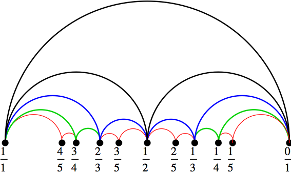
Figure 1. The Farey sequence of order $5$ and the triangulated hendecagon.

The main properties of Farey sequences can be found in [15]. A simple but important property is that every Farey sequence forms a triangulated polygon in the Farey graph. A Conway-Coxeter quiddity is then precisely the index of a Farey sequence, defined in [14].

The Conway-Coxeter theorem implies the following.

Corollary 8.7.

A solution $(a_{1},\ldots,a_{n})$ of Problem II is totally positive if and only if

$$a_{1}+a_{2}+\cdots+a_{n}=3n-6.$$

Indeed, the total number of triangles in a triangulation is $n-2$, and each triangle has three angles that contribute to a quiddity.

Remark 8.8.

The above formula is equivalent to Theorem 1 of [14]. Moreover, it holds not only for the complete Farey sequence, but also for an arbitrary path in the Farey graph. Consider the Farey sequence of order $5$ presented in Figure 1. It has many different shorter paths, for instance, $\left\{\frac{1}{1},\frac{2}{3},\frac{3}{5},\frac{1}{2},\frac{1}{3},\frac{0}{1}\right\}$.

8.5. Totally positive solutions of Problem III

A solution $(a_{1},\ldots,a_{n})$ of Problem III is totally positive if its double $(a_{1},\ldots,a_{n},a_{1},\ldots,a_{n})$ is a totally positive solution of Problem II. Every totally positive solution can be obtained from one of the solutions $(a_{1},a_{2})=(1,2)$, or $(2,1)$ by a sequence of operations (1.2).

The Conway-Coxeter theorem implies that there is a one-to-one correspondence between totally positive solutions of Problem III and centrally symmetric triangulations of $2n$-gons; see also [6].

Example 8.9.

There exist $70$ different centrally symmetric triangulations of the decagon, for instance

            

The corresponding sequences $(a_{1},a_{2},a_{3},a_{4},a_{5})=(5,2,2,2,1),\,(4,3,1,3,1),\,(4,2,1,4,1),\ldots$ are totally positive solutions of Problem III.

The total number of totally positive solutions of Problem III is given by the central binomial coefficient $\binom{2n}{n}=1,2,6,20,70,252,924,\ldots$

Acknowledgements. I am grateful to Charles Conley, Vladimir Fock, Alexey Klimenko, Ian Marshall, Sophie Morier-Genoud and Sergei Tabachnikov for multiple stimulating and enlightening discussions. I am also grateful to the referees for a number of useful comments and suggestions.

References

- [1] M. Aigner, Markov’s theorem and 100 years of the uniqueness conjecture. A mathematical journey from irrational numbers to perfect matchings. Springer, Cham, 2013.
- [2] K. Baur, R. Marsh, Frieze patterns for punctured discs, J. Algebraic Combin. 30 (2009), 349–379.
- [3] K. Baur, M. Parsons, M. Tschabold, Infinite friezes, European J. Combin. 54 (2016), 220–237.
- [4] F. Bergeron, C. Reutenauer, -tilings of the plane, Illinois J. Math. 54 (2010), 263–300.
- [5] C. Bessenrodt, T. Holm, P. Jorgensen, Generalized frieze pattern determinants and higher angulations of polygons, J. Combin. Theory Ser. A 123 (2014) 30–42.
- [6] C. Conley, V. Ovsienko Rotundus: triangulations, Chebyshev polynomials, and Pfaffians, to appear in Math. Intelligencer, arXiv:1707.09106.
- [7] J. H. Conway, H. S. M. Coxeter, Triangulated polygons and frieze patterns, Math. Gaz. 57 (1973), 87–94 and 175–183.
- [8] H. S. M. Coxeter. Frieze patterns, Acta Arith. 18 (1971), 297–310.
- [9] H. S. M.Coxeter, J. F. Rigby, Frieze patterns, triangulated polygons and dichromatic symmetry, The Lighter Side of Mathematics, R.K. Guy and E.Woodrow Eds., MAA Spectrum. Mathematical Association of America, Washington, DC, 1994, 15–27.
- [10] M. Cuntz, On Wild Frieze Patterns, Exp. Math. 26 (2017), 342–348.
- [11] M. Cuntz, I. Heckenberger, I Weyl groupoids of rank two and continued fractions, Algebra Number Theory 3 (2009), 317–340.
- [12] F. Delyon and B. Souillard, The rotation number for finite difference operators and its properties, Comm. Math. Phys. 89 (1983), 415–426.
- [13] P. Flajolet, M. Noy, Analytic combinatorics of non-crossing configurations, Discrete Math. 204 (1999), 203–229.
- [14] R. Hall, P. Shiu, The index of a Farey sequence, Michigan Math. J. 51 (2003), 209–223.
- [15] G. H. Hardy, E. M. Wright, An introduction to the theory of numbers. Sixth edition. Revised by D. R. Heath-Brown and J. H. Silverman. With a foreword by Andrew Wiles. Oxford University Press, Oxford, 2008, 621 pp.
- [16] C.-S. Henry, Coxeter friezes and triangulations of polygons, Amer. Math. Monthly 120 (2013), 553–558.
- [17] T. Holm, P. Jorgensen, A -angulated generalisation of Conway and Coxeter’s theorem on frieze patterns, arXiv:1709.09861.
- [18] I. Krichever, Commuting difference operators and the combinatorial Gale transform, Funct. Anal. Appl. 49 (2015), 175–188.
- [19] S. Morier-Genoud, Coxeter’s frieze patterns at the crossroads of algebra, geometry and combinatorics, Bull. Lond. Math. Soc. 47 (2015), 895–938.
- [20] S. Morier-Genoud, V. Ovsienko, R. Schwartz, S. Tabachnikov, Linear difference equations, frieze patterns and combinatorial Gale transform, Forum Math., Sigma, Vol. 2 (2014), e22 (45 pages).
- [21] S. Morier-Genoud, V. Ovsienko, S. Tabachnikov, -frieze patterns and the cluster structure of the space of polygons, Ann. Inst. Fourier, 62 (2012), 937–987.
- [22] S. Morier-Genoud, V. Ovsienko, S. Tabachnikov, -tilings of the torus, Coxeter-Conway friezes and Farey triangulations, Enseign. Math. 61 (2015), 71–92.
- [23] B. Simon, Sturm oscillation and comparison theorems, Sturm-Liouville theory, 29–43, Birkhäuser, Basel, 2005.
- [24] E. K. Sklyanin, The quantum Toda chain. Nonlinear equations in classical and quantum field theory, Lecture Notes in Phys., 226, Springer, Berlin, 1985, 196–233, .
- [25] D. Zagier, Nombres de classes et fractions continues, Journées Arithmétiques de Bordeaux (Conference, Univ. Bordeaux, 1974), Astérisque 24-25 (1975), 81–97.