Gas mass tracers in protoplanetary disks: CO is still the best

Abstract

Protoplanetary disk mass is a key parameter controlling the process of planetary system formation. CO molecular emission is often used as a tracer of gas mass in the disk. In this study we consider the ability of CO to trace the gas mass over a wide range of disk structural parameters and search for chemical species that could possibly be used as alternative mass tracers to CO. Specifically, we apply detailed astrochemical modeling to a large set of models of protoplanetary disks around low-mass stars, to select molecules with abundances correlated with the disk mass and being relatively insensitive to other disk properties. We do not consider sophisticated dust evolution models, restricting ourselves with the standard astrochemical assumption of $0.1~{}\mu$m dust. We find that CO is indeed the best molecular tracer for total gas mass, despite the fact that it is not the main carbon carrier, provided reasonable assumptions about CO abundance in the disk are used. Typically, chemical reprocessing lowers the abundance of CO by a factor of 3, compared to the case of photo-dissociation and freeze-out as the only ways of CO depletion. On average only 13% C-atoms reside in gas-phase CO, albeit with variations from 2 to 30%. CO₂, H₂O and H₂CO can potentially serve as alternative mass tracers, the latter two being only applicable if disk structural parameters are known.

1 Introduction

A young Sun-like star at its early evolutionary stage is generally surrounded by a flattened rotating gas and dust structure, which is commonly referred to as a protoplanetary disk even though evidence of planet formation in these disks is still mostly circumstantial (see, e.g., reviews by Williams & Cieza, 2011; Armitage, 2015). While the exact scenario of planet formation remains debated, the mass of the protoplanetary disk is thought to play a key role in this process (Mordasini et al., 2012; Bitsch et al., 2015). Therefore, estimating accurate disk masses from observations is one of the most important but also most challenging tasks in studies of formation and early evolution of planetary systems.

There are two different approaches to measuring disk masses. The most common way is to observe the dust continuum emission. Provided this emission is optically thin (which is expected at sub-millimeter and millimeter wavelengths), one can calculate the total dust mass in the disk (Andrews & Williams, 2005; Williams & Cieza, 2011) from the integrated continuum flux. Then, to convert the dust mass into a total disk mass, standard interstellar gas-to-dust ratio of 100 can be adopted (Bohlin et al., 1978). However, to apply this method one needs to know the dust temperature in the disk, because the same flux at a given wavelength may come both from larger amount of cold dust or from a smaller amount of warm dust. Such a mass derivation requires assumptions about dust optical properties, which are not well constrained for dust grains in protoplanetary disks and also may change as dust grows at early stages of planet formation (Draine, 2006; Henning & Meeus, 2011). Furthermore, it is far from obvious that interstellar gas-to-dust mass ratio is valid for protoplanetary disks. Dunham et al. (2014) and Tsukamoto et al. (2017) suggest that masses of young disks derived from dust observations may be underestimated.

The more direct way to measure gas mass in disks is to observe molecular emission lines. While disks mostly consist of molecular hydrogen and helium, these components either cannot be observed directly, or trace only a limited disk region (see e.g. Carmona et al., 2011), and other mass tracers are commonly employed, which require knowledge of a conversion factor from tracer mass to H₂ mass. In this respect, hydrogen deuteride (HD) seems to be a good candidate (Bergin et al., 2013; McClure et al., 2016), as it is well coupled to molecular hydrogen and also has a relatively high abundance of $3\cdot 10^{-5}$ relative to H₂, although using it as a mass tracer may lead to a factor of  3 uncertainty (Trapman et al., 2017). Currently, the only facility to produce new HD measurements will be SOFIA with its forthcoming HIRMES spectrograph.

A widely used molecular mass tracer in disks is carbon monoxide (CO), as it is one of the most abundant species in the interstellar and circumstellar material and possesses rotational transitions that are easy to observe. The hydrogen mass determination using CO lines is usually applied to diffuse clouds (Goldsmith et al., 1997; Bolatto et al., 2013), but now it is also commonly used for protoplanetary disks (Williams & Best, 2014; Ansdell et al., 2016; Williams & McPartland, 2016; Miotello et al., 2016). But the CO-based disk mass determination method has some recognized problems, too. First, CO emission is optically thick, which can be circumvented by observing CO isotopologues ¹³CO, C¹⁸O, and C¹⁷O, and also ¹³C¹⁸O, which has been recently observed in the TW Hya disk (Zhang et al., 2017). Their lines are typically optically thin as they are less abundant (Qi et al., 2011). The second problem is that CO along with its isotopologues freezes out in cold dense regions of the disk midplane and gets non-observable (Henning & Semenov, 2013).

Given the lack of good alternatives, CO observations are still vital for the determination of protoplanetary disk mass. However, its application for that purpose should be validated with theoretical models comprising both radiation transfer and chemistry. Williams & Best (2014) constructed a model of CO distribution over a selection of parameterized protoplanetary disks, assuming that CO is frozen in those regions of the disk where the temperature is below 20 K and is photo-dissociated above the vertical H₂ column density of $1.3\times 10^{21}$ cm^-2. In the remaining part of the disk the CO abundance relative to H₂ was assumed to be equal to the so-called ‘interstellar’ value, $10^{-4}$ (France et al., 2014). Williams & Best (2014) pointed out that under these assumptions, CO mass in this warm molecular zone represents a significant fraction of the total CO mass and thus traces the bulk of the disk gas mass. However, the CO-based disk gas masses derived so far seem to be systematically smaller than masses derived from dust observations. ALMA disk surveys in Lupus, Chamaeleon, $\sigma$ Orionis and other star-forming regions by Ansdell et al. (2016, 2017) based on the same theoretical model suggest very high dust-to-gas mass ratios up to $1/10$.

Williams & Best (2014) suggested that the difference between the CO-based disk mass and the dust-based disk mass can be both real (reflecting low gas-to-dust mass ratios) and related to an uncertainty in the CO-to-H₂ abundance ratio, if, for example, some other CO depletion pathways are more efficient. This possibility was explored by Miotello et al. (2016) with the isotope-selective chemical model by means of artificially reduced carbon abundance. However, they only considered simple hydrogenation surface processes, which may somewhat decrease gas-phase CO abundance. They noted that the uncertainty in the CO-based gas mass estimate can be reduced if some information on the disk structure is available. A continuation of this study was presented by Miotello et al. (2017), who confirmed that simplified surface chemistry may be the cause of discrepancy of disk masses estimated using CO and dust observations.

A more detailed surface chemistry model was utilized in the work of Yu et al. (2016). These authors considered CO evolution in the model of an accretion-heated disk and found that even inside a CO snowline a gas-phase CO abundance can be reduced significantly due to conversion of CO into other less volatile species, like CO₂ and complex organic molecules (COMs), which is a common effect at various stages of star formation (Vasyunina et al., 2012). However, only a limited number of disk models was considered in this study, and only an inner part of the disk (within 70 au) was analyzed. Also, Yu et al. (2016) assumed that a significant dust evolution has already taken place in the disks, so that most dust grains have coagulated into larger particles, limiting efficiency of both CO freeze-out and surface conversion into other molecules. Yu et al. (2017) extended this study and came to the conclusion that the chemical depletion of CO may lead to significant underestimation of the disk gas masses.

In this study we intend to combine a large grid of disk physical models with a comprehensive chemical model, which includes detailed treatment of surface chemistry. We check the degree of reliability of CO as a gas mass tracer with realistic variations of disk parameters and the uncertainties related to CO chemical depletion. We perform an analysis of the carbon partition into the gas and solid species. The computed set of models is used to look for other possible tracers of disk gas mass.

2 Model

The basis for our study is a set of $\sim 1000$ disk models (described in detail in Section 2.3), which allows studying the distribution of gas-phase and surface molecular abundances for a selection of disk structural parameters. We utilize a modified version of the ANDES code (Akimkin et al., 2013) combined with the updated ALCHEMIC network (Semenov & Wiebe, 2011) to follow the evolution of molecular abundances.

2.1 Physical Structure

For the parameterization of the disk surface density we adopt the commonly used tapered power-law profile (Hartmann et al., 1998)

$$\Sigma\left(R\right)=\Sigma_{0}\left(\frac{R}{R_{\rm c}}\right)^{-\gamma}e^{-\left(R/R_{\rm c}\right)^{2-\gamma}},$$ (1)

where $\Sigma_{0}$, g cm^-2, is the surface density normalization, $\gamma$ parameterizes the radial dependence of the disk viscosity, $R_{\rm c}$ is a characteristic radius of the disk. $\Sigma_{0}$ can be calculated from the total disk mass as

$$\Sigma_{0}=\frac{M_{\rm disk}\left(2-\gamma\right)}{2\pi R_{\rm c}^{2}}.$$ (2)

So, the surface density radial profile depends on three parameters: $M_{\rm disk}$, $\gamma$, $R_{\rm c}$.

We assume that the disk is axially-symmetric and its vertical structure at each radius is determined by the hydrostatic equilibrium

$$\frac{\partial P\left(R,z\right)}{\partial z} = -\rho\left(R,z\right)\frac{zGM_{\star}}{\left(R^{2}+z^{2}\right)^{3/2}},$$ (3)

$$P = \frac{k_{\rm B}T\left(R,z\right)}{\mu m_{\rm p}}\rho\left(R,z\right),$$ (4)

where the disk temperature distribution $T\left(R,z\right)$ is calculated using a simple parameterization (Williams & Best, 2014; Isella et al., 2016)

$$T\left(R,z\right)=\begin{cases}T_{\rm a}(R,z=z_{\rm q})+\left[T_{\rm m}(R)-T_{\rm a}(R,z=z_{\rm q})\right]\left(\cos\frac{\pi z}{2z_{\rm q}(R)}\right)^{2},&\text{if $\left|z\right|<z_{\rm q}(R)$},\\ T_{\rm a}(R,z),&\text{if $\left|z\right|\geqslant z_{\rm q}(R)$}.\end{cases}$$ (5)

Rather than adding disk atmosphere and midplane temperatures $T_{\rm m}$ and $T_{\rm a}$ to our set of parameters, we calculate them on the base of central luminosity source (star plus accretion region). The optically thin disk atmosphere can be easily ray-traced as dust thermal radiation does not contribute significantly into the source function. The dust temperature is determined from the thermal balance equation:

$$\int\limits_{0}^{\infty}\kappa_{\nu}J_{\nu}d\nu=\int\limits_{0}^{\infty}\kappa_{\nu}B_{\nu}(T_{\rm a})d\nu$$ (6)

where $\kappa_{\nu}$, cm^-1 is the dust absorption coefficient and $J_{\nu}$ is the mean intensity of radiation coming directly from the central star, accretion region and interstellar medium,

$$J_{\nu}=J_{\nu,\rm s}+J_{\nu,\rm acc}+J_{\nu,\rm ISRF}=W_{\star}B_{\nu}(T_{\star})e^{-\tau_{\nu,1}}+W_{\rm acc}B_{\nu}(T_{\rm acc})e^{-\tau_{\nu,1}}+\frac{1}{3}I_{\rm ISRF}(e^{-\tau_{\nu,2}}+e^{-\tau_{\nu,3}}+e^{-\tau_{\nu,4}}).$$ (7)

Here $W_{\star}=\frac{1}{4}R_{\star}^{2}/(R^{2}+z^{2})$ and $W_{\rm acc}=\frac{1}{4}R_{\rm acc}^{2}/(R^{2}+z^{2})$ represent the dilution factors for the radiation from the central star and accretion region, $R_{\star}$ and $T_{\star}$ are stellar radius and effective temperature. Accretion luminosity is simulated by the additional central source of irradiation with effective radius $R_{\rm acc}$ and effective temperature $T_{\rm acc}$, so that $L_{\rm acc}=4\pi R_{\rm acc}^{2}\sigma_{\rm SB}T_{\rm acc}^{4}=(3/2)\,GM_{\star}\dot{M}/R_{\star}$. We assume a typical accretion rate of $\dot{M}=10^{-8}M_{\odot}$ yr^-1 and $T_{\rm acc}=15\,000$ K to calculate the effective radius of an accretion region, $R_{\rm acc}$. The interstellar radiation field is adopted from Mathis et al. (1983).

The optical depth in (7), $\tau_{\nu,k}=\int(\kappa_{\nu}+\sigma_{\nu})dl$, is calculated along four directions: to and from the star ($k=1,2$), and up and down ($k=3,4$). Dust optical properties are computed from the Mie theory for astrosilicate grains (Laor & Draine, 1993) assuming dust-to-gas ratio of 0.01. We use a spatial grid $R_{n}$ and $z_{nm}$ such that $z_{nm}/R_{n}$ is constant for a given $m$. This greatly reduces the computational cost for the ray-tracing procedure as all spatial points with fixed $m$-index are located on the same line.

We define $z_{\rm q}(R)$ as the height at which $T_{\rm a}$ has a maximum at a given $R$. Above $z_{\rm q}(R)$ dust temperature decreases with $z$ due to increasing distance from the star, the drop of temperature below $z_{\rm q}(R)$ is explained by the absorption. This also means that the source function starts to be dominated by the dust thermal infrared radiation and not by the radiation from star. In this regime the approximation for radiation intensity (7) is no longer valid. The temperature profile below $z_{\rm q}(R)$ is set according to (5) with the midplane temperature adopted from the optically thick case of the two-layered model (Chiang & Goldreich, 1997; Dullemond et al., 2001)

$$T_{\rm m}^{4}(R)=\frac{1}{2}\varphi\left[T_{\star}^{4}\left(\frac{R_{\star}}{R}\right)^{2}+T_{\rm acc}^{4}\left(\frac{R_{\rm acc}}{R}\right)^{2}\right],$$ (8)

where $\varphi=0.05$ is a flaring angle (Dullemond & Dominik, 2004), the factor $\frac{1}{2}$ reflect the fact that only half of the infrared radiation from the disk super-heated upper layer heats the midplane, and the other half is emitted outward. This midplane temperature differs from the disk effective temperature by a factor of $\sqrt[4]{2}$. Gas and dust temperatures are assumed to be equal. We use iterations to obtain self-consistent density and temperature structures, which is important for the ray-tracing procedure and calculation of the atmosphere temperature. However, in the calculation of the midplane temperature we keep the flaring angle fixed to avoid disk self-shadowing as this effect must be studied by means of a more sophisticated model. The adopted model for the disk physical structure enables us to perform astrochemical simulations for a large set of models while keeping the adequate level of accuracy.

Values of the stellar radius $R_{\star}$, effective temperature $T_{\star}$ and stellar mass $M_{\star}$, used in the above parameterizations, are not independent. We take $M_{\star}$ as a primary parameter and calculate $R_{\star}$ and $T_{\star}$ from evolutionary tracks by Baraffe et al. (2015), assuming a stellar age of 3 Myr. As their model is restricted to low-mass stars, we consider only T Tauri-type stars with masses between 0.5 and 1.4 $M_{\sun}$. Stellar and accretion luminosities are assumed to be constant during the chemical run. However, luminosity bursts may have a lasting impact on the disk chemical structure and are a topic of current research (Harsono et al., 2015; Rab et al., 2017).

Overall, we have four parameters, $M_{\rm disk}$, $\gamma$, $R_{c}$, and $M_{\star}$, which determine the physical structure of the disk. The spatial grid has 50 points in radial direction between 1 and 1000 au and 80 points in vertical direction from the midplane to $z/R=0.5$.

2.2 Chemical Model

The chemical structure is calculated with the modified version of the thermochemical non-equilibrium ANDES code (Akimkin et al., 2013). The system of chemical kinetics equations was updated to account for the gas-grain chemistry of the ALCHEMIC model (Semenov & Wiebe, 2011). The gas-phase part was benchmarked with the NAHOON code (Wakelam et al., 2015), which resulted in fixing several non-critical bugs. Some rate coefficients were updated in accordance with the KIDA14 database. Overall, the chemical network contains 650 species involved in 7807 reactions. No isotope-selective chemistry is considered.

The original version of the ANDES code contains a module to calculate thermal balance of gas and dust. We replaced this module in the current study by a phenomenological setup for the thermal structure in order to reduce computational costs for modeling a large set of disks. However, the 2D radiation transfer (RT) of UV radiation was implemented in order to calculate photoreaction rates. The RT is based on the short characteristics method and allows for the radiation field calculation up to optical depths $\tau_{\rm UV}\sim 10$. The MRN grain size distribution (Mathis et al., 1977) and dust-to-gas ratio of 0.01 are taken as the dust model for the RT modeling in the disk atmosphere. We calculate radiation transfer for the stellar and interstellar radiation field and also consider X-rays, cosmic rays (CR), and radioactive nuclides as sources of ionization. The spectrum of a central star is assumed to be a black body with an effective temperature corresponding to a given stellar mass plus an UV excess produced by accretion (as stated above). While the real stellar spectra may not be well represented by black body, in the context of our study only the relation between the visible and far-UV spectrum parts is important. The X-ray ionization rate is calculated on the base of Bai & Goodman (2009) model (their eq. [21]), assuming X-ray luminosity $L_{\rm X}=10^{30}$ erg s^-1 and $T_{\rm X}=3$ keV. We use $\zeta_{0}=1.3\times 10^{-17}$ s^-1 for unattenuated CR ionization rate and attenuation length of 96 g cm^-2 (Sano et al., 2000) and $\zeta_{\rm RA}=6.5\times 10^{-19}$ s^-1 for ionization rate by radioactive elements.

The initial abundances are presented in Table 1 and correspond to the ‘low-metals’ case of Lee et al. (1998), unless otherwise noted.

Table 1: Initial abundances (relative to H-nuclei).

Species	H2	H	He	C+	N	O	S+
Abundance	0.499	0.002	0.09	$7.3\cdot 10^{-5}$	$2.14\cdot 10^{-5}$	$1.76\cdot 10^{-4}$	$8\cdot 10^{-8}$
Species	Si+	Fe+	Na+	Mg+	P+	Cl+
Abundance	$8\cdot 10^{-9}$	$3\cdot 10^{-9}$	$2\cdot 10^{-9}$	$7\cdot 10^{-9}$	$2\cdot 10^{-10}$	$1\cdot 10^{-9}$

Apart from gas-phase processes, our chemical network includes surface reactions along with accretion and desorption. As many species tend to freeze out onto dust particles, which makes them unobservable, surface chemistry is crucial for such models. We adopt the ratio of diffusion energy to desorption energy of 0.5 and account for tunneling through reaction barriers. Single-layer surface chemistry is considered. Our treatment of surface chemistry includes reactive desorption with the efficiency of $1\%$, which means that in two-body surface reactions 99$\%$ of product species stay on the surface and 1$\%$ are released into gas, although more detailed treatment of reactive desorption is already available in some astrochemical models (Vasyunin et al., 2017). The representative size of dust grains in grain chemistry treatment is assumed to be $0.1\mu$m. In protoplanetary disks dust is supposed to grow, which reduces the available dust surface and slows down the surface chemistry. Also grown dust makes disk more transparent to stellar radiation. However, the theoretical description of dust evolution is a complicated task, especially taking into account such poorly studied effects as grain charging (Okuzumi, 2009; Akimkin, 2015; Ivlev et al., 2016). Therefore we neglect dust evolution effects and focus on varying disk macrophysical parameters.

2.3 Set of Models

Like Williams & Best (2014), we create a grid of models with variable parameters responsible for the disk physical structure. As we have already mentioned, these parameters are disk mass $M_{\rm disk}$, stellar mass $M_{\star}$, effective radius of the disk $R_{\rm c}$, and power-law index $\gamma$. We vary them within bounds typical for protoplanetary disks around T Tauri stars. Specific ranges for each parameter are presented in Table 2.

Table 2: Range of parameters used in the set of models.

Parameter	Value
$M_{\rm disk}$	$10^{-4}\div 10^{-1}M_{\odot}$
$M_{\star}$	$0.5\div 1.4M_{\odot}$
$R_{\rm c}$	$30\div 200$ au
$\gamma$	$0.5\div 1.5$

We calculate 2D distributions of 650 species for time moments of 0.5, 1, and 3 Myr and use these distributions to compute total species masses in the disk. In Section 3.1 we employ a random set of models, with every parameter being uniformly distributed inside the ranges (for disk mass it is $\log_{10}M_{\rm disk}$ that is distributed uniformly). In Section 3.3 we use a grid of models with fixed nodes and present various cuts through the parameter space.

3 Results

3.1 Potential gas mass tracers

The list of molecules observed in protoplanetary disks is currently not very extensive, including CN, HCN, HNC, CS, SO, H₂CO, CCH, HC₃N, CH₃CN, C₃H₂, C₂H₂, OH, HCO⁺, N₂H⁺, CH⁺, C⁺, O, NH₃, CH₃OH (Dutrey et al., 1997; Thi et al., 2011; Dutrey et al., 2011; Chapillon et al., 2012; Qi et al., 2013; Öberg et al., 2015; Walsh et al., 2016; Guilloteau et al., 2016; Salinas et al., 2016). It would be interesting to find out if some of them could possibly serve as a gas mass tracer alternative to commonly used CO. Also, pending future discoveries of molecules in protoplanetary disks, we do not exclude from consideration other chemical species present in the model.

The total disk abundance of a prospective disk mass tracer $X_{i}=N_{i}/N_{\rm<H>}$ should be correlated with the disk mass, while being less dependent on other physical properties of the disk, such as the density profile, disk radius or properties of the central star. The correlation should not necessarily be linear, implying independence of the total abundance on the disk mass. In principle, the species abundance can be any monotonic function of the disk mass. Also, it should not vary significantly with time.

To assess the species potential applicability as a disk mass tracer, we need to introduce some quantitative gauges. For every $j$th disk model in the ensemble we calculate the total logarithmic abundance of $i$th species $x_{ij}=\log_{10}\left(X_{ij}\right)$. The value $\overline{x_{i}}$, averaged over the disk model ensemble, represents a typical (logarithm of) total disk abundance of an $i$th species. We employ its dispersion $s^{2}_{i}=\overline{(x_{ij}-\overline{x_{i}})^{2}}$ as a simple quantitative measure of suitability of $i$th species as a mass tracer. Further we refer to the standard deviation $s$ as a ‘scatter parameter’ to stress the limitation of the approach. First, the distribution of protoplanetary disks parameters is not well known and quite probably differs from the uniform distribution assumed during the disk ensemble generation. Second, the scatter may not reflect the non-linear scaling between disk and species mass. However, generally speaking, the smaller is the scatter, the better the species performs as a mass tracer.

Table 3 summarizes this simple statistical analysis and contains total disk abundances and scatter parameters for the model age of 3 Myr, sorted by increasing $s_{i}$. For other chemical ages the values of scatter parameter are about the same, slightly growing with time. We include components with average total disk abundance greater than $10^{-11}$, excluding ices and common species like H₂ and He. All the detected species listed above are present in the table as well. The species that are potentially observable with JWST but not with ALMA are marked with a star (^⋆). Total disk abundances for ice species are given in the appendix in the table, analogous to Table 3.

Table 3: Average total disk abundance $\overline{X_{i}}=10^{\overline{x_{i}}}$ and scatter $s_{i}$ for selected species.

Species	$\overline{X_{i}}$	$s_{i}$, dex	Species	$\overline{X_{i}}$	$s_{i}$, dex	Species	$\overline{X_{i}}$	$s_{i}$, dex
N2	$2.0\times 10^{-6}$	0.25	C6	$1.5\times 10^{-11}$	0.45	C	$4.9\times 10^{-6}$	0.64
NH3	$3.2\times 10^{-9}$	0.27	HCN	$2.4\times 10^{-9}$	0.45	O3	$5.5\times 10^{-8}$	0.64
CH3	$3.6\times 10^{-10}$	0.28	Si	$1.7\times 10^{-10}$	0.46	O	$2.1\times 10^{-5}$	0.66
CO	$8.0\times 10^{-6}$	0.28	C4H	$10.0\times 10^{-11}$	0.46	C2H6	$2.3\times 10^{-9}$	0.66
H${}_{3}^{+}$	$2.2\times 10^{-10}$	0.28	⋆C2H2	$4.3\times 10^{-10}$	0.47	CH${}_{3}^{+}$	$3.8\times 10^{-11}$	0.73
⋆CO2	$5.2\times 10^{-7}$	0.28	Na	$1.9\times 10^{-10}$	0.48	C2H	$6.6\times 10^{-10}$	0.74
H2CO	$1.3\times 10^{-10}$	0.29	N2H+	$1.3\times 10^{-11}$	0.48	Na+	$1.8\times 10^{-10}$	0.74
H3O+	$2.6\times 10^{-10}$	0.30	CS	$4.7\times 10^{-10}$	0.49	N	$1.5\times 10^{-6}$	0.75
H2CN+	$1.6\times 10^{-11}$	0.31	Mg	$4.0\times 10^{-11}$	0.49	H5C3N	$2.2\times 10^{-11}$	0.77
H2CS	$1.6\times 10^{-11}$	0.32	H2C3O	$4.7\times 10^{-10}$	0.50	CH2	$5.6\times 10^{-10}$	0.77
NH2	$3.5\times 10^{-10}$	0.32	MgH2	$5.2\times 10^{-10}$	0.50	HC2O	$6.9\times 10^{-11}$	0.80
SO2	$2.1\times 10^{-10}$	0.32	HS	$2.1\times 10^{-10}$	0.51	N2O	$1.2\times 10^{-10}$	0.81
HNO	$1.4\times 10^{-10}$	0.33	CH2CO	$1.8\times 10^{-10}$	0.51	S+	$4.9\times 10^{-9}$	0.81
C3	$1.3\times 10^{-8}$	0.34	CH5N	$2.5\times 10^{-11}$	0.51	HCCN	$5.0\times 10^{-11}$	0.81
C5H3	$2.5\times 10^{-11}$	0.35	⋆H2O	$4.0\times 10^{-7}$	0.51	P+	$1.1\times 10^{-11}$	0.82
SO	$2.7\times 10^{-9}$	0.37	Cl	$1.8\times 10^{-10}$	0.51	Si+	$5.1\times 10^{-10}$	0.83
C3H	$1.1\times 10^{-10}$	0.39	CH3CN	$2.0\times 10^{-11}$	0.52	CH	$1.5\times 10^{-9}$	0.83
OCN	$1.7\times 10^{-10}$	0.40	HNC	$1.2\times 10^{-9}$	0.52	Fe+	$1.6\times 10^{-10}$	0.84
⋆OH	$1.4\times 10^{-8}$	0.41	H2O2	$4.0\times 10^{-9}$	0.53	Mg+	$3.3\times 10^{-10}$	0.84
P	$1.5\times 10^{-11}$	0.41	C4H2	$2.4\times 10^{-11}$	0.53	O2H	$1.3\times 10^{-11}$	0.85
HC3O	$3.2\times 10^{-11}$	0.41	C2H4	$1.7\times 10^{-11}$	0.54	CN	$1.4\times 10^{-9}$	0.86
H2S	$1.3\times 10^{-9}$	0.41	C5	$1.1\times 10^{-10}$	0.54	HC3N	$1.6\times 10^{-11}$	0.86
FeH	$2.4\times 10^{-10}$	0.42	C3H2	$8.7\times 10^{-11}$	0.54	C+	$1.5\times 10^{-6}$	0.88
C4	$1.6\times 10^{-10}$	0.43	C5H2	$2.1\times 10^{-11}$	0.55	C9H2	$2.3\times 10^{-11}$	0.94
NO	$4.1\times 10^{-9}$	0.43	⋆CH4	$7.7\times 10^{-8}$	0.55	C5H4	$2.9\times 10^{-11}$	0.97
NH	$9.6\times 10^{-11}$	0.43	CH3OH	$9.3\times 10^{-11}$	0.56	C2	$1.2\times 10^{-9}$	1.02
S	$6.5\times 10^{-9}$	0.43	C5H	$2.2\times 10^{-11}$	0.57	CH2NH2	$4.8\times 10^{-11}$	1.09
SiO	$3.4\times 10^{-10}$	0.43	CH2OH	$4.1\times 10^{-11}$	0.59	CH3NH	$4.7\times 10^{-11}$	1.09
⋆O2	$2.4\times 10^{-6}$	0.44	HCO+	$8.7\times 10^{-11}$	0.60	CH+	$3.7\times 10^{-13}$	1.19
HNCO	$1.9\times 10^{-9}$	0.44	HCOOH	$1.3\times 10^{-11}$	0.63	N2H2	$6.9\times 10^{-11}$	1.22

The top of the table is occupied by N₂, NH₃, CH₃, CO, H${}_{3}^{+}$, and CO₂, and in Fig. 1 their total masses are shown as functions of the total disk mass. In each panel a solid line is shown with the slope corresponding to linear scaling of the species mass with the disk mass at the average total abundance $\overline{X_{i}}=10^{\overline{x_{i}}}$ from Table 3. A scatter parameter is also indicated in each panel. Molecular nitrogen seem to be the best theoretical mass tracer as its mass scales almost linearly with the disk mass over the entire range of considered disk masses. This molecule, like H₂, has no rotational transitions and thus cannot be observed directly, but ¹⁴N¹⁵N has. Despite the mass difference between ¹⁴N and ¹⁵N is small and hence the dipole moment is very weak, theoretically, one could detect its fundamental rotational line at 4.34 $\mu$m in disks.

The CO total mass also shows nearly linear scaling with the disk mass, but with a scatter that increases somewhat in more massive disks. Disks with lower $\gamma$ values (shallower density profiles) tend to have smaller CO abundance, while more compact disks (with lower $\gamma$ and $R_{\rm c}$, i.e. smaller and redder dots in Fig. 1) are more CO rich. The reason is that in a compact disk most mass is located in a warm disk area, where CO freeze-out is prohibited. As we consider larger and/or shallower disks, more mass is shifted to colder disk areas.

The dashed line in the top left panel of Fig. 1 indicates the maximum possible CO mass, corresponding to the assumption that all carbon atoms are locked in gas-phase CO. In this extreme case $M_{\rm CO}=1.5\times 10^{-3}M_{\rm disk}$. According to our results, the computed total CO mass is much lower in all the considered models, and its typical value is only $1.7\times 10^{-4}M_{\rm disk}$. Most carbon atoms are locked up not in CO but in CO₂ ice. Carbon redistribution is discussed in more detail in Section 3.2.

The scatter parameter for NH₃ and CH₃ is formally somewhat lower than the one for CO. However, inspection of Fig. 1 shows that masses of these species depend stronger on the disk structure, than the CO mass, if the disk mass exceeds $\sim 10^{-3}\,M_{\odot}$. Also, ammonia masses loose linear scaling with disk masses in the least massive disks. Additionally, abundances of NH₃ and CH₃, as well as the one of H${}_{3}^{+}$, are quite low, which hampers their detection. While NH₃ has nevertheless been detected by Herschel in nearby TW Hya disk (Salinas et al., 2016), methyl radical and H${}_{3}^{+}$ have no allowed dipole moment as they are symmetric and planar. Potentially H${}_{3}^{+}$ can be traced by o-H₂D⁺, thus, even though we do not consider isotopic chemistry, o-H₂D⁺ may also correlate well with the disk gas mass. However, detecting this species in disks is challenging even for ALMA (Chapillon et al., 2011).

Carbon dioxide looks quite promising. Its scatter only slightly exceeds that of CO and it will also be observable by JWST. While the dependence of its mass on the disk mass is non-linear in disks with the lowest masses, but this is compensated by uniformly low scatter and linear scaling for disks with masses above $\sim 10^{-3}\,M_{\odot}$.

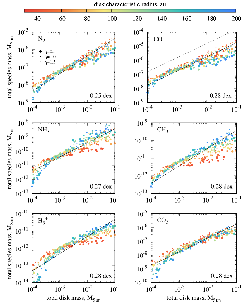
Figure 1: Total mass of species with lowest scatter values in the disk as a function of the disk mass at an age of 3 Myr. Point size depicts $\gamma$-value (larger symbols represent shallower surface density profiles), point color represents disk characteristic radius $R_{\rm c}$. Solid lines indicate linear scaling with the slope equal to average mass fraction. Dashed line corresponds to CO amount if it would contain all the available carbon atoms. The scatter parameter is shown in the right bottom corner of each panel.

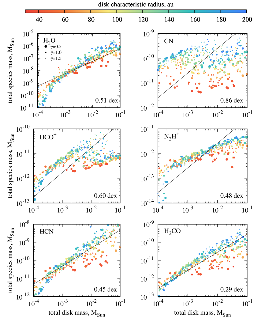
Figure 2: Same as in Fig. 1, but for species with higher scatter values.

Overall, we conclude that currently CO is the best mass tracer combining ease of detection and predictability of behavior. Among other species some are better than others, with the scatter comparable to the one of CO (see Fig. 2). Water mass scales with the disk mass for $M_{\rm disk}>10^{-3}\,M_{\odot}$, but in the least massive disks water abundance shows a significant scatter (of about two orders of magnitude), with smaller $\gamma$ values and more extended disks corresponding to lower water masses. This seems to be interesting in a view of diverse results of Herschel water observations in disks of DM Tau (Bergin et al., 2010) and TW Hya (Hogerheijde et al., 2011). Quite different water abundances may reflect not only evolutionary changes, but also structural variations.

Other carbon-bearing species show a significant scatter across the entire disk mass range, and the scatter generally increases as the disk mass increases. But in some cases the uncertainty can be reduced significantly if the disk size is known. Intriguingly, the H₂CO emission detected in disks could potentially be used as a proxy of disk mass, since the H₂CO-disk mass factor has a low scatter similarly to CO and is quite tight (albeit non-linear), if most compact disks are excluded. On the other hand the H₂CO emission in disks shows peculiar ring-like structure (Henning & Semenov, 2008; Loomis et al., 2015; Öberg et al., 2017), which makes such an analysis a difficult endeavor. The CN and HCO⁺ scaling is sufficiently non-linear that hampers their usage as mass tracers.

An interesting case is represented by N₂H⁺. Dependence of its mass on the disk mass is quite tight over the entire $M_{\rm disk}$ range and shows extreme sensitivity to the disk mass for $M_{\rm disk}<3\times 10^{-4}\,M_{\sun}$. However, at higher $M_{\rm disk}$ values the dependence of N₂H⁺ mass on the disk mass is much weaker. This should be related to the CO behavior. In extremely low-mass disks CO is depleted from the gas phase only due to freeze out. In more massive disks CO also experiences the chemical depletion due to carbon redistribution into other species. The steeper left part of the N₂H⁺ graph (see Fig. 2) reflects the developing chemical depletion of CO, while at the shallower right part this process is saturated. The change of N₂H⁺ abundance in more massive disks is explained by the shift of N₂H⁺ from the midplane to upper layers.

3.2 Carbon redistribution

In this section we consider major carbon-bearing species and demonstrate that gaseous CO is not the main reservoir of carbon in the considered protoplanetary disks. For each disk we find molecules which are major carbon reservoirs and calculate what percentage of carbon they comprise. The distribution of carbon among top-ten carbon-bearing species is plotted in Fig. 3. Three time moments are presented, 0.5, 1, and 3 Myr, showing that this distribution does not change much with the disk age.

There are two reasons for such a behavior. First, we show carbon fraction integrated over the entire disk, and most of material contributing to this value is relatively warm and dense, allowing chemical equilibrium to be reached within 0.5 Myr. Second, shown ice species are relatively simple, and their formation does not involve long-scale surface chemistry, so that they also have short typical chemical timescales.

We do see, however, some temporal changes in the carbon fraction for some species. The fraction of CO₂ ice gradually increases with time, while fractions of CO in gas and ice diminish mostly due to conversion of iCO into iCO₂ on the dust surfaces. Other molecules fractions also demonstrate some trends, so the redistribution of carbon in disks slowly continues during the considered time.

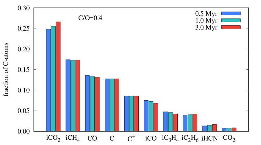
Figure 3: Distribution of carbon between major carbon-bearing molecules for different disk ages, averaged over the models. Ice species are denoted by leading ‘i’. C/O=0.4 is a ratio of carbon and oxygen elemental abundances.

The diagram in Fig. 3 shows that carbon is mostly locked in CO₂-ice (27$\pm$8%) at 3 Myr, but a sufficient fraction of carbon stays in elementary forms of C or C⁺. Among ten major carbon-bearing molecules, which constitute 95% of all available C atoms, only four are in the gas phase. The most abundant gas-phase species is CO with an average of 13%, while gas-phase CO₂ comprises only about 1%. In other words, only every seventh C atom belongs to CO in a gas form. The prevalence of the CO₂ ice, which is mostly formed on grains, stresses the necessity of proper surface chemistry treatment.

In Fig. 4 we present distribution over the disk of important C-containing molecules for a model with typical parameters ($M_{\rm disk}=0.01~{}M_{\sun}$, $M_{\star}=1.0~{}M_{\sun}$, $R_{\rm c}=100$ au, and $\gamma=0.8$). Despite CO snowline is expected to be located at $\sim 70$ au, where the temperature reaches the critical value of 20 K, we see lack of gaseous CO in the disk midplane as close to the star as $\sim$15 au. Even within the CO snowline in a region with temperature just above 20 K there is constant exchange of CO molecules between gas and ice reservoirs. Here some of temporally frozen-out CO molecules are apparently converted into CO₂ ice before they go back to the gas. Black and gray contours in Fig. 4 indicate the area, limited by the criteria outlined by Williams & Best (2014): CO is supposed to reside in the gas-phase everywhere except for the regions where it is frozen out ($T<20$ K) or photo-dissociated ($\Sigma_{\rm H_{2}}<1.3\times 10^{21}$ cm^-2). But in our model CO is not only highly depleted inside the restricted area due to chemical redistribution into other molecules, but it is also present outside of this area. Specifically, we see some CO in the outer disk region, which is shadowed from the star. In this cold region CO is photo-desorbed from dust grains, but not photo-dissociated by interstellar UV due to H₂ shielding. This allows CO to be present in the gas phase despite temperatures below the freezing point.

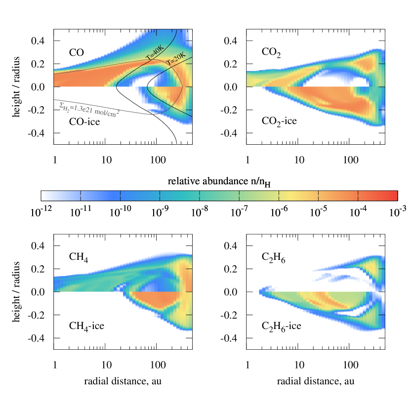
Figure 4: Abundances of major carbon-bearing species over the disk at the age of 3 Myr, for one particular model ($M_{\rm disk}=0.01~{}M_{\sun}$, $M_{\star}=1.0~{}M_{\sun}$, $R_{\rm c}=100$ au, and $\gamma=0.8$). Upper half of the plots corresponds to gas abundances, while the bottom half shows ice abundances.

In our set of models average total abundance ratio iCO₂/iH₂O is 1/3. For the model shown in Fig. 4 the iCO₂/iH₂O abundance ratio varies with radius from 10% to 110% in the 6–120 au range with maximum at 20 au. CO-ice dominates over CO₂-ice beyond 200 au with maximum abundance ratio relative to water of 60% at 300 au. These characteristic abundance ratios are consistent with what is observed in most comets (Mumma & Charnley, 2011). However, comparing our results to cometary abundances, one has to keep in mind that abundances of molecules observed in comets depend also on the nuclei structures and their thermal evolution (e.g. Hässig et al., 2015) and on the molecule processing in comae. The dynamical evolution of the comet ensemble is also of importance. In our model this ratio is computed for a large range of models and may differ from the corresponding ratios in specific models and/or spatial locations.

The CO₂ snowline is clearly seen at $\sim$6 au, and a significant amount of CO₂ ice resides in the disk dark regions up to distances of about 300 au from the star. Another abundant ice, methane, has a snowline at about 20–30 au from the star and is quite abundant in the midplane from 30 to 300 au. The region of abundant ethane ice extends down to a few au to the star, while in the gas-phase this molecule is nearly absent. Overall, among all the carbon-bearing species CO is not the most abundant, but it is the only species, which resides mostly not in ices, but in the gas-phase.

Lines defined by the above criteria delineate the part of the disk that contains 56% of its mass for the presented model. In other disks from our sample this value changes from less than 5% in extremely low-mass disks transparent for UV photons and up to 94% in warm compact disks, with the mean value of about 50% over the whole ensemble. If the ISM-like CO abundance of $10^{-4}$ relative to H₂ were present everywhere in the disk, and assuming that CO traces on average only 50% of the disk mass, we would get CO average abundance in disk equal to $5\times 10^{-5}$. On the other hand, our chemical modeling suggests $\overline{X_{\rm CO}}=8\times 10^{-6}$ (see Table 3). Thus, we conclude that CO/H₂ abundance ratio of $1.6\times 10^{-5}$ should be used for determining the disk mass from CO observations, and qualitative criteria of CO depletion overestimate its presence in the disk by a factor of 3.

Another way to improve Williams & Best (2014) formalism would be to apply a different value of critical temperature below which CO is absent in the gas phase. It can be seen from Fig. 4 that the abundance of CO does reach $10^{-4}$ in part of the disk where it is predominantly in the gas phase. The photo-dissociation limit is traced as well, it only misses gaseous CO in the region of low density in the disk atmosphere far from the star, which makes an order of a few percent contribution to the total CO mass. However, the line of CO freeze-out defining the CO-gas region should be replaced by the chemical depletion front, coincident with the $T\approx 40$ K isoline (see Fig. 4).

3.3 Role of individual parameters

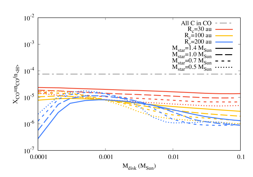
Figure 5: Total disk abundance of CO in the disks of different characteristic radii $R_{\rm c}$ and around stars of different masses, $\gamma=0.5$, at the age of 3 Myr. Line color indicates $R_{\rm c}$, line styles (solid, dashed and dotted) indicate star mass. Maximum $X_{\rm CO}$ is shown with the gray line.

In this section, we use the grid of models to investigate how the various parameters influence the CO abundance in the disk individually. For that purpose, we fix some parameters and check how the results change due to variations in other parameters.

Fig. 5 illustrates the influence of the disk radius and the stellar mass onto the scatter of CO total abundance at a fixed value $\gamma=0.5$. The star mass has only a small impact on the derived CO abundance in compact disks ($R_{\rm c}=30$ au). When we vary $M_{\star}$ between 0.5 and 1.4 $M_{\sun}$, the CO total abundance in compact disks varies only by about a factor of 3, and the higher the star mass is, the larger the CO abundance is. The influence of the star mass becomes more dramatic in disks of larger radii, at least, at the lower end of the considered disk mass range. Here the same variation in $M_{\star}$ leads to an order of magnitude difference in $X_{\rm CO}$. The overall uncertainty of the CO content reaches two orders of magnitude in the least massive disks.

It is also interesting to note that in models with lower disk masses a hotter star leads to a smaller CO abundance, while in models with higher disk masses the opposite trend is observed. Obviously, the CO abundance is limited by the photo-dissociation and photo-desorption, and in various situations the higher star temperature can lead to either decrease or increase in the gas-phase CO abundance. Very low-mass disks, being more transparent for stellar UV-radiation, suffer from CO photo-destruction, which is stronger in disks around more massive stars. Thus, these disks contain less gas-phase CO. Low-mass disks with $R_{\rm c}=30$ au do not show this trend because they encompass the same mass in a more compact region, which results in higher densities and lower influence of photo-dissociation. In massive disks photo-dissociation is not that crucial, and CO depletion is mostly caused by chemical redistribution into ices, especially CO₂ ice. A less massive star causes a CO₂ snowline closer to the star, expanding the zone where CO is effectively removed by chemical processes.

Other considered values of $\gamma$ (0.8, 1.0 and 1.5) do not produce such a high variance in CO total abundance, with larger $\gamma$ giving more stable result. The differences described above, are the highest in disks with $\gamma=0.5$, where surface density falls off slowly, leaving more material in the outer regions of the disk, where CO depletion is stronger. The dependence on $R_{\rm c}$ is caused by a similar effect: disks of equal mass have more matter in the warm inner region if their radii are small, allowing more CO to reside in the gas phase. When $R_{\rm c}$ is large, more mass is in the cold outer area with high CO depletion.

3.4 Initial C/O ratio

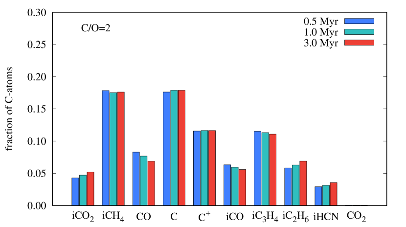
Figure 6: Same as Fig. 3, but for C/O = 2.

The spatial distribution of carbon described in Section 3.2 was computed for a disk with low-metallicity initial composition (Table 1), where there is more oxygen than carbon (C/O$\approx$0.4). To test the effect of other possible elemental compositions we run $200$ models, reducing the initial O abundance from $1.76\times 10^{-4}$ to $3.65\times 10^{-5}$ (leading to C/O = 2).

Fig. 6 presents the fraction of carbon atoms locked up in the various species, dominant in the disk at the previous value of C/O. Compared to Fig. 3, the abundances of CO₂ and CO both in the gas and ice dropped significantly because of the lack of oxygen. On average, only $\sim$7% of C is now in CO gas, while the amount of CO ice stays nearly the same.

Instead of CO₂ ice we have a richer carbon chemistry on dust surfaces. In addition to ices iCH₄, iC₂H₆ and iC₃H₄ we end up with much higher abundances of molecules like iC₅H₂, iCH₃CN, iC₉H₂, iCH₃C₃N and many other surface species with long C chains (Herbst & van Dishoeck, 2009). Abundances of atomic and ionized carbon are also higher compared to the case of C/O=0.4.

Overall, the carbon distribution among species and the abundance of CO depend on initial elemental composition as well.

For the present set of models we have calculated the scatter parameter $s$ as well. The CO scatter parameter is still close to the top with the value of 0.22, it goes again after N₂ with $s=0.20$, and few minor species having the same values of scatter but low mean abundances ($<10^{-9}$). For this elemental composition CO₂, previously showing a low scatter, has $s=0.60$, which worsens its applicability as a mass tracer. Among top species only CO and N₂ retain approximately the same values of scatter at C/O=2.

4 Discussion

While observations of molecular lines remain the only tool to determine gas masses of protoplanetary disks, their interpretation is far from being easy. Even though the most common mass tracer in the interstellar and circumstellar medium, CO, is believed to be controlled by a relatively simple set of processes, its straightforward application to gas mass determination in protoplanetary disks has produced results, which contradict both dust observations and HD observations (Bergin et al., 2013; Favre et al., 2013; McClure et al., 2016). The discrepancy between dust-derived and CO-derived disk masses can in principle be explained by the dust evolution and gas dispersal, but it is harder to reconcile data on various molecular gas mass tracers, like CO and HD, though this difference can be reduced by accounting for CO isotope selection and carbon underabundance in disks, as Trapman et al. (2017) suggest.

The basic assumption behind the possibility of using CO as a mass tracer is that its abundance in protoplanetary disks is defined by the balance between photo-dissociation and freeze-out. Williams & Best (2014) suggested a grid of models based on the assumption that CO is frozen out everywhere, where the temperature is below 20 K, and is photo-dissociated above the H₂ column density of $1.3\times 10^{21}$ cm^-2. If none of these conditions is met, CO is assumed to have the ‘interstellar’ abundance of $10^{-4}$. It becomes increasingly clear that simple prescriptions, like the one suggested by Williams & Best (2014), can produce spurious results. First, as Williams & Best (2014) already noted, more efficient depletion pathways are possible rather than simple CO ice formation. Also, the CO sublimation temperature depends on pressure and under conditions of the disk midplane could be higher than 20 K (Harsono et al., 2015). Second, a typical ‘interstellar’ CO abundance (inherited by the disks) can be lower than $10^{-4}$ (Burgh et al., 2007). One way to infer CO/H₂ ratio in protoplanetary disks directly is to observe absorption lines of both components in the UV band France et al. (2014). This can be one of prospectives for future space UV missions like WSO-Spectrum UV (Boyarchuk et al., 2016) and LUVOIR.

Obviously, more sophisticated methods should be used to infer the total gas mass from CO (or other molecule) observations. In a number of recent papers the utility of CO as a mass tracer has been assessed by means of detailed models of the disk physical and chemical structure. In a series of works by Miotello et al. (2014, 2016, 2017) a disk chemical model with isotope-selective processes was considered in order to find a way to determine the disk mass from CO isotopologue line observations. A large set of disk models was employed to study the evolution of ¹³CO, C¹⁷O, and C¹⁸O in these disks. It was concluded that CO observations can lead to underestimating gas masses in those disks where dust grains have grown to larger sizes. Application of the results to real observations produced very low gas masses in T Tauri disks, often lower than 1 $M_{\rm J}$. It was noted that this can be an effect of sequestering carbon atoms to more complex molecules. This option has not been considered in the above study, as the used chemical model included only a limited set of surface processes (simple hydrogenation processes). The consequence can be seen in Figure 2 from Miotello et al. (2014), where the CO depletion zone is delineated by a $T=20$ K line, and the CO snowline is located at about 100 au.

A more detailed consideration of surface processes was performed by Reboussin et al. (2015). A single surface density distribution was considered in this study, but with different vertical temperature profiles. It was shown that surface conversion of CO into other ices, primarily CO₂ ice, leads to gas-phase CO abundances much lower than the canonical value of $10^{-4}$. Abundances that high are only reached in relatively warm disks with midplane temperatures above 30 K beyond $R=100$ au. In this work results were presented only for the outer part of the disk ($R=100$ and 300 au), where theoretical CO abundance can be quite sensitive to details of radiation transfer (see our results above and also observations presented in Huang et al., 2016).

A chemical evolution with a detailed account of surface reactions and carbon isotope-selective processes was considered by Yu et al. (2016, 2017). They studied the chemical evolution of a typical disk within inner 70 au and found that due to chemical depletion, i.e. conversion of CO into less volatile molecules, the effective CO snowline is located at about 20 au and moves toward the star as the disk evolves, even though the temperature in their model is above the CO sublimation point everywhere in the considered region. According to their results, after 3 Myr of evolution 13.6% of all available carbon is locked in gas-phase CO, while CO₂ ice contains 36.2% of carbon atoms, which compares favorably with our results for a similar disk model (we must note that this agreement is reached despite quite different assumptions on dust properties). While the average value of carbon partition matches well, its dispersion is significant in our modeling (from a few per cent up to 50%). They also found that CO abundance varies with time significantly, which is something that we do not see in our model. However, in their model they vary stellar properties with time, while we keep them constant. The overall conclusion of Yu et al. (2017) is that straightforward interpretation of CO observations leads to underestimation of disk masses. Thus, all the conclusions on the gas deficit in protoplanetary disks based on CO observations should be considered with caution.

The focus of the above studies was on isotope-selective processes and on the usage of CO isotopologue line ratios as mass indicators. In our study we consider CO as a whole, without distinguishing between its isotopologues, concentrating rather on global chemical aspects of CO distributions in disks having different structural parameters.

In our study we consider a wide range of disk sizes, masses, and surface density profiles, assuming that there is no dust evolution, so that dust still has its interstellar parameters. Our results indicate that CO is not an ideal mass tracer, but all other molecules show greater uncertainties in relative abundance. Still, some of them, e.g. H₂O, H₂CO and especially CO₂ can be used as supplementary tracers, particularly, if some information on the disk structure is available.

A better calibration of CO observations can be obtained using the Williams & Best (2014) method, assuming a factor of a few lower typical abundance and taking into account the chemical depletion (e.g., taking 40 K as CO depletion temperature).

An obvious extension of the study is to consider the dependence of our results on the assumed grain size as dust is expected to grow in protoplanetary disks. Akimkin et al. (2013) have shown that the effect of grain growth at its initial stage is to shift the molecular layer closer to the dense midplane. We may provisionally expect that this is going to make molecules better gas mass tracers, but this is a subject for the future study.

5 Conclusions

We conducted a chemical modeling of $\sim 1000$ protoplanetary disk structures around low-mass stars with different parameters to find out species that have the best correlation with the total disk mass. We varied the central star mass, the disk characteristic radius, the disk mass, and $\gamma$-index of surface density distribution, assuming MRN grain size distribution for the UV radiation transfer in the disk atmosphere and 0.1$\mu$m-size grains for the surface chemistry. The chemical modeling is based on the updated non-equilibrium chemical network ALCHEMIC (Semenov & Wiebe, 2011) incorporated into the ANDES code (Akimkin et al., 2013). We focused on an intrinsic dispersion of species abundance due to unknown structural and thermal parameters. The main conclusions are:

– among all 650 considered species, the relative abundance of the CO molecule has one of the smallest scatter in the overall disk ensemble (with obvious exceptions of hydrogen and helium). The characteristic reference ‘$1\sigma$’-values for the logarithm of species total disk abundance at an age of 3 Myr are 0.28 dex for CO and CO₂, 0.29 dex for H₂CO, 0.51 dex for H₂O (see Table 3 for other species). So, even in the case of CO, there is a maximum uncertainty of 1 order of magnitude in CO abundance if the disk physical structure is unknown. More reliable CO disk masses can be obtained if the disk characteristic radius $R_{\rm c}$ is determined.

– on average in the whole disk ensemble, $\approx$ 13% of carbon atoms end up in the gas-phase CO molecule (for the initial ‘low-metals’ abundance from Lee et al. (1998) where C/O = 0.4). The average value of carbon partitioning is in a good agreement with conclusions by Yu et al. (2016). However, the extreme values vary from $\approx$ 2% for large and massive disks to $\approx$ 30% for compact disks with small and moderate masses. Statistically, the most abundant carbon-bearing species is CO₂-ice with average C-atom fraction of $\approx 25\%$. The majority of the remaining carbon atoms are in CH₄ and CO ices (17% and 7% of C-atoms, respectively), C and C⁺ (14% and 8%) and ices of complex organic species. The degree of carbon atom redistribution into non-CO molecules is naturally more effective if C/O $>1$. Quantitatively, the average carbon partition into CO is 7% for C/O = 2.

– despite CO has a noticeable variance in the relative abundance, it is still the best molecular tracer of disk gas mass. The typical value of total CO/H₂ abundance ratio is $1.6\times 10^{-5}$ with ‘$1\sigma$’-limits from $0.8\times 10^{-5}$ to $3.0\times 10^{-5}$. CO₂ also has a low abundance variance, though this variance depends strongly on C/O ratio. Other species that have relatively good correlation with disk mass are H₂O and H₂CO.

We find that on average the total abundance of gaseous CO in protoplanetary disks is $\approx$ 6 times lower compared to the interstellar value of $10^{-4}$. Chemical depletion lowers the abundance of CO by a factor of 3, compared to the case of photo-dissociation and freeze-out as the only ways of CO destruction.

Appendix A Ice species

Here we present the version of Table 3 for ice species. Table 4 lists ice species with average total abundance in the disk above $10^{-11}$ sorted by the scatter.

Table 4: Average total abundance $\overline{X_{i}}=10^{\overline{x_{i}}}$ and scatter $s_{i}$ for ice species.

Species	$\overline{X_{i}}$	$s_{i}$, dex	Species	$\overline{X_{i}}$	$s_{i}$, dex	Species	$\overline{X_{i}}$	$s_{i}$, dex
iSiO	$8.1\times 10^{-10}$	0.20	iCH3CN	$1.1\times 10^{-9}$	0.62	iC6H6	$2.1\times 10^{-11}$	0.94
iCO2	$1.7\times 10^{-5}$	0.26	iC3H4	$6.7\times 10^{-7}$	0.65	iH2S2	$5.1\times 10^{-10}$	0.96
iFeH	$1.9\times 10^{-9}$	0.26	iPO	$1.2\times 10^{-11}$	0.65	iH2CO	$6.6\times 10^{-8}$	0.96
iMgH2	$4.4\times 10^{-9}$	0.28	iHC3N	$2.1\times 10^{-11}$	0.65	iH2	$1.1\times 10^{-7}$	0.96
iC2H4	$3.0\times 10^{-10}$	0.28	iC7H2	$1.9\times 10^{-11}$	0.66	iH2C3O	$4.6\times 10^{-10}$	0.99
iHNC	$1.1\times 10^{-8}$	0.29	iC8H4	$1.0\times 10^{-9}$	0.66	iCH3C4H	$8.0\times 10^{-11}$	1.05
iHNCO	$3.5\times 10^{-9}$	0.34	iC4N	$1.5\times 10^{-11}$	0.67	iNH2CHO	$2.3\times 10^{-9}$	1.10
iSiH4	$3.8\times 10^{-9}$	0.35	iH3C5N	$3.2\times 10^{-11}$	0.69	iCH2CO	$1.7\times 10^{-9}$	1.17
iP	$7.6\times 10^{-11}$	0.36	iCH3OH	$5.2\times 10^{-8}$	0.69	iHNO	$3.3\times 10^{-9}$	1.29
iHCN	$9.8\times 10^{-7}$	0.37	iC8H2	$1.6\times 10^{-11}$	0.70	iO2	$7.6\times 10^{-10}$	1.32
iHCl	$2.4\times 10^{-10}$	0.38	iH5C3N	$2.2\times 10^{-10}$	0.71	iS2	$4.0\times 10^{-10}$	1.38
iC5H2	$3.3\times 10^{-10}$	0.39	iC7H4	$1.9\times 10^{-9}$	0.72	iNH2	$2.3\times 10^{-11}$	1.39
iCl	$2.9\times 10^{-10}$	0.40	iCH4	$5.3\times 10^{-6}$	0.73	iNO	$1.1\times 10^{-11}$	1.49
iH2O	$5.1\times 10^{-5}$	0.40	iC5H4	$7.6\times 10^{-8}$	0.73	iC4H4	$4.3\times 10^{-10}$	1.50
iNaH	$9.5\times 10^{-10}$	0.43	iC2H6	$7.3\times 10^{-7}$	0.74	iCH3OCH3	$1.9\times 10^{-11}$	1.52
iNH3	$6.6\times 10^{-6}$	0.46	iN2H2	$2.3\times 10^{-11}$	0.76	iC2H5OH	$2.0\times 10^{-11}$	1.53
iH2O2	$5.2\times 10^{-8}$	0.49	iH2CS	$4.5\times 10^{-9}$	0.81	iOH	$5.0\times 10^{-10}$	1.56
iC3S	$7.3\times 10^{-11}$	0.49	iHCOOH	$1.6\times 10^{-8}$	0.82	iCH3CHO	$2.3\times 10^{-9}$	1.57
iC6H2	$9.4\times 10^{-11}$	0.49	iC9H4	$2.2\times 10^{-9}$	0.83	iCH3	$3.1\times 10^{-11}$	1.60
iNH2OH	$7.8\times 10^{-10}$	0.53	iCH5N	$9.6\times 10^{-9}$	0.83	iCH2	$3.0\times 10^{-11}$	1.64
iN2	$6.8\times 10^{-7}$	0.55	iC9H2	$6.3\times 10^{-11}$	0.84	iCH	$2.2\times 10^{-11}$	1.75
iCO	$3.2\times 10^{-6}$	0.58	iO3	$2.7\times 10^{-9}$	0.85	iO	$1.3\times 10^{-10}$	1.75
iH2S	$2.3\times 10^{-8}$	0.59	iHS2	$2.3\times 10^{-10}$	0.86	iC	$2.2\times 10^{-11}$	1.86
iC3H2	$1.2\times 10^{-9}$	0.60	iC6H4	$1.8\times 10^{-8}$	0.88	iH	$2.4\times 10^{-9}$	1.98
iC2H2	$9.5\times 10^{-11}$	0.61	iN2O	$1.1\times 10^{-11}$	0.92

References

- Akimkin et al. (2013) Akimkin, V., Zhukovska, S., Wiebe, D., et al. 2013, ApJ, 766, 8
- Akimkin (2015) Akimkin, V. V. 2015, Astronomy Reports, 59, 747
- Andrews & Williams (2005) Andrews, S. M., & Williams, J. P. 2005, ApJ, 631, 1134
- Ansdell et al. (2017) Ansdell, M., Williams, J. P., Manara, C. F., et al. 2017, AJ, 153, 240
- Ansdell et al. (2016) Ansdell, M., Williams, J. P., van der Marel, N., et al. 2016, ApJ, 828, 46
- Armitage (2015) Armitage, P. J. 2015, arXiv preprint arXiv:1509.06382
- Bai & Goodman (2009) Bai, X.-N., & Goodman, J. 2009, ApJ, 701, 737
- Baraffe et al. (2015) Baraffe, I., Homeier, D., Allard, F., & Chabrier, G. 2015, A&A, 577, A42
- Bergin et al. (2010) Bergin, E. A., Hogerheijde, M. R., Brinch, C., et al. 2010, A&A, 521, L33
- Bergin et al. (2013) Bergin, E. A., Cleeves, L. I., Gorti, U., et al. 2013, Nature, 493, 644
- Bitsch et al. (2015) Bitsch, B., Lambrechts, M., & Johansen, A. 2015, A&A, 582, A112
- Bohlin et al. (1978) Bohlin, R. C., Savage, B. D., & Drake, J. F. 1978, ApJ, 224, 132
- Bolatto et al. (2013) Bolatto, A. D., Wolfire, M., & Leroy, A. K. 2013, ARA&A, 51, 207
- Boyarchuk et al. (2016) Boyarchuk, A. A., Shustov, B. M., Savanov, I. S., et al. 2016, Astronomy Reports, 60, 1
- Burgh et al. (2007) Burgh, E. B., France, K., & McCandliss, S. R. 2007, ApJ, 658, 446
- Carmona et al. (2011) Carmona, A., van der Plas, G., van den Ancker, M. E., et al. 2011, A&A, 533, A39
- Chapillon et al. (2012) Chapillon, E., Guilloteau, S., Dutrey, A., Piétu, V., & Guélin, M. 2012, A&A, 537, A60
- Chapillon et al. (2011) Chapillon, E., Parise, B., Guilloteau, S., & Du, F. 2011, A&A, 533, A143
- Chiang & Goldreich (1997) Chiang, E. I., & Goldreich, P. 1997, ApJ, 490, 368
- Dartois et al. (2003) Dartois, E., Dutrey, A., & Guilloteau, S. 2003, A&A, 399, 773
- Draine (2006) Draine, B. T. 2006, ApJ, 636, 1114
- Dullemond & Dominik (2004) Dullemond, C. P., & Dominik, C. 2004, A&A, 421, 1075
- Dullemond et al. (2001) Dullemond, C. P., Dominik, C., & Natta, A. 2001, ApJ, 560, 957
- Dunham et al. (2014) Dunham, M. M., Vorobyov, E. I., & Arce, H. G. 2014, MNRAS, 444, 887
- Dutrey et al. (1997) Dutrey, A., Guilloteau, S., & Guelin, M. 1997, A&A, 317, L55
- Dutrey et al. (2011) Dutrey, A., Wakelam, V., Boehler, Y., et al. 2011, A&A, 535, A104
- Favre et al. (2013) Favre, C., Cleeves, L. I., Bergin, E. A., Qi, C., & Blake, G. A. 2013, ApJ, 776, L38
- France et al. (2014) France, K., Herczeg, G. J., McJunkin, M., & Penton, S. V. 2014, ApJ, 794, 160
- Goldsmith et al. (1997) Goldsmith, P. F., Bergin, E. A., & Lis, D. C. 1997, ApJ, 491, 615
- Guilloteau et al. (2016) Guilloteau, S., Reboussin, L., Dutrey, A., et al. 2016, A&A, 592, A124
- Harsono et al. (2015) Harsono, D., Bruderer, S., & van Dishoeck, E. F. 2015, A&A, 582, A41
- Hartmann et al. (1998) Hartmann, L., Calvet, N., Gullbring, E., & D’Alessio, P. 1998, ApJ, 495, 385
- Hässig et al. (2015) Hässig, M., Altwegg, K., Balsiger, H., et al. 2015, Science, 347, aaa0276
- Henning & Meeus (2011) Henning, T., & Meeus, G. 2011, Dust Processing and Mineralogy in Protoplanetary Accretion Disks, ed. P. J. V. Garcia, 114–148
- Henning & Semenov (2008) Henning, T., & Semenov, D. 2008, in IAU Symposium, Vol. 251, Organic Matter in Space, ed. S. Kwok & S. Sanford, 89–98
- Henning & Semenov (2013) Henning, T., & Semenov, D. 2013, Chemical Reviews, 113, 9016
- Herbst & van Dishoeck (2009) Herbst, E., & van Dishoeck, E. F. 2009, ARA&A, 47, 427
- Hogerheijde et al. (2011) Hogerheijde, M. R., Bergin, E. A., Brinch, C., et al. 2011, Science, 334, 338
- Huang et al. (2016) Huang, J., Öberg, K. I., & Andrews, S. M. 2016, ApJ, 823, L18
- Isella et al. (2016) Isella, A., Guidi, G., Testi, L., et al. 2016, Physical Review Letters, 117, 251101
- Ivlev et al. (2016) Ivlev, A. V., Akimkin, V. V., & Caselli, P. 2016, ApJ, 833, 92
- Laor & Draine (1993) Laor, A., & Draine, B. T. 1993, ApJ, 402, 441
- Lee et al. (1998) Lee, H.-H., Roueff, E., Pineau des Forets, G., et al. 1998, A&A, 334, 1047
- Loomis et al. (2015) Loomis, R. A., Cleeves, L. I., Öberg, K. I., Guzman, V. V., & Andrews, S. M. 2015, ApJ, 809, L25
- Mathis et al. (1983) Mathis, J. S., Mezger, P. G., & Panagia, N. 1983, A&A, 128, 212
- Mathis et al. (1977) Mathis, J. S., Rumpl, W., & Nordsieck, K. H. 1977, ApJ, 217, 425
- McClure et al. (2016) McClure, M. K., Bergin, E. A., Cleeves, L. I., et al. 2016, ApJ, 831, 167
- Miotello et al. (2014) Miotello, A., Bruderer, S., & van Dishoeck, E. F. 2014, A&A, 572, A96
- Miotello et al. (2016) Miotello, A., van Dishoeck, E. F., Kama, M., & Bruderer, S. 2016, A&A, 594, A85
- Miotello et al. (2017) Miotello, A., van Dishoeck, E. F., Williams, J. P., et al. 2017, A&A, 599, A113
- Mordasini et al. (2012) Mordasini, C., Alibert, Y., Benz, W., Klahr, H., & Henning, T. 2012, A&A, 541, A97
- Mumma & Charnley (2011) Mumma, M. J., & Charnley, S. B. 2011, ARA&A, 49, 471
- Öberg et al. (2015) Öberg, K. I., Guzmán, V. V., Furuya, K., et al. 2015, Nature, 520, 198
- Öberg et al. (2017) Öberg, K. I., Guzmán, V. V., Merchantz, C. J., et al. 2017, ApJ, 839, 43
- Okuzumi (2009) Okuzumi, S. 2009, ApJ, 698, 1122
- Qi et al. (2011) Qi, C., D’Alessio, P., Öberg, K. I., et al. 2011, ApJ, 740, 84
- Qi et al. (2013) Qi, C., Öberg, K. I., & Wilner, D. J. 2013, ApJ, 765, 34
- Rab et al. (2017) Rab, C., Elbakyan, V., Vorobyov, E., et al. 2017, ArXiv e-prints, arXiv:1705.03946
- Reboussin et al. (2015) Reboussin, L., Wakelam, V., Guilloteau, S., Hersant, F., & Dutrey, A. 2015, A&A, 579, A82
- Salinas et al. (2016) Salinas, V. N., Hogerheijde, M. R., Bergin, E. A., et al. 2016, A&A, 591, A122
- Sano et al. (2000) Sano, T., Miyama, S. M., Umebayashi, T., & Nakano, T. 2000, ApJ, 543, 486
- Semenov & Wiebe (2011) Semenov, D., & Wiebe, D. 2011, ApJS, 196, 25
- Semenov et al. (2006) Semenov, D., Wiebe, D., & Henning, T. 2006, ApJ, 647, L57
- Thi et al. (2011) Thi, W.-F., Ménard, F., Meeus, G., et al. 2011, A&A, 530, L2
- Trapman et al. (2017) Trapman, L., Miotello, A., Kama, M., van Dishoeck, E. F., & Bruderer, S. 2017, ArXiv e-prints, arXiv:1705.07671
- Tsukamoto et al. (2017) Tsukamoto, Y., Okuzumi, S., & Kataoka, A. 2017, ApJ, 838, 151
- Vasyunin et al. (2017) Vasyunin, A. I., Caselli, P., Dulieu, F., & Jiménez-Serra, I. 2017, ApJ, 842, 33
- Vasyunina et al. (2012) Vasyunina, T., Vasyunin, A. I., Herbst, E., & Linz, H. 2012, ApJ, 751, 105
- Wakelam et al. (2015) Wakelam, V., Loison, J.-C., Herbst, E., et al. 2015, ApJS, 217, 20
- Walsh et al. (2016) Walsh, C., Loomis, R. A., Öberg, K. I., et al. 2016, ApJ, 823, L10
- Williams & Best (2014) Williams, J. P., & Best, W. M. J. 2014, ApJ, 788, 59
- Williams & Cieza (2011) Williams, J. P., & Cieza, L. A. 2011, ARA&A, 49, 67
- Williams & McPartland (2016) Williams, J. P., & McPartland, C. 2016, ApJ, 830, 32
- Yu et al. (2017) Yu, M., Evans, II, N. J., Dodson-Robinson, S. E., Willacy, K., & Turner, N. J. 2017, ApJ, 841, 39
- Yu et al. (2016) Yu, M., Willacy, K., Dodson-Robinson, S. E., Turner, N. J., & Evans, II, N. J. 2016, ApJ, 822, 53
- Zhang et al. (2017) Zhang, K., Bergin, E. A., Blake, G. A., Cleeves, L. I., & Schwarz, K. R. 2017, Nature Astronomy, 1, 0130