Virtual-Voltage Partition-Based Approach to Optimal Transmission Switching

Abstract

This paper deals with optimal transmission switching (OTS) problems involving discrete binary decisions about network topology and non-convex power flow constraints. We adopt a semidefinite programming formulation for the OPF problem which, however, remains nonconvex due to the presence of discrete variables and bilinear products between the decision variables. To tackle the latter, we introduce a novel physically-inspired, virtual-voltage approximation that leads to provable lower and upper bounds on the solution of the original problem. To deal with the exponential complexity caused by the discrete variables, we introduce a graph partition-based algorithm which breaks the problem into several parallel mixed-integer subproblems of smaller size. Simulations demonstrate the high degree of accuracy and affordable computational requirements of our approach.

I Introduction

Optimal transmission switching (OTS) is concerned with the identification of power grid topologies that minimize generation cost while maintaining the secure operation of the grid. This leads to a class of non-convex optimization problems with discrete decision variables and bilinear constraints. Solving OTS has the potential to yield significant benefits in efficiency and reliability while respecting security constraints, but the complexity of solving such highly non-convex problems makes achieving this goal difficult. Our focus here is on developing a computationally efficient approach to approximate the solution of OTS problems.

Literature review: Discrete variables appear in optimal power flow (OPF) problems in many ways, such as transmission switching and post-contingency controls. The works [2, 3, 4] provide surveys on the solution of OPF problems with discrete variables. Many of the methods employed to solve OPF problems have been extended to deal with mixed-integer OPF, e.g., particle swarm optimization [5, 6] and genetic algorithms [7]. Transmission line switching or network topology reconfiguration commonly serve as corrective mechanisms in response to system contingencies see [8, 9] and references therein. In [10, 11, 12], linearized OPF, also known as DCOPF, is deployed to solve OTS efficiently. Despite its relative low complexity, DCOPF may lead, especially in congested systems, to poor solutions that can even result in voltage collapse [13, 14]. The work [15] proposes quadratic convex (QC) relaxations for the MIP-OPF problem, which provides more accurate results than DCOPF, while still retaining a fast computation time. Recent studies [15, 16] show that methods based on semidefinite programming (SDP) convex relaxations of ACOPF may lead to better solutions than DCOPF and QC. However, how to handle variables for transmission switching in the context of SDP is challenging and not fully understood. The challenges stem from not only from the integer-valued nature of these variables, but also from the presence of bilinear terms involving the product of discrete decision variables with continuous ones, reflecting the impact on the physical modeling of the line being connected. The paper [16] uses a lift-and-branch-and-bound procedure to deal with the SDP formulation of mixed-integer OPF (OTS as a special case), but has still exponential complexity in the worst case due to the nature of the branch-and-bound procedure. The work [17] also uses SDP to solve OTS problems, where bilinear terms associated to line connections are addressed by assuming certain nominal network topology and bilinear terms of other discrete decision variables are dealt with using the McCormick relaxation [18].

Statement of contributions: We consider the OTS problem and introduce a novel SDP convex relaxation to approximate its solution. Our contributions are twofold. First, we introduce a novel way of dealing with the nonconvexity coming from the presence of bilinear terms, which we term virtual-voltage approximation. Our approach is based on introducing virtual-voltage variables for the terminal nodes of each switchable line and impose physically-meaningful constraints on them. We show that this approach leads to sound bounds on individual flows of the switchable lines, and provides lower and upper bounds on the optimal value of the original problem. Our second contribution deals with the nonconvexity coming from the discrete variables. We build on the virtual-voltage approximation to propose a graph partition-based algorithm that significantly reduces the computational complexity of solving the original problem. This algorithm uses the values of the optimal dual variables from the virtual-voltage method to define a weighted network graph, which is then partitioned with a minimum weight edge-cut set. The algorithm breaks the original network into sub-networks so as to minimize the correlation between the solutions to the optimization problem on each sub-network. Finally, the algorithm solves the OTS problem on each sub-network in parallel and combines them to reconstruct the solution of the original problem. We implement the proposed algorithms on various IEEE standard test cases, and compare them with available approaches from the literature to illustrate their superior performance regarding convergence to the optima and computation time.

II Preliminaries

This section introduces basic concepts used in the paper.

II-1 Graph Theory

We review basic notions of graph theory following [19]. A graph is a pair $\operatorname{\mathcal{G}}=(\operatorname{\mathcal{N}},\operatorname{\mathcal{E}})$, where $\operatorname{\mathcal{N}}\subseteq\operatorname{\mathbb{N}}$ is the set of nodes and $\operatorname{\mathcal{E}}\subseteq\operatorname{\mathcal{N}}\times\operatorname{\mathcal{N}}$ is the set of edges. A self-loop is an edge that connects a node to itself. The graph is undirected if $\{i,k\}=\{k,i\}\in\operatorname{\mathcal{E}}$. A path is a sequence of nodes such that any two consecutive nodes correspond to an edge. The graph is connected if there exists a path between any two nodes. An orientation of an undirected graph is an assignment of exactly one direction to each of its edges. A graph is simple if it does not have self-loops or multiple edges connecting any pair of nodes. Throughout the paper, we limit our discussion to undirected, simple graphs. A vertex-induced subgraph of $\operatorname{\mathcal{G}}$, written $\operatorname{\mathcal{G}}[\operatorname{\mathcal{N}}_{s}]=(\operatorname{\mathcal{N}}_{s},\operatorname{\mathcal{E}}_{s})$, satisfies $\operatorname{\mathcal{N}}_{s}\subseteq\operatorname{\mathcal{N}}$ and $\operatorname{\mathcal{E}}_{s}=\operatorname{\mathcal{E}}\cap(\operatorname{\mathcal{N}}_{s}\times\operatorname{\mathcal{N}}_{s})$. An edge cut set is a subset of edges which, if removed, disconnects the graph. A weighted graph is a graph where each branch $\{i,k\}$ has a weight, $w_{ik}\in_{+}$. Given the edge weights $w\in_{+}^{|\operatorname{\mathcal{E}}|}$, the adjacency matrix $A$ has $A(i,k)=A(k,i)=w_{ik}$ if $\{i,k\}\in\operatorname{\mathcal{E}}$, and $A(i,k)=0$ otherwise. The degree matrix $D$ is a diagonal matrix such that $D(i,i)=\sum_{k,\{i,k\}\in\operatorname{\mathcal{E}}}w_{ik}$. The normalized adjacency matrix is $A_{n}=\sqrt{D}^{-1}A\sqrt{D}^{-1}$. The Laplacian matrix is $L=D-A$. The Laplacian matrix is positive semidefinite, with zero as an eigenvalue and multiplicity equal to the number of connected components in the graph. The Fiedler vector is the eigenvector associated with the second smallest eigenvalue of $L$. An $n$-partition of a connected $\operatorname{\mathcal{G}}=(\operatorname{\mathcal{N}},\operatorname{\mathcal{E}},A)$ divides $\operatorname{\mathcal{G}}$ into a number of $n$ connected vertex-induced subgraphs, $\operatorname{\mathcal{G}}[\operatorname{\mathcal{V}}_{i}]$, such that $\cup_{i=1}^{n}\operatorname{\mathcal{V}}_{i}=\operatorname{\mathcal{N}}$ and $\operatorname{\mathcal{V}}_{i}\cap\operatorname{\mathcal{V}}_{k}=\emptyset$ for all $i\neq k$. An $n$-optimal partition of $\operatorname{\mathcal{G}}=(\operatorname{\mathcal{N}},\operatorname{\mathcal{E}},A)$ is an $n$-partition of $\operatorname{\mathcal{G}}$ with $\sum_{\{i,k\}\in\operatorname{\mathcal{E}}_{c}}w_{ik}$ minimized, where $\operatorname{\mathcal{E}}_{c}=\operatorname{\mathcal{E}}\setminus(\cup_{i=1}^{n}\operatorname{\mathcal{V}}_{i}\times\operatorname{\mathcal{V}}_{i})$. Spectral graph partitioning partitions a connected graph $\operatorname{\mathcal{G}}$ into two vertex-induced subgraphs, $\operatorname{\mathcal{G}}[\operatorname{\mathcal{N}}_{1}]$ and $\operatorname{\mathcal{G}}[\operatorname{\mathcal{N}}_{2}]$, where $\operatorname{\mathcal{N}}_{1}$ and $\operatorname{\mathcal{N}}_{2}$ are the nodes corresponding to the positive and non-positive entries of the Fiedler vector, respectively.

II-2 McCormick Relaxation of Bilinear Terms

The McCormick envelopes [18] provide linear relaxations for optimization problems that involve bilinear terms. Consider a bilinear term $xy$ on the variables $x,y\in$, for which there exist upper and lower bounds, $\underline{x}\leq x\leq\overline{x},\quad\underline{y}\leq y\leq\overline{y}$. The McCormick relaxation consists of substituting in the optimization problem the term $xy$ by its surrogate $v\in$ and adding the following McCormick envelopes on $v$,

$$v\geq\underline{x}y+x\underline{y}-\underline{x}\underline{y},\quad v\geq\overline{x}y+x\overline{y}-\overline{x}\overline{y},$$ (1a)

$$v\leq\overline{x}y+x\underline{y}-\overline{x}\underline{y},\quad v\leq x\overline{y}+\underline{x}y-\underline{x}\overline{y}.$$ (1b)

Constraints (1) are tight, in the sense that each plane in (1) is tangent to the bilinear-constraint manifold at two boundary lines. The convex polyhedron in the variables $(x,y,v)$ encloses the actual bilinear-constraint manifold.

III Problem Statement

We begin with the formulation of the OPF problem over an electrical network and its SDP convex relaxation following [20]. Then, we introduce binary variables leading to the OTS problem formulation of interest in this paper.

Consider an electrical network with generation buses $\operatorname{\mathcal{N}}_{G}$, load buses $\operatorname{\mathcal{N}}_{L}$, and electrical interconnections described by an undirected edge set $\operatorname{\mathcal{E}}_{0}$. Let $\operatorname{\mathcal{N}}=\operatorname{\mathcal{N}}_{G}\cup\operatorname{\mathcal{N}}_{L}$ and denote its cardinality by $N$. We denote the phasor voltage at bus $i$ by $V_{i}=E_{i}e^{j\theta_{i}}$, where $E_{i}\in\mathbb{R}$ and $\theta_{i}\in[-\pi,\pi)$ are the voltage magnitude and phase angle, respectively. For convenience, $V=\{V_{i}\;|\;i\in\operatorname{\mathcal{N}}\}$ denotes the collection of voltages at all buses. The active and reactive power injections at bus $i$ are given by the power flow equations

$$P_{i} =\operatorname{\bf Tr}\{Y_{i}VV^{*}\}+P_{D_{i}},\quad Q_{i}=\operatorname{\bf Tr}\{\overline{Y}_{i}VV^{*}\}+Q_{D_{i}},$$ (2)

where $P_{D_{i}},Q_{D_{i}}\in\operatorname{\mathbb{R}}$ are the active and reactive power demands at bus $i$, and $Y_{i},\overline{Y}_{i}\in\mathcal{H}^{N}$ are derived from the admittance matrix Y$\in\mathbb{C}^{N\times N}$ as follows

$$Y_{i} =\frac{(e_{i}e_{i}^{\top}\textbf{Y})^{*}+e_{i}e_{i}^{\top}\textbf{Y}}{2},\quad\overline{Y}_{i}=\frac{(e_{i}e_{i}^{\top}\textbf{Y})^{*}-e_{i}e_{i}^{\top}\textbf{Y}}{2j}.$$ (3a)

Here $\{e_{i}\}_{i=1,\dots,N}$ denotes the canonical basis of ^N. The OPF problem also involves the box constraints

$$\underline{V}_{i}^{2}\leq|V_{i}|^{2}\leq\overline{V}_{i}^{2},\;\forall i\in\mathcal{N},$$

$$\underline{P}_{i}\leq P_{i}\leq\overline{P}_{i},\;\;\underline{Q}_{i}\leq Q_{i}\leq\overline{Q}_{i},\;\forall i\in\mathcal{N},$$ (4)

$$|V_{i}-V_{k}|^{2}\leq\overline{V}_{ik},\;\forall\{i,k\}\in\operatorname{\mathcal{E}}_{0},$$

where $\overline{V}_{ik}$ is the upper bound of the voltage difference between buses $i,k$, and $\underline{V}_{i}$ and $\overline{V}_{i}$ are the lower and upper bounds of the voltage magnitude at bus $i$, respectively. Notice that the upper bound of the voltage difference is equivalent to line thermal constraints, as described for instance in [21]. The voltage difference constraints prevent overheating of transmission lines. All $\underline{P}_{i},\underline{Q}_{i},\overline{P}_{i},\overline{Q}_{i}$, are defined similarly. The objective function is typically given as a quadratic function of the active power,

$$\sum\nolimits_{k\in\mathcal{N}_{G}}c_{i2}P_{i}^{2}+c_{i1}P_{i},$$ (5)

where $c_{i2}\geq 0$, and $c_{i1}\in\mathbb{R}$. The OPF problem is the minimization over (5) subject to (2) and (III). Such optimization is non-convex due to the quadratic terms on $V$. To address this, one can equivalently define $W=VV^{*}\in\mathcal{H}^{N}$ (or $W\in\mathcal{H}^{N}$ and $\operatorname{rank}(W)=1$) as the decision variable (note all the terms in (2), (III) and (5) are quadratic in $V$). Dropping the rank constraint on $W$ makes the OPF problem convex, giving rise to the SDP convex relaxation,

$$\textbf{(P1)}\hskip 42.67912pt\min_{W\succeq 0}\sum\nolimits_{i\in\operatorname{\mathcal{N}}_{G}}c_{i2}P_{i}^{2}+c_{i1}P_{i},$$

subject to

$$P_{i}=\operatorname{\bf Tr}\{Y_{i}W\}+P_{D_{i}},\;\forall i\in\mathcal{N},$$ (6a)

$$Q_{i}=\operatorname{\bf Tr}\{\overline{Y}_{i}W\}+Q_{D_{i}},\;\forall i\in\mathcal{N},$$ (6b)

$$\underline{P}_{i}\leq P_{i}\leq\overline{P}_{i},\;\underline{Q}_{i}\leq Q_{i}\leq\overline{Q}_{i},\;\;\forall i\in\mathcal{N},$$ (6c)

$$\underline{V}_{i}^{2}\leq\operatorname{\bf Tr}\{M_{i}W\}\leq\overline{V}_{i}^{2},\;\forall i\in\mathcal{N},$$ (6d)

$$\operatorname{\bf Tr}\{M_{ik}W\}\leq\overline{V}_{ik},\;\forall\{i,k\}\in\operatorname{\mathcal{E}}_{0},$$ (6e)

where $M_{i},M_{ik}\in\mathcal{H}^{N}$ are defined so that $\operatorname{\bf Tr}\{M_{i}W\}=|V_{i}|^{2}$ and $\operatorname{\bf Tr}\{M_{ik}W\}=|V_{i}-V_{k}|^{2}$.

In the OTS problem, the set of transmission lines $\operatorname{\mathcal{E}}_{0}$ is divided into a set of switchable $\operatorname{\mathcal{E}}_{s}$ and non-switchable $\operatorname{\mathcal{E}}$ lines such that $\operatorname{\mathcal{E}}_{0}=\operatorname{\mathcal{E}}_{s}\cup\operatorname{\mathcal{E}}$ (note that $\operatorname{\mathcal{E}}_{s}=\operatorname{\mathcal{E}}_{0}$ and $\operatorname{\mathcal{E}}=\emptyset$ is possible). Choosing among the switchable lines which ones are active affects the nodal active and reactive power injections in (6c). The question is then to determine what the optimal choice of switching lines is. We formalize this problem next. For each line $\{i,k\}\in\operatorname{\mathcal{E}}_{s}$, we define a binary variable $\alpha_{ik}\in\{0,1\}$, and we say the line is connected if $\alpha_{ik}=1$ and disconnected otherwise. If $\alpha_{ik}=1$, then the power flow from node $i$ to $k$ through edge $\{i,k\}\in\operatorname{\mathcal{E}}_{s}$ is

$$P_{ik}=\operatorname{\bf Tr}\{Y_{ik}W\},\quad Q_{ik}=\operatorname{\bf Tr}\{\overline{Y}_{ik}W\},$$ (7)

where $Y_{ik},\overline{Y}_{ik}\in\operatorname{\mathbb{C}}^{N\times N}$ are defined as follows: all entries are prescribed to be zero except the ones defined by

$$Y_{ik}(i,i) =\Re(y_{ik}),\quad Y_{ik}(i,k)=Y^{*}_{ik}(i,k)=-y_{ik}/2,$$

$$\overline{Y}_{ik}(i,i) =\Im(y_{ik}),\quad\overline{Y}_{ik}(i,k)=\overline{Y}^{*}_{ik}(i,k)=-j\cdot y_{ik}/2.$$

Here $y_{ik}\in\mathbb{C}$ is the admittance of line $\{i,k\}$. Taking (7) into account, the active and reactive power of each node become

$$P_{i}=\operatorname{\bf Tr}\{Y_{i}W\}+P_{D_{i}}+\sum\nolimits_{k\in\operatorname{\mathcal{S}}_{i}}\alpha_{ik}P_{ik},$$ (8)

$$Q_{i}=\operatorname{\bf Tr}\{\overline{Y}_{i}W\}+Q_{D_{i}}+\sum\nolimits_{k\in\operatorname{\mathcal{S}}_{i}}\alpha_{ik}Q_{ik},$$

where $\operatorname{\mathcal{S}}_{i}:=\{k\;|\;\{i,k\}\in\operatorname{\mathcal{E}}_{s}\}$. Given $\alpha\in\{0,1\}^{|{\operatorname{\mathcal{E}}}_{s}|}$, we use (P1)-$\alpha$ to refer to the OPF problem solved with the network topology with extra lines as determined by $\alpha$.

We are interested in solving what we call (P2), which is the optimization (P1) with constraints (6a) and (6b) replaced by (7) and (8). In addition to the optimization of the power flow, this formulation incorporates the optimal choice among the switchable lines in $\operatorname{\mathcal{E}}_{s}$. The problem (P2) is non-convex for two reasons: the binary variables $\alpha_{ik}$ and the bilinear products of $\alpha_{ik}$ and $W$. The first problem can be addressed using existing integer-programming solvers [22, 17]. The McCormick relaxation described in Section II-2 is the standard way to deal with the second problem. In this paper, we instead provide alternative routes to address each of these problems for the optimization (P2).

Remark III.1.

(Networks where all lines are switchable). General formulations of the OTS problem assume all transmission lines are switchable, see e.g. [23, 15]. Some works also pre-select a pool of switchable lines through heuristic methods [23]. The approach described next is applicable to both types of scenarios. $\square$

IV Virtual-Voltage Approximation of Bilinear Terms

We introduce here a novel way to deal with the bilinear terms in (P2) which we term virtual-voltage approximation. We start by noting that every binary variable $\alpha$ only appears in the bilinear products in (8) together with another continuous variable $W$. If we convexify the binary variables by having them take values in $[0,1]$, then we can interpret each bilinear term corresponding to $\{i,k\}\in\operatorname{\mathcal{E}}_{s}$ as a line power flow from $i$ to $k$, with the magnitude bounded by what $W$ indicates. Following this reasoning, if the direction of power flow of every line $\{i,k\}\in\operatorname{\mathcal{E}}_{s}$ was known, then the bilinear term would no longer be an issue. For example, if we knew that $P_{ik}=\operatorname{\bf Tr}\{Y_{ik}W\}\in_{+}$ and $Q_{ik}=\operatorname{\bf Tr}\{\overline{Y}_{ik}W\}\in_{+}$, then we could define new variables, $\hat{P}_{ik}\in$ and $\hat{Q}_{ik}\in$, replacing $\alpha_{ik}P_{ik}$ and $\alpha_{ik}Q_{ik}$ in (8), respectively, and impose

$$0\leq\hat{P}_{ik}\leq P_{ik},\quad 0\leq\hat{Q}_{ik}\leq Q_{ik}.$$ (9)

This would eliminate the bilinear terms and the only remaining non-convexity would be that the physical feasible solution should satisfy $\hat{P}_{ik}\in\{0,P_{ik}\}$ and $\hat{Q}_{ik}\in\{0,Q_{ik}\}$. In general, however, the direction of power flow of the lines $\{i,k\}\in\operatorname{\mathcal{E}}_{s}$ is not known a priori and, hence, the trivial convex constraints (9) for the relaxation are no longer valid.

IV-A Convex Relaxation Via Virtual Voltages

Our idea to approximate each bilinear term builds on defining a virtual-voltage for the terminal nodes of the line and impose constraints on them to make sure they have physical sense. We make this precise next. Let $\hat{\operatorname{\mathcal{E}}}_{s}$ be an arbitrary orientation of $\operatorname{\mathcal{E}}_{s}$. To define the virtual-voltages, and in keeping with the SDP approach, for each $\{i,k\}\in\hat{\operatorname{\mathcal{E}}}_{s}$ we introduce a two-by-two positive semidefinite matrix $U_{ik}\in\operatorname{\mathbb{S}}^{2}_{+}$. This matrix encodes physically meaningful voltages at the terminal nodes if its rank is one, namely, $U_{ik}=u_{ik}u_{ik}^{\top}$, with $u_{ik}(1)$ and $u_{ik}(2)$ corresponding to the voltages of nodes $i$ and $k$, respectively. For convenience, we introduce $\hat{M}=[\begin{smallmatrix}1&-1\\ -1&1\end{smallmatrix}]$ and impose the following constraints on $U_{ik}$

$$U_{ik}(1,1) \leq\operatorname{\bf Tr}\{M_{i}W\},$$ (10a)

$$U_{ik}(2,2) \leq\operatorname{\bf Tr}\{M_{k}W\},$$ (10b)

$$\operatorname{\bf Tr}\{\hat{M}U_{ik}\} \leq\operatorname{\bf Tr}\{M_{ik}W\}.$$ (10c)

Constraints (10a) and (10b) ensure that the voltage magnitudes of $i$ and $k$ derived from $U_{ik}$ are no bigger than the ones from $W$. Constraint (10c) ensures that the voltage difference between nodes $i$ and $k$ computed from $U_{ik}$ is less than the corresponding difference from $W$. Therefore, if the matrix $U_{ik}$ has rank one, constraints (10) ensure that we obtain physically meaningful and feasible voltage values.

Let $\hat{Y}_{ik}\in\mathbb{C}^{2\times 2}$ be the principal sub-matrix of $Y_{ik}$ by only keeping the rows and columns associated with nodes $i$ and $k$. We define $\hat{\overline{Y}}_{ik}$ similarly. We replace $\alpha_{ik}P_{ik}$ and $\alpha_{ik}Q_{ik}$ in (8) by $\operatorname{\bf Tr}\{\hat{Y}_{ik}U_{ik}\}$ and $\operatorname{\bf Tr}\{\hat{\overline{Y}}_{ik}U_{ik}\}$, respectively. We now have all the elements necessary to convexify (P2) as follows

$$\textbf{(P3)}\hskip 14.22636pt\min_{\begin{subarray}{c}W\succeq 0,U_{ik}\succeq 0\;\forall\{i,k\}\in\hat{\operatorname{\mathcal{E}}}_{s}\end{subarray}}\sum\nolimits_{i\in\operatorname{\mathcal{N}}_{G}}\Big{(}c_{i2}P_{i}^{2}+c_{i1}P_{i}\Big{)},$$

subject to (6c)-(6e), (10), and

$$P_{i}=\operatorname{\bf Tr}\{Y_{i}W\}+P_{D_{i}}+\sum\nolimits_{k\in\operatorname{\mathcal{S}}_{i}}\operatorname{\bf Tr}\{\hat{Y}_{ik}U_{ik}\},$$ (11a)

$$Q_{i}=\operatorname{\bf Tr}\{\overline{Y}_{i}W\}+Q_{D_{i}}+\sum\nolimits_{k\in\operatorname{\mathcal{S}}_{i}}\operatorname{\bf Tr}\{\hat{\overline{Y}}_{ik}U_{ik}\}.$$ (11b)

Each optimal solution $U_{ik}^{\operatorname{opt}_{3}}$ of (P3) has a dominant eigenvalue, much larger than the other one. To formally state the result, let $W^{\operatorname{opt}_{3}}_{ik}\in\mathcal{H}^{2}$ denote the principal sub-matrix of the optimum $W^{\operatorname{opt}_{3}}$ of (P3) obtained by removing from $W^{\operatorname{opt}_{3}}$ all columns and rows except the ones corresponding to $i$ and $k$. We use the spectral decomposition to rewrite $U_{ik}^{\operatorname{opt}_{3}}$ as

$$U_{ik}^{\operatorname{opt}_{3}}=a_{ik}[u_{i},u_{k}]^{\top}[u_{i}^{*},u_{k}^{*}]+[u_{i},-u_{k}]^{\top}[u_{i}^{*},-u_{k}^{*}],$$

where $u_{i}\in\mathbb{C}$, $u_{k}\in\mathbb{C}$, and $a_{ik}\geq 1$ is the condition number of $U_{ik}^{\operatorname{opt}_{3}}$. Lemma IV.1 establishes a useful lower bound on $a_{ik}$.

Lemma IV.1.

(Lower bound on the condition number). For all $\{i,k\}\in\hat{\operatorname{\mathcal{E}}}_{s}$, the optima of (P3) has

$$a_{ik}\geq\frac{|u_{i}|^{2}+|u_{k}|^{2}+2\Re(u_{i}u_{k}^{*})}{\overline{V}_{ik}-(|u_{i}|^{2}+|u_{k}|^{2}-2\Re(u_{i}u_{k}^{*}))}.$$ (12)

Proof.

By constraint (10c) and (6e), we have

$$(a_{ik}+1)(|u_{i}|^{2}+|u_{k}|^{2})-2(a_{ik}-1)\Re(u_{i}u_{k}^{*})$$

$$\hskip 71.13188pt\leq a_{ik}\operatorname{\bf Tr}\{M_{ik}W^{\operatorname{opt}_{3}}\}\leq a_{ik}\overline{V}_{ik}$$

Lemma IV.1 follows by rearranging the terms of the first line and the RHS of the second line in the inequality above. ∎

For all practical purposes, the result of Lemma IV.1 implies that the matrix $U_{ik}^{\operatorname{opt}_{3}}$ specifies well-defined virtual-voltages at the terminal nodes, as we explain next.

Remark IV.2.

(Optimal solutions have well-defined virtual voltages). Using Lemma IV.1, we justify that the optimal solution $U_{ik}^{\operatorname{opt}_{3}}$ has a dominant eigenvalue as follows. The denominator of (12) is always non-negative due to (10c). The order of the denominator of (12) is at most $10^{-2}$ as $\overline{V}_{ik}\approx 10^{-2}$ in most test cases. On the other hand, when the virtual-voltage satisfies $\operatorname{\bf Tr}\{\hat{M}U_{ik}^{\operatorname{opt}_{3}}\}\approx\operatorname{\bf Tr}\{M_{i}W^{\operatorname{opt}_{3}}\}$ or $\operatorname{\bf Tr}\{\hat{M}U_{ik}^{\operatorname{opt}_{3}}\}\approx\operatorname{\bf Tr}\{M_{k}W^{\operatorname{opt}_{3}}\}$, then the numerator is lower bounded by a scalar close to one, as $\underline{V}_{i}\approx 1$. As a consequence, the fraction in (12) is usually bigger than $10^{2}$. Our simulations on IEEE 118 and 300 bus text cases confirm that $a_{ik}$ is at least $100$. $\square$

IV-B Physical Properties of the Convex Relaxation

The active and reactive power flows in (P3) on a switchable line $\{i,k\}\in\operatorname{\mathcal{E}}_{s}$ are determined by $U_{ik}$ according to

$$P^{\operatorname{opt}_{3}}_{ik}=\operatorname{\bf Tr}\{\hat{Y}_{ik}U_{ik}^{\operatorname{opt}_{3}}\},\quad Q^{\operatorname{opt}_{3}}_{ik}=\operatorname{\bf Tr}\{\hat{\overline{Y}}_{ik}U_{ik}^{\operatorname{opt}_{3}}\}.$$ (13)

The next result shows that the optimal power losses on each edge are bounded by the ones computed from $W^{\operatorname{opt}_{3}}$.

Lemma IV.3.

(Bounds on the sums of line active and reactive powers). If the line charging susceptance is zero for all $\{i,k\}\in\hat{\operatorname{\mathcal{E}}}_{s}$, then the following inequalities hold

$$0\leq P^{\operatorname{opt}_{3}}_{ik}+P^{\operatorname{opt}_{3}}_{ki}\leq\operatorname{\bf Tr}\{(Y_{ik}+Y_{ki})W_{ik}^{\operatorname{opt}_{3}}\},$$ (14a)

$$0\leq Q^{\operatorname{opt}_{3}}_{ik}+Q^{\operatorname{opt}_{3}}_{ki}\leq\operatorname{\bf Tr}\{(\overline{Y}_{ik}+\overline{Y}_{ki})W_{ik}^{\operatorname{opt}_{3}}\}.$$ (14b)

Proof.

If the line charging susceptance is zero, then $Y_{ik}+Y_{ki}$ and $\overline{Y}_{ik}+\overline{Y}_{ki}$ take the following form

$$Y_{ik}+Y_{ki}=\hat{M}\Re(y_{ik}),\;\overline{Y}_{ik}+\overline{Y}_{ki}=\hat{M}\Im(-y_{ik}).$$

Since both $\Re(y_{ik})$ and $\Im(-y_{ik})$ are non-negative, the result of Lemma IV.3 follows from (10c) and the equalities (13). ∎

We next seek to upper bound the individual flows $|P_{ik}|$ and $|P_{ki}|$. Our next result shows that, under certain conditions for (P3), stronger properties hold on the active power retrieved from the optimal solution $U_{ik}^{\operatorname{opt}_{3}}$ and $W^{\operatorname{opt}_{3}}$.

Proposition IV.4.

(Bounds on directional power flow). Let $w_{i}=\sqrt{W^{opt_{3}}(i,i)}$ for each $i\in\operatorname{\mathcal{N}}$. Assume $\{i,k\}\in\hat{\operatorname{\mathcal{E}}}_{s}$ is purely inductive, $|u_{k}|\in\{0,w_{k}\}$ and

$$w_{i}\geq w_{k}/2,\quad w_{k}\geq w_{i}/2.$$ (15)

Then the following inequalities hold

$$\!|P^{\operatorname{opt}_{3}}_{ik}|\!\leq\!|\operatorname{\bf Tr}\{Y_{ik}W_{ik}^{\operatorname{opt}_{3}}\}|,\,|P^{\operatorname{opt}_{3}}_{ki}|\!\leq\!|\operatorname{\bf Tr}\{Y_{ki}W_{ik}^{\operatorname{opt}_{3}}\}|.$$ (16)

Proof.

If $\{i,k\}$ is purely inductive, then

$$\hat{Y}_{ik}=\frac{1}{2}\begin{bmatrix}0&y_{ik}^{*}\\ y_{ik}&0\end{bmatrix},\quad\hat{Y}_{ki}=\frac{1}{2}\begin{bmatrix}0&y_{ik}\\ y_{ik}^{*}&0\end{bmatrix}.$$

Note that only the off-diagonal entries of $\hat{Y}_{ik}$ and $\hat{Y}_{ki}$ are non-zero, making $P_{ik}^{\operatorname{opt}_{3}}=-P_{ki}^{\operatorname{opt}_{3}}$ and $|\operatorname{\bf Tr}\{Y_{ik}W_{ik}^{\operatorname{opt}_{3}}\}|=|\operatorname{\bf Tr}\{Y_{ki}W_{ik}^{\operatorname{opt}_{3}}\}|$. If $|u_{k}|=0$, (16) follows as $P_{ik}^{\operatorname{opt}_{3}}=-P_{ki}^{\operatorname{opt}_{3}}=0$. It is then enough to show that if $|u_{k}|=w_{k}$, $|P_{ik}^{\operatorname{opt}_{3}}|\leq|\operatorname{\bf Tr}\{Y_{ik}W_{ik}^{\operatorname{opt}_{3}}\}|$. We show it by contradiction. If $|P^{\operatorname{opt}_{3}}_{ik}|>|\operatorname{\bf Tr}\{Y_{ik}W_{ik}^{\operatorname{opt}_{3}}\}|$, then $|u_{i}|>0$ and $|u_{i}||u_{k}||\sin(\theta_{ik}^{u})|>w_{i}w_{k}|\sin(\theta_{ik}^{w})|$, where $\theta_{ik}^{w}=\angle W^{\operatorname{opt}_{3}}_{ik}$, and $\theta_{ik}^{u}$ is the angle difference between $u_{i}$ and $u_{k}$. Using (10a), we define $\xi_{i}\geq 1$ such that $\xi_{i}|u_{i}|=w_{i}$, and rewrite the inequality as $|\sin(\theta_{ik}^{u})|>\xi_{i}|\sin(\theta_{ik}^{w})|$. Then,

$$|\cos(\theta_{ik}^{u})|<\sqrt{1-\xi_{i}^{2}\sin^{2}(\theta_{ik}^{w})}.$$ (17)

Rewriting (10c) as a function of $w_{i},w_{k},\xi_{i}$,

$$0\leq w_{i}^{2}-\frac{w_{i}^{2}}{\xi_{i}^{2}}-2w_{i}w_{k}\Big{(}\cos(\theta_{ik}^{w})-\frac{1}{\xi_{i}}\cos(\theta_{ik}^{u})\Big{)},$$ (18)

where we use $|u_{k}|=w_{k}$ in the inequality. Using (17), the RHS of (18) is less than

$$w_{i}^{2}-\frac{w_{i}^{2}}{\xi_{i}^{2}}-2w_{i}w_{k}\Big{(}\cos(\theta_{ik}^{w})-\frac{1}{\xi_{i}}\sqrt{1-\xi_{i}^{2}\sin^{2}(\theta_{ik}^{w})}\Big{)}.$$ (19)

The derivative (19) with respect to $\xi_{i}$ is

$$\frac{2w_{i}^{2}}{\xi_{i}^{3}}-\frac{4w_{i}w_{k}}{\sqrt{1-\xi_{i}^{2}\sin^{2}(\theta_{ik}^{w})}}-\frac{2w_{i}w_{k}}{\xi_{i}^{2}}\sqrt{1-\xi_{i}^{2}\sin^{2}(\theta_{ik}^{w})}.$$ (20)

The first two elements summed up to a non-positive value due to (15). We then conclude that (20) is non-positive with $W^{\operatorname{opt}_{3}}_{ik}$ given and fixed. Therefore, (19) is non-positive for all $\xi_{i}$ because it is zero when $\xi_{i}=1$ and is non-increasing. But (19) is strictly larger than the RHS of (18), contradicting (18). ∎

Condition (15) holds for most existing power systems [24]. An analogous result holds by restricting $u_{i}$ instead.

Proposition IV.5.

(Bounds on directional power flow. II). If $\{i,k\}\in\hat{\operatorname{\mathcal{E}}}_{s}$ is purely inductive, $|u_{i}|\in\{0,w_{i}\}$ and $\overline{V}_{ik}$ is sufficiently small such that (15) holds, then (16) follows.

The proof of Proposition IV.5 is analogous to that of Proposition IV.4 and therefore we omit it. Similar bounds as (16) follow for reactive power if the sum of the cosine terms in the bracket of (18) is non-negative (however, in general, this is not the case). In addition, more involved, inequalities as (16) hold for the general impedance case, but we do not pursue them here. Propositions IV.4 and IV.5 show that, when the diagonal entries of $U_{ik}^{\operatorname{opt}_{3}}$ are at the boundary points of their constraints, (P3) eliminates the bilinear terms on the active line power flow of (P2) in the same way as (9). The difference between the relaxations is that there is no need in (P3) to know the direction of line power flow a priori, as opposed to (9).

IV-C Reconstructed Solution to the OTS Problem

We note that the ratio of the voltage magnitudes derived from $U_{ik}^{\operatorname{opt}_{3}}$ and $W^{\operatorname{opt}_{3}}$ provides an approximation of the discrete variables $\alpha_{ik}$ in (8) as

$$\hat{\alpha}_{ik}=\operatorname{\bf Tr}\{U^{\operatorname{opt}_{3}}_{ik}\}/\operatorname{\bf Tr}\{W^{\operatorname{opt}_{3}}_{ik}\}.$$ (21)

Note that $\hat{\alpha}\in[0,1]^{|\hat{\operatorname{\mathcal{E}}}_{s}|}$ because of (10). If we round the entries of $\hat{\alpha}$ to the closest number in $\{0,1\}$, we obtain a candidate solution $\hat{\alpha}_{r}\in\{0,1\}^{|\hat{\operatorname{\mathcal{E}}}_{s}|}$ to (P2). The following result, whose proof is straightforward, states the relationship between (P2) and (P3) based on the rounded solution $\hat{\alpha}_{r}$.

Proposition IV.6.

(Properties of the reconstructed solution). The optimal values of (P1)-$\hat{\alpha}_{r}$, (P2), and (P3) satisfy $p_{1}^{\operatorname{opt}}\geq p_{2}^{\operatorname{opt}}\geq p_{3}^{\operatorname{opt}}$. Moreover, if $p_{1}^{\operatorname{opt}}=p_{3}^{\operatorname{opt}}$, then the optimal solution of (P1)-$\hat{\alpha}_{r}$, $W^{\operatorname{opt}}_{1}$, combined with $\hat{\alpha}_{r}$, is an optimal solution of (P2).

Note that even if $\hat{\alpha}=\hat{\alpha}_{r}\in\{0,1\}^{|\hat{\operatorname{\mathcal{E}}}_{s}|}$, $p_{3}^{\operatorname{opt}}$ does not necessary equal $p_{2}^{\operatorname{opt}}$. The reason is that (21) computes $\hat{\alpha}_{ik}$ from the diagonal of $U^{\operatorname{opt}_{3}}_{ik}$, and hence we can not conclude any equality for the off-diagonal elements of $U^{\operatorname{opt}_{3}}_{ik}$ and $W^{\operatorname{opt}_{3}}_{ik}$. Hence, even if $\hat{\alpha}\in\{0,1\}^{|\hat{\operatorname{\mathcal{E}}}_{s}|}$, the optimal solution of (P3) does not necessarily lie in the feasible region of (P2).

Remark IV.7.

(Comparison with the McCormick relaxation). We explain how we implement the McCormick relaxation on the problem (P2) for comparison purposes. For each $\{i,k\}\in\hat{\operatorname{\mathcal{E}}}_{s}$, we define new variables $\hat{P}_{ik},\hat{Q}_{ik}\in$ to substitute the bilinear terms $\alpha_{ik}P_{ik},\alpha_{ik}Q_{ik}$, respectively. Then, we impose constraints of the form (1) on the new variables based on $\alpha_{ik}\in\{0,1\}$ and upper and lower bounds of active/reactive line power flow, $\overline{P}_{ik},\overline{Q}_{ik}\in_{+}$, $\underline{P}_{ik}=-\overline{P}_{ik},\underline{Q}_{ik}=-\overline{Q}_{ik}$. If these bounds are far from the actual optimal line power flows, this can significantly affect the quality of the solution obtained by the McCormick relaxation, a point that we illustrate later in our simulations, along with rationale for how to select them. In contrast, the proposed relaxation (P3) is not sensitive to those line power bounds, as the virtual-voltages are bounded by the power computed from $W$. Additionally, the variables $\hat{P}_{ik}$ and $\hat{Q}_{ik}$ in the McCormick relaxation are loosely tied to the decision variable $W$, whereas (P3) introduces constraints (10a)-(10c) enforcing a stronger physical connection between the virtual-voltages and $W$. McCormick relaxation $\square$

IV-D $N$-1 Security Constraints

The virtual-voltage approximation approach described above can also be applied to scenarios with security constraints. $N$-1 security formulations are widely considered in the literature [25, 26, 27] and require that, under any single component outage (most commonly failures of a generator or a transmission line), power flow constraints remain satisfied. This prevents cascading failures and makes it easier to implement post-contingency controls. The proposed virtual-voltage approach can easily accommodate $N$-1 security constraints as we explain next. Let $\operatorname{\mathcal{C}}:=\{0,1,\cdots,c\}$ be the set that enumerates contingency scenarios, with index $t=0$ corresponding to the nominal operating scenario. We formulate the virtual-voltage convexifed OTS with $N$-1 security constraints as follows

$$\centering\min_{\begin{subarray}{c}W^{[t]}\succeq 0,t\in\operatorname{\mathcal{C}},\\ U_{ik}\succeq 0\;\forall\{i,k\}\in\hat{\operatorname{\mathcal{E}}}_{s}\end{subarray}}\sum\nolimits_{i\in\operatorname{\mathcal{N}}_{G}}\Big{(}c_{i2}P_{i0}^{2}+c_{i1}P_{i0}\Big{)},\@add@centering$$

subject to the following for all $t\in\operatorname{\mathcal{C}}$

$$U_{ik}(1,1)\leq\operatorname{\bf Tr}\{M_{i}W^{[t]}\},\;\forall\{i,k\}\in\mathcal{E}_{s}$$

$$U_{ik}(2,2)\leq\operatorname{\bf Tr}\{M_{k}W^{[t]}\},\;\forall\{i,k\}\in\mathcal{E}_{s}$$

$$\operatorname{\bf Tr}\{\hat{M}U_{ik}\}\leq\operatorname{\bf Tr}\{M_{ik}W^{[t]}\}\;\forall\{i,k\}\in\mathcal{E}_{s}$$

$$\underline{P}_{i}\leq P_{it}\leq\overline{P}_{i},\;\;\underline{Q}_{i}\leq Q_{it}\leq\overline{Q}_{i},\;\forall i\in\operatorname{\mathcal{N}}^{[t]},$$

$$\underline{V}_{i}\leq\operatorname{\bf Tr}\{M_{i}W^{[t]}\}\leq\overline{V}_{i},\;\forall i\in\operatorname{\mathcal{N}}^{[t]},$$

$$\operatorname{\bf Tr}\{M_{ik}W^{[t]}\}\leq\overline{V}_{ik},\;\forall\{i,k\}\in\mathcal{E}^{[t]},$$

$$P_{it}=\operatorname{\bf Tr}\{Y_{i}^{[t]}W^{[t]}\}+P_{D_{i}}+\sum\nolimits_{k\in\operatorname{\mathcal{N}}^{[t]}_{i,s}}\operatorname{\bf Tr}\{\hat{Y}_{ik}U_{ik}\},$$

$$Q_{it}=\operatorname{\bf Tr}\{\overline{Y}_{i}^{[t]}W^{[t]}\}+Q_{D_{i}}+\sum\nolimits_{k\in\operatorname{\mathcal{N}}^{[t]}_{i,s}}\operatorname{\bf Tr}\{\hat{\overline{Y}}_{ik}U_{ik}\},$$

where $\operatorname{\mathcal{E}}^{[t]}$ is the set of connected lines for contingency $t\in\operatorname{\mathcal{C}}$. Each $W^{[t]}$ corresponds to the solution of the contingency $t\in\operatorname{\mathcal{C}}$. All the constraints involved in (P3) are imposed on every $W^{[t]}$. Since there is no coupling between $W^{[t_{1}]}$ and $W^{[t_{2}]}$ for different $t_{1},t_{2}\in\operatorname{\mathcal{C}}$, all the properties of the virtual-voltage approximation characterized above remain valid. The problem size of the security constrained OTS grows linearly with respect to $|\operatorname{\mathcal{C}}|$

V Partition-Based OTS Algorithm

The virtual-voltage approach described in Section IV finds a candidate switching, cf. (21) for the OTS problem. This, together with the solution to the convex relaxation (P3), provide upper and lower bounds on the optimal value of the OTS problem, cf. Proposition IV.6. Here, we discuss how to refine the reconstructed solution to better approximate the solution of the original optimization problem. One approach consists of using the branch-and-bound algorithm [28] and relying on (P3) to generate the required branch lower bounds in its execution. However, this approach can easily become intractable as the number of switchable lines grows because of the large number of cases where (P3) must be executed. Instead, we propose the partition-based OTS algorithm shown in Algorithm 1. The method relies on graph partitioning and is not directly applicable to security constrained OTS formulations, cf. Section IV-D.

Algorithm 1 Partition-Based OTS Algorithm

1:Compute the optimal solution $W^{\operatorname{opt}}$ of (P3)

2:Construct graph reduction $\operatorname{\mathcal{G}}_{r}$ (Section V-1)
$\triangleright$ Clusters together nodes connected by switchable lines

3:Assign adjacency matrix to $\operatorname{\mathcal{G}}_{r}$ (Section V-2)
$\triangleright$ Sets weights according to edge influence on optimal solution

4:Compute cut set $\operatorname{\mathcal{E}}_{c}$ to partition $\operatorname{\mathcal{G}}_{r}$ into $n$ subgraphs (Section V-2)
$\triangleright$ Partitions network graph into smaller components accounting for impact on optimal solution

5:Solve integer optimization problem (P4) on each subgraph to find $\alpha_{p}^{\operatorname{opt}}$ (Section V-3)
$\triangleright$ Solves subproblems of smaller size

6:Solve (P1)-$\alpha_{p}^{\operatorname{opt}}$ (Section V-4)
$\triangleright$ Reconstructs solution of original problem

V-1 Graph reduction

This is a step prior to graph partitioning which is motivated by the following observation. The graph partitioning should not result in nodes connected by a switchable line belonging to different subgraphs. This is because, if that were the case, then solving the OPF associated with each subgraph cannot capture how the switch in that specific line affects the optimal value of the original OTS problem. To address this, we ‘hide’ the nodes that are connected by $\operatorname{\mathcal{E}}_{s}$ to the partitioning algorithm that finds the edge cut $\operatorname{\mathcal{E}}_{c}$ so as to ensure $\operatorname{\mathcal{E}}_{s}\cap\operatorname{\mathcal{E}}_{c}=\emptyset$. Let $\operatorname{\mathcal{N}}_{s}:=\{i\in\operatorname{\mathcal{N}}\;|\;\{i,k\}\in\operatorname{\mathcal{E}}_{s}\}$ and let $\operatorname{\mathcal{N}}_{s,i}$ be the set of nodes that are connected to node $i\in\operatorname{\mathcal{N}}_{s}$ through a line in $\operatorname{\mathcal{E}}_{s}$. All nodes in $\operatorname{\mathcal{N}}_{s,i}$ are clustered as one representative node and all the edges connected to one of $\operatorname{\mathcal{N}}_{s,i}$ are considered being connected to the representative node. This results in a graph $\operatorname{\mathcal{G}}_{r}=\big{(}(\operatorname{\mathcal{N}}\setminus\operatorname{\mathcal{N}}_{s})\cup\operatorname{\mathcal{V}},\operatorname{\mathcal{E}}_{r}\big{)}$, where $\operatorname{\mathcal{V}}$ is the collection of representative nodes. Notice that $\operatorname{\mathcal{E}}_{r}\subseteq\operatorname{\mathcal{E}}$ and $\operatorname{\mathcal{E}}_{r}$ is a strict subset of $\operatorname{\mathcal{E}}$ if there is $\{i,k\}\in\operatorname{\mathcal{E}}$ such that a path connecting nodes $i$ and $k$ exists in the graph $(\operatorname{\mathcal{N}},\operatorname{\mathcal{E}}_{s})$. Figure 1 illustrates the construction of $\operatorname{\mathcal{G}}_{r}$ and has $\operatorname{\mathcal{E}}_{r}\subset\operatorname{\mathcal{E}}$ as one edge of $\operatorname{\mathcal{E}}$ is dropped in the process of graph reduction.

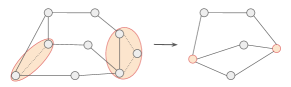
Figure 1: Graph reduction. Nodes connected by $\operatorname{\mathcal{E}}_{s}$ are collapsed into one node. The dash lines denote edges in $\operatorname{\mathcal{E}}_{s}$; the solid lines denote the edges in $\operatorname{\mathcal{E}}$.

The graph reduction step described above only makes sense when not all lines are switchable because otherwise, it results in a graph with a single node. For OTS scenarios where all lines are switchable, one can either skip the graph reduction step, or pre-select a set of lines that should remain non-switchable.

V-2 Graph partitioning

Our next step is to find an edge cut set $\operatorname{\mathcal{E}}_{c}$ of the graph $\operatorname{\mathcal{G}}_{r}$. In order to minimally affect the optimal value $p^{\operatorname{opt}}$, the graph partitioning is based on the optimal dual variables of (P3). The optimum dual variables measure how the optimal value $p^{\operatorname{opt}}_{3}$ of (P3) changes with respect to the corresponding constraint. Formally, by taking the derivative of the Lagrangian of (P3), we have the following for $i\in\operatorname{\mathcal{N}}\setminus\operatorname{\mathcal{N}}_{s}$,

$$\underline{\lambda}_{i}^{\operatorname{opt}_{3}}=\frac{\partial p^{\operatorname{opt}}_{3}}{\partial\underline{P}_{i}},\;\overline{\lambda}_{i}^{\operatorname{opt}_{3}}=\frac{\partial p^{\operatorname{opt}}_{3}}{\partial\overline{P}_{i}},\;\underline{\gamma}_{i}^{\operatorname{opt}_{3}}=\frac{\partial p^{\operatorname{opt}}_{3}}{\partial\underline{Q}_{i}},\;\overline{\gamma}_{i}^{\operatorname{opt}_{3}}=\frac{\partial p^{\operatorname{opt}}_{3}}{\partial\overline{Q}_{i}},$$

and for $i\in\operatorname{\mathcal{V}}$,

$$\underline{\lambda}_{i}^{\operatorname{opt}_{3}}=\sum_{k\in\operatorname{\mathcal{N}}_{s,i}}\frac{\partial p^{\operatorname{opt}}_{3}}{\partial\underline{P}_{k}},\;\overline{\lambda}_{i}^{\operatorname{opt}_{3}}=\sum_{k\in\operatorname{\mathcal{N}}_{s,i}}\frac{\partial p^{\operatorname{opt}}_{3}}{\partial\overline{P}_{k}},$$

$$\underline{\gamma}_{i}^{\operatorname{opt}_{3}}=\sum_{k\in\operatorname{\mathcal{N}}_{s,i}}\frac{\partial p^{\operatorname{opt}}_{3}}{\partial\underline{Q}_{k}},\;\overline{\gamma}_{i}^{\operatorname{opt}_{3}}=\sum_{k\in\operatorname{\mathcal{N}}_{s,i}}\frac{\partial p^{\operatorname{opt}}_{3}}{\partial\overline{Q}_{k}},$$

With this interpretation, we define edge weights as follows

$$A(i,k)=\begin{cases}\underset{l\in\{i,k\}}{\sum}\overline{\lambda}_{l}^{\operatorname{opt}_{3}}+\underline{\lambda}_{l}^{\operatorname{opt}_{3}}+\overline{\gamma}_{l}^{\operatorname{opt}_{3}}+\underline{\gamma}_{l}^{\operatorname{opt}_{3}},&\{i,k\}\in\operatorname{\mathcal{E}}_{r},\\ 0,&\text{otherwise}.\end{cases}$$

Given the adjacency matrix $A$, we do an $n$-optimal partition on $\operatorname{\mathcal{G}}_{r}$, which gives $\operatorname{\mathcal{G}}_{r}[\operatorname{\mathcal{V}}^{0}_{1}],\cdots,\operatorname{\mathcal{G}}_{r}[\operatorname{\mathcal{V}}^{0}_{n}]$ with $\cup_{i=1}^{n}\operatorname{\mathcal{V}}^{0}_{i}=(\operatorname{\mathcal{N}}\setminus\operatorname{\mathcal{N}}_{s})\cup\operatorname{\mathcal{V}}$. Since all the removed edges are in $\operatorname{\mathcal{E}}$, we can use the same cut for the partition of $\operatorname{\mathcal{G}}$: $\operatorname{\mathcal{G}}[\operatorname{\mathcal{V}}_{1}],\cdots,\operatorname{\mathcal{G}}[\operatorname{\mathcal{V}}_{n}]$ with $\cup_{i=1}^{n}\operatorname{\mathcal{V}}_{i}=\operatorname{\mathcal{N}}$. Such partition ensures $\operatorname{\mathcal{E}}_{c}\cap\operatorname{\mathcal{E}}_{s}=\emptyset$. The intuition is that the cut minimally perturbs $p^{\operatorname{opt}}$ because it select edges with minimal weight for the weighted graph $(\operatorname{\mathcal{G}},A)$.

Finding the optimal cut set is NP-hard. There are algorithms [29, 30] that can approximate it in a few seconds for graphs of the order of a thousand nodes. However, they do not guarantee that the resulting subgraphs are connected. To ensure this property, we resort to spectral graph partitioning.

Theorem V.1.

(Fiedler’s theorem of connectivity of spectral graph partitions). The two subgraphs resulting from spectral graph partitioning on a connected graph are also connected.

The proof is available in [31, Corollary 2.9]. To derive a $n$-partition, one can implement spectral graph partitioning recursively $n$ times. Since we aim for subgraphs with similar size, each iteration applies spectral graph partitioning on the subgraph with the largest number of nodes. The most computationally expensive step in this process is the eigenvector computation, which only takes linear time, or $\mathcal{O}(n)$. This low complexity is reflected on the negligible computational time in our simulations. Even though this recursive spectral partitioning does not in general lead to an $n$-optimal partition, we can characterize a lower bound for the sum of weights for each iteration $l$ of the recursive partitioning by

$$\frac{1}{2}C_{\operatorname{opt},l}^{2}\leq\sum_{\{i,k\}\in\operatorname{\mathcal{E}}_{c,l}}A(i,k),$$ (23)

where $C_{\operatorname{opt},l}$ is the optimal value for $2$-optimal partitioning and $\operatorname{\mathcal{E}}_{c,l}$ is the edge cut set in iteration $l$ (without loss of generality, we have assume $A$ is normalized). Inequality (23) follows directly from Cheeger inequalities [32] and the Courant-Fischer Theorem [33].

V-3 Integer optimization on subgraphs

Given a $n$-partition $\{\operatorname{\mathcal{G}}[\operatorname{\mathcal{V}}_{l}]\}_{l=1}^{n}$, we define an optimization problem associated with each subgraph. This problem is a variant of (P2) that is convenient for the reconstruction of the solution of (P2) over the original $\operatorname{\mathcal{G}}$. For subgraph $l$, let $\operatorname{\mathcal{E}}_{l}$ be its set of edges, $W_{l}\in\operatorname{\mathbb{S}}_{+}^{|\operatorname{\mathcal{V}}_{l}|}$ the decision variable, $\hat{\operatorname{\mathcal{E}}}_{s,l}$ the set of switchable lines, and $\operatorname{\mathcal{B}}_{l}$ the set of nodes in $\operatorname{\mathcal{V}}_{l}$ that connects to at least one node of another subgraph. Each subgraph $l$ solves

$$\textbf{(P4)}\min_{\begin{subarray}{c}W_{l}\succeq 0,\alpha_{ik}\in\{0,1\},\;\forall\{i,k\}\in\hat{\operatorname{\mathcal{E}}}_{s,i}\end{subarray}}\sum\nolimits_{i\in\operatorname{\mathcal{N}}_{G}\cap\operatorname{\mathcal{V}}_{l}}\Big{(}c_{i2}P_{i}^{2}+c_{i1}P_{i}\Big{)},$$

subject to

$$\underline{P}_{i}\leq P_{i}\leq\overline{P}_{i},\quad\underline{Q}_{i}\leq Q_{i}\leq\overline{Q}_{i},\;\forall i\in\operatorname{\mathcal{V}}_{l},$$

$$\underline{V}_{i}^{2}\leq\operatorname{\bf Tr}\{M_{i}W_{l}\}\leq\overline{V}_{i}^{2},\;\forall i\in\operatorname{\mathcal{V}}_{l},$$

$$\operatorname{\bf Tr}\{M_{ik}W_{l}\}\leq\overline{V}_{ik},\;\forall\{i,k\}\in\operatorname{\mathcal{E}}_{l}.$$

$$\text{For all }i\in\operatorname{\mathcal{V}}_{l}\setminus\operatorname{\mathcal{B}}_{l},$$

$$P_{i}=\operatorname{\bf Tr}\{Y_{i}W_{l}\}+P_{D_{i}}+\sum\nolimits_{k,\{i,k\}\in\operatorname{\mathcal{E}}_{s,i}}\alpha_{ik}\operatorname{\bf Tr}\{Y_{ik}W_{l,ik}\},$$

$$Q_{i}=\operatorname{\bf Tr}\{\overline{Y}_{i}W_{l}\}+Q_{D_{i}}+\sum\nolimits_{k,\{i,k\}\in\operatorname{\mathcal{E}}_{s,i}}\alpha_{ik}\operatorname{\bf Tr}\{\overline{Y}_{ik}W_{l,ik}\}.$$

$$\text{For all }i\in\operatorname{\mathcal{B}}_{l},$$

$$P_{i}=\operatorname{\bf Tr}\{Y_{i}W_{l}\}+P_{D_{i}}+\operatorname{\mathcal{P}}_{l,i}+\sum_{k,\{i,k\}\in\operatorname{\mathcal{E}}_{s,i}}\alpha_{ik}\operatorname{\bf Tr}\{Y_{ik}W_{l,ik}\},$$

$$Q_{i}=\operatorname{\bf Tr}\{\overline{Y}_{i}W_{l}\}+Q_{D_{i}}+\operatorname{\mathcal{Q}}_{l,i}+\sum_{k,\{i,k\}\in\operatorname{\mathcal{E}}_{s,i}}\alpha_{ik}\operatorname{\bf Tr}\{\overline{Y}_{ik}W_{l,ik}\},$$

where $\operatorname{\mathcal{P}}_{l,i}=\sum_{k\in\operatorname{\mathcal{N}}\setminus\operatorname{\mathcal{V}}_{l},\{i,k\}\in\operatorname{\mathcal{E}}}P_{ik}^{\operatorname{opt}_{3}}$ sums the active power flow from the solution of (P3), $\operatorname{\mathcal{Q}}_{l,i}$ is defined similarly, and with a slight abuse of notation, all $M_{i}$, $M_{ik}$, $Y_{i}$, $\overline{Y}_{i}$, $Y_{ik}$ take proper dimensions matching $W_{l}$. Notice that (P4) is still NP-hard due to $\alpha_{ik}$, but the number of switches $|\operatorname{\mathcal{E}}_{s,i}|$ in each partition is less than $|\operatorname{\mathcal{E}}_{s}|$, and decreases with $n$. The addition of $\operatorname{\mathcal{P}}_{l,i}$ and $\operatorname{\mathcal{Q}}_{l,i}$ in (P4) accounts for the coupling between $\operatorname{\mathcal{G}}[\operatorname{\mathcal{V}}_{l}]$ and the other subgraphs. For each subgraph, these terms are constant and do not provide an exact approximation of the power exchanged between the subgraphs – since they do not take into account the dependency of the terminal voltage on the solutions determined on the other subgraphs. Therefore, putting together the solutions obtained for each subgraph may not result in a feasible solution of (P2), but rather a solution to (P2) with a perturbation on (6c). We address this next.

V-4 Full SDP optimization with fixed topology

In the last step, we define the candidate optimal switch $\alpha_{p}^{\operatorname{opt}}\in\{0,1\}^{|\operatorname{\mathcal{E}}_{s}|}$ from the solutions of (P4) obtained in the previous step. With this in place, we solve (P1)-$\alpha^{\operatorname{opt}}_{p}$ to obtain the candidate optimal solution $W^{\operatorname{opt}}_{p}$ and output $(\alpha^{\operatorname{opt}}_{p},W^{\operatorname{opt}}_{p})$ as the reconstructed solution of (P2).

VI Simulation Studies

In this section we illustrate the performance of the virtual-voltage approximation and the partition-based OTS algorithm on standard IEEE test systems. All simulations are done on a desktop with 3.5GHz CPU and 16GB RAM, using MATLAB and its CVX toolbox [34] to solve the convex optimization problems. In all our tables except the last row in Table III, “lower bound” refers to the optimal value of (P3) and “upper bound” refers to the optimal value of (P1)-$\alpha$, where $\alpha$ is determined by the corresponding method.

VI-A Comparison with McCormick Relaxation

We implement the virtual-voltage approximation and compare its performance against the solution obtained from (P2) with the McCormick approximation (cf. Remark IV.7). For the latter, we use two different estimates on the upper bounds of the line power flows. In one case, we use the conservative bounds $\overline{P}_{ik}=-\underline{P}_{ik}=5$(p.u.) and $\overline{Q}_{ik}=-\underline{Q}_{ik}=5$(p.u.) for all $\{i,k\}\in\hat{\operatorname{\mathcal{E}}}_{s}$. These bounds come from the heuristic estimation on the largest line active/reactive power flow. In the other case, we set the tighter bounds $\overline{P}_{ik}=-\underline{P}_{ik}=1$(p.u.) and $\overline{Q}_{ik}=-\underline{Q}_{ik}=0.5$(p.u.) for all $\{i,k\}\in\hat{\operatorname{\mathcal{E}}}_{s}$, based on our knowledge of the solution of the IEEE test nominal case. We include an additional cost function on the line power losses to promote optimal solutions with some edges disconnected. For each test case, a set of switchable lines are selected by the following policy: given a design parameter $p\in\operatorname{\mathbb{N}}$, we rank all lines by the norm of their admittance in ascending order and select the first $p$ as the set of switchable lines. The rationale for this selection is that each line with small admittance places a small correlation between its terminal nodes and, as a result, they are more likely to be disconnected. The selection of $p$ is based on the size of the network.

		IEEE 30	IEEE 39	IEEE 57	IEEE 89	IEEE 118	IEEE 300
	$\#$ of switches	5	5	5	30	40	40
Virtual-voltage approximation	lower bound	1265 (1)	135003 (1)	50912 (1)	179325 (1)	151594 (3)	1086369 (1)
	upper bound	1270 (1)	135303 (1)	52267 (2)	188896 (1)	152707 (1)	1096117 (1)
McCormick relaxation w/ $5$(p.u.) bounds	lower bound	1046 (1)	133591 (4)	50209 (1)	177643 (1)	146466 (1)	1054130 (2)
	upper bound	4654 (3)	135660 (1)	52267 (2)	230355 (1)	153477 (1)	NaN
McCormick relaxation w/ $1$(p.u.) bounds	lower bound	1046 (1)	133591 (1)	50209 (1)	NaN	147919 (1)	NaN
	upper bound	NaN	135303 (1)	67667 (2)	NaN	152484 (1)	NaN

TABLE I: Performance of the virtual-voltage and the McCormick approximation. The integer value in parentheses is the rank of the SDP solutions. “NaN” means that CVX cannot find a feasible solution (even though the problem may still be feasible, see [35] for details).

The virtual-voltage approach yields discrete variables close to $\{0,1\}$ for all the test cases and, in contrast, the McCormick relaxation has most of them around $0.5$. Table I shows the values obtained by both approximations, and confirms that the virtual-voltage approach gives better solutions than the McCormick relaxation. It is worthwhile to note that every virtual voltage matrix $U$ has its condition number comfortably more than 1000 for all the test cases. The smallest condition number is 1492. This validates the statements of Lemma IV.1 and Remark IV.2 for a physically meaningful virtual voltage.

In both the McCormick relaxation and virtual-voltage methods, the number of decision variables grows linearly with respect to $p$. Though $p$ is relatively small compared to the dimension of $W$ and is not the main factor for optimization complexity, we observe in Table II that for a given $p$, the McCormick relaxation returns a solution noticeably faster than the virtual-voltage method. The reason is that the McCormick relaxation does not introduce LMIs for the switchable lines. In this regard, the virtual-voltage approach trades time complexity for better-quality solutions.

		IEEE 30	IEEE 39	IEEE 57	IEEE 89	IEEE 118	IEEE 300
	$\#$ of switches	5	5	5	30	40	300
Virtual-voltage approximation	lower bound	7.78	9.55	18.72	59.01	149.37	2668
	upper bound	5.52	6.71	12.63	39.05	88.55	2356
McC. relaxation w/ $5$(p.u.) bounds	lower bound	4.93	7.69	12.92	57.19	99.19	2394
	upper bound	5.1	5.8	12.62	44.48	88.28	2250
McC. relaxation w/ $1$(p.u.) bounds	lower bound	6.24	5.8	13.34	94.51	104.18	2338
	upper bound	5.82	6.61	9.87	42.25	87.88	2311

TABLE II: Comparison of the computational time between McCormick and virtual-voltage approximations.

VI-B Comparison with BARON

We compare the virtual-voltage approximation with the general purpose mixed-integer nonlinear programming solver BARON [36] in several small-scale IEEE examples. With the default settings and maximal computational time at 1000 seconds, BARON does not always return a feasible solution, see Table III.

		IEEE 30		IEEE 39		IEEE 57
$\#$ of switchable lines		5	10	1	5	1	5
Virtual-voltage approx.	lower bound	1265	1265	135295	135003	50997	50912
	upper bound	1269.9	1269.9	135303	135303	52267	52267
BARON	lower bound	$-2.2\cdot 10^{7}$	$-2.3\cdot 10^{7}$	$-2.7\cdot 10^{8}$	$-2.6\cdot 10^{8}$	$-6.8\cdot 10^{7}$	$-6.9\cdot 10^{7}$
	upper bound	1269.9	1269.9	135303	$3.4\cdot 10^{8}$	$7.6\cdot 10^{8}$	$7.6\cdot 10^{8}$

TABLE III: Comparison between solutions of BARON and virtual-voltage approximation. We pre-select 5 switchable lines for all the test cases.

We observe that BARON gives a feasible solution only when it finds one in the preprocessing stage, which happens for the IEEE 30 bus test case and the IEEE 39 bus test case with one switchable line. The branch-and-bound process made in BARON only slowly increases the lower bound, and barely refines the upper bound given in the preprocessing stage. On top of discrete binary variables for switching, OTS involves nonlinearities coming from bilinear products. All these factors can prevent general purpose solvers such as BARON from finding the optimal solution efficiently. On the other hand, the virtual-voltage approximation is built on provably accurate SDP relaxations of OPF and makes use of the specific structure of the OTS problem. Table III clearly shows the difference in performance between both methods.

VI-C Partition-based OTS algorithm

We examine here the performance of the partition-based algorithm. Table IV shows the result of implementing on the IEEE 118 and IEEE 300 bus test cases the following methods: (i) the virtual-voltage approximation with 40 switchable lines; and (ii) the partition-based OTS algorithm with $40$ switchable lines; and (iii) the virtual-voltage approximation with all the lines switchable. For the case with 40 switchable lines, one can see that the partition-based OTS algorithm refines the virtual-voltage approximation. The solutions obtained by the virtual-voltage approximation and the partition-based OTS algorithm with 40 switchable lines are both close to the lower bound. In addition, SDP returns a rank-1 solution for every case with 40 switchable lines. We quantify their accuracy by upper bounding the percentage error with the true optimal solution using $(p^{\operatorname{opt}}_{1}-p^{\operatorname{opt}}_{3,\text{all}})/{p^{\operatorname{opt}}_{3,\text{all}}}\cdot 100\%$.

We simulate case (iii) where all the lines are switchable to compare the results with the QC relaxation method [15]. The QC relaxation method takes 10 hours to solve the OTS problem for both IEEE 118 and 300 bus test cases employing servers with 4334 CPUs and 64GB memory. The QC relaxation method converges to a near optimum with around $1\%$ error for the IEEE 118 test case, while it is unable to provide a feasible solution for the IEEE 300 bus case. In contrast, solving (P3) with all lines switchable takes significantly less time for both cases (around 2min30sec and 1h30min, respectively) as shown in Table IV. Though we only retrieve a rank-2 solution from (P3) for IEEE 118 bus case, the condition number of the decision variable $W$ is larger than 250, which translates to an error (or violation of constraints) less than $1\%$. Therefore, the virtual-voltage approximation leads to a solution of a similar quality as QC. The reason of not retrieving a rank-1 solution with the virtual-voltage approximation is that it provides high-rank solutions when the $U$ matrix is introduced on every line (this is one of the reasons for pre-selecting a subset of lines).

		Optimal values		Bound on errors		Computation times (sec)
		IEEE 118	IEEE 300	IEEE 118	IEEE 300	IEEE 118	IEEE 300
Virtual-voltage approximation w/ all lines switchable	lower bound	150791 ($\overline{10}$)	1090397 ($\overline{10}$)	$0.36\%$	N/A	142.57	4859.62
	upper bound	151340 (2)	NaN
Virtual-voltage approximation w/ 40 switchable lines	lower bound	151594 (1)	1086369 (1)	$1.27\%$	$0.52\%$	149.37	5023.90
	upper bound	152707 (1)	1096117 (1)
Partition-based OTS w/ 40 switchable lines		152505 (1)	1092967 (1)	$1.14\%$	$0.24\%$	173	5055.88

TABLE IV: Performance of the virtual-voltage approximation and the partition-based OTS algorithm on the IEEE 118 and IEEE 300 bus test cases. $(\overline{10})$ indicates that the rank of the decision variable is larger than 10.

VI-D OTS with Security Constraints

We also validate the virtual-voltage approximation method on OTS with security constraints. We simulate both IEEE 118 and 300 bus test systems with one contingency scenario and 40 pre-selected switchable lines. Table V shows the results for the IEEE 118 bus test system with security constraint on line $\{106,107\}$. The combined computational time in computing the lower and upper bounds raises to 834 (395+438) seconds, which is longer than the one without security constraint (149.37 seconds in Table IV). For the IEEE 300 bus test case, CVX cannot find a feasible solution even when we increase the maximal iterations to $600$ (the default is $100$ iterations), which took around 3.7 hours. The drastic increase on the computational time limits the applicability of the SDP-based approach to OTS with security constraints.

	Optimal Value	Time (sec)
lower bound	156896 (5)	396
upper bound	158660 (1)	438

TABLE V: Performance of the virtual-voltage approximation for OTS with security constraint on line $\{106,107\}$.

VII Conclusions

We have considered OTS problems with security constraints. For these scenarios, the standard SDP relaxation of the problem remains non-convex because of the presence of bilinear terms and the discrete variables. We have proposed an approximation based on the introduction of virtual-voltages to convexify the bilinear terms. We have also characterized several of its properties regarding physical interpretation and lower and upper bounds on the optimal value of the original problem. To handle the presence of the discrete variables, we have built on the virtual-voltage approximation to propose a graph partition-based algorithm that significantly reduces the computational complexity of solving the original problem. The high degree of accuracy and the reduction in computational complexity observed in simulations makes the proposed algorithms promising for OTS applications. Future work will incorporate other types of discrete controls, and investigate distributed methods for general mixed-integer OPF problems.

References

- [1] C.-Y. Chang, S. Martínez, and J. Cortés, “Convex relaxation for mixed-integer optimal power flow problems,” in Allerton Conf. on Communications, Control and Computing, Monticello, IL, 2017, pp. 307–314.
- [2] J. Momoh, M. El-Hawary, and R. Adapa, “A review of selected optimal power flow literature to 1993. Part I: Nonlinear and quadratic programming approaches,” IEEE Transactions on Power Systems, vol. 14, no. 1, pp. 96–104, 1999.
- [3] S. Frank, I. Steponavice, and S. Rebennack, “Optimal power flow: a bibliographic survey I,” Energy Systems, vol. 3, no. 3, pp. 221–258, 2012.
- [4] H. Abdi, S. D. Beigvand, and M. L. Scala, “A review of optimal power flow studies applied to smart grids and microgrids,” Renewable and Sustainable Energy Reviews, vol. 71, pp. 742–766, 2017.
- [5] M. R. AlRashidi and M. E. El-Hawary, “A survey of particle swarm optimization applications in electric power systems,” IEEE Transactions on Evolutionary Computation, vol. 13, no. 4, pp. 913–918, 2009.
- [6] P. E. O. Yumbla, J. M. Ramirez, and C. A. Coello, “Optimal power flow subject to security constraints solved with a particle swarm optimizer,” IEEE Transactions on Power Systems, vol. 23, no. 1, pp. 33–40, 2008.
- [7] A. G. Bakirtzis, P. N. Biskas, C. E. Zoumas, and V. Petridis, “Optimal power flow by enhanced genetic algorithm,” IEEE Transactions on Power Systems, vol. 17, no. 2, pp. 229–236, 2002.
- [8] K. W. Hedman, S. S. Oren, and R. P. O’Neill, “A review of transmission switching and network topology optimization,” in IEEE Power and Energy Society General Meeting, Detroit, MI, 2011, electronic proceedings.
- [9] J. G. Rolim and L. J. B. Machado, “A study of the use of corrective switching in transmission systems,” IEEE Transactions on Power Systems, vol. 14, no. 1, pp. 336–341, 1999.
- [10] J. D. Fuller, R. Ramasra, and A. Cha, “Fast heuristics for transmission-line switching,” IEEE Transactions on Power Systems, vol. 27, no. 3, pp. 1377–1386, 2012.
- [11] P. A. Ruiz, J. M. Foster, A. Rudkevich, and M. C. Caramanis, “Tractable transmission topology control using sensitivity analysis,” IEEE Transactions on Power Systems, vol. 27, no. 3, pp. 1550–1559, 2012.
- [12] S. Fattahi, J. Lavaei, and A. Atamtürk, “A bound strengthening method for optimal transmission switching in power systems,” arXiv preprint arXiv:1711.10428, 2017.
- [13] T. Potluri and K. W. Hedman, “Impacts of topology control on the ACOPF,” in IEEE Power and Energy Society General Meeting, San Diego, CA, 2012, electronic proceedings.
- [14] M. Soroush and J. D. Fuller, “Accuracies of optimal transmission switching heuristics based on DCOPF and ACOPF,” IEEE Transactions on Power Systems, vol. 29, no. 2, pp. 924–932, 2014.
- [15] H. Hijazi, C. Coffrin, and P. Van Hentenryck, “Convex quadratic relaxations for mixed-integer nonlinear programs in power systems,” Mathematical Programming Computation, vol. 9, no. 3, pp. 321–367, 2017.
- [16] J. Mareček, M. Mevissen, and J. C. Villumsen, “MINLP in transmission expansion planning,” in Power Systems Computation Conference, Genoa, Italy, 2016, electronic proceedings.
- [17] E. Briglia, S. Alaggia, and F. Paganini, “Distribution network management based on optimal power flow: Integration of discrete decision variables,” in Annual Conference on Information Systems and Sciences, Baltimore, MD, 2017, electronic proceedings.
- [18] G. P. McCormick, “Computability of global solutions to factorable nonconvex programs: Part I – convex underestimating problems,” Mathematical programming, vol. 10, no. 1, pp. 147–175, 1976.
- [19] F. Bullo, J. Cortés, and S. Martínez, Distributed Control of Robotic Networks, ser. Applied Mathematics Series. Princeton University Press, 2009, electronically available at http://coordinationbook.info.
- [20] J. Lavaei and S. H. Low, “Zero duality gap in optimal power flow problem,” IEEE Transactions on Power Systems, vol. 27, no. 1, pp. 92–107, 2012.
- [21] R. Madani, M. Ashraphijuo, and J. Lavaei, “Promises of conic relaxation for contingency-constrained optimal power flow problem,” IEEE Transactions on Power Systems, vol. 31, no. 2, pp. 1297–1307, 2016.
- [22] R. A. Jabr, R. Singh, and B. C. Pal, “Minimum loss network reconfiguration using mixed-integer convex programming,” IEEE Transactions on Power Systems, vol. 27, no. 2, pp. 1106–1115, 2012.
- [23] P. A. Ruiz, A. Rudkevich, M. C. Caramanis, E. Goldis, E. Ntakou, and C. R. Philbrick, “Reduced MIP formulation for transmission topology control,” in Allerton Conf. on Communications, Control and Computing, Monticello, IL, 2012, pp. 1073–1079.
- [24] A. J. Wood and B. F. Wollenberg, Power generation, operation, and control. John Wiley & Sons, 2012.
- [25] E. B. Fisher, R. P. O’Neill, and M. C. Ferris, “Optimal transmission switching,” IEEE Transactions on Power Systems, vol. 23, no. 3, pp. 1346–1355, 2008.
- [26] K. W. Hedman, R. P. O’Neill, E. B. Fisher, and S. S. Oren, “Optimal transmission switching with contingency analysis,” IEEE Transactions on Power Systems, vol. 24, no. 3, pp. 1577–1586, 2009.
- [27] M. Khanabadi, H. Ghasemi, and M. Doostizadeh, “Optimal transmission switching considering voltage security and N-1 contingency analysis,” IEEE Transactions on Power Systems, vol. 28, no. 1, pp. 542–550, 2013.
- [28] I. E. Grossmann, “Review of nonlinear mixed-integer and disjunctive programming techniques,” Optimization and Engineering, vol. 3, no. 3, pp. 227–252, 2002.
- [29] J. P. Hespanha, “An efficient Matlab algorithm for graph partitioning,” University of California, Santa Barbara, Tech. Rep., 2004.
- [30] A. Abou-Rjeili and G. Karypis, “Multilevel algorithms for partitioning power-law graphs,” in International Parallel and Distributed Processing Symposium (IPDPS), Rhodes Island, Greece, 2006, electronic proceedings.
- [31] M. Fiedler, “A property of eigenvectors of nonnegative symmetric matrices and its application to graph theory,” Czechoslovak Mathematical Journal, vol. 25, no. 4, pp. 619–633, 1975.
- [32] F. Chung, “Four Cheeger-type inequalities for graph partitioning algorithms,” Proceedings of ICCM, pp. 751–772, 2007.
- [33] B. Mohar, Y. Alavi, G. Chartrand, and O. Oellermann, “The Laplacian spectrum of graphs,” Graph theory, combinatorics, and applications, vol. 2, no. 871-898, p. 12, 1991.
- [34] M. Grant and S. Boyd, “CVX: Matlab software for disciplined convex programming, version 2.1,” Mar. 2014, available at http://cvxr.com/cvx.
- [35] M. Grant, S. Boyd, and Y. Ye, “CVX users’ guide,” 2009.
- [36] The Optimization Firm, “BARON,” https://minlp.com/baron.