Optimality and resonances in a class of compact finite difference schemes of high order

Abstract

In this paper, we revisit the old problem of compact finite difference approximations of the homogeneous Dirichlet problem in dimension $1$. We design a large and natural set of schemes of arbitrary high order, and we equip this set with an algebraic structure. We give some general criteria of convergence and we apply them to obtain two new results. On the one hand, we use Padé approximant theory to construct, for each given order of consistency, the most efficient schemes and we prove their convergence. On the other hand, we use diophantine approximation theory to prove that almost all of these schemes are convergent at the same rate as the consistency order, up to some logarithmic correction.

1 Introduction

Many decades ago, compact finite differences methods were widely studied. Nowadays, we can find a huge literature about these methods that are widely applied and used for the approximation of partial differential equations (see, for example, [3] or [10]). In particular, we can find a lot of examples of accurate schemes for elliptic problems and many classical mathematical arguments are proposed to prove their convergence (monotonicity, energy, green functions, …). However, it seems that there is not general and algebraic study of compact finite difference schemes for elliptic problems, equivalent to what we can find, for example, for the Runge Kutta methods applied to Cauchy problems (general stability criteria, algebraic order conditions using Hopf algebras and trees as we can see in [6] or [5]).

As the field of elliptic problems is clearly too wide, we propose, in this paper, a general study of a large and natural class of compact finite difference schemes of high order for the homogeneous Dirichlet problem in dimension $1$. In this context, a compact finite difference scheme is a linear system of the form

$$\mathbf{D}_{N}\mathbf{u}^{N}=\mathbf{S}_{N}\mathbf{f}^{N,ex},$$

where $\mathbf{f}^{N,ex}$ is a discretization of the source term on a grid of stepsize $h=(N+1)^{-1}$, $\mathbf{D}_{N}$ and $\mathbf{S}_{N}$ are matrices and $\mathbf{u}^{N}$ is the approximation of the solution of the Dirichlet problem.

To study their convergence (i.e. the approximation of the exact solution by $\mathbf{u}^{N}$), we first introduce some specific and rigorous notions of consistency and stability taking into account the boundary conditions. Then, we describe precisely the class of schemes that we consider, namely when the matrix $\mathbf{D}_{N}$ is a polynomial in the usual discrete second derivative matrix $\mathbf{A}_{N}$ defined by

$$\mathbf{A}_{N}=\left(\begin{matrix}2&-1\\ -1&2&-1\\ &\ddots&\ddots&\ddots\\ &&-1&2&-1\\ &&&-1&2\end{matrix}\right)\in\mathscr{L}(\mathbb{C}^{N}).$$ (1)

This choice is made for two reasons. First it allows for a relatively simple stability analysis, and second it is in fact not so restrictive. Indeed, if we take a symmetric finite difference formula $d=(d_{j})_{j\in\mathbb{Z}}$ that approximates the second derivative, i.e. for all smooth function $u$,

$$\sum_{j\in\mathbb{Z}}d_{j}u(hj)\simeq-h^{2}u^{\prime\prime}(0),$$

then we get, from a convolution formula and for some specific and natural choice of the coefficients near the boundary, a matrix $\mathbf{D}_{N}$ that is a polynomial in $\mathbf{A}_{N}$.

In this paper, we give some general criterion of convergence for this family of schemes. Moreover, we address the following two questions:

• Are these schemes stable in general  ?

• Amongst these schemes, what are the most efficient and are they stable?

We will precise the two ambiguous terms general and efficient by introducing, on one hand, a Lebesgue measure on the set of schemes, and on the other hand, an optimization problem defining efficiency. The first main result of this paper will be to prove that almost all schemes are convergent at the same rate as its consistency order, up to some logarithmic correction. It is based on a careful analysis of small denominators appearing in the stability conditions, linked with diophantine approximation theory. The second main result of this paper is the design and construction of the most efficient schemes in the class considered, which turn to be stable, this latter property requiring the use of Padé approximant theory to be proved.

2 Formalism and main results

The goal of this section is to present the two main results of this paper. To this aim, we first define rigorously compact finite difference schemes for the homogeneous Dirichlet problem in dimension $1$. Then, we recall the usual concept of convergence, consistency and stability for these schemes. And finally, we define the particular set of schemes that we consider.

2.1 Context

We consider the homogeneous Dirichlet problem in dimension $1$, namely:

For a given $f:\mathbb{R}\to\mathbb{C}$, find $u:[0,1]\to\mathbb{C}$ such that

$$\left\{\begin{array}[]{lll}-u^{\prime\prime}(x)=f(x),\ \forall x\in]0,1[,\\ u(0)=u(1)=0.\end{array}\right.$$ (2)

To design finite difference schemes, we will consider regular grids on $\mathbb{R}$. More precisely, we choose $N\in\mathbb{N}^{*}$ to be the number of grid points into $]0,1[$ (the number of unknowns) and we define $h$ as the stepsize of the grid. As a consequence, $h$ and $N$ are linked by the relation

$$h=\frac{1}{N+1}.$$

Let $x_{j}^{N}=jh$, $j\in\mathbb{Z}$ denote the grid points, see Figure 1.

Figure 1: Regular grid with $N$ points into $]0,1[$.

In this context, a finite difference scheme is a couple of sequences of matrices $((\mathbf{D}_{N})_{N\in\mathbb{N}^{*}},(\mathbf{S}_{N})_{N\in\mathbb{N}^{*}})$ such that $\mathbf{D}_{N}\in\mathscr{L}(\mathbb{C}^{N})$ is a square matrix of size $N$ and $\mathbf{S}_{N}\in\mathscr{L}(\mathbb{C}^{\mathbb{Z}};\mathbb{C}^{N})$ is a rectangle matrix with $N$ rows and a finite number of columns.

If $\mathbf{D}_{N}$ is invertible for all $N$, such a scheme leads to an approximation of the solution $u$ of the Dirichlet problem (2). More precisely, we define $\mathbf{f}^{N,ex}$ and $\mathbf{u}^{N,ex}$ as the vectors of the values of $f$ and $u$ on the grid:

$$\mathbf{f}^{N,ex}=(f(x_{j}^{N}))_{j\in\mathbb{Z}}\in\mathbb{C}^{\mathbb{Z}}\textrm{ and }\mathbf{u}^{N,ex}=(u(x_{j}^{N}))_{j\in\llbracket 1,N\rrbracket}\in\mathbb{C}^{N}.$$ (3)

Then, the scheme gives an approximation $\mathbf{u}^{N}$ of $\mathbf{u}^{N,ex}$ through the solution of the linear system

$$\mathbf{D}_{N}\mathbf{u}^{N}=h^{2}\mathbf{S}_{N}\mathbf{f}^{N,ex}.$$ (4)

It may seem unusual to use the values of $f$ outside $[0,1]$ but it is just a way to have more symmetric formulas. In practice, as we will explain in the subsection 2.3, we only use a finite number of values of $f$ outside $[0,1]$ independent of $N$ and at a distance of order $h$ of $[0,1]$. Consequently, as we will assume that $f$ is a regular function, these values could be extrapolated from those of $f$ in $[0,1]$ with some Newton series.

To estimate the accuracy of a scheme, we define a notion of rate of convergence and of order of convergence. Let $(\epsilon_{N})_{N\in\mathbb{N}^{*}}$ be a sequence of positive numbers that tends to $0$, as $N$ goes to infinity. Then, a scheme $((\mathbf{D}_{N})_{N\in\mathbb{N}^{*}},(\mathbf{S}_{N})_{N\in\mathbb{N}^{*}})$ is said to be convergent at the rate $(\epsilon_{N})_{N\in\mathbb{N}^{*}}$, if $\mathbf{D}_{N}$ is invertible for all $N\in\mathbb{N}^{*}$ and if for all $f\in C^{\infty}(\mathbb{R})$ there exists a constant $c>0$ such that for all $N\in\mathbb{N}^{*}$,

$$\sup_{j=1,\dots,N}|\mathbf{u}^{N}_{j}-\mathbf{u}^{N,ex}_{j}|=:\|\mathbf{u}^{N,ex}-\mathbf{u}^{N}\|_{\infty}\leq c\epsilon_{N}.$$ (5)

Furthermore, if $n$ is a positive integer and $\epsilon_{N}=h^{n}$, then a scheme that is convergent at the rate $(\epsilon_{N})_{N\in\mathbb{N}^{*}}$ is said to be convergent of order $n$.

2.2 Notions of consistency and stability

In order to establish a convergence result of the form (5), we use introduce the notions of consistency and stability. Then, we give a Lax theorem to deduce the convergence from the consistency and the stability.

A scheme $((\mathbf{D}_{N}),(\mathbf{S}_{N}))$ is said to be consistent of order $n\in\mathbb{N}$, if for all $f\in C^{\infty}(\mathbb{R})$ there exists a constant $c>0$ such that for all $N\in\mathbb{N}^{*}$, the vectors $\mathbf{u}^{N,ex}$ and $\mathbf{f}^{N,ex}$, defined by (3), verify

$$\|\mathbf{D}_{N}\mathbf{u}^{N,ex}-h^{2}\mathbf{S}_{N}\mathbf{f}^{N,ex}\|_{\infty}\leq ch^{n+2}.$$ (6)

In the context of the Dirichlet problem, it is usual to relax this notion of consistency near the boundary (see [3]). A scheme $((\mathbf{D}_{N}),(\mathbf{S}_{N}))$ is said to be consistent of order $n\in\mathbb{N}$ in the center and of order $n-2$ at a distance $l\in\mathbb{N}$ of the boundary, if for all $f\in C^{\infty}(\mathbb{R})$ there exists a constant $c>0$ such that for all $N\in\mathbb{N}^{*}$, the vectors $\mathbf{u}^{N,ex}$ and $\mathbf{f}^{N,ex}$, defined by (3), verify for all $j=1,\dots,N$,

$$\left|\left(\mathbf{D}_{N}\mathbf{u}^{N,ex}\right)_{j}-h^{2}\left(\mathbf{S}_{N}\mathbf{f}^{N,ex}\right)_{j}\right|\leq\left\{\begin{array}[]{lll}ch^{n+2}&\textrm{ if }l<j<N+1-l,\\ ch^{n}&\textrm{ else.}\end{array}\right.$$ (7)

In this article, it is useful to distinguish some notions of stability. A scheme $((\mathbf{D}_{N}),(\mathbf{S}_{N}))$ or a sequence $\displaystyle(\mathbf{D}_{N})_{N\in\mathbb{N}^{*}}\in\prod_{N\in\mathbb{N}^{*}}\mathscr{L}(\mathbb{C}^{N})$ of matrices is said to be

• stable, if there exists a positive constant $c>0$ such that for all $N\in\mathbb{N}^{*}$, we have

  $$\forall\mathbf{v}\in\mathbb{C}^{N},\ c\|\mathbf{v}\|_{\infty}\leq h^{-2}\|\mathbf{D}_{N}\mathbf{v}\|_{\infty}.$$ (8)

• strongly stable, if for all $l\in\mathbb{N}$, there exists a positive constant $c>0$ such that for all $N\in\mathbb{N}^{*}$,

  $$\forall\mathbf{v}\in\mathbb{C}^{N},\ c\|\mathbf{v}\|_{\infty}\leq\sup_{j=1,\dots,N}\left\{\begin{array}[]{lll}h^{-2}\left(\mathbf{D}_{N}\mathbf{v}\right)_{j}&\textrm{ if }l<j<N+1-l,\\ \left(\mathbf{D}_{N}\mathbf{v}\right)_{j}&\textrm{ else.}\end{array}\right..$$ (9)

• stable relatively to a sequence $(\eta_{N})_{N\in\mathbb{N}^{*}}$ of positive numbers, if there exists a positive constant $c>0$ such that for all $N\in\mathbb{N}^{*}$, we have

  $$\forall\mathbf{v}\in\mathbb{C}^{N},\ c\|\mathbf{v}\|_{\infty}\leq\eta_{N}\|\mathbf{D}_{N}\mathbf{v}\|_{\infty}.$$ (10)

We remark that, if a scheme is strongly stable, then it is stable, and, if it is stable, then it is stable relatively to $\eta_{N}=(N+1)^{2}=h^{-2}$.

To establish convergence from consistency and stability, we give a Lax theorem.

Theorem 2.1.

Lax

• A scheme that is strongly stable (see (9)) and consistent of order $n\geq 1$ in the center and of order $n-2$ at a distance $l\in\mathbb{N}$ of the boundary (see (7)) is convergent of order $n$.

• Let $(\eta_{N})_{N\in\mathbb{N}^{*}}$ be a sequence of positive number and $n\in\mathbb{N}^{*}$ such that the sequence $(\eta_{N}h^{n+2})_{N\in\mathbb{N}^{*}}$ tends to zero as $N$ goes to infinity. Then a scheme that is stable relatively to the sequence $(\eta_{N})_{N\in\mathbb{N}^{*}}$ (10) and consistent of order $n$ (6) is convergent at the rate $\epsilon_{N}=\eta_{N}h^{n+2}$ (5).

Proof.

The invertibility of $\mathbf{D}_{N}$ follows from the stability estimate. To prove the convergence estimate, it is enough to apply the stability estimate to the error of consistency

$$\mathbf{D}_{N}\mathbf{v}=\mathbf{D}_{N}\left(\mathbf{u}^{N,ex}-\mathbf{u}^{N}\right)=\mathbf{D}_{N}\mathbf{u}^{N,ex}-h^{2}\mathbf{S}_{N}\mathbf{f}^{N,ex}.$$

∎

2.3 Expression of the schemes

Usually, to design a finite difference scheme $((\mathbf{D}_{N}),(\mathbf{S}_{N}))$, we need to introduce the notion of finite difference formulas. A finite difference formula is a sequence of complex numbers indexed by $\mathbb{Z}$ with finite support. We denote by $\mathbb{C}^{(\mathbb{Z})}$ their space. We say that a couple of finite difference formulas $(d,s)\in\left(\mathbb{C}^{(\mathbb{Z})}\right)^{2}$ is consistent of order $n$, if

$$\forall u\in C^{\infty}(\mathbb{R}),\ \sum_{j\in\mathbb{Z}}d_{j}u(x^{N}_{j})+h^{2}s_{j}u^{\prime\prime}(x^{N}_{j})=\mathcal{O}(h^{n+2}).$$ (11)

For example, if we introduce the usual formula for the second derivative

$$a=2\mathbb{1}_{\{0\}}-\mathbb{1}_{\{-1,1\}},$$ (12)

then a Taylor expansion shows that $(a,\mathbb{1}_{\{0\}})$ is consistent of order $2$.

To preserve the classical properties of the second derivative, it is natural to assume that the sequences $d$ and $s$ are symmetric,

$$d,s\in\mathscr{S}_{\mathbb{C}}:=\{b\in\mathbb{C}^{(\mathbb{Z})}\ |\ \forall j\in\mathbb{Z},\ b_{j}=b_{-j}\},$$ (13)

and it is then natural to restrict the analysis to the case where $n$ is an even number. Sometimes, it is interesting and more effective –for instance using formal calculus– to consider finite difference formulas with coefficients in a smaller ring than $\mathbb{C}$. For example, the usual high order formulas have rational or integer coefficients. That is why, we introduce, the more general notation

$$\mathscr{S}_{R}:=\{b\in R^{(\mathbb{Z})}\ |\ \forall j\in\mathbb{Z},\ b_{j}=b_{-j}\}\textrm{ with }R\textrm{ a ring such that }\mathbb{Z}\subset R\subset\mathbb{C}.$$ (14)

It is useful to associate to each finite difference formula the highest index associated to a non zero value. It is a measure of the stencil of a formula. More formally, if $b\in\mathscr{S}_{\mathbb{C}}$ is a symmetric formula then $\tau(b)$ is defined by

$$\tau(b)=\max\{j\in\mathbb{Z}\ |\ b_{j}\neq 0\}.$$ (15)

The following proposition explains that there is a simple way to get finite difference formulas $d,s\in\mathscr{S}_{\mathbb{C}}$ consistent of order $n$.

Proposition 2.2.

Let $n\in 2\mathbb{N}$ be an even integer and $d\in\mathscr{S}_{\mathbb{C}}$ be a symmetric formula with zero mean

$$\sum_{j\in\mathbb{Z}}d_{j}=0.$$ (16)

Then there exists a unique $s\in\mathscr{S}_{\mathbb{C}}$ such that $(d,s)$ is consistent of order $n$ (11) and $\tau(s)\leq\frac{n}{2}-1.$ Furthermore, $(\frac{s_{0}}{2},s_{1},\dots,s_{\frac{n}{2}-1})$ is the solution of the Vandermonde linear system

$$(\frac{s_{0}}{2},s_{1},\dots,s_{\frac{n}{2}-1})((i-1)^{2j-2})_{1\leq i,j\leq\frac{n}{2}}=-\sum_{j>0}d_{j}\left(\frac{j^{2}}{2},\dots,\frac{j^{n}}{n(n-1)}\right).$$ (17)

Proof.

If $1\leq j\leq\frac{n}{2}$ is an integer and if we choose $u=x^{2j}$ in (11) then it comes

$$\sum_{i\in\mathbb{Z}}d_{i}(hi)^{2j}+s_{j}2j(2j-1)h^{2j}i^{2(j-1)}=\mathcal{O}(h^{n+2}).$$

As $j\leq\frac{n}{2}$ and $h$ tends to $0$, we deduce that the remainder vanishes and we recognize the Vandermonde equation (17).
Conversely, since $d$ and $s$ are symmetric, if $u$ is an odd function then

$$\sum_{i\in\mathbb{Z}}d_{i}u(x^{N}_{i})+h^{2}s_{i}u^{\prime\prime}(x^{N}_{i})=0.$$

Furthermore, since $s$ is the solution of (17), this relation also holds if $u=x^{2j}$ with $1\leq j\leq\frac{n}{2}$. As a consequence, it is enough to apply a Taylor Young expansion to prove (11). ∎

Then, to design the matrix $\mathbf{D}_{N}$ and $\mathbf{S}_{N}$ from the formulas $d$ and $s$, a natural choice would be the following:

$$\left(\mathbf{D}_{N}\mathbf{u}\right)_{i}=\sum_{j\in\mathbb{Z}}d_{i-j}\mathbf{u}_{j}\textrm{ and }\left(\mathbf{S}_{N}\mathbf{f}\right)_{i}=\sum_{j\in\mathbb{Z}}s_{i-j}\mathbf{f}_{j}.$$ (18)

However, $\mathbf{D}_{N}$ has to be square matrix. And, with such a definition, we use the values of $\mathbf{u}$ at the indexes $1-\tau(d),\dots,0$ and $N+1,\dots,N+\tau(d)$. The usual way to solve this problem is to modify the formulas near the boundary (for $i\leq\tau(d)$ or $i\geq N+1-\tau(d)$). That is why, we introduce, for $i=1,\dots,\tau(d)$, some formulas $d^{i}\in\mathbb{C}^{(\mathbb{Z})}$ and $s^{i}\in\mathbb{C}^{(\mathbb{Z})}$ that satisfy a relation of consistency at a distance $i$ of the boundary

$$\forall u\in C^{\infty}(\mathbb{R}),\ u(0)=0\ \Rightarrow\ \sum_{j>-i}d_{j}^{i}u(x^{N}_{j+i})+h^{2}\sum_{j\in\mathbb{Z}}s_{j}^{i}u^{\prime\prime}(x^{N}_{j+i})=\mathcal{O}(h^{\mu+2}),$$ (19)

here $\mu\in\{n-2,n\}$ is the desired order of consistency. We use symmetrically in $1$ these formulas to define, if $N$ is large enough, the following scheme $((\mathbf{D}_{N}),(\mathbf{S}_{N}))$, for $\mathbf{u}\in\mathbb{C}^{N}$ and $\mathbf{f}\in\mathbb{C}^{\mathbb{Z}}$, by

$$\left(\mathbf{D}_{N}\mathbf{u}\right)_{i}:=\left\{\begin{array}[]{llll}\displaystyle\sum_{j>0}d_{j-i}^{i}\mathbf{u}_{j}&\textrm{ if }1\leq i\leq\tau(d),\\ \displaystyle\sum_{j\in\mathbb{Z}}d_{j-i}\mathbf{u}_{j}&\textrm{ if }\tau(d)<i<N+1-\tau(d),\\ \displaystyle\sum_{j<N+1}d_{-j+i}^{N+1-i}\mathbf{u}_{j}&\textrm{ if }N+1-\tau(d)\leq i\leq N+1.\end{array}\right.$$ (20)

and

$$\left(\mathbf{S}_{N}\mathbf{f}\right)_{i}:=\left\{\begin{array}[]{llll}\displaystyle\sum_{j\in\mathbb{Z}}s_{j-i}^{i}\mathbf{f}_{j}&\textrm{ if }1\leq i\leq\tau(d),\\ \displaystyle\sum_{j\in\mathbb{Z}}s_{j-i}\mathbf{f}_{j}&\textrm{ if }\tau(d)<i<N+1-\tau(d),\\ \displaystyle\sum_{j\in\mathbb{Z}}s_{-j+i}^{N+1-i}\mathbf{f}_{j}&\textrm{ if }N+1-\tau(d)\leq i\leq N+1.\\ \end{array}\right.$$ (21)

The following proposition enables to get the consistency of such a construction.

Proposition 2.3.

For $N$ large enough, let $((\mathbf{D}_{N}),(\mathbf{S}_{N}))$ be the scheme (defined by (20) and (21)), then

• if $\mu=n-2$, this scheme is consistent of order $n-2$ at a distance $\tau(d)$ of the boundary and of order $n$ in the center, see (7).

• if $\mu=n$, this scheme is consistent of order $n$, see (6).

Proof.

see Appendix 5.1. ∎

The main difficulty with such a construction is to get stability. There are at least two general ways for choosing the formulas near the boundary to ensure stability. A first principle is to rely on monotonicity arguments, as explained by Bramble and Hubbart [3] and Price [8]. The methods they consider to design the coefficients near the boundary are robust and lead, in general, to strong stability. However, the choice of formulas $d$ and $d^{i}$ is quite limited, as the conditions to ensure monotonicity are in general difficult to fulfil. Furthermore, it turns out that there exist very accurate high order schemes that do not satisfy any hypothesis of monotonicity.

A second natural way of obtaining the boundary coefficients is to start from polynomial methods that we consider below. For these methods, if we respect some algebraic structures, we can compute explicitly the eigenvalues and the eigenvectors of $\mathbf{D}_{N}$, and analyse directly the stability. This method is not very restrictive for the choice of the formulas $d$ and there is a natural choice for the formulas $d^{i}$ near the boundary.

The polynomial methods consists in studying schemes for which there exists a polynomial $P$ such that, for all $N\in\mathbb{N}$, $\mathbf{D}_{N}=P(\mathbf{A}_{N})$ is a polynomial of $\mathbf{A}_{N}$ (the classical approximation of the second derivative, defined in (1)). The interest of this method is that the spectral decomposition of these matrices is well known. Indeed, we can verify by a straightforward calculation that

$$\mathbf{A}_{N}\mathbf{e}^{N}_{k}=4\sin^{2}\left(\frac{\pi}{2}kh\right)\mathbf{e}^{N}_{k},\ \textrm{ with }\mathbf{e}^{N}_{k}:=(\sin(\pi khj))_{j=1,\dots,N},$$ (22)

and deduce classically that

$$\mathbf{D}_{N}\mathbf{e}^{N}_{k}=P\left(4\sin^{2}\left(\frac{\pi}{2}kh\right)\right)\mathbf{e}^{N}_{k}.$$ (23)

Actually, it is not very restrictive to require for $\mathbf{D}_{N}$ to be a polynomial in $\mathbf{A}_{N}$. Indeed, for a given symmetric formulas $d$, there is a natural possible choice for the boundary formulas $d^{i}$, $i=1,\ldots,\tau(d)$ such that the matrix $\mathbf{D}_{N}$ defined by (20) is a polynomial in $\mathbf{A}_{N}$. This choice corresponds to extend all the vectors $\mathbf{u}\in\mathbb{C}^{N}$ in sequences defined on $\mathbb{Z}$ through the relations

$$\forall j\in\mathbb{Z},\ \mathbf{u}_{j}=-\mathbf{u}_{-j}\textrm{ and }\mathbf{u}_{N+1+j}=-\mathbf{u}_{N+1-j},$$

and use the natural convolution formula (18). In practice, when $N$ is large enough, this choice leads to

$$d^{i}_{j}=d_{j}-d_{2i+j},\quad i=1,\ldots,\tau(d),\quad j\in\mathbb{Z}$$ (24)

In all this paper, we denote by $\mathbf{D}_{N}(d)$ the square matrix obtained from this construction (i.e. the matrix (20) and the boundary formulas (24)– see Definition 3.1 for a formal construction).

The following proposition shows that the previous construction is relevant: First, we prove that all the matrices $\mathbf{D}_{N}(d)$ are polynomials in $\mathbf{A}_{N}$, and second we can find formulas $s^{i}$, $i=1,\ldots,\tau(d)$ satisfying (19) for any given order of consistency $\mu$.

Proposition 2.4.

• If $R$ is a ring such that $\mathbb{Z}\subset R\subset\mathbb{C}$ and if $d\in\mathscr{S}_{R}$ is a $R$ valued finite difference symmetric formula then there exists a polynomial $P\in R[X]$ such that

  $$\forall N\in\mathbb{N}^{*},\ P(\mathbf{A}_{N})=\mathbf{D}_{N}(d)$$

  and

  $$\deg P=\tau(d).$$

• Let $n\in 2\mathbb{N}^{*}$ and $\mu=n$ or $\mu=n-2$. If there exists a finite difference formula $s\in\mathscr{S}_{\mathbb{C}}$ such that $(d,s)$ is consistent of order $\mu$ (see (11)) then for all $i=1,\dots,\tau(d)$ there exists a unique symmetric formula $b^{i}\in\mathscr{S}_{\mathbb{C}}$ such that $\tau(b)\leq\frac{\mu}{2}-1$ and

  $$s^{i}:=s+(b_{i+j}^{i})_{j\in\mathbb{Z}}\textrm{ is consistent of order }\mu\textrm{ at a distance }i\textrm{ of the boundary, see \eqref{def consistency formula boundary}}.$$

  Furthermore, $(\frac{b_{0}^{i}}{2},b_{1}^{i},\dots,b_{\frac{\mu}{2}-1}^{i})$ is the solution of the Vandermonde linear system

  $$(\frac{b_{0}^{i}}{2},b_{1}^{i},\dots,b_{\frac{\mu}{2}-1}^{i})((i-1)^{2j-2})_{1\leq i,j\leq\frac{\mu}{2}}=-\sum_{j>0}d_{i+j}\left(\frac{j^{2}}{2},\dots,\frac{j^{\mu}}{\mu(\mu-1)}\right).$$ (25)

Proof.

The first point will be proved in the next section as a direct consequence of Lemma 3.3 and Lemma 3.4. To prove the second point, let consider $u\in C^{\infty}(\mathbb{R})$ such that $u(0)=0$. Then we have from (24), for $i=1,\ldots,\tau(d)$,

$$\sum_{j>-i}d_{j}^{i}u(x^{N}_{j+i})+h^{2}\sum_{j\in\mathbb{Z}}s_{j}u^{\prime\prime}(x^{N}_{j+i}) =\sum_{j>-i}\left(d_{j}-d_{j+2i}\right)u(x^{N}_{j+i})+h^{2}\sum_{j\in\mathbb{Z}}s_{j}u^{\prime\prime}(x^{N}_{j+i})$$

$$=\sum_{j\in\mathbb{Z}}d_{j}u(x^{N}_{j+i})+h^{2}s_{j}u^{\prime\prime}(x^{N}_{j+i})-\sum_{j<-i}d_{j}u(x^{N}_{j+i})-\sum_{j>-i}d_{j+2i}u(x^{N}_{j+i})$$

$$=-\sum_{j>0}d_{i+j}\left(u(x^{N}_{-j})+u(x^{N}_{j})\right)+\mathcal{O}(h^{\mu+2})$$

$$=-\sum_{j\in\mathbb{Z}}\widetilde{d_{j}}u(x^{N}_{j})+\mathcal{O}(h^{\mu+2}),$$

with $\widetilde{d}\in\mathscr{S}_{\mathbb{C}}$ a symmetric finite difference formula with zero mean (16) defined by $\widetilde{d_{j}}=d_{i+j}$ if $j>0$. Then applying Proposition 2.2 enables to conclude the proof. ∎

Remark 2.5.

The formula (25) implies in particular that $b^{\tau(d)}=0$ because, for $i=1,\dots,\tau(d)$, the right hand side term in (25) is zero by definition of $\tau(d)$.

To conclude this part, explicit expressions of a class a high order schemes constructed using the previous principle are proposed. They will be used to give examples.

Proposition 2.6.

Let $(d,s)\in\mathscr{S}_{\mathbb{C}}$ be a couple of symmetric finite difference formulas that is consistent of order $n$ with $n\in 2\mathbb{N}^{*}$. Let $\mu\in\{n-2,n\}$ be an even integer. Define $l=\tau(d)-1$, $m=\tau(s)$ and for $i=1,\dots,l$, $b^{i}$ as the solution of the system (25). If we choose $s^{i}=s+(b_{i+j}^{i})_{j\in\mathbb{Z}}$ and $d^{i}=d_{j}-d_{2i+j}$ then the relations (20) and (21) define a scheme that is consistent of order $n$ in the center and of order $\mu$ at a distance $l$ of the boundary. More precisely, if $N$ is large enough, this scheme is given by the following band matrices:

$$\mathbf{D}_{N}(d)=\left(\begin{matrix}d_{0}&\dots&d_{l+1}\\ \vdots&\ddots&&\ddots\\ d_{l+1}&&\ddots&&\ddots\\ &\ddots&&\ddots&&d_{l+1}\\ &&\ddots&&\ddots&\vdots\\ &&&d_{l+1}&\dots&d_{0}\end{matrix}\right)-\left(\begin{matrix}d_{2}&\dots&d_{l+1}\\ \vdots&\mathrm{\reflectbox{$\ddots$}}\\ d_{l+1}\\ &&&&&d_{l+1}\\ &&&&\mathrm{\reflectbox{$\ddots$}}&\vdots\\ &&&d_{l+1}&\dots&d_{2}\end{matrix}\right)\in\mathscr{L}(\mathbb{C}^{N}),$$

$$\mathbf{S}_{N}=\left(\begin{matrix}s_{m}&\dots&s_{0}&\dots&s_{m}\\ &\ddots&&\ddots&&\ddots\\ &&\ddots&&\ddots&&\ddots\\ &&&\ddots&&\ddots&&\ddots\\ &&&&\ddots&&\ddots&&\ddots\\ &&&&&s_{m}&\dots&s_{0}&\dots&s_{m}\\ \end{matrix}\right)+\left(\begin{matrix}\mathbf{B}_{\mu}^{+}\\ &\mathbf{0}_{N-\mu+2,N-\mu+2}\\ &&\mathbf{B}_{\mu}^{-}\end{matrix}\right)\in\mathscr{L}(\mathbb{C}^{\mathbb{Z}};\mathbb{C}^{N})$$

with $\mathbf{0}_{N-\mu+2,N-\mu+2}$ the zero square matrix of size $N-\mu+2$,

$$\mathbf{B}_{\mu}^{+}=\left(\begin{matrix}b^{1}_{\frac{\mu}{2}-1}&\dots&\dots&b^{1}_{0}&\dots&\dots&b^{1}_{\frac{\mu}{2}-1}\\ \vdots&\vdots&\vdots&\vdots&\vdots&\vdots&\vdots\\ b^{l}_{\frac{\mu}{2}-1}&\dots&\dots&b^{l}_{0}&\dots&\dots&b^{l}_{\frac{\mu}{2}-1}\end{matrix}\right)\in\mathscr{L}(\mathbb{C}^{\mu-1};\mathbb{C}^{l})$$

and

$$\mathbf{B}_{\mu}^{-}=\left(\begin{matrix}b^{l}_{\frac{\mu}{2}-1}&\dots&\dots&b^{l}_{0}&\dots&\dots&b^{l}_{\frac{\mu}{2}-1}\\ \vdots&\vdots&\vdots&\vdots&\vdots&\vdots&\vdots\\ b^{1}_{\frac{\mu}{2}-1}&\dots&\dots&b^{1}_{0}&\dots&\dots&b^{1}_{\frac{\mu}{2}-1}\end{matrix}\right)\in\mathscr{L}(\mathbb{C}^{\mu-1};\mathbb{C}^{l}).$$

2.4 Main results

We will first define the notion of efficiency discussed in the introduction. If we design our schemes as in Proposition 2.6, and unless some more specific algebraic structure is given, the computation time for the approximation of one solution of the Dirichlet problem – that is the solution of the linear system (4)– grows a priori linearly with the size of the stencils $\tau(d)$ and $\tau(s)$. As a consequence, in general, the smaller $\tau(d)$ and $\tau(s)$ are, the larger the order of consistency of $(d,s)$ is, and hence the more efficient is our scheme. As a consequence, we will define schemes to be the most efficient for given $l,m\in\mathbb{N}$, those which are solutions to the following optimization problem:

$$\mathop{\max_{(d,s)\in\mathscr{S}_{\mathbb{C}}^{2}\setminus\{(0,0)\}}}_{\tau(d)\leq l+1,\ \tau(s)\leq m}\operatorname{ord}(d,s),$$ (26)

where $\operatorname{ord}(d,s)$ is the exact order of consistency of $(d,s)$

$$\operatorname{ord}(d,s)=\sup\{n\in 2\mathbb{N}\ |\ (d,s)\textrm{ is consistent of order }n\textrm{ according to \eqref{def consistency formula}}\}.$$

The following theorem proves that for any given stencil sizes $l$ and $m$ in $\mathbb{N}$, there exists a most efficient scheme solution of the previous optimization problem, and it is unique, up to a multiplication by a scalar.

Theorem 2.7.

For all $l,m\in\mathbb{N}$, there exists a couple of rational symmetric formulas $(d^{l,m},s^{l,m})\in\mathscr{S}_{\mathbb{Q}}^{2}$ such that

$$\left\{\begin{array}[]{llll}\tau(d^{l,m})=l+1,\\ \tau(s^{l,m})=m,\\ \displaystyle\sum_{j\in\mathbb{Z}}d^{l,m}_{j}j^{2}=-2,\end{array}\right.$$

that is solution of the problem of optimization

$$\mathop{\max_{(d,s)\in\mathscr{S}_{\mathbb{C}}^{2}\setminus\{(0,0)\}}}_{\tau(d)\leq l+1,\ \tau(s)\leq m}\operatorname{ord}(d,s)=\operatorname{ord}(d^{l,m},s^{l,m})=2(l+m+1).$$

Moreover if $(d,s)\in\mathscr{S}_{\mathbb{C}}^{2}$ is such that $\tau(d)\leq l+1$, $\tau(s)\leq m$ and $\operatorname{ord}(d,s)=2(l+m+1)$ then there exists $\lambda\in\mathbb{C}$ such that $d=\lambda d^{l,m}$ and $s=\lambda s^{l,m}$.

This theorem is the main result of the second section of this work (see Theorem 3.8). The proof relies on an interpretation of the optimization problem (26) as Padé approximant problem. The optimal formulas of this theorem are effective because we can prove, with the property of uniqueness of Theorem 2.8, that they can be computed exactly as the solutions of these rational $(l+m+3)\times(l+m+3)$ linear systems

$$\left(\begin{matrix}\mathbf{L}_{l+1}^{0}&\mathbf{0}_{1,m+1}\\ \mathbf{L}_{l+1}^{2}&\mathbf{0}_{1,m+1}\\ \mathbf{L}_{l+1}^{2}&2\mathbf{L}_{m}^{0}\\ \vdots&\vdots\\ \mathbf{L}_{l+1}^{2(l+m+1)}&2(m+l+1)(2(m+l)+1)\mathbf{L}_{m}^{2(l+m)}\end{matrix}\right)\left(\begin{matrix}d_{0}^{l,m}\\ \vdots\\ d_{l+1}^{l,m}\\ s_{0}^{l,m}\\ \vdots\\ s_{m}^{l,m}\end{matrix}\right)=\left(\begin{matrix}0\\ -1\\ 0\\ \vdots\\ 0\end{matrix}\right),$$ (27)

with

$$\mathbf{L}_{n}^{k}=\left(\begin{matrix}\frac{0^{k}}{2}&1^{k}&\dots&n^{k}\end{matrix}\right)\textrm{ and }\mathbf{0}_{1,m+1}\textrm{ the zero row matrix of size }m+1.$$

The formulas $d^{l,m}$ being constructed as the solution of an optimization problem, there is a priori no reason that they generate stable schemes. However, the following theorem, which will be proved in the third section (see Application 2 of Theorem 4.1), precisely states that all these optimal schemes are indeed strongly stable.

Theorem 2.8.

For all $l\in\mathbb{N}^{*}$ and for all $m\in\mathbb{N}$, $(\mathbf{D}_{N}(d^{l,m}))_{N\in\mathbb{N}^{*}}$ is strongly stable, see (9).

In particular, following Theorem 2.1, the schemes designed in Proposition 2.6, with $d=d^{l,m}$, $s={l,m}$, $n=2(l+m+1)$ and $\mu=2(l+m)$, are convergent of order $2(l+m+1)$.
Experimentally, these schemes are very efficient and we can notice that the smaller $|m-l|$ is, the more accurate the scheme is. This is illustrated in Figure 2 in which some convergence plots are displayed for the $10^{th}$ order optimal formulas (i.e. $l+m+1=5$)

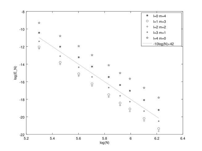
Figure 2: Convergence curves, with $u(x)=x(1-x)e^{4\cos(41x)}$ and $E_{N}:=\|\mathbf{u}^{N}-\mathbf{u}^{N,ex}\|_{\infty}$, $N\in\{200,235,271,300,341,372,401,447,500\}$, for the optimal schemes designed in Proposition 2.6, with $n=10$, $\mu=8$, $d=d^{l,m}$ and $s=s^{l,m}$.

As explained in the introduction, we now address the question of generic performance of the schemes that we have constructed above: are they stable and convergent in general once the algebraic order conditions are satisfied. To give a meaning to this question, we decide to use measure theory. Of course there exist formulas such that $(\mathbf{D}_{N}(d))_{N}$ can not be stable. It is the case, for example, when $\mathbf{D}_{N}(d)$ is not invertible for all $N$ which occurs for when the polynomial $P$ defining the scheme admit a root of the form $4\sin^{2}\left(\frac{\pi}{2}kh\right)$, see (23), which are eigenvalues of the matrix $\mathbf{A}_{N}$. But even if this is not the case, these eigenvalues can be very close to the roots of $P$, which induces small denominators in the stability estimates. Of course, these situations have to be avoided as well.

The following theorem gives an answer to these questions (see Application 1 of Theorem 4.1 and Application 2 of Theorem 4.3 for the proof).

Theorem 2.9.

Let $\mathbb{K}\in\{\mathbb{R},\mathbb{C}\}$ be a field and $l\in\mathbb{N}$ be an integer. Let $\mathscr{C}_{\mathbb{K},l}$ be the $\mathbb{K}$ finite dimensional vector space of symmetric formulas $d\in\mathscr{S}_{\mathbb{K}}$ with zero mean (16) and $\tau(d)\leq l+1$

$$\mathscr{C}_{\mathbb{K},l}=\{d\in\mathscr{S}_{\mathbb{K}}\ |\ \sum_{j\in\mathbb{Z}}d_{j}=0\textrm{ and }\tau(d)\leq l+1\}.$$

Then for any Lebesgue measure on $\mathscr{C}_{\mathbb{K},l}$, we have that:

• For almost all $d\in\mathscr{C}_{\mathbb{C},l}$, $(\mathbf{D}_{N}(d))_{N\in\mathbb{N}^{*}}$ is strongly stable (9).

• For almost all $d\in\mathscr{C}_{\mathbb{R},l}$, $(\mathbf{D}_{N}(d))_{N\in\mathbb{N}^{*}}$ is stable relatively to any sequence $(\eta_{N})_{N}$ (10) such that

  $$\sum_{N\in\mathbb{N}^{*}}\frac{N+1}{\eta_{N}}<\infty\textrm{ and }\sup_{N\in\mathbb{N}^{*}}\frac{(N+1)^{2}}{\eta_{N}}<\infty.$$

As for Bertrand series, there is no optimal choice of sequence $(\eta_{N})_{N\in\mathbb{N}}$ that satisfy this condition and we can not directly deduce stability in the sense of (8), but we can choose

$$\eta_{N}=((N+1)\log(N+1))^{2}=\left(\frac{\log h}{h}\right)^{2}.$$

As a consequence, we affirm that, up to some logarithmic corrections, almost all real symmetric formula generates stable schemes.

We use this theorem to deduce a convergence result.

Proposition 2.10.

With any given $d\in\mathscr{C}_{\mathbb{K},l}$, we can associate the scheme of Proposition 2.6, with $\mu=n-2$ if $\mathbb{K}=\mathbb{C}$ and $\mu=n$ if $\mathbb{K}=\mathbb{R}$, and the formula $s$ given by Proposition 2.2. Then, it follows from Theorem 2.1 that for all $l\in\mathbb{N}$,

• for almost all $d\in\mathscr{C}_{\mathbb{C},l}$, the associated scheme is convergent of order $n$.

• for almost all $d\in\mathscr{C}_{\mathbb{R},l}$, the associated scheme converges at the rate $h^{n}(\log(h))^{2}$.

In the proof of Theorem 2.9 for real formulas, the logarithmic correction is due to the use of a diophantine control of some resonances. Experimentally, we can indeed evidence these quasi-resonances by plotting convergence curves for various schemes of Proposition 2.10 for randomly drawn formulas $d$. Two typical kinds of behaviors for the convergence curves can be observed (see Figures 3 and 4 below). For random $d$, either we observe classical convergence curves (which are close to straight lines and correspond to non-resonant situations), or we obtain strange curves with a complex behaviour corresponding to close to resonant situations.

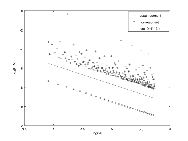
Figure 3: Convergence curves with $u(x)=x(1-x)e^{2x}$ , $n=2$ and $E_{N}:=\|\mathbf{u}^{N}-\mathbf{u}^{N,ex}\|_{\infty}$. For the non-resonant scheme $d=2\mathbb{1}_{\{0\}}-\mathbb{1}_{\{-1,1\}}$ and for the quasi-resonant scheme $d=(2-6z)\mathbb{1}_{\{0\}}+(4z-1)\mathbb{1}_{\{-1,1\}}-z\mathbb{1}_{\{-2,2\}}$ with $z=0.358946420670826$.

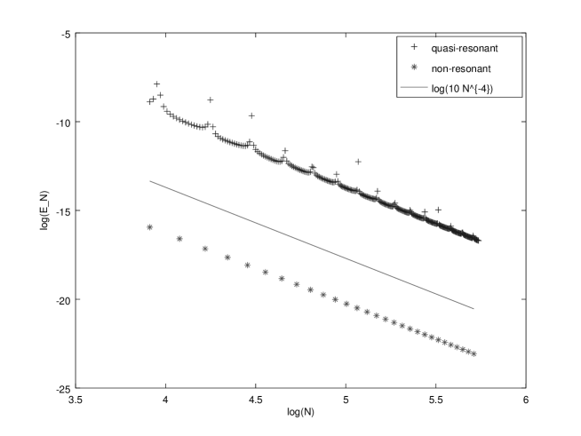
Figure 4: Convergence curves with $u(x)=x(1-x)e^{2x}$ , $n=4$ and $E_{N}:=\|\mathbf{u}^{N}-\mathbf{u}^{N,ex}\|_{\infty}$. For the non-resonant scheme $d=2\mathbb{1}_{\{0\}}-\mathbb{1}_{\{-1,1\}}$ and for the quasi-resonant scheme $d=(2-6z)\mathbb{1}_{\{0\}}+(4z-1)\mathbb{1}_{\{-1,1\}}-z\mathbb{1}_{\{-2,2\}}$ with $z=32.12121212$.

3 Polynomials and high order formulas

The aim of this section is two fold. First, to explain why the matrices $\mathbf{D}_{N}(d)$ constructed in Proposition 2.6 are polynomials in $d$. Second, to give criteria of consistency on these polynomials to interpret Theorem 2.7 as a classical problem of Padé approximant.

To highlight the algebraic structure of the matrices $\mathbf{D}_{N}(d)$ of Proposition 2.6 we will now give a more formal definition of these matrices.

Let $d\in\mathscr{S}_{\mathbb{C}}$ be a symmetric formula. We introduce $T_{d}\in\mathscr{L}(\mathbb{C}^{\mathbb{Z}})$, the operator of convolution by $d$,

$$\forall w\in\mathbb{C}^{\mathbb{Z}},\ T_{d}(w)=d\star w=\left(\sum_{j\in\mathbb{Z}}d_{j}w_{i-j}\right)_{i\in\mathbb{Z}}.$$ (28)

Let $N\in\mathbb{N}^{*}$ and $\mathscr{E}_{N}$ be the space of the odd functions from $\mathbb{Z}$ to $\mathbb{C}$ that are odd in $0$ and in $N+1$

$$\mathscr{E}_{N}:=\{w\in\mathbb{C}^{\mathbb{Z}}\ |\ \forall j\in\mathbb{Z},\ w_{N+1+j}=-w_{N+1-j}\textrm{ and }w_{-j}=-w_{j}\}.$$ (29)

Let $\mathscr{B}_{N}$ be the canonical basis of $\mathscr{E}_{N}$

$$\mathscr{B}_{N}=(\mathbb{1}_{j+(2N+2)\mathbb{Z}}-\mathbb{1}_{-j+(2N+2)\mathbb{Z}})_{j=1,\dots,N}.$$ (30)

Since $d$ is symmetric, we verify that $\mathscr{E}_{N}$ is stable by $T_{d}$.

Definition 3.1.

With the previous construction, we define $\mathbf{D}_{N}(d)$ through the relation

$$\mathbf{D}_{N}(d)=\operatorname{mat}_{\mathscr{B}_{N}}T_{d|\ \mathscr{E}_{N}}.$$

Remark 3.2.

Of course, this definition of $\mathbf{D}_{N}(d)$ gives the same matrices, when $N$ is large enough, as the matrix of Proposition 2.6.

The space of symmetric formulas has a structure of free module on the ring of polynomial that is very useful to write efficient and accurate high order schemes. More precisely, we equip the set of formula $\mathbb{C}^{(\mathbb{Z})}$ of its structure of commutative algebra for the convolution

$$\forall d,s\in\mathbb{C}^{(\mathbb{Z})},\ d\star s=\left(\sum_{j\in\mathbb{Z}}d_{j}s_{i-j}\right)_{i\in\mathbb{Z}}.$$

Then, if $R$ is a ring such that $\mathbb{Z}\subset R\subset\mathbb{C}$, we consider $\mathscr{S}_{R}$ as a subalgebra of $\mathbb{C}^{(\mathbb{Z})}$.

On the one hand, this structure explains, through the following lemma, the importance of the formula $a$ (defined in (12) by $a=2\mathbb{1}_{\{0\}}-\mathbb{1}_{\{-1,1\}}$).

Lemma 3.3.

If $R$ is a ring such that $\mathbb{Z}\subset R\subset\mathbb{C}$ then $\mathscr{S}_{R}$ is a free $R[X]$ module whose $a$ is a basis

$$\forall d\in\mathscr{S}_{R},\ \exists\ !\ P\in R[X],\ d=P(a).$$

Furthermore, if $P\in\mathbb{C}[X]$ then

$$\tau(P(a))=\deg P.$$

Proof.

If we consider $\mathbb{C}^{(\mathbb{Z})}$ as a subalgebra of $\mathbb{C}^{\left(\frac{\mathbb{Z}}{2}\right)}$ then we remark that

$$a=-\left(\mathbb{1}_{\left\{\frac{1}{2}\right\}}-\mathbb{1}_{\left\{-\frac{1}{2}\right\}}\right)^{\star 2}.$$

Consequently, a binomial expansion gives

$$\forall n\in\mathbb{N},\ a^{\star n}=(-1)^{n}\left(\mathbb{1}_{\left\{\frac{1}{2}\right\}}-\mathbb{1}_{\left\{-\frac{1}{2}\right\}}\right)^{\star 2n}=\sum_{k=0}^{n}\frac{(2n)!}{(n+k)!(n-k)!}(-1)^{k}\mathbb{1}_{\{k,-k\}}.$$

The second point of the lemma is clearly a consequence of this expansion. Furthermore, since the term associated to the highest index of $a^{\star n}$ (i.e. $(-1)^{n}$) is invertible in $R$, the first point follows from an induction. ∎

On the other hand, this structure explains, why the matrices $\mathbf{D}_{N}(d)$ are polynomials in $\mathbf{A}_{N}$.

Lemma 3.4.

For all $N\in\mathbb{N}^{*}$, $d\mapsto\mathbf{D}_{N}(d)$ is a $\mathbb{C}[X]$ module morphism:

$$\forall P\in\mathbb{C}[X],\forall d\in\mathscr{S}_{\mathbb{C}},\ \mathbf{D}_{N}(P(d))=P(\mathbf{D}_{N}(d)).$$

Proof.

It follows directly of Definition 3.1 of $\mathbf{D}_{N}(d)$ and of the associativity of the convolution. ∎

3.1 Consistency for the polynomials

We start with a lemma that we have used implicitly in the introduction (in Proposition (2.2) and Proposition (2.4)).

Lemma 3.5.

Let $n\in 2\mathbb{N}$. Then a couple of formulas $(d,s)\in\mathscr{S}_{\mathbb{C}}^{2}$ is consistent of order $n$ (11) if and only if

$$\forall p\in\mathbb{C}_{n+1}[X],\ \sum_{j\in\mathbb{Z}}d_{j}p(j)+s_{j}p^{\prime\prime}(j)=0.$$

Proof.

It is enough to choose $u(x)=x^{i}$ with $i\leq n+1$ is the definition of the consistency and then to simplify the powers of "$h$". Conversely, it is enough to do a Taylor expansion. ∎

In particular, if we choose $p=1$, we find that the consistency of order $n=0$ is nothing but the condition of zero mean (16) for $d$.

We introduce the formal Fourier transform $\mathscr{F}$ from the algebra of formulas $\mathbb{C}^{(\mathbb{Z})}$ to the algebra of formal series $\mathbb{C}\llbracket X\rrbracket$ defined by

$$\mathscr{F}:\left\{\begin{array}[]{llll}\mathbb{C}^{(\mathbb{Z})}&\to&\mathbb{C}\llbracket X\rrbracket\\ d&\mapsto&\displaystyle\sum_{j\in\mathbb{Z}}d_{j}e^{ijX}.\end{array}\right.$$

We give a characterization of consistency through this transform.

Lemma 3.6.

Let $n\in 2\mathbb{N}$. A couple of formulas $(d,s)\in\mathscr{S}_{\mathbb{C}}^{2}$ is consistent of order $n$ (11) if and only if

$$\mathscr{F}d=X^{2}\mathscr{F}s\mod X^{n+2}.$$

Proof.

Let $\partial_{X}\in\mathscr{L}(\mathbb{C}[X])$ be the formal derivative on the space of the polynomials $\mathbb{C}[X]$. As a consequence, since the Taylor expansion in $0$ of a polynomial is exact, if $p\in\mathbb{C}[X]$ and $x_{0}\in\mathbb{C}$ then we have

$$p(x_{0})=e^{x_{0}\partial_{X}}p(0).$$

Consequently, following Lemma (3.5), $(d,s)\in\mathscr{S}_{\mathbb{C}}^{2}$ is consistent of order $n$ (11) if and only if

$$\forall p\in\mathbb{C}_{n+1}[X],\ \left(\mathscr{F}d-X^{2}\mathscr{F}s\right)(i\partial_{X})p(0)=0.$$

We conclude the proof by considering the lowest power in the expansion of $\mathscr{F}d-X^{2}\mathscr{F}s$ in $0$. ∎

The formal Fourier transform is as usual an algebra morphism. As a consequence, if $P\in\mathbb{C}[X]$ and $d=P(a)$ then

$$\sum_{k\in\mathbb{N}^{*}}\sum_{j\in\mathbb{Z}}d_{j}\frac{(-1)^{k}j^{2k}}{(2k)!}X^{2k}=\mathscr{F}d=P(\mathscr{F}a)=P(2-2\cos(X))=P\left(4\sin^{2}\left(\frac{X}{2}\right)\right).$$ (31)

The consistency and the stability of the formulas often involve moment of $d$ or $s$. In particular, this relation provides simple expressions for the first moments of $d$ in function of $P$

$$\sum_{j\in\mathbb{Z}}d_{j}=P(0)\textrm{ and }\sum_{j\in\mathbb{Z}}d_{j}j^{2}=-2P^{\prime}(0).$$

In fact, with the formula (31), we get a criterion of consistency directly on the polynomials.

Lemma 3.7.

Let $P,Q\in\mathbb{C}[X]$ and $n\in 2\mathbb{N}^{*}$. The couple of symmetric formulas $(P(a),Q(a))$ is consistent of order $n$ (11) if and only if

$$P(4X^{2})=4\left(\arcsin(X)\right)^{2}Q(4X^{2})\mod X^{n+2},$$

where $\left(\arcsin(X)\right)^{2}$ is the square of the inverse sine function whose expansion is (for a reference, see, for example, [2])

$$\left(\arcsin(X)\right)^{2}=\sum_{n\in\mathbb{N}^{*}}\frac{2^{2n-1}}{n^{2}C_{2n}^{n}}X^{2n}.$$

Proof.

If we apply (31) to the criterion of consistency of Lemma 3.6 then it comes

$$P\left(4\sin^{2}\left(\frac{X}{2}\right)\right)=X^{2}Q\left(4\sin^{2}\left(\frac{X}{2}\right)\right)\mod X^{n+2}.$$

To conclude the proof, it is enough to do the change of variable

$$X\leftarrow 2\arcsin(X).$$

∎

3.2 The optimal case

In order to prove Theorem 2.7 we are going to explain the link between the problem of optimization (26) and the theory of Padé approximant. To see this link we introduce the usual valuation on $\mathbb{C}\llbracket X\rrbracket$:

$$\forall C\in\mathbb{C}\llbracket X\rrbracket,\ {\rm val}(C)=\min\{k\in\mathbb{N}\ |\ \forall 0\leq j\leq k,\ C^{(j)}(0)=0\}.$$

As a consequence, with this formalism, Lemma 3.7 can be written

$$\forall P,Q\in\mathbb{C}[X],\ \operatorname{ord}\left(P(a),Q(a)\right)={\rm val}\left(P(4X^{2})-4\left(\arcsin(X)\right)^{2}Q(4X^{2})\right)-2.$$

However, Lemma 3.3 proves that $(P,Q)\mapsto(P(a),Q(a))$ is a bijection from $\mathbb{C}_{l+1}[X]\times\mathbb{C}_{m}[X]$ to the space of the couples of symmetric formulas $(d,s)$ such that $\tau(d)\leq l+1$ and $\tau(s)\leq m$. As a consequence, the problem of optimization (26) is equivalent to the following

$$\mathop{\max_{(P,Q)\in\mathbb{C}[X]^{2}\setminus\{(0,0)\}}}_{\deg P\leq l+1,\ \deg Q\leq m}{\rm val}\left(P(4X^{2})-4\left(\arcsin(X)\right)^{2}Q(4X^{2})\right).$$

Since if $P(0)\neq 0$ then ${\rm val}\left(P(4X^{2})-4\left(\arcsin(X)\right)^{2}Q(4X^{2})\right)=0$, it is natural to study this problem of optimization for polynomials $P$ such that

$$P=XR\textrm{ where }R\in\mathbb{C}_{l}[X].$$

Consequently, it is enough to study the following problem of optimization

$$\mathop{\max_{(R,Q)\in\mathbb{C}[X]^{2}\setminus\{(0,0)\}}}_{\deg R\leq l,\ \deg Q\leq m}{\rm val}\left(R-CQ\right),$$ (32)

with (see [2] for the expansion)

$$C(X):=4\left(\frac{\arcsin(\frac{\sqrt{X}}{2})}{\sqrt{X}}\right)^{2}=2\sum_{n\in\mathbb{N}}\frac{X^{n}}{(n+1)^{2}C_{2n+2}^{n+1}}.$$ (33)

The theory of Padé approximants is a deep theory about approximation of formal series by rational ones. It has been extensively developed in the last decades (see [1] or [4] for an overview). Its aim is to give to each formal series $F\in\mathbb{C}\llbracket X\rrbracket$ a rational approximation $\frac{p_{l,m}}{q_{l,m}}$ (usually noted $[l/m]$) such that

$$F=\frac{p_{l,m}}{q_{l,m}}\mod X^{l+m+1}\textrm{ , with }p_{l,m}\in\mathbb{C}_{l}[X]\textrm{ and }q_{l,m}\in\mathbb{C}_{m}[X].$$ (34)

A natural way to find such an approximation is to try to solve

$$p_{l,m}=Fq_{l,m}\mod X^{l+m+1}\textrm{ , with }p_{l,m}\in\mathbb{C}_{l}[X]\textrm{ and }q_{l,m}\in\mathbb{C}_{m}[X].$$ (35)

Indeed, if we get a solution $(p_{l,m},q_{l,m})$ of (35) with $q_{l,m}(0)\neq 0$ then it is also a solution of (34). The second formulation (35) is interesting because it is a linear system of $l+m+1$ equations and $l+m+2$ unknowns. Consequently, it admits at least one non trivial solution. However, the question of its uniqueness (up to multiplication by a scalar) is generaly non trivial. In the classical Padé theory, if for a formal series $F$, the linear system (35) admits for all $l,m\in\mathbb{N}$, a unique non trivial solution (up to multiplication by a scalar), then it is said that the Padé table of $F$ is normal. Furthermore, if $F(0)\neq 0$ and if its Padé table is normal then a non trivial solution $(p_{l,m},q_{l,m})$ of (35) satisfies $\deg p_{l,m}=l$, $\deg q_{l,m}=m$, $q_{l,m}(0)\neq 0$ and ${\rm val}(p_{l,m}-Fq_{l,m})=l+m+1$ (see [1] or [4] for details).

What is crucial for us is that the Padé table of $C$ is normal. In fact, D. Karp and E. Prilepkina have proved in [7] that the Padé tables of many generalized hypergeometric functions are normals. To see that the Padé table of $C$ is normal, we just have to verify that $C$ is one of those generalized hypergeometric functions. The generalized hypergeometric functions are the formal series defined by

$${}_{p}F_{q}\biggl{[}\genfrac{.}{.}{0.0pt}{}{\alpha_{1}\mskip 8.0mu\dots\mskip 8.0mu\alpha_{p}}{\beta_{1}\mskip 8.0mu\dots\mskip 8.0mu\beta_{q}};X\biggr{]}=\sum_{k\in\mathbb{N}}\frac{(\alpha_{1})_{k}\dots(\alpha_{p})_{k}}{(\beta)_{1}\dots(\beta_{q})_{k}}\frac{X^{k}}{k!}\textrm{ with }(\gamma)_{k}=\prod_{j=0}^{k-1}\gamma+j.$$ (36)

D. Karp and E. Prilepkina have proved in Theorem $9$ of [7] that if

$$\left\{\begin{array}[]{lll}p=q+1,\\ 0<\alpha_{q+1}\leq 1,\\ 0<\alpha_{1}\leq\dots\leq\alpha_{q},\\ 0<\beta_{1}\leq\dots\leq\beta_{q},\\ \forall k\in\llbracket 1,q\rrbracket,\ \displaystyle\sum_{j=1}^{k}\alpha_{j}\leq\sum_{j=1}^{k}\beta_{j}\end{array}\right.$$

then the Padé table of ${}_{p}F_{q}\biggl{[}\genfrac{.}{.}{0.0pt}{}{\alpha_{1}\mskip 8.0mu\dots\mskip 8.0mu\alpha_{p}}{\beta_{1}\mskip 8.0mu\dots\mskip 8.0mu\beta_{q}};X\biggr{]}$ is normal. However, $C$ is one of those generalized hypergeometric functions because

$$C(X)={}_{3}F_{2}\biggl{[}\genfrac{.}{.}{0.0pt}{}{1\mskip 8.0mu1\mskip 8.0mu1}{\frac{3}{2}\mskip 8.0mu2};\frac{X}{4}\biggr{]}.$$ (37)

We verify this assertion by the following elementary calculation

$$\frac{(n+1)^{2}C_{2n+2}^{n+1}}{(n+2)^{2}C_{2n+4}^{n+2}}=\frac{(n+1)^{2}}{(2n+3)(2n+4)}=\frac{1}{4}\frac{(n+1)^{2}}{(n+\frac{3}{2})(n+2)},$$

which shows by induction that the coefficients of $C(X)$ (see (33)) coincide with those of one of the generalized hypergeometric functions in (37), see (36).

Now, we just have to link these results of Padé approximation with our optimization problem (26). But if we denote by $(R_{l,m},Q_{l,m})$ the solution of (35) such that $R_{l,m}(0)=1$, then we have

$${\rm val}(R_{l,m}-CRQ_{l,m})=l+m+1.$$

Conversely, if $(R,Q)$ satisfyies ${\rm val}(R-CRQ)\geq l+m+1$ with $\deg R\leq l$ and $\deg Q\leq m$ then it is a solution of (35). But since the Padé table of $C$ is normal, $(R,Q)$ is equal to $(R_{l,m},Q_{l,m})$, up to multiplication by a scalar.

Consequently, we have proved that the numerator and the denominator of the Padé approximant of $C$ are the solutions to the optimization problem (32), up to multiplication by a scalar. All the results of this analysis is summarized in the following theorem that is nothing but a version of Theorem 2.7 with polynomials.

Theorem 3.8.

For all $l,m\in\mathbb{N}$, there exists a couple of rational polynomial $(R_{l,m},Q_{l,m})\in\mathbb{Q}[X]^{2}$ such that

$$\left\{\begin{array}[]{llll}\deg R_{l,m}=l,\\ \deg Q_{l,m}=m,\\ R_{l,m}(0)=1.\end{array}\right.$$

Moreover $(R_{l,m},Q_{l,m})$ is solution of the optimization problem

$$\mathop{\max_{(R,Q)\in\mathbb{C}[X]^{2}\setminus\{(0,0)\}}}_{\deg R\leq l,\ \deg Q\leq m}{\rm val}\left(R-CQ\right)={\rm val}\left(R_{l,m}-CQ_{l,m}\right)=l+m+1.$$

Furthermore, this solution is essentially unique: if $(R,S)\in\mathbb{C}[X]^{2}$ is such that $\deg R\leq l$, $\deg Q\leq m$ and ${\rm val}\left(R_{l,m}-CQ_{l,m}\right)=l+m+1$ then there exists $\lambda\in\mathbb{C}$ such that $R=\lambda R_{l,m}$ and $Q=\lambda Q_{l,m}$.

There exists many very efficient methods to compute effectively Padé approximants (see for example [1] or [4]). Consequently, if the order of consistency is large enough, it is interesting to not compute the optimal formulas of Theorem 2.7 through the resolution of the linear system (27), but to compute them from the optimal polynomials of Theorem 3.8 through the relations

$$s^{l,m}=Q_{l,m}(a)\textrm{ and }d^{l,m}=P_{l,m}(a)\textrm{ with }P_{l,m}(X)=XR_{l,m}(X).$$ (38)

4 Stability

In this section we study criteria of stability for the sequences of matrices of the form $P(\mathbf{A}_{N})$ with $P$ a polynomial. These conditions hold on the polynomial $P$. As a consequence, if we want to apply one of these criteria to a matrix of the form $\mathbf{D}_{N}(d)$, with $d$ a symmetric formula, we have to solve $P(a)=d$ (see Lemma 3.3 for details).

In the first part, we give a criterion of strong stability (9) and then we deduce Theorem 2.8 and the first part of Theorem 2.9 (when the formulas are complex). In the second part, we give a diophantine criterion of relative stability (10) that is enough to prove the second part of Theorem 2.9 (when the formulas are real).

4.1 Strong stability

Theorem 4.1.

Let $P\in\mathbb{C}[X]$ be a polynomial such that

$$P(0)=0,\ P^{\prime}(0)\neq 0\textrm{ and }\forall x\in]0,4],\ P(x)\neq 0.$$ (39)

Then the sequence of matrices $(P(\mathbf{A}_{N}))_{N\in\mathbb{N}^{*}}$ is strongly stable (9).

Proof.

The assumptions (39) implies that there exists $\beta\neq 0$ a real number and a sequence $(\mu_{k})_{k=1\dots d}$ of complex numbers such that

$$P(X)=\beta X\prod_{k=1}^{d}\left(X-\mu_{k}\right).$$

On the one hand, a straightforward calculation shows that $\mathbf{A}_{N}$ is invertible and

$$\forall i,j\in\llbracket 1,N\rrbracket,\ (\mathbf{A}_{N}^{-1})_{i,j}=\min(j(1-hi),i(1-hj)).$$

On the other hand, since by assumption $\mu_{k}\notin[0,4]$, the following lemma (proved in Appendix 5.2) shows that $\mathbf{A}_{N}-\mu_{k}\mathbf{I}_{N}$ is invertible and that there exists a constant $c_{\mu_{k}}$ such that for all $N$, $\|(\mathbf{A}_{N}-\mu_{k}\mathbf{I}_{N})^{-1}\|_{\infty}\leq c_{\mu_{k}}$.

Lemma 4.2.

If $\mu\in\mathbb{C}\setminus[0,4]$ then there exists $c>0$ such that for all $N\in\mathbb{N}^{*}$, $\mathbf{A}_{N}-\mu\mathbf{I}_{N}$ is invertible and for all $\mathbf{v}\in\mathbb{C}^{N}$

$$\|\mathbf{v}\|_{\infty}\leq c\|\mathbf{A}_{N}\mathbf{v}-\mu\mathbf{v}\|_{\infty}.$$

As a consequence, $P(\mathbf{A}_{N})$ is invertible and we have

$$\forall N\in\mathbb{N}^{*},\forall\mathbf{v}\in\mathbb{R}^{N},\ \|P(\mathbf{A}_{N})^{-1}\mathbf{v}\|_{\infty}\leq|\beta|^{-1}\|\mathbf{A}_{N}^{-1}\mathbf{v}\|_{\infty}\prod_{k=1}^{d}c_{\mu_{k}}.$$

Hence, to prove Theorem 4.1, it is enough to prove that $(\mathbf{A}_{N})_{N}$ is strongly stable (9). The estimation of strong stability of $(\mathbf{A}_{N})_{N}$ is very explicit and is given for $l\in\mathbb{N}$ by

$$\|\mathbf{A}_{N}^{-1}\mathbf{v}\|_{\infty}$$

$$\leq\sup_{i=1}^{N}\sum_{j=1}^{N}|\mathbf{v}_{j}|\min\{i(1-hj),j(1-hi)\}$$

$$\leq\sup_{i=1}^{N}\sum_{j\in\llbracket l+1,N-l\rrbracket}|\mathbf{v}_{j}|\min\{i(1-hj),j(1-hi)\}+\sup_{i=1}^{N}\sum_{j\in\llbracket l+1,N-l\rrbracket^{c}}|\mathbf{v}_{j}|\min\{i(1-hj),j(1-hi)\}$$

$$\leq\sup_{i=1}^{N}\sum_{j\in\llbracket l+1,N-l\rrbracket}|\mathbf{v}_{j}|\frac{4}{h}+\sup_{i=1}^{N}\sum_{j\in\llbracket l+1,N-l\rrbracket^{c}}|\mathbf{v}_{j}|l$$

$$\leq\sup_{j=1}^{N}\left\{\begin{array}[]{lll}4h^{-2}|\mathbf{v}_{j}|&\textrm{ if }l+1\leq j\leq N-l,\\ 2l^{2}|\mathbf{v}_{j}|&\textrm{ else.}\end{array}\right.$$

∎

Application 1: Proof of the first part of Theorem 2.9.
The more direct application of this criterion of strong stability is the first part of Theorem 2.9. Since we have proved in Lemma 3.3 that $P\mapsto P(a)$ induce an isomorphism of vector space between $X\mathbb{C}_{l}[X]$ and $\mathscr{C}_{\mathbb{C},l}$, it is enough to prove that almost all complex polynomials of degree smaller than $l+1$ do not have any zero point in $[0,4]$ to conclude with the criterion of stability of Theorem 4.1. In fact, we show that almost all complex polynomials of degree smaller than $l+1$ do not have any real zero point.

Proof.

Since the null sets are the same for all the Lebesgue measures on $\mathbb{C}_{l}[X]$ it is enough to prove the result for one well chosen Lebesgue measure. As a consequence, we introduce $\lambda$ be a Lebesgue measure on $\mathbb{R}_{l}[X]$ and we consider $\lambda^{\otimes 2}$ as a Lebesgue measure on $\mathbb{C}_{l}[X]$ induced by the direct sum

$$\mathbb{C}_{l}[X]=\mathbb{R}_{l}[X]\oplus i\mathbb{R}_{l}[X].$$

Now, we remark that if a polynomial $P\in\mathbb{C}_{l}[X]$ admits the decomposition $P=P_{1}+iP_{2}$ and has a real zero point $x\in\mathbb{R}$ then $x$ is a zero point of $P_{1}$ and of $P_{2}$. As a consequence, we conclude by the following calculation

$$\lambda^{\otimes 2}\{P\in\mathbb{C}_{l}[X]\ |\ \exists x\in\mathbb{R},\ P(x)=0\} =\int_{\mathbb{R}_{l}[X]}\int_{\mathbb{R}_{l}[X]}\mathbb{1}_{\exists x\in\mathbb{R},\ (P_{1}+iP_{2})(x)=0}{\rm d\lambda(P_{1})}{\rm d\lambda(P_{2})}$$

$$=\int_{\mathbb{R}_{l}[X]}\int_{\mathbb{R}_{l}[X]}\mathbb{1}_{\exists x\in\mathbb{R},\ P_{2}(x)=P_{1}(x)=0}{\rm d\lambda(P_{1})}{\rm d\lambda(P_{2})}$$

$$\leq\int_{\mathbb{R}_{l}[X]}\sum_{x\in\mathbb{R},P_{2}(x)=0}\int_{\mathbb{R}_{l}[X]}\mathbb{1}_{P_{1}(x)=0}{\rm d\lambda(P_{1})}{\rm d\lambda(P_{2})}$$

$$=0.$$

The last equality is nothing but, since $\{P_{1}\in\mathbb{R}_{l}[X]|\ P_{1}(x)=0\}$ is an hyperplane of $\mathbb{R}_{l}[X]$, its Lebesgue measure is zero. ∎

Application 2: Proof of Theorem 2.8 .
The second application of the criterion of strong stability of Theorem 4.1 is the Theorem 2.8 about the strong stability of the most efficient schemes. In fact, to apply this criterion to the optimal formulas of Theorem 2.7, we exactly have to prove that the optimal polynomials $R_{l,m}$ of Theorem 3.8 do not have any zeros point in $[0,4]$.

Proof.

Let $l,m\in\mathbb{N}$ be some integers and $R_{l,m}$ the optimal polynomial given by Theorem 3.8. In the proof of this theorem, $R_{l,m}$ is built as the numerator of the Padé approximant of the function $C$ (33). Futhermore, as we have explained in the proof of Theorem 3.8, D. Karp and E. Prilepkina have proved in [7] that $C(-X)$ is a Stieltjes transform of a measure supported in $[0,4]$. As a consequence, we can use the classical results about the localization of the zeros points and poles of the Padé approximants of such series.

On the one hand, it is enough to apply the point $(vii)$ of Theorem $3$ page $251$ of the book of J. Gilewicz [4] to prove that if $k\leq 0$ and $l\geq-k$ then all the zero points of $R_{l+k,l}$ are in $]4,\infty[$.

On the other hand, J. Gilewicz proves at the point $(iii)$ of this theorem that if $k\geq-1$, $l+k\geq 0$ and $l\geq 0$ then all the zero points of $Q_{l+k,l}$ (the denominator of the Padé approximant of $C$) are in $]4,\infty[$. Futhermore, page $264$ of his book [4], J. Gilewicz gives a theorem of Stieltjes and Wynn (point $(iii)$ of Theorem $5$) that implies that if $k\geq 0$ and $l\leq 0$ then

$$\forall x\in[0,4],\ \frac{R_{l+k,l}(x)}{Q_{l+k,l}(x)}\leq\frac{R_{l+k+1,l+1}(x)}{Q_{l+k+1,l+1}(x)}.$$

Since $Q_{l+k,l}$ does not have any zero point on $[0,4]$ and since by construction $Q_{l+k,l}(0)=R_{l+k,l}(0)=1$ then it follows that for all $k\geq 0$ and all $l\geq 0$ we have

$$\forall x\in[0,4],\ Q_{l+k,l}(x)>0.$$

As a consequence, if $k\geq 0$ and $l\geq 0$ then, we have

$$\forall x\in[0,4],\ \frac{Q_{l+k+1,l+1}(x)}{Q_{l+k,l}(x)}R_{l+k,l}(x)\leq R_{l+k+1,l+1}(x).$$

Consequently, if for all $k\geq 0$, we prove that $R_{k,0}$ is positive on $[0,4]$, then we conclude by induction on $l\geq 0$, that $R_{l+k,l}$ is positive on $[0,4]$. Indeed, it is clear that $R_{k,0}$ is positive on $[0,4]$ because by construction (see Theorem 3.8), we have

$$R_{k,0}=2\sum_{n=0}^{k}\frac{X^{n}}{(n+1)^{2}C_{2n+2}^{n+1}}>0\textrm{ on }\mathbb{R}^{+}.$$

∎

4.2 Relative stability

Theorem 4.3.

Let $P\in\mathbb{C}[X]$ be a polynomial and let $\Lambda$ be the set of the roots of $P$ in $[0,4]$ and assume that $P$ satisfies the following assumptions:

1. $0\in\Lambda$,

2. $4\notin\Lambda$,

3. the roots of $P$ in $[0,4]$ are simple,

4. $\exists\delta:\mathbb{N}^{*}\to\mathbb{R}_{+}^{*}$,

   $$\forall\lambda\in\Lambda,\forall q\in\mathbb{N}^{*},\forall 1\leq p\leq q-1,\ \ 0<\delta_{q}\leq\left|\lambda-4\sin^{2}\left(\frac{\pi}{2}\frac{p}{q}\right)\right|.$$ (40)

Then the sequence of finite difference matrices $(P(\mathbf{A}_{N}))_{N\in\mathbb{N}^{*}}$ is stable relatively to the sequence $\eta_{N}=\frac{1}{\delta_{N+1}}$ (10).

Proof.

see Appendix 5.3. ∎

Application 1: stability for second order algebraic zero points
The first application of this diophantine criteria is based on a classical result about approximation of algebraic numbers by rational ones. It gives a way to design sequences of matrices $\mathbf{D}_{N}$ that are stable (8), but such that $\mathbf{D}_{N}$ has not a positive or a negative spectrum for all $N$.

Theorem 4.4.

Liouville’s Theorem. (from the book of Andrei B. Shidlovskii [9] page 23)
If $\alpha$ is a real algebraic number of degree $n$, $n\geq 1$, then there exists a constant $c=c(\alpha)>0$ such that the following inequality holds for any $p\in\mathbb{Z}$ and $q\in\mathbb{N}^{*}$, $\frac{p}{q}\neq\alpha$:

$$\left|\alpha-\frac{p}{q}\right|>\frac{c}{q^{n}}.$$

Corollary 4.5.

If a polynomial $P\in\mathbb{C}[X]$ satisfies the three first hypothesis of Theorem 4.3 and if for all root $\lambda\in\Lambda\setminus\{0\}$ there exist an algebraic number of degree $2$, $\alpha$, such that $\lambda=4\sin^{2}(\frac{\pi}{2}\alpha)$, then the sequence of finite difference matrices $(P(\mathbf{A}_{N}))_{N}$ is stable (8).

Application 2: Proof of the second part of Theorem 2.9.
The proof of the second part of Theorem 2.9 is an adaptation of a classical qualitative result about approximation of real numbers by rational ones.

Theorem 4.6.

A version of the Khinchin’s Theorem. (see for example [9] page 17)
Let $(\nu_{q})_{q}$ be a sequence of positive real numbers such that the series $\sum\nu_{q}$ converges. Then, for almost all $\alpha\in\mathbb{R}$, there exists a constant $c>0$ such that for all $p,q\in\mathbb{Z}\times\mathbb{N}^{*}$, one has

$$|\alpha-\frac{p}{q}|\geq c\frac{\nu_{q}}{q}.$$

More precisely, to prove the second part of Theorem 2.9 with the criterion of Theorem 4.3, it is enough to prove that the following set are null set for a Lebesgue measure on $\mathbb{R}_{l}[X]$ (they are the sets of the polynomials that do not satisfy $ii,iii$ or $iv$):

$$E_{1}=\{R\in\mathbb{R}_{l}[X]\ |\ R(4)=0\textrm{ or }R(0)=0\},$$

$$E_{2}=\{R\in\mathbb{R}_{l}[X]\ |\ \exists\lambda\in[0,4],\ R(\lambda)=R^{\prime}(\lambda)=0\},$$

$$E_{3}=\left\{R\in\mathbb{R}_{l}[X]\ |\ \exists\lambda\in[0,4],\ R(\lambda)=0\textrm{ and }\liminf_{q\to\infty}\min_{p\in\llbracket 1,q-1\rrbracket}\eta_{q-1}\left|\lambda-4\sin^{2}\left(\frac{\pi}{2}\frac{p}{q}\right)\right|=0\right\}.$$

Indeed, since we have proved in Lemma 3.3 that $R\mapsto(XR)(a)$ induce an isomorphism of vector space between $\mathbb{R}_{l}[X]$ and $\mathscr{C}_{\mathbb{R},l}$, the null sets for the Lebesgue measures on $\mathbb{R}_{l}[X]$ are associated to the null sets for the Lebesgue measures on $\mathscr{C}_{\mathbb{R},l}$.

It is quite clear that $E_{1}$ and $E_{2}$ are null sets. Indeed, $E_{1}$ is a null set because since $P\mapsto P(4)$ is linear, it is an hyperplane and $E_{2}$ is a null set because it is the set of the zero points of the discriminant $\Delta(R)=\operatorname{Res}(R,R^{\prime})$ that is a non zero polynomial of $R$. However, to prove that $E_{3}$ is a null set, we have to adapt the proof of the Khinchin’s Theorem 4.6.

In order to use the Borel Cantelli Theorem, we introduce a probability measure $\rho$ on $\mathbb{R}_{l}[X]$ with the same null set as a Lebesgue measure. More precisely, we introduce the Lebesgue measure $\mu$ on $\mathbb{R}_{l}[X]$ induced by the Hardy’s scalar product $\langle.,.\rangle_{\mathcal{H}^{2}}$. This scalar product is defined by

$$\forall R_{1},R_{2}\in\mathbb{R}_{l}[X],\ \langle R_{1},R_{2}\rangle_{\mathcal{H}^{2}}:=\sum_{k=0}^{l}\frac{R_{1}^{(k)}(0)R_{2}^{(k)}(0)}{k!^{2}}.$$

Then, we define $\rho$ through its density with respect to $\mu$

$$\frac{{\rm d\rho}}{{\rm d\mu}}=\frac{1}{\sqrt{2\pi}^{l+1}}e^{-\frac{1}{2}\|R\|_{\mathcal{H}^{2}}^{2}}.$$

As $\rho$ has a positive density with respect to $\mu$, $\rho$ and $\mu$ have the same null sets.
Hence, since $E_{2}$ is a null set, it is enough to prove that $E_{3}\cap E_{2}^{c}$ is a null set. As a consequence, we can use the following inclusion

$$E_{2}^{c}\cap E_{3}\subset E_{2}^{c}\cap\left\{R\in\mathbb{R}_{l}[X]\ |\ \liminf_{q\to\infty}\min_{p\in\llbracket 1,q-1\rrbracket}\eta_{q-1}\left|R\left(4\sin^{2}\left(\frac{\pi}{2}\frac{p}{q}\right)\right)\right|=0\right\}.$$

Then, we introduce the measurable sets

$$F_{q}:=\left\{R\in\mathbb{R}_{l}[X]\ |\ \min_{p\in\llbracket 1,q-1\rrbracket}\left|R\left(4\sin^{2}\left(\frac{\pi}{2}\frac{p}{q}\right)\right)\right|\leq\frac{1}{\eta_{q-1}}\right\},$$

to get the inclusion

$$E_{2}^{c}\cap E_{3}\subset E_{2}^{c}\cap\limsup_{q\to\infty}F_{q}.$$

Consequently, it is enough to prove that $\sum\rho(F_{q})<\infty$ to conclude by the Theorem of Borel Cantelli that $E_{3}$ is a null set.

To control $\rho(F_{q})$, we begin assuming the following lemma, that we will show at the end of this proof.

Lemma 4.7.

For all $\lambda\in\mathbb{R}$ and for all $\beta>0$, we have

$$\rho\left(\left\{R\in\mathbb{R}_{l}[X]\ |\ |R(\lambda)|\leq\beta\right\}\right)\leq\sqrt{\frac{2}{\pi}}\beta.$$

Consequently, we deduce from the last assumption of Theorem 2.9 that $\sum\rho(F_{q})<\infty$,

$$\rho(F_{q}) \leq\sum_{p=1}^{q-1}\rho\left\{R\in\mathbb{R}_{l}[X]\ |\ \left|R\left(4\sin^{2}\left(\frac{\pi}{2}\frac{p}{q}\right)\right)\right|\leq\frac{1}{\eta_{q-1}}\right\}$$

$$\leq(q-1)\sqrt{\frac{2}{\pi}}\frac{1}{\eta_{q-1}}\in l^{1}(\mathbb{N}\setminus\{0,1\})$$

To conclude this proof, we have to prove Lemma 4.7. We introduce the polynomial $R_{\alpha}\in\mathbb{R}_{l}[X]$ defined by

$$R_{\alpha}(X)=\sum_{k=0}^{l}(\alpha X)^{k}.$$

$R_{\alpha}$ is the Riesz representer of the evaluation in $\alpha$

$$\forall R\in\mathbb{R}_{l}[X],\ R(\alpha)=\langle R_{\alpha},R\rangle_{\mathcal{H}^{2}}.$$

Consequently, since the Gaussian measure $\rho$ is isotropic, we have

$$\rho\left(\left\{R\in\mathbb{R}_{l}[X]\ |\ |R(\lambda)|\leq\beta\right\}\right) =\rho\left(\left\{R\in\mathbb{R}_{l}[X]\ |\ |\langle R_{\alpha},R\rangle_{\mathcal{H}^{2}}|\leq\beta\right\}\right)$$

$$=\frac{1}{\sqrt{2\pi}}\int_{\mathbb{R}}\mathbb{1}_{|y|\|R_{\alpha}\|_{\mathcal{H}^{2}}^{2}\leq\beta}e^{-\frac{y^{2}}{2}}{\rm dy}$$

$$\leq\frac{1}{\sqrt{2\pi}}\int_{\mathbb{R}}\mathbb{1}_{|y|\|R_{\alpha}\|_{\mathcal{H}^{2}}^{2}\leq\beta}{\rm dy}$$

$$=\sqrt{\frac{2}{\pi}}\beta\left(\sum_{k=0}^{l}\alpha^{2k}\right)^{-1}\leq\sqrt{\frac{2}{\pi}}\beta.$$

5 Appendix

5.1 Proof of Proposition 2.3

Let $f\in C^{\infty}(\mathbb{R})$ be the source function of the Dirichlet problem (2), and $u$ its solution. For each $N\in\mathbb{N}^{*}$ we consider $\mathbf{u}^{N,ex}$ and $\mathbf{f}^{N,ex}$ the discretizations of $u$ and $f$ defined by (3).

We begin proving the consistency of the scheme in the center. We introduce an integer $j$ such that $\tau(d)<j<N+1-\tau(d)$. Then, we do the estimation of consistency with a Taylor Lagrange formula

$$\left|\left(\mathbf{D}_{N}\mathbf{u}^{N,ex}\right)_{j}-h^{2}\left(\mathbf{S}_{N}\mathbf{f}^{N,ex}\right)_{j}\right|$$

$$=\sum_{i\in\mathbb{Z}}d_{i}u(x^{N}_{i+j})+h^{2}s_{i}u^{\prime\prime}(x^{N}_{i+j})$$

$$=\sum_{i\in\mathbb{Z}}d_{i}p_{j}(x^{N}_{i})+h^{2}s_{i}p_{j}^{\prime\prime}(x^{N}_{i})+\sum_{i\in\mathbb{Z}}d_{i}(\xi^{N,1}_{i,j}-x_{i}^{N})^{n+2}\frac{u^{(n+2)}(\xi^{N,1}_{i,j})}{(n+2)!}+h^{2}s_{i}(\xi^{N,2}_{i,j}-x_{i}^{N})^{n}\frac{u^{(n)}(\xi^{N,2}_{i,j})}{n!},$$

with $\xi^{N,1}_{i,j},\xi^{N,2}_{i,j}\in]x_{i}^{N},x_{i+j}^{N}[$ and

$$p_{j}(X)=\sum_{k=0}^{n+1}\frac{u^{(k)}(x_{j}^{N})}{k!}X^{k}.$$

However, we have proved in Lemma 3.5, that the polynomial part of this sum is zero. Consequently, it is enough to estimate the second part. Finally, we get

$$\left|\left(\mathbf{D}_{N}\mathbf{u}^{N,ex}\right)_{j}-h^{2}\left(\mathbf{S}_{N}\mathbf{f}^{N,ex}\right)_{j}\right| \leq h^{n+2}\|u^{(n+2)}\|_{L^{\infty}(0,1)}\sum_{i\in\mathbb{Z}}|d_{i}|\frac{\tau(d)^{n+2}}{(n+2)!}+|s_{i}|\frac{\tau(s)^{n}}{n!}.$$

The same type of estimations holds near the boundary and we can prove similarly that, if $\tau(d)\geq j$ or $j\geq N+1-\tau(d)$ and if $\frac{\mu h}{2}\leq\gamma$ then

$$\left|\left(\mathbf{D}_{N}\mathbf{u}^{N,ex}\right)_{j}-h^{2}\left(\mathbf{S}_{N}\mathbf{f}^{N,ex}\right)_{j}\right| \leq h^{\mu+2}\|u^{(\mu+2)}\|_{L^{\infty}(-\gamma,1+\gamma)}\max_{1\leq k\leq\tau(d)}\sum_{i\in\mathbb{Z}}|d_{i}^{k}|\frac{\tau(d)^{\mu+2}}{(\mu+2)!}+|s_{i}^{k}|\frac{\tau(s^{k})^{\mu}}{\mu!}.$$

5.2 Proof of Lemma 4.2

To prove this lemma, we need to use the notations introduced to define formally $\mathbf{D}_{N}(d)$ in Definition 3.1.

Now, for all $p\in\mathbb{Z}$ and for all $N\in\mathbb{N}^{*}$, we introduce an operator $O_{p,N}$ on $\mathscr{E}_{N}$ defined by

$$\forall w\in\mathscr{E}_{N},\ O_{p,N}w=\frac{1}{2}T_{\mathbb{1}_{\{p,-p\}}}w=\left(\frac{w_{i+p}+w_{i-p}}{2}\right)_{i\in\mathbb{Z}}.$$

A straightforward calculation shows that the spectral decomposition of $O_{p,N}$ is

$$\forall k\in\mathbb{Z},\ O_{p,N}e_{k,N}=\cos(p\pi kh)e_{k,N}\textrm{ with }e_{k,N}=(\sin(k\pi hj))_{j\in\mathbb{Z}}.$$ (41)

Let $z\in\mathbb{C}\setminus[-1,1]$ be a complex number. Since the periodic function $x\mapsto(\cos(x)-z)^{-1}$ is real analytic, its Fourier transform is summable. More precisely, there exists $(c_{p}(z))\in l^{1}(\mathbb{N})$ such that

$$\forall x\in\mathbb{R},\ \frac{1}{\cos(x)-z}=\sum_{p\in\mathbb{N}}c_{p}(z)\cos(px).$$

Since $(c_{p})$ is summable, it follows from (41) that $O_{1,N}-zI_{\mathscr{E}_{N}}$ is invertible and

$$(O_{1,N}-zI_{\mathscr{E}_{N}})^{-1}=\sum_{p\in\mathbb{N}}c_{p}(z)O_{p,N}.$$

Furthermore, if $w\in\mathscr{E}_{N}$ then for all $p\in\mathbb{N}$

$$\|O_{p,N}w\|_{l^{\infty}(\mathbb{Z})}\leq\|w\|_{l^{\infty}(\mathbb{Z})}.$$

As a consequence, we have

$$\|(O_{1,N}-zI_{\mathscr{E}_{N}})^{-1}w\|_{l^{\infty}(\mathbb{Z})}\leq\sum_{p\in\mathbb{N}}|c_{p}(z)|\|O_{p,N}w\|_{l^{\infty}(\mathbb{Z})}\leq\|(c_{p}(z))\|_{l^{1}(\mathbb{N})}\|w\|_{l^{\infty}(\mathbb{Z})}.$$

To finish the proof of Lemma 4.2, it is enough to see that

$$\operatorname{mat}_{\mathscr{B}_{N}}O_{1,N}=\mathbf{I}_{N}-\frac{1}{2}\mathbf{A}_{N}\textrm{ and }\forall w\in\mathscr{E}_{N},\ \|\operatorname{mat}_{\mathscr{B}_{N}}w\|_{\infty}=\|w\|_{l^{\infty}(\mathbb{Z})}.$$

5.3 Proof of Theorem 4.3

It follows of the spectral decomposition of $\mathbf{A}_{N}$ (22), that $(\mathbf{e}^{N}_{k})_{k=1\dots N}$ is an orthogonal basis of $\mathbb{C}^{N}$. Furthermore, a straightforward calculation shows that, if $k\in\llbracket 1,N\rrbracket$ then we have

$$\|\mathbf{e}^{N}_{k}\|_{2}=\sum_{j=1}^{N}|(\mathbf{e}^{N}_{k})_{j}|^{2}=\sum_{j=1}^{N}\sin^{2}(\pi hkj)=\frac{1}{2}\sum_{j=1}^{N}1-\cos(2\pi hkj)=\frac{1}{2h}.$$

Consequently, if we take a vector $\mathbf{v}\in\mathbb{C}^{N}$, we get its discrete Fourier transform as

$$\mathbf{v}=2h\sum_{k=1}^{N}\mathbf{e}^{N}_{k}\sum_{j=1}^{N}\mathbf{v}_{j}\sin(\pi hkj).$$

However, since the vectors $\mathbf{e}^{N}_{k}$ are eigenvectors of $\mathbf{A}_{N}$, there are eigenvectors of $P(\mathbf{A}_{N})$ and their eigenvalues are $P(4\sin^{2}\left(\frac{\pi}{2}kh\right))$. Consequently, we know from assumption $(iv)$ that $P(\mathbf{A}_{N})$ is invertible and that we have

$$P(\mathbf{A}_{N})^{-1}\mathbf{v}=2h\sum_{k=1}^{N}\frac{e^{N}_{k}}{P\left(4\sin^{2}\left(\frac{\pi}{2}kh\right)\right)}\sum_{j=1}^{N}\mathbf{v}_{j}\sin(\pi hkj).$$

Hence, if we do the estimation, $|\sin|\leq 1$, it comes

$$\|P(\mathbf{A}_{N})^{-1}\mathbf{v}\|_{\infty}\leq 2h\sum_{k=1}^{N}\frac{1}{|P\left(4\sin^{2}\left(\frac{\pi}{2}kh\right)\right)|}\sum_{j=1}^{N}\|\mathbf{v}\|_{\infty}\leq\sum_{k=1}^{N}\frac{2}{|P\left(4\sin^{2}\left(\frac{\pi}{2}kh\right)\right)|}\|\mathbf{v}\|_{\infty}.$$

Consequently, to conclude the proof of Theorem 4.3, it is enough to proof that there exists a constant $c>0$ such that

$$\forall N\in\mathbb{N}^{*},\ \sum_{k=1}^{N}\frac{2}{|P\left(4\sin^{2}\left(\frac{\pi}{2}kh\right)\right)|}\leq\frac{c}{\delta_{N+1}}.$$ (42)

But from the assumption $(iii)$, we know that there exists a polynomial $Q\in\mathbb{R}[X]$ such that

$$P(X)=Q(X)\prod_{\lambda\in\Lambda}(X-\lambda)\textrm{ and }\forall x\in[0,4],\ Q(x)\neq 0.$$ (43)

Hence, we deduce from (43) that the following partial fraction decomposition holds

$$\frac{1}{P(X)}=\frac{1}{Q(X)}\sum_{\lambda\in\Lambda}\frac{Q(\lambda)}{P^{\prime}(\lambda)}\frac{1}{X-\lambda}.$$

Consequently, to prove the estimation (42), it is enough to prove that

$$\forall\lambda\in\Lambda,\exists c>0,\forall N\in\mathbb{N}^{*},\ \sum_{k=1}^{N}\frac{1}{|4\sin^{2}\left(\frac{\pi}{2}kh\right)-\lambda|}\leq c\frac{c}{\delta_{N+1}}.$$ (44)

To prove (44), it is crucial to deduce, from the conditions $(i)$ and $(iv)$, that there exists a constant $c>0$ such that

$$\forall q\in\mathbb{N}^{*},\ \delta_{q}\leq\frac{c}{q^{2}}.$$ (45)

Then, it is enough, to distinguish the case $\lambda=0$ from the case $\lambda\neq 0$. On the one hand, if $\lambda=0$, using (45), we have

$$\sum_{k=1}^{N}\frac{1}{4\sin^{2}\left(\frac{\pi}{2}kh\right)}\leq\sum_{k=1}^{N}\frac{1}{4\left(kh\right)^{2}}\leq\frac{\pi^{2}}{6}\frac{1}{4h^{2}}\leq\frac{\pi^{2}}{24}\frac{c}{\delta_{N+1}}.$$

On the other hand, $x\mapsto 4\sin^{2}\left(\frac{\pi}{2}x\right)$ is a diffeomorphism from $]0,1[$ to $]0,4[$. Hence, if $\lambda\neq 0$, and since we know from assumption $(ii)$ that $\lambda\neq 4$, there exists a constant $\widetilde{c}>0$ such that one has

$$\forall x\in[0,1],\ |x-\widetilde{\lambda}|\leq\widetilde{c}|4\sin^{2}\left(\frac{\pi}{2}x\right)-\lambda|,$$

where $\widetilde{\lambda}\in]0,1[$ is defined by

$$4\sin^{2}\left(\frac{\pi}{2}\widetilde{\lambda}\right)=\lambda.$$

Since $\delta$ does not have any zero index, the assumption $(iv)$ provides $\widetilde{\lambda}\notin\mathbb{Q}$. Hence, we deduce that

$$\forall q\in\mathbb{N}^{*},\exists!p_{q}\in\llbracket 0,q\rrbracket,\ |\widetilde{\lambda}-\frac{p_{q}}{q}|<\frac{1}{2q}.$$

As a consequence, with the estimation (45), we have

$$\sum_{k=1}^{N}\frac{1}{|4\sin^{2}\left(\frac{\pi}{2}kh\right)-\lambda|}\leq\sum_{k\in\llbracket 1,N\rrbracket\setminus\{p_{N+1}\}}\frac{\widetilde{c}}{|kh-\widetilde{\lambda}|}+\frac{1}{|4\sin^{2}\left(\frac{\pi}{2}p_{N+1}h\right)-\lambda|} \leq\sum_{k\in\llbracket 1,N\rrbracket\setminus\{p_{N+1}\}}\frac{2\widetilde{c}}{h}+\frac{1}{\delta_{N+1}}$$

$$\leq\frac{2\widetilde{c}}{h^{2}}+\frac{1}{\delta_{N+1}}\leq\frac{2\widetilde{c}c+1}{\delta_{N+1}}.$$

References

• [1] G. A. Baker, Jr. and P. Graves-Morris. Padé approximants, volume 59 of Encyclopedia of Mathematics and its Applications. Cambridge University Press, Cambridge, second edition, 1996.
• [2] J. M. Borwein and M. Chamberland. Integer powers of arcsin. Int. J. Math. Math. Sci., pages Art. ID 19381, 10, 2007.
• [3] J. H. Bramble and B. E. Hubbard. New monotone type approximations for elliptic problems. Math. Comp., 18:349–367, 1964.
• [4] J. Gilewicz. Approximants de Padé, volume 667 of Lecture Notes in Mathematics. Springer, Berlin, 1978.
• [5] E. Hairer, C. Lubich, and G. Wanner. Geometric numerical integration, volume 31 of Springer Series in Computational Mathematics. Springer, Heidelberg, 2010. Structure-preserving algorithms for ordinary differential equations, Reprint of the second (2006) edition.
• [6] E. Hairer, S. P. Nørsett, and G. Wanner. Solving ordinary differential equations. I, volume 8 of Springer Series in Computational Mathematics. Springer-Verlag, Berlin, second edition, 1993. Nonstiff problems.
• [7] D. Karp and E. Prilepkina. Hypergeometric functions as generalized Stieltjes transforms. Journal of Mathematical Analysis and Applications, 393(2):348 – 359, 2012.
• [8] H. S. Price. Monotone and oscillation matrices applied to finite difference approximations. Math. Comp., 22:489–516, 1968.
• [9] A. B. Shidlovskii. Transcendental numbers, volume 12 of De Gruyter Studies in Mathematics. Walter de Gruyter & Co., Berlin, 1989. Translated from the Russian by Neal Koblitz, With a foreword by W. Dale Brownawell.
• [10] J. C. Strikwerda. Finite difference schemes and partial differential equations. Society for Industrial and Applied Mathematics (SIAM), Philadelphia, PA, second edition, 2004.