Notions of optimal transport theory and how to implement them on a computer

Abstract

This article gives an introduction to optimal transport, a mathematical theory that makes it possible to measure distances between functions (or distances between more general objects), to interpolate between objects or to enforce mass/volume conservation in certain computational physics simulations. Optimal transport is a rich scientific domain, with active research communities, both on its theoretical aspects and on more applicative considerations, such as geometry processing and machine learning. This article aims at explaining the main principles behind the theory of optimal transport, introduce the different involved notions, and more importantly, how they relate, to let the reader grasp an intuition of the elegant theory that structures them. Then we will consider a specific setting, called semi-discrete, where a continuous function is transported to a discrete sum of Dirac masses. Studying this specific setting naturally leads to an efficient computational algorithm, that uses classical notions of computational geometry, such as a generalization of Voronoi diagrams called Laguerre diagrams.

1 Introduction

This article presents an introduction to optimal transport. It summarizes and complements a series of conferences given by B. Lévy between 2014 and 2017. The presentations stays at an elementary level, that corresponds to a computer scientist’s vision of the problem. In the article, we stick to using standard notions of analysis (functions, integrals) and linear algebra (vectors, matrices), and give an intuition of the notion of measure. The main objective of the presentation is to understand the overall structure of the reasoning , and to follow a continuous path from the theory to an efficient algorithm that can be implemented in a computer.

Optimal transport, initially studied by Monge, [Mon84], is a very general mathematical framework that can be used to model a wide class of application domains. In particular, it is a natural formulation for several fundamental questions in computer graphics [Mém11, Mér11, BvdPPH11], because it makes it possible to define new ways of comparing functions, of measuring distances between functions and interpolating between two (or more) functions :

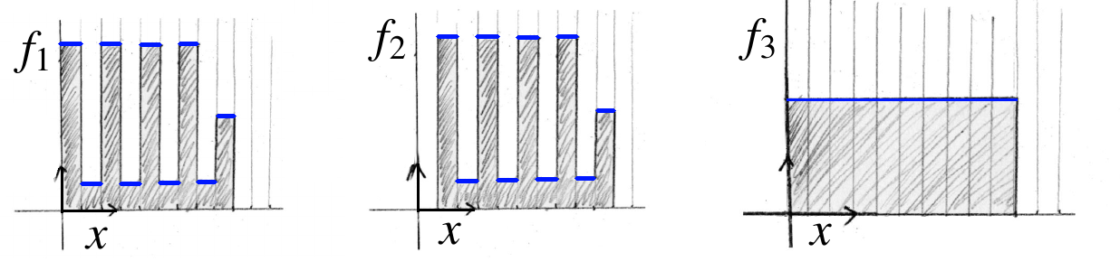
Figure 1: Comparing functions: one would like to say that $f_{1}$ is nearer to $f_{2}$ than $f_{3}$, but the classical $L_{2}$ norm “does not see” that the graph of $f_{2}$ corresponds to the graph of $f_{1}$ slightly shifted along the $x$ axis.

Comparing functions

Consider the functions $f_{1}$, $f_{2}$ and $f_{3}$ in Figure 1. Here we have chosen a function $f_{1}$ with a wildly oscillating graph, and a function $f_{2}$ obtained by translating the graph of $f_{1}$ along the $x$ axis. The function $f_{3}$ corresponds to the mean value of $f_{1}$ (or $f_{2}$). If one measures the relative distances between these functions using the classical $L_{2}$ norm, that is $d_{L_{2}}(f,g)=\int(f(x)-g(x))^{2}dx$, one will find that $f_{1}$ is nearer to $f_{3}$ than $f_{2}$. Optimal transport makes it possible to define a distance that will take into account that the graph of $f_{2}$ can be obtained from $f_{1}$ through a translation (like here), or through a deformation of the graph of $f_{1}$. From the point of view of this new distance, the function $f_{1}$ will be nearer to $f_{2}$ than to $f_{3}$.

Figure 2: Interpolating between two functions: linear interpolation makes a hump disappear while the other hump appears; displacement interpolation, stemming from optimal transport, will displace the hump as expected.

Interpolating between functions:

Now consider the functions $u$ and $v$ in Figure 2. Here we suppose that $u$ corresponds to a certain physical quantity measured at an initial time $t=0$ and that $v$ corresponds to the same phenomenon measured at a final time $t=1$. The problem that we consider now consists in reconstructing what happened between $t=0$ and $t=1$. If we use linear interpolation (Figure 2, top-right), we will see the left hump progressively disappearing while the right hump progressively appears, which is not very realistic if the functions represent for instance a propagating wave. Optimal transport makes it possible to define another type of interpolation (Mc. Cann’s displacement interpolation, Figure 2, bottom-right), that will progressively displace and morph the graph of $u$ into the graph of $v$.

Optimal transport makes it possible to define a geometry of a space of functions, and thus gives a definition of distance in this space, as well as means of interpolating between different functions, and in general, defining the barycenter of a weighted family of functions, in a very general context. Thus, optimal transport appears as a fundamental tool in many applied domains. In computer graphics, applications were proposed, to compare and interpolate objects of diverse natures [BvdPPH11], to generate lenses that can concentrate light to form caustics in a prescribed manner [MMT17, STTP14]. Moreover, optimal transport defines new tools that can be used to discretize Partial Differential Equations, and define new numerical solution mechanisms [BCMO14]. This type of numerical solution mechanism can be used to simulate for instance fluids [GM17], with spectacular applications and results in computer graphics [dGWH⁺15].

The two sections that follow are partly inspired by [Vil09], [San14], [Caf03] and [AG13], but stay at an elementary level. Here the main goal is to give an intuition of the different concepts, and more importantly an idea of the way the relate together. Finally we will see how they can be directly used to design a computational algorithm with very good performance, that can be used in practice in several application domains.

Figure 3: Given two terrains defined by their height functions $u$ and $v$, symbolized here as gray levels, Monge’s problem consists in transforming one terrain into the other one by moving matter through an application $T$. This application needs to satisfy a mass conservation constraint.

2 Monge’s problem

The initial optimal transport problem was first introduced and studied by Monge, right before the French revolution [Mon84]. We first give an intuitive idea of the problem, then quickly introduce the notion of measure, that is necessary to formally state the problem in its most general form and to analyze it.

2.1 Intuition

Monge’s initial motivation to study this problem was very practical: supposing you have an army of workmen, how can you transform a terrain with an initial landscape into a given desired target landscape, while minimizing the total amount of work ?

Monge’s initial problem statement was as follows:

$$\begin{array}[]{l}\inf\limits_{T:X\rightarrow X}\int\limits_{X}c(x,T(x))u(x)dx\\[17.07164pt] \mbox{\ \ \ \ subject to: }\\[17.07164pt] \forall B\subset X,\int\limits_{T^{-1}(B)}u(x)dx=\int\limits_{B}v(x)dx\end{array}$$

where $X$ is a subset of ${\mathbb{R}}^{2}$, $u$ and $v$ are two positive functions defined on $X$ and such that $\int_{X}u(x)dx$ = $\int_{Y}v(x)dx$, and $c(\cdot,\cdot)$ is a convex distance (the Euclidean distance in Monge’s initial problem statement).

The functions $u$ and $v$ represent the height of the current landscape and the height of the target landscape respectively (symbolized as gray levels in Figure 3). The problem consists in finding (if it exists) a function $T$ from $X$ to $X$ that transforms the current landscape $u$ into the desired one $v$, while minimizing the product of the amount of transported earth $u(x)$ with the distance $c(x,T(x))$ to which it was transported. Clearly, the amount of earth is conserved during transport, thus the total quantity of earth should be the same in the source and target landscapes (the integrals of $u$ and $v$ over $X$ should coincide). This global matter conservation constraint needs to be completed with a local one. The local matter conservation constraint enforces that in the target landscape, the quantity of earth received in any subset $B$ of $X$ corresponds to what was transported here, that is the quantity of earth initially present in the pre-image $T^{-1}(B)$ of $B$ under $T$. Without this constraint, one could locally create matter in some places and annihilate matter in other places in a counterbalancing way. A map $T$ that satisfies the local mass conservation constraint is called a transport map.

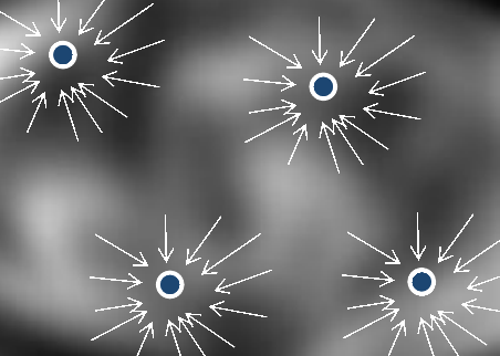
Figure 4: Transport from a function (gray levels) to a discrete point-set (blue disks).

2.2 Monge’s problem with measures

We now suppose that instead of a “target landscape”, we wish to transport earth (or a resource) towards a set of points (that will be denoted by $Y$ for now on), that represent for instance a set of factories that exploit a resource, see Figure 4. Each factory wishes to receive a certain quantity of resource (depending for instance of the number of potential customers around the factory). Thus, the function $v$ that represents the “target landscape” is replaced with a function on a finite set of points. However, if a function $v$ is zero everywhere except on a finite set of points, then its integral over $X$ is also zero. This is a problem, because for instance one cannot properly express the mass conservation constraint. For this reason, the notion of function is not rich enough for representing this configuration. One can use instead measures (more on this below), and associate with each factory a Dirac mass weighted by the quantity of resource to be transported to the factory.

From now on, we will use measures $\mu$ and $\nu$ to represent the “current landscape” and the “target landscape”. These measures are supported by sets $X$ and $Y$, that may be different sets (in the present example, $X$ is a subset of ${\mathbb{R}}^{2}$ and $Y$ is a discrete set of points). Using measures instead of function not only makes it possible to study our “transport to discrete set of factories” problem, but also it can be used to formalize computer objects (meshes) and directly leads to a computational algorithm. This algorithm is very elegant because it is a verbatim computer translation of the mathematical theory (see §7.6). In this particular setting, translating from the mathematical language to the algorithmic setting does not require to make any approximation. This is made possible by the generality of the notion of measure.

The reader who wishes to learn more on measure theory may refer to the textbook [Tao11]. To keep the length of this article reasonable, we will not give here the formal definition of a measure. In our context, one can think of a measure as a “function” that can be only queried using integrals and that can be “concentrated” on very small sets (points). The following table can be used to intuitively translate from the “language of functions” to the “language of measures” :

$$\begin{array}[]{|c|c|}\hline\cr\mbox{Function $u$}&\mbox{Measure $\mu$ }\\[5.69054pt] \hline\cr\int_{B}u(x)dx&\mu(B)\mbox{ or }\int_{B}d\mu\\[5.69054pt] \int_{B}f(x)u(x)dx&\int_{B}f(x)d\mu\\[5.69054pt] u(x)&N/A\\ \hline\cr\end{array}$$

(Note: in contrast with functions, measures cannot be evaluated at a point, they can be only integrated over domains).

In its version with measures, Monge’s problem can be stated as follows:

$$\begin{array}[]{l}\inf\limits_{T:X\rightarrow Y}\int\limits_{X}c(x,T(x))d\mu\ \mbox{ subject to }\ \nu=T\sharp\mu\end{array}$$ (M)

where $X$ and $Y$ are Borel sets (that is, sets that can be measured), $\mu$ and $\nu$ are two measures on $X$ and $Y$ respectively such that $\mu(X)=\nu(Y)$ and $c(\cdot,\cdot)$ is a convex distance. The constraint $\nu=T\sharp\mu$, that reads “$T$ pushes $\mu$ onto $\nu$” corresponds to the local mass conservation constraint. Given a measure $\mu$ on $X$ and a map $T$ from $X$ to $Y$, the measure $T\sharp\mu$ on $Y$, called “the pushforward of $\mu$ by $T$”, is such that $T\sharp\mu(B)=\mu(T^{-1}(B))$ for all Borel set $B\subset Y$. Thus, the local mass conservation constraint means that $\mu(T^{-1}(B))=\nu(B)$ for all Borel set $B$ $\subset$ $Y$.

The local mass conservation constraint makes the problem very difficult: imagine now that you want to implement a computer program that enforces it: the constraint concerns all the subsets $B$ of $Y$. Could you imagine an algorithm that just tests whether a given map satisfies it ? What about enforcing it ? We will see below a series of transformations of the initial problem into equivalent problems, where the constraint becomes linear. We will finally end up with a simple convex optimization problem, that can be solved numerically using classical methods.

Figure 5: A classical example of the existence problem: there is no optimal transport between a segment $L_{1}$ and two parallel segments $L_{2}$ and $L_{3}$ (it is always possible to find a better transport by replacing $h$ with $h/2$).

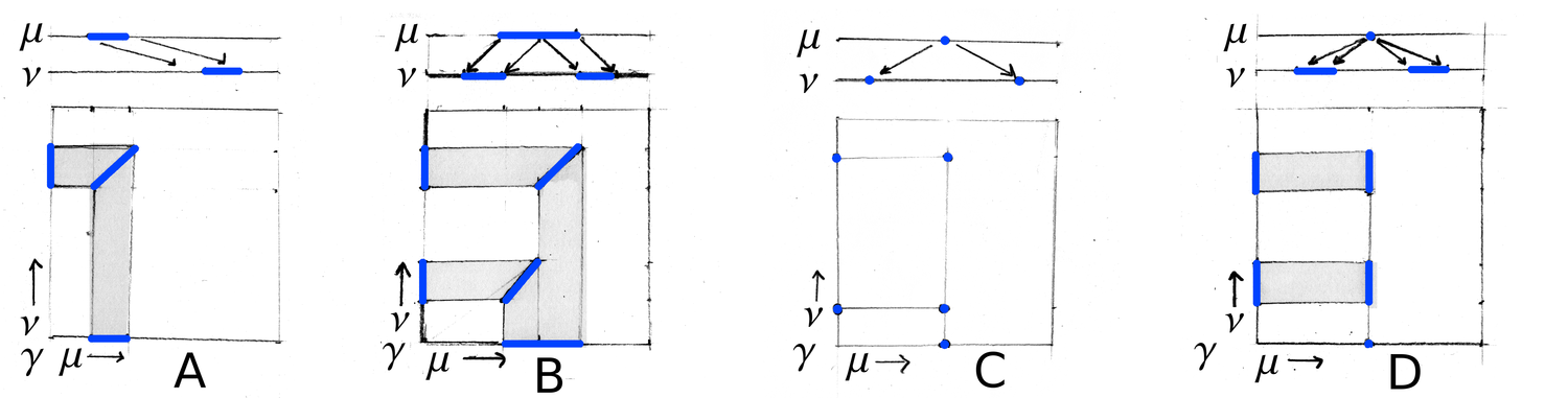
Figure 6: Four example of transport plans in 1D. A: a segment is translated. B: a segment is split into two segments. C: a Dirac mass is split into two Dirac masses; D: a Dirac mass is spread along two segments. The first two examples (A and B) have the form $(Id\times T)\sharp\mu$ where $T$ is a transport map. The third and fourth ones (C and D) have no corresponding transport map, because each of them splits a Dirac mass.

Before then, let us get back to examine the original problem. The local mass conservation constraint is not the only difficulty: the functional optimized by Monge’s problem is non-symmetric, and this causes additional difficulties when studying the existence of solutions for problem (M). The problem is not symmetric because $T$ needs to be a map, therefore the source and target landscape do not play the same role. Thus, it is possible to merge earth (if $T(x_{1})=T(x_{2})$ for two different points $x_{1}$ and $x_{2}$), but it is not possible to split earth (for that, we would need a “map” $T$ that could send the same point $x$ to two different points $y_{1}$ and $y_{2}$). The problem is illustrated in Figure 5: suppose that you want to compute the optimal transport between a segment $L_{1}$ (that symbolizes a “wall of earth”) and two parallel segments $L_{2}$ and $L_{3}$ (that symbolize two “trenches” with a depth that correspond to half the height of the wall of earth). Now we want to transport the wall of earth to the trenches, to make the landscape flat. To do so, it is possible to decompose $L_{1}$ into segments of length $h$, sent alternatively towards $L_{2}$ and $L_{3}$ (Figure 5 on the left). For any length $h$, it is always possible to find a better map $T$, that is a lower value of the functional in (M), by subdividing $L_{1}$ into smaller segments (Figure 5 on the right). The best way to proceed consists in sending from each point of $L_{1}$ half the earth to $L_{2}$ and half the earth to $L_{3}$, which cannot be represented by a map. Thus, the best solution of problem (M) is not a map. In a more general setting, this problem appears each time the source measure $\mu$ has mass concentrated on a manifold of dimension $d-1$ [McC95] (like the segment $L_{1}$ in the present example).

3 Kantorovich’s relaxed problem

To overcome this difficulty, Kantorovich stated a problem with a larger space of solutions, that is, a relaxation of problem (M), where mass can be both split and merged. The idea consists in solving for the “graph of $T$” instead of $T$. One may think of the graph of $T$ as a function $g$ defined on $X\times Y$ that indicates for each couple of points $x\in X,y\in Y$ how much matter goes from $x$ to $y$. However, once again, we cannot use standard functions to represent the graph of $T$: if you think about the graph of a univariate function $x\mapsto f(x)$, it is defined on $\mathbb{R}^{2}$ but concentrated on a curve. For this reason, as in our previous example with factories, one needs to use measures. Thus, we are now looking for a measure $\gamma$ supported by the product space $X\times Y$. The relaxed problem is stated as follows:

$$\begin{array}[]{l}\inf\limits_{\gamma}\left\{\int\limits_{X\times Y}c(x,y)d\gamma\ |\ \gamma\geq 0\mbox{ and }\gamma\in\Pi(\mu,\nu)\right\}\\[14.22636pt] \mbox{where: }\\[8.53581pt] \Pi(\mu,\nu)=\{\gamma\in{\cal P}(X\times Y)\ |\ (P_{X})\sharp\gamma=\mu\ ;\ (P_{Y})\sharp\gamma=\nu\}\end{array}$$ (K)

where $(P_{X})$ and $(P_{Y})$ denote the two projections $(x,y)\in X\times Y\mapsto x$ and $(x,y)\in X\times Y\mapsto y$ respectively.

The two measures $(P_{X})\sharp\gamma$ and $(P_{Y})\sharp\gamma$ obtained by pushing forward $\gamma$ by the two projections are called the marginals of $\gamma$. The measures $\gamma$ in the admissible set $\Pi(\mu,\nu)$, that is, the measures that have $\mu$ and $\nu$ as marginals, are called optimal transport plans. Let us now have a closer look at the two constraints on the marginals $(P_{X})\sharp\gamma=\mu$ and $(P_{X})\sharp\gamma$ that define the set of optimal transport plans $\Pi(\mu,\nu)$. Recalling the definition of the pushforward (previous subsection), these two constraints can also be written as:

$$\begin{array}[]{lcl}(P_{X})\sharp\gamma=\mu&\iff&\forall B\subset X,\int_{B}d\mu=\int_{B\times Y}d\gamma\\[5.69054pt] (P_{Y})\sharp\gamma=\nu&\iff&\forall B^{\prime}\subset Y,\int_{B^{\prime}}d\nu=\int_{X\times B^{\prime}}d\gamma.\end{array}$$ (1)

Intuitively, the first constraint $(P_{X})\sharp\gamma=\mu$ means that everything that comes from a subset $B$ of $X$ should correspond to the amount of matter (initially) contained by $B$ in the source landscape, and the second one $(P_{Y})\sharp\gamma=\nu$ means that everything that goes into a subset $B^{\prime}$ of $Y$ should correspond to the (prescribed) amount of matter contained by $B^{\prime}$ in the target landscape $\nu$.

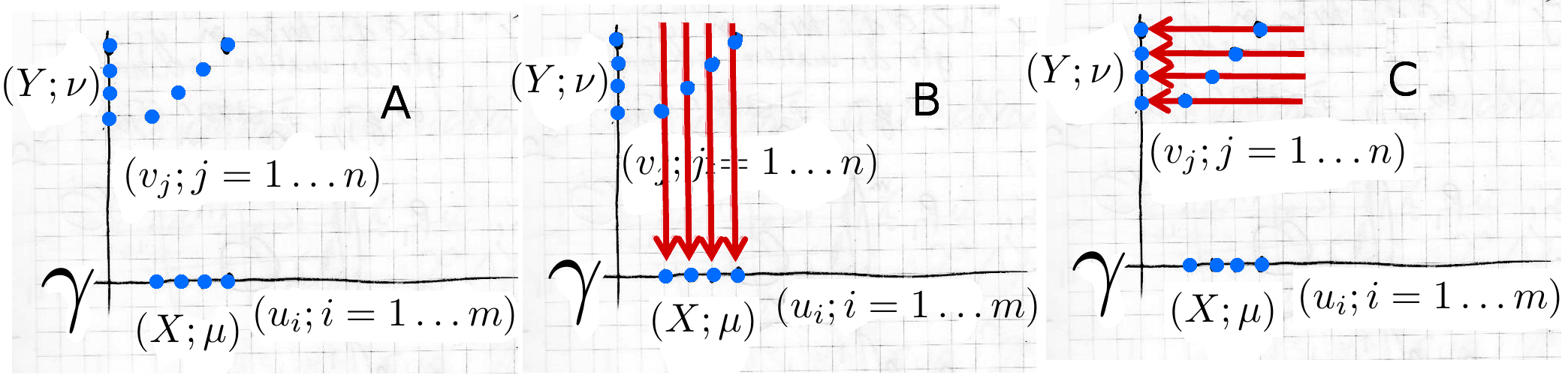
Figure 7: A discrete version of Kantorovich’s problem.

We now examine the relation between the relaxed problem (K) and the initial problem (M). One can easily check that among the optimal transport plans, those with the form $(Id\times T)\sharp\mu$ correspond to a transport map $T$:

Observation 1.

If $(Id\times T)\sharp\mu$ is a transport plan, then $T$ pushes $\mu$ onto $\nu$.

Proof.

$(Id\times T)\sharp\mu$ is in $\Pi(\mu,\nu)$, thus $(P_{Y})\sharp(Id\times T)\sharp\mu=\nu$, or $\left((P_{Y})\circ(Id\times T)\right)\sharp\mu=\nu$, and finally $T\sharp\mu=\nu$. ∎

We can now observe that if a transport plan $\gamma$ has the form $\gamma=(Id\times T)\sharp\mu$, then problem (K) becomes:

$$\mbox{min}\left\{\int\limits_{X\times Y}c(x,y)d\left((Id\times T)\sharp\mu\right)\right\}\quad=\quad\mbox{min}\left\{\int\limits_{X}c(x,T(x))d\mu\right)$$

(one retrieves the initial Monge problem).

To further help grasping an intuition of this notion of transport plan, we show four 1D examples in Figure 6 (the transport plan is then $1D\times 1D=2D$). Intuitively, the transport plan $\gamma$ may be thought of as a “table” indexed by $x$ and $y$ that indicates the quantity of matter transported from $x$ to $y$. More exactly, the measure $\gamma$ is non-zero on subsets of $X\times Y$ that contain points $(x,y)$ such that some matter is transported from $x$ to $y$. Whenever $\gamma$ derives from a transport map $T$, that is if $\gamma$ has the form $(Id\times T)\sharp\mu$, then we can consider $\gamma$ as the “graph of $T$” like in the first two examples of Figure 6 (A) and (B) in Figure 6.

The transport plans of the two other examples (C) and (D) have no associated transport map, because they split Dirac masses. The transport plan associated with Figure 5 has the same nature (but this time in $2D\times 2D=4D$). It cannot be written with the form $(Id\times T)\sharp\mu$ because it splits the mass concentrated in $L_{1}$ into $L_{2}$ and $L_{3}$.

Now the theoretical questions are:

• when does an optimal transport plan exist ?

• when does it admit an associated optimal transport map ?

A standard approach to tackle this type of existence problem is to find a certain regularity both in the functional and in the space of the admissible transport plans, that is, proving that the functional is sufficiently “smooth” and finding a compact set of admissible transport plans. Since the set of admissible transport plans contains at least the product measure $\mu\otimes\nu$, it is non-empty, and existence can be proven thanks to a topological argument that exploits the regularity of the functional and the compactness of the set. Once the existence of a transport plan is established, the other question concerns the existence of an associated transport map. Unfortunately, problem (K) does not directly show the structure required by this reasoning path. However, one can observe that (K) is a linear optimization problem subject to linear constraints. This suggests using certain tools, such as the dual formulation, that was also developed by Kantorovich. With this dual formulation, it is possible to exhibit an interesting structure of the problem, that can be used to answer both questions (existence of a transport plan, and existence of an associated transport map).

4 Kantorovich’s dual problem

Kantorovich’s duality applies to problem (K), in its most general form (with measures). To facilitate understanding, we will consider instead a discrete version of problem (K), where the involved entities are vectors and matrices (instead of measures and operators). This makes it easy to better discern the structure of (K), that is the linear nature of both the functional and the constraints. This also makes it easier for the reader to understand how to construct the dual by manipulating simpler objects (matrices and vectors), however the structure of the reasoning is the same in the general case.

4.1 The discrete Kantorovich problem

In Figure 7, we show a discrete version of the 1D transport between two segments of Figure 6. The measures $\mu$ and $\nu$ are replaced with vectors $U=(u_{i})_{i=1\ldots m}$ and $V=(v_{j})_{i=1\ldots n}$. The transport plan $\gamma$ becomes a set of coefficients $\gamma_{ij}$. Each coefficient $\gamma_{ij}$ indicates the quantity of matter that will be transported from $u_{i}$ to $v_{j}$. The discrete Kantorovich problem can be written as follows:

$$\quad\quad\min\limits_{\gamma}<C,\gamma>\mbox{ subject to }\left\{\begin{array}[]{l}{\bf P_{x}}\gamma=U\\ {\bf P_{y}}\gamma=V\\ \gamma_{i,j}\geq 0\quad\forall i,j\end{array}\right.$$ (2)

where $\gamma$ is the vector of $\mathbb{R}^{m\times n}$ with all coefficients $\gamma_{ij}$ (that is, the matrix $\gamma_{ij}$ “unrolled” into a vector), and $C$ the vector of $\mathbb{R}^{m\times n}$ with the coefficients $c_{ij}$ indicating the transport cost between point $i$ and point $j$ (for instance, the Euclidean cost). The objective function is simply the dot product, denoted by $<C,\gamma>$, of the cost vector $C$ and the vector $\gamma$. The objective function is linear in $\gamma$. The constraints on the marginals (1) impose in this discrete version that the sums of the $\gamma_{ij}$ coefficients over the columns correspond to the $u_{i}$ coefficients (Figure 7-B) and the sums over the rows correspond to the $v_{j}$ coefficients (Figure 7-C). Intuitively, everything that leaves point $i$ should correspond to $u_{i}$, that is the quantity of matter initially present in $i$ in the source landscape, and everything that arrives at a point $j$ should correspond to $v_{j}$, that is the quantity of matter desired at $j$ in the target landscape. As one can easily notice, in this form, both constraints are linear in $\gamma$. They can be written with two matrices ${\bf P_{x}}$ and ${\bf P_{y}}$, of dimensions $m\times mn$ and $n\times mn$ respectively.

4.2 Constructing the Kantorovich dual in the discrete setting

We introduce, arbitrarily for now, the following function $L$ defined by:

$$L(\varphi,\psi)=<C,\gamma>-<\varphi,{\bf P_{x}}\gamma-U>-<\psi,{\bf P_{y}}\gamma-V>$$

that takes as arguments two vectors, $\varphi$ in ${\mathbb{R}}^{m}$ and $\psi$ in ${\mathbb{R}}^{n}$. The function $L$ is constructed from the objective function $<C,\gamma>$ from which we subtracted the dot products of $\varphi$ and $\psi$ with the vectors that correspond to the degree of violation of the constraints. One can observe that:

$$\begin{array}[]{lcl}\sup\limits_{\varphi,\psi}[L(\varphi,\psi)]&=&<C,\gamma>\mbox{ if }{\bf P_{x}}\gamma=U\mbox{ and }{\bf P_{y}}\gamma=V\\ &=&+\infty\mbox{ otherwise.}\end{array}$$

Indeed, if for instance a component $i$ of ${\bf P_{x}}\gamma$ is non-zero, one can make $L$ arbitrarily large by suitably choosing the associated coefficient $\varphi_{i}$.

Now we consider:

$$\inf\limits_{\gamma\geq 0}\left[\sup\limits_{\varphi,\psi}[L(\varphi,\psi)]\right]=\inf\limits_{\tiny\begin{array}[]{l}\gamma\geq 0\\ {\bf P_{x}}\gamma=U\\ {\bf P_{y}}\gamma=V\end{array}}\left[<C,\gamma>\right].$$

There is equality, because to minimize $\sup[L(\varphi,\psi)]$, $\gamma$ has no other choice than satisfying the constraints (see the previous observation). Thus, we obtain a new expression (left-hand side) of the discrete Kantorovich problem (right-hand side). We now further examine it, and replace $L$ by its expression:

$$\inf\limits_{\gamma\geq 0}\left[\sup\limits_{\varphi,\psi}\left(\begin{array}[]{ll}<C,\gamma>&-<\varphi,{\bf P_{x}}\gamma-U>\\ &-<\psi,{\bf P_{y}}\gamma-V>\end{array}\right)\right]$$ (5)

$$= \sup\limits_{\varphi,\psi}\left[\inf\limits_{\gamma\geq 0}\left(\begin{array}[]{ll}<C,\gamma>&-<\varphi,{\bf P_{x}}\gamma-U>\\ &-<\psi,{\bf P_{y}}\gamma-V>\end{array}\right)\right]$$ (8)

$$= \sup\limits_{\varphi,\psi}\left[\inf\limits_{\gamma\geq 0}\left(\begin{array}[]{l}<\gamma,C-{\bf P_{x}}^{t}\varphi-{\bf P_{y}}^{t}\psi>+\\[2.84526pt] <\varphi,U>+<\psi,V>\end{array}\right)\right]$$ (11)

$$= \sup\limits_{\tiny\begin{array}[]{c}\varphi,\psi\\ {\bf P_{x}}^{t}\varphi+{\bf P_{y}}^{t}\psi\leq C\end{array}}\left[<\varphi,U>+<\psi,V>\right].\quad\quad$$ (14)

The first step (8) consists in exchanging the “$\inf$” and “$\sup$”. Then we rearrange the terms (11). By reinterpreting this equation as a constrained optimization problem (similarly to what we did in the previous paragraph), we finally obtain the constrained optimization problem in (14). In the constraint ${\bf P_{x}}^{t}\varphi+{\bf P_{y}}^{t}\psi\leq C$, the inequality is to be considered componentwise. Finally, the problem (14) can be rewritten as:

$$\begin{array}[]{l}\sup\limits_{\varphi,\psi}\left[<\varphi,U>+<\psi,V>\right]\\[5.69054pt] \mbox{ subject to }\varphi_{i}+\psi_{j}\leq c_{ij},\quad\forall i,j.\end{array}$$ (15)

As compared to the primal problem (2) that depends on $m\times n$ variables (all the coefficients $\gamma_{ij}$ of the optimal transport plan for all couples of points $(i,j)$), this dual problem depends on $m+n$ variables (the components $\varphi_{i}$ and $\psi_{j}$ attached to the source points and target points). We will see later how to further reduce the number of variables, but before then, we go back to the general continuous setting (that is, with functions, measures and operators).

4.3 The Kantorovich dual in the continuous setting

The same reasoning path can be applied to the continuous Kantorovich problem (K), leading to the following problem (DK):

$$\begin{array}[]{l}(DK)\quad\quad\sup\limits_{\varphi,\psi}\left[\int\limits_{X}\varphi d\mu+\int\limits_{Y}\psi d\nu\right]\\[11.38109pt] \mbox{ subject to: }\\ \varphi(x)+\psi(y)\leq c(x,y)\quad\forall(x,y)\in X\times Y,\end{array}$$ (16)

where $\varphi$ and $\psi$ are now functions defined on $X$ and $Y$.

The classical image that gives an intuitive meaning to this dual problem is to consider that instead of transporting earth by ourselves, we are now hiring a company that will do the work on our behalf. The company has a special way of determining the price: the function $\varphi(x)$ corresponds to what they charge for loading earth at $x$, and $\psi(y)$ corresponds to what they charge for unloading earth at $y$. The company aims at maximizing its profit (this is why the dual problem is a “sup” rather than an “inf)”, but it cannot charge more than what it would cost us if we were doing the work by ourselves (hence the constraint).

The existence of solutions for (DK) remains difficult to study, because the set of functions $\varphi,\psi$ that satisfy the constraint is not compact. However, it is possible to reveal more structure of the problem, by introducing the notion of c-transform, that makes it possible to exhibit a set of admissible functions with sufficient regularity:

Definition 1.

• For $f$ any function on $Y$ with values in $\mathbb{R}\cup\{-\infty\}$ and not identically $-\infty$, we define its $c$-transform by

  $$f^{c}(x)=\inf\limits_{y\in Y}\left[c(x,y)-f(y)\right],\quad x\in X.$$

• If a function $\varphi$ is such that there exists a function $f$ such that $\varphi=f^{c}$, then $\varphi$ is said to be $c$-concave;

• ${\bf\Psi}_{c}(X)$ denotes the set of c-concave functions on $X$.

We now show two properties of (DK) that will allow us to restrict the problem to the class of $c$-concave functions to search for $\varphi$ and $\psi$:

Observation 2.

If the pair $(\varphi,\psi)$ is admissible for (DK), then the pair $(\psi^{c},\psi)$ is admissible as well.

Proof.

$$\begin{array}[]{l}\left\{\begin{array}[]{l}\forall(x,y)\in X\times Y,\varphi(x)+\psi(y)\leq c(x,y)\\ \psi^{c}(x)=\inf\limits_{y\in Y}\left[c(x,y)-\psi(y)\right]\end{array}\right.\\[8.53581pt] \begin{array}[]{lcl}\psi^{c}(x)+\psi(y)&=&\inf\limits_{y^{\prime}\in Y}\left[c(x,y^{\prime})-\psi(y^{\prime})\right]+\psi(y)\\ &\leq&(c(x,y)-\psi(y))+\psi(y)\\ &\leq&c(x,y).\end{array}\end{array}$$

∎

Observation 3.

If the pair $(\varphi,\psi)$ is admissible for (DK), then one obtains a better pair by replacing $\varphi$ with $\psi^{c}$:

Proof.

$$\left.\begin{array}[]{lcl}&\psi^{c}(x)=&\inf\limits_{y\in Y}\left[c(x,y)-\psi(y)\right]\\ \forall y\in Y,&\varphi(x)\leq&c(x,y)-\psi(y)\end{array}\right\}\Rightarrow\psi^{c}(x)\leq\varphi(x).$$

∎

In terms of the previous intuitive image, this means that by replacing $\varphi$ with $\psi^{c}$, the company can charge more while the price remains acceptable for the client (that is, the constraint is satisfied). Thus, we have:

$$\begin{array}[]{ll}\inf(K)&=\sup\limits_{\varphi\in{\bf\Psi}_{c}(X)}\quad\int\limits_{X}\varphi\ d\mu+\int\limits_{Y}\varphi^{c}\ d\nu\\[11.38109pt] &=\sup\limits_{\psi\in{\bf\Psi}_{c}(Y)}\quad\int\limits_{X}\psi^{c}\ d\mu+\int\limits_{Y}\psi\ d\nu\end{array}$$

We do not give here the detailed proof for existence. The reader is referred to [Vil09], Chapter 4. The idea is that we are now in a much better situation, since the set of admissible functions ${\bf\Psi}_{c}(X)$ is compact.

The optimal value gives an interesting information, that is the minimum cost of transforming $\mu$ into $\nu$. This can be used to define a distance between distributions, and also gives a way to compare different distributions, which is of practical interest for some applications.

5 From the Kantorovich dual to the optimal transport map

5.1 The $c$-superdifferential

Suppose now that in addition to the optimal cost you want to know the associated way to transform $\mu$ into $\nu$, in other words, when it exists, the map $T$ from $X$ to $Y$ which associated transport plan $(Id\times T)\sharp\mu$ minimizes the functional of the Monge problem. A result characterizes the support of $\gamma$, that is the subset $\partial^{c}\varphi\subset X\times Y$ of the pairs of points $(x,y)$ connected by the transport plan:

Theorem 1.

Let $\varphi$ a $c$-concave function. For all $(x,y)\in\partial^{c}\varphi$, we have

$$\nabla\varphi(x)-\nabla_{x}c(x,y)=0,$$

where $\partial^{c}\varphi=\{(x,y)\ |\ \varphi(z)\leq\varphi(x)+(c(z,y)-c(x,y)),\forall z\in X\}$ denotes the so-called $c$-superdifferential of $\varphi$.

Proof.

See [Vil09] chapters 9 and 10. ∎

In order to give an idea of the relation between the $c$-superdifferential and the associated transport map $T$, we present below a heuristic argument: consider a point $(x,y)$ in the $c$-superdifferential $\partial^{c}\varphi$, then for all $z\in X$ we have

$$c(x,y)-\varphi(x)\leq c(z,y)-\varphi(z).$$ (17)

Now, by using (17), we can compute the derivative at $x$ with respect to an arbitrary direction $w$

$$\lim_{t\to 0^{+}}\frac{\varphi(x+tw)-\varphi(x)}{t}\leq\lim_{t\to 0^{+}}\frac{c(x+tw,y)-c(x,y)}{t}$$

and we obtain $\nabla\varphi(x)\cdot w\leq\nabla_{x}c(x,y)\cdot w$. We can do the same derivation along direction $-w$ instead of $w$, and then we get $\nabla\varphi(x)\cdot w=\nabla_{x}c(x,y)\cdot w$, $\forall w\in X$.

In the particular case of the $L_{2}$ cost, that is with $c(x,y)=1/2\|x-y\|^{2}$, this relation becomes $\forall(x,y)\in\partial^{c}\varphi,\nabla\varphi(x)+y-x=0$, thus, when the optimal transport map $T$ exists, it is given by

$$T(x)=x-\nabla\varphi(x)=\nabla(\|x\|^{2}/2-\varphi(x)).$$

Not only this gives an expression of $T$ in function of $\varphi$, which is of high interest to us if we want to compute the transport explicitly. In addition, this makes it possible to characterize $T$ as the gradient of a convex function (see also Brenier’s polar factorization theorem [Bre91]). This convexity property is interesting, because it means that two “transported particles” $x_{1}\mapsto T(x_{1})$ et $x_{2}\mapsto T(x_{2})$ will never collide. We now see how to prove these two assertions ($T$ gradient of a convex function and absence of collision) in the case of the $L_{2}$ transport (with $(c(x,y)=1/2\|x-y\|^{2}$).

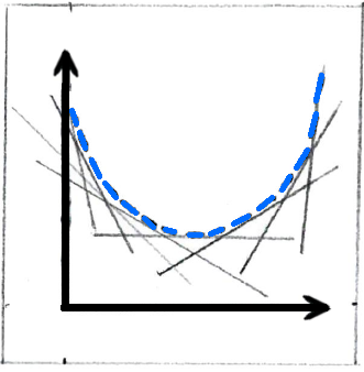
Figure 8: The upper envelope of a family of affine functions is a convex function.

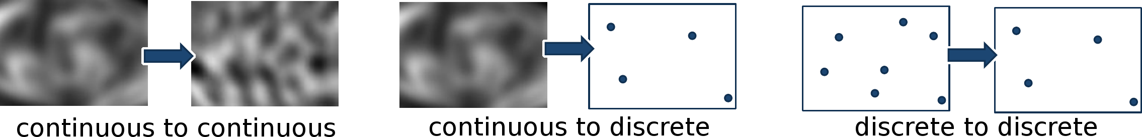
Figure 9: Different types of transport, with continuous and discrete measures $\mu$ and $\nu$.

Observation 4.

If $c(x,y)$ = $1/2\|x-y\|^{2}$ and $\varphi\in{\bf\Psi}_{c}(X)$, then $\bar{\varphi}:x\mapsto\bar{\varphi}(x)=\|x\|^{2}/2-\varphi(x)$ is a convex function (it is an equivalence if $X=Y=\mathbb{R}^{d}$, see [San15]).

Proof.

$$\begin{split}\varphi(x)=&\psi^{c}(x)\\ =&\inf\limits_{y}\left[\frac{\|x-y\|^{2}}{2}-\psi(y)\right]\\ =&\inf\limits_{y}\left[\frac{\|x\|^{2}}{2}-x\cdot y+\frac{\|y\|^{2}}{2}-\psi(y)\right].\end{split}$$

Then,

$$\begin{split}-\bar{\varphi}(x)=&\varphi(x)-\frac{\|x\|^{2}}{2}=\inf\limits_{y}\left[-x\cdot y+\left(\frac{\|y\|^{2}}{2}-\psi(y)\right)\right].\end{split}$$

Or equivalently,

$$\begin{split}\bar{\varphi}(x)=&\sup\limits_{y}\left[x\cdot y-\left(\frac{\|y\|^{2}}{2}-\psi(y)\right)\right].\end{split}$$

The function $x\mapsto x\cdot y-\left(\frac{\|y\|^{2}}{2}-\psi(y)\right)$ is affine in $x$, therefore the graph of $\bar{\varphi}$ is the upper envelope of a family of hyperplanes, therefore $\bar{\varphi}$ is a convex function (see Figure 8). ∎

Observation 5.

We now consider the trajectories of two particles parameterized by $t\in[0,1]$, $t\mapsto(1-t)x_{1}+tT(x_{1})$ and $t\mapsto(1-t)x_{2}+tT(x_{2})$. If $x_{1}\neq x_{2}$ and $0<t<1$ then there is no collision between the two particles.

Proof.

By contradiction, suppose there is a collision, that is there exists $t\in(0,1)$ and $x_{1}\neq x_{2}$ such that

$$(1-t)x_{1}+tT(x_{1})=(1-t)x_{2}+tT(x_{2}).$$

Since $T=\nabla\bar{\varphi}$, we can rewrite the last equality as

$$(1-t)(x_{1}-x_{2})+t(\nabla\bar{\varphi}(x_{1})-\nabla\bar{\varphi}(x_{2}))=0.$$

Therefore,

$$(1-t)\|x_{1}-x_{2}\|^{2}+t(\nabla\bar{\varphi}(x_{1})-\nabla\bar{\varphi}(x_{2}))\cdot(x_{1}-x_{2})=0.$$

The last step leads to a contradiction, between the left-hand side is the sum of two strictly positive numbers (recalling the definition of the convexity of $\bar{\varphi}$: $\forall x_{1}\neq x_{2},(x_{1}-x_{2})\cdot(\nabla\bar{\varphi}(x_{1})-\nabla\bar{\varphi}(x_{2}))>0$ ) ∎

6 Continuous, discrete and semi-discrete transport

The properties that we have presented in the previous sections are true for any couple of source and target measures $\mu$ and $\nu$, that can derive from continuous functions or that can be discrete empirical measures (sum of Dirac masses). Figure 9 presents three configurations that are interesting to study. These configurations have specific properties, that lead to different algorithms for computing the transport. We give here some indications and references concerning the continuous $\rightarrow$ continuous and discrete $\rightarrow$ discrete cases. Then we will develop the continuous $\rightarrow$ discrete case with more details in the next section.

6.1 The continuous $\rightarrow$ continuous case and Monge-Ampère equation

We recall that when the optimal transport map exists, in the case of the $L_{2}$ cost (that is, $c(x,y)=1/2\|x-y\|^{2}$), it can be deduced from the function $\varphi$ by using the relation $T(x)=\nabla\bar{\varphi}=x-\nabla\varphi$. The change of variable formula for integration over a subset $B$ of $X$ can be written as:

$$\forall B\subset X,\int_{B}1d\mu=\mu(B)=\nu(T(B))=\int_{B}\left|\det J_{T}(x)\right|d\mu$$ (18)

where $J_{T}$ denotes the Jacobian matrix of $T$ and $\det$ denotes the determinant.

If $\mu$ and $\nu$ have densities $u$ and $v$ respectively, that is $\forall B,\mu(B)=\int_{B}u(x)dx$ and $\nu(B)=\int_{B}v(x)dx$, then one can (formally) consider (18) pointwise in $X$:

$$\forall x\in X,\ u(x)=\left|\det J_{T}(x)\right|v(T(x)).$$ (19)

By injecting $T=\nabla\bar{\varphi}$ and $J_{T}=H\bar{\varphi}$ into (19), one obtains:

$$\forall x\in X,\ u(x)=\left|\det H\bar{\varphi}(x)\right|v(\nabla\bar{\varphi}(x)),$$ (20)

where $H\bar{\varphi}$ denotes the Hessian matrix of $\bar{\varphi}$. Equation (20) is known ad the Monge-Ampère equation. It is a highly non-linear equation, and its solutions when they exist often present singularities. Note that the derivation above is purely formal, and that studying the solutions of the Monge-Ampère equation require using more sophisticated tools. In particular, it is possible to define several types of weak solutions (viscosity solutions, solution in the sense of Brenier, solutions in the sense of Alexandrov …). Several algorithms to compute numerical solutions of the Monge-Ampère equations were proposed. As such, see for instance the Benamou-Brenier algorithm [BB00], that uses a dynamic formulation inspired by fluid dynamics (incompressible Euler equation with specific boundary conditions). See also [PPO14].

6.2 The discrete $\rightarrow$ discrete case

If $\mu$ is the sum of $m$ Dirac masses and $\nu$ the sum of $n$ Dirac masses, then the problem boils down to finding the $m\times n$ coefficients $\gamma_{ij}$ that give for each pair of points $i$ of the source space and $j$ of the target space the quantity of matter transported from $i$ to $j$. This corresponds to the transport plan in the discrete Kantorovich problem that we have seen previously §4. This type of problem (referred to as an assignment problem) can be solved by different methods of linear programming [BDM09]. These method can be dramatically accelerated by adding a regularization term, that can be interpreted as the entropy of the transport plan [Leo13]. This regularized version of optimal transport can be solved by highly efficient numerical algorithms [Cut13].

6.3 The continuous $\rightarrow$ discrete case

This configuration, also called semi-discrete, corresponds to a continuous function transported to a sum of Dirac masses (see the examples of c-concave functions in [GM96]). This correspond to our example with factories that consume a resource, in §2.2. Semi-discrete transport has interesting connections with some notions of computational geometry and some specific sets of convex polyhedra that were studied by Alexandrov [Ale05] and later by Aurenhammer, Hoffman and Aranov [AHA92]. The next section is devoted to this configuration.

7 Semi-discrete transport

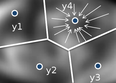
Figure 10: Semi-discrete transport: gray levels symbolize the quantity of a resource that will be transported to 4 factories. Each factory will be allocated a part of the terrain in function of the quantity of resource that it should collect.

We now suppose that the source measure $\mu$ is continuous, and that the target measure $\nu$ is a sum of Dirac masses. A practical example of this type of configuration corresponds to a resource which available quantity is represented by a function $u$. The resource is collected by a set of $n$ factories, as shown in Figure 10. Each factory is supposed to collect a certain prescribed quantity of resource $\nu_{j}$. Clearly, the sum of all prescriptions corresponds to the total quantity of available resource ($\sum_{j=1}^{n}\nu_{j}=\int_{X}u(x)dx$).

7.1 Semi-discrete Monge problem

In this specific configuration, the Monge problem becomes:

$$\begin{array}[]{l}\inf\limits_{T:X\rightarrow Y}\int\limits_{X}c(x,T(x))u(x)dx,\mbox{ subject to}\int\limits_{T^{-1}(y_{j})}u(x)dx=\nu_{j},\forall j.\end{array}$$

A transport map $T$ associates with each point $x$ of $X$ one of the points $y_{j}$. Thus, it is possible to partition $X$, by associating to each $y_{j}$ the region $T^{-1}(y_{j})$ that contains all the points transported towards $y_{j}$ by $T$. The constraint imposes that the quantity of collected resource over each region $T^{-1}(y_{j})$ corresponds to the prescribed quantity $\nu_{j}$.

Let us now examine the form of the dual Kantorovich problem. In terms of measure, the source measure $\mu$ has a density $u$, and the target measure $\nu$ is a sum of Dirac masses $\nu=\sum_{j=1}^{n}\nu_{j}\delta_{y_{j}}$, supported by the set of points $Y=\left\{y_{j}\right\}$. We recall that in its general form, the dual Kantorovich problem is written as follows:

$$\sup\limits_{\psi\in{\bf\Psi^{c}}(Y)}\left[\int_{X}\psi^{c}(x)d\mu+\int_{Y}\psi(y)d\nu\right].$$ (21)

In our semi-discrete case, the functional becomes a function of $n$ variables, with the following form:

$$F(\psi) = \!F(\psi_{1},\psi_{2},\ldots\psi_{n})$$ (22)

$$= \!\int\limits_{X}\!\psi^{c}(x)u(x)dx+\sum_{j=1}^{n}\psi_{j}\nu_{j}$$ (23)

$$= \!\int\limits_{X}\!\inf\limits_{y_{j}\in Y}\left[c(x,y_{j})-\psi_{j}\right]u(x)dx+\sum_{j=1}^{n}\psi_{j}\nu_{j}$$ (24)

$$= \!\sum\limits_{j=1}^{n}\int\limits_{\mathrm{L}ag_{\psi}^{c}(y_{j})}\!\left(c(x,y_{j})-\psi_{j}\right)u(x)dx+\sum_{j=1}^{n}\psi_{j}\nu_{j}.$$ (25)

The first step (23) takes into account the nature of the measures $\mu$ and $\nu$. In particular, one can notice that the measure $\nu$ is completely defined by the scalars $\nu_{j}$ associated with the points $y_{j}$, and the function $\psi$ is defined by the scalars $\psi_{j}$ that correspond to its value at each point $y_{j}$. The integral $\int_{Y}\psi(y)d\nu$ becomes the dot product $\sum_{j}\psi_{j}\nu_{j}$. Thus, the functional that corresponds to the dual Kantorovich problem becomes a function $F$ that depends on $n$ variables (the $\psi_{j}$). Let us now replace the c-conjugate $\psi^{c}$ with its expression, which gives (24). The integral in the left term can be reorganized, by grouping the points of $X$ for which the same point $y_{j}$ minimizes $c(x,y_{j})-\psi_{j}$, which gives (25), where the Laguerre cell $\mathrm{L}ag_{\psi}^{c}(y_{j})$ is defined by:

$$\mathrm{L}ag_{\psi}^{c}(y_{j})=\left\{x\in X\quad|\quad c(x,y_{j})-\psi_{j}\leq c(x,y_{k})-\psi_{k},\ \forall k\neq j\right\}.$$

The Laguerre diagram, formed by the union of the Laguerre cells, is a classical structure in computational geometry. In the case of the $L_{2}$ cost $c(x,y)=1/2\|x-y\|^{2}$, it corresponds to the power diagram, that was studied by Aurenhammer at the end of the 80’s [Aur87]. One of its particularities is that the boundaries of the cells are rectilinear, making it reasonably easy to design computational algorithms to construct them.

     

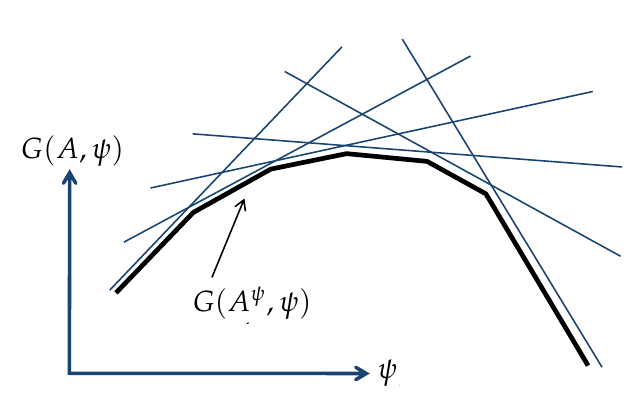
Figure 11: The objective function of the dual Kantorovich problem is concave, because its graph is the lower envelope of a family of affine functions.

7.2 Concavity of $F$

The objective function $F$ is a particular case of the Kantorovich dual, and naturally inherits its properties, such as its concavity (that we did not discuss yet). This property is interesting both from a theoretical point of view, to study the existence and uniqueness of solutions, and from a practical point of view, to design efficient numerical solution mechanisms. In the semi-discrete case, the concavity of $F$ is easier to prove than in the general case. We summarize here the proof by Aurenhammer et. al [AHA92], that leads to an efficient algorithm [Mér11], [Lév15], [KMT16].

Theorem 2.

The objective function $F$ of the semi-discrete Kantorovich dual problem (21) is concave.

Proof.

Consider the function $G$ defined by:

$$G(A,\left[\psi_{1},\ldots\psi_{n}\right])=\int\limits_{X}\left(c(x,y_{A(x)})-\psi_{A(x)}\right)u(x)dx,$$ (26)

and parameterized by an assignment $A~{}:X\rightarrow[1\ldots n]$, that is, a function that associates with each point $x$ of $X$ the index $j$ of one of the points $y_{j}$. If we denote $A^{-1}(j)=\left\{x|A(x)=j\right\}$, then $G$ can be also written as:

$$\begin{array}[]{lcl}G(A,\psi)&=&\sum\limits_{j}\int\limits_{A^{-1}(j)}\left(c(x,y_{j})-\psi_{j}\right)u(x)dx\\[5.69054pt] &=&\sum\limits_{j}\int\limits_{A^{-1}(j)}c(x,y_{j})u(x)dx-\sum\limits_{j}\psi_{j}\int\limits_{A^{-1}(j)}u(x)dx.\end{array}$$ (27)

The first term does not depend on the $\psi_{j}$, and the second one is a linear combination of the $\psi_{j}$ coefficients, thus, for a given fixed assignment $A$, $\psi\mapsto G(A,\psi)$ is an affine function of $\psi$. Figure 11 depicts the appearance of the graph of $G$ for different assignment. The horizontal axis symbolizes the components of the vector $\psi$ (of dimension $n$) and the vertical axis the value of $G(A,\psi)$. For a given assignment $A$, the graph of $G$ is an hyperplane (symbolized here by a straight line).

Among all the possible assignments $A$, we distinguish $A^{\psi}$ that associates with a point $x$ the index $j$ of the Laguerre cell $x$ belongs to , that is:

$$A^{\psi}(x)=\arg\min\limits_{j}\left[c(x,y_{j})-\psi_{j}\right].$$

For a fixed vector $\psi=\psi^{0}$, among all the possible assignments $A$, the assignment $A^{\psi^{0}}$ minimizes the value $G(A,\psi^{0})$, because it minimizes the integrand pointwise (see Figure 11 on the left. Thus, since $G$ is affine with respect to $\psi$, the graph of the function $\psi\rightarrow G(A^{\psi},\psi)$ is the lower envelope of a family of hyperplanes (symbolized as straight lines in Figure 11 on the right), hence $\psi\rightarrow G(A^{\psi},\psi)$ is a concave function. Finally, the objective function $F$ of the dual Kantorovich problem can be written as $F(\psi)=G(A^{\psi},\psi)+\sum_{j}\nu_{j}\psi_{j}$, that is, the sum of a concave function and a linear function, hence it is also a concave function. ∎

7.3 The semi-discrete optimal transport map

Let us now examine the $c$-superdifferential $\partial^{c}\psi$, that is, the set of points ($x\in X$, $y\in Y$) connected by the optimal transport map. We recall that the $c$-superdifferential $\partial^{c}\psi$ can be defined alternatively as $\partial^{c}\psi=\left\{(x,y_{j})\ |\ \psi^{c}(x)+\psi_{j}=c(x,y_{j})\right\}$. Consider a point $x$ of $X$ that belongs to the Laguerre cell $\mathrm{L}ag_{\psi}^{c}(y_{j})$. The $c$-superdifferential $[\partial^{c}\psi](x)$ at $x$ is defined by:

$$[\partial^{c}\psi](x) = \left\{y_{k}\ |\ \psi^{c}(x)+\psi_{k}=c(x,y_{k})\right\}$$ (28)

$$= \left\{y_{k}\ |\ \inf_{y_{l}}\left[c(x,y_{l})-\psi_{l}\right]+\psi_{k}=c(x,y_{k})\right\}$$ (29)

$$= \left\{y_{k}\ |\ c(x,y_{j})-\psi_{j}+\psi_{k}=c(x,y_{k})\right\}$$ (30)

$$= \left\{y_{k}\ |\ c(x,y_{j})-\psi_{j}=c(x,y_{k})-\psi_{k}\right\}$$ (31)

$$= \left\{y_{j}\right\}.$$ (32)

In the first step (29), we replace $\psi^{c}$ by its definition, then we use the fact that $x$ belongs to the Laguerre cell of $y_{j}$ (30), and finally, the only point of $Y$ that satisfies (31) is $y_{j}$ because we have supposed $x$ inside the Laguerre cell of $y_{j}$.

To summarize, the optimal transport map $T$ moves each point $x$ to the point $y_{j}$ associated with the Laguerre cell $\mathrm{L}ag_{\psi}^{c}(y_{j})$ that contains $x$. The vector $\psi_{1},\ldots\psi_{n}$ is the unique vector that maximizes the discrete dual Kantorovich function $F$ such that $\psi$ is c-concave. It is possible to show that $\psi$ is c-concave if and only if no Laguerre cell is empty of matter, that is the integral of $u$ is non-zero on each Laguerre cell. Indeed, we have the following results:

Theorem 3.

Let $Y=\{y_{1},\ldots,y_{n}\}$ be a set of $n$ points. Let $\psi$ be any function defined on $Y$ such that $\mathrm{L}ag_{\psi}^{c}(y_{i})$ are not empty sets. Then $\psi$ is a $c$-concave function.

Proof.

By definition, for $i=1,2,\ldots,k$

$$\begin{split}(\psi^{c})^{c}(y_{i})&=\inf\limits_{x\in X}\left[c(x,y_{i})-\psi^{c}(x)\right]\\ &=\inf\limits_{x\in X}\left[c(x,y_{i})-\left(\inf\limits_{y_{j}\in Y}\left[c(x,y_{j})-\psi(y_{j})\right]\right)\right]\\ &=\inf\limits_{x\in X}\left\{\begin{array}[]{ll}\psi(y_{i}),\quad\quad\quad\quad\quad\ \quad\quad\quad\quad\hbox{if $x\in\mathrm{L}ag_{\psi}^{c}(y_{i})$ }\\ c(x,y_{i})-(\overbrace{c(x,y_{j})-\psi(y_{j})}^{\quad<(c(x,y_{i})-\psi(y_{i}))}),\ \hbox{if $x\in\mathrm{L}ag_{\psi}^{c}(y_{j})$ $(j\neq i)$ }\end{array}\right.\\ &=\psi(y_{i}).\end{split}$$

This allows to conclude that $\psi$ is a $c$-convex function (see [San15, Proposition 1.34]). ∎

Moreover, the converse of the theorem is also true:

Theorem 4.

Let $Y=\{y_{1},\ldots,y_{n}\}$ be a set of $n$ points. Let $\psi$ be a $c$-concave function defined on $Y$. Then the sets $\mathrm{L}ag_{\psi}^{c}(y_{i})$ are not empty for all $i=1,\ldots,n$,.

Proof.

Reasoning by contradiction, we suppose that $\psi$ is a $c$-concave function and there exist $i_{0}\in\{1,\ldots,n\}$ such that $\mathrm{L}ag_{\psi}^{c}(y_{i_{0}})=\emptyset$. Then, from definition

$$\begin{split}\forall x\in X,\ \exists j\in\{1,\ldots,n\}\ \hbox{with}\ j\neq i_{0},\ \hbox{and}\ \epsilon_{j}>0\ \hbox{such that}\\ c(x,y_{i_{0}})-\psi(y_{i_{0}})\geq c(x,y_{j})-\psi(y_{j})+\epsilon_{j}.\end{split}$$

We will write $x=x_{j}$. Thus,

$$\begin{split}c(x_{j},y_{i_{0}})&-\left(\inf\limits_{y_{j}\in Y}\left[c(x_{j},y_{j})-\psi(y_{j})\right]\right)\\ &\geq c(x_{j},y_{i_{0}})-\left(c(x_{j},y_{i_{0}})-\psi(y_{i_{0}})-\epsilon_{j}\right)\\ &=\psi(y_{i_{0}})+\epsilon_{j}.\end{split}$$ (33)

Therefore,

$$\begin{split}(\psi^{c})^{c}(y_{i_{0}})&=\inf\limits_{x\in X}\left[c(x,y_{i_{0}})-\left(\inf\limits_{y_{j}\in Y}\left[c(x,y_{j})-\psi(y_{j})\right]\right)\right]\\ &=\inf\limits_{j}\left[c(x_{j},y_{i_{0}})-\left(\inf\limits_{y_{j}\in Y}\left[c(x_{j},y_{j})-\psi(y_{j})\right]\right)\right]\\ &=\inf\limits_{j}\left[\psi(y_{i_{0}})+\epsilon_{j}\right]\\ &>\psi(y_{i_{0}}).\end{split}$$

This contradicts the fact that $\psi$ is a c-concave function, because [San15, Proposition 1.34]. ∎

We now proceed to compute the first and second order derivatives of the objective function $F$. These derivatives are useful in practice to design computational algorithms.

7.4 First-order derivatives of the objective function

Since it is concave, $F$ admits a unique maximum $\psi^{*}$, characterized by $\nabla F(\psi^{*})=0$ where $\nabla F$ denotes the gradient. Let us now examine the form of the gradient $\nabla F=\nabla\left(G(A\psi,\psi)+\sum_{j=1}^{n}\psi_{j}\nu_{j}\right)$. By replacing $G(A_{\psi},\psi)$ with its expression (27), one obtains:

$$\begin{split}\frac{\partial G}{\partial\psi_{j}}(\psi)&=\lim_{t\to 0}\frac{G(\psi+t{e}_{j})-G(\psi)}{t}\\ &=\lim_{t\to 0}\frac{1}{t}\left\{\int_{X}\inf\left[c(x,y_{1})-\psi_{1},\ldots,c(x,y_{j})-\psi_{j}-t,\ldots,c(x,y_{n})-\psi_{n}\right]\right.\\ &\hskip 8.5359pt\left.-\inf\limits_{i}\left[c(x,y_{i})-\psi_{i}\right]u(x)dx\right\}.\end{split}$$

Let $x\in\mathrm{L}ag_{\psi}^{c}(y_{m})$, then for $t$ small enough we have

$$\begin{split}\inf&\left[c(x,y_{1})-\psi_{1},\ldots,c(x,y_{j})-\psi_{j}-t,\ldots,c(x,y_{k})-\psi_{n}\right]\\ &=c(x,y_{m})-\psi_{m}.\end{split}$$

Indeed, since $c(x,y_{m})-\psi_{m}<c(x,y_{i})-\psi_{i}$ for all $i\neq m$, in particular, if $m\neq j$: $c(x,y_{m})-\psi_{m}<c(x,y_{j})-\psi_{j}$. Thus, for $t$ small enough

$$c(x,y_{m})-\psi_{m}\leq c(x,y_{j})-\psi_{j}-t.$$

In the case that $m=j$,

$$\begin{split}\inf&\left[c(x,y_{1})-\psi_{1},\ldots,c(x,y_{j})-\psi_{j}-t,\ldots,c(x,y_{k})-\psi_{k}\right]\\ &=c(x,y_{j})-\psi_{j}-t.\end{split}$$

Consequently, we obtain that

$$\begin{split}\frac{\partial G}{\partial\psi_{j}}(\psi)=-\int_{\mathrm{L}ag_{\psi}^{c}(y_{j})}u(x)dx.\end{split}$$

Recalling that the objective function $F$ is given by $F(\psi)=G(A_{\psi},\psi)+\sum_{j}\nu_{j}\psi_{j}$, we finally obtain:

$$\frac{\partial F}{\partial\psi_{j}}=\nu_{j}-\int\limits_{\mathrm{L}ag_{\psi}^{c}(y_{j})}u(x)dx.$$ (34)

Since the objective function $F$ is concave, it admits a unique maximum. At this maximum, all the components of the gradient vanish, this implies that the quantity of matter obtained at $y_{j}$, that is the integral of $u$ on the Laguerre cell of $y_{j}$, corresponds to the prescribed quantity of matter, that is $\nu_{j}$.

7.5 Second order derivatives of the objective function

The coefficients of the Hessian matrix $\partial^{2}F/\partial\psi_{i}\partial\psi_{j}$ are slightly more difficult to compute, since here, we cannot invoke the envelope theorem. We cannot avoid invoking Reynold’s formula. We do not detail the computations for length considerations, but give the final result.

In the particular case of the $L_{2}$ cost, that is $c(x,y)=1/2\|x-y\|^{2}$, the second-order derivatives are given by:

$$\begin{split}\frac{\partial^{2}G}{\partial\psi_{i}\partial\psi_{j}}(\psi)&=\int\limits_{\mathrm{L}ag_{\psi}^{c}(y_{i})\cap\mathrm{L}ag_{\psi}^{c}(y_{j})}\frac{u(x)}{\|y_{i}-y_{j}\|}\ dS(x)\quad(i\neq j),\\ \frac{\partial^{2}G}{\partial\psi_{j}^{2}}(\psi)&=-\sum\limits_{i\neq j}\frac{\partial^{2}G}{\partial\psi_{i}\partial\psi_{j}}(\psi).\end{split}$$ (35)

7.6 A computational algorithm for $L_{2}$ semi-discrete optimal transport

With the definition of $F(\psi)$, the expression of its first order derivatives (gradient $\nabla F$) and second order derivatives (Hessian matrix $\nabla^{2}F=\left(\partial^{2}F/\partial\psi_{i}\partial\psi_{j}\right)_{ij}$), we are now equipped to design a numerical solution mechanism that computes semi-discrete optimal transport by maximizing $F$, based on a particular version [KMT16] of Newton’s optimization method [NW06]:

$$\begin{array}[]{ll}\mbox{\bf Input:}&\mbox{a mesh that supports the source density }u\\ &\mbox{the points }(y_{j})_{j=1}^{n}\\ &\mbox{the prescribed quantities }(\nu_{j})_{j=1}^{n}\\[5.69054pt] \mbox{\bf Output:}&\mbox{the (unique) Laguerre diagram }\mathrm{L}ag_{\psi}^{c}\mbox{ such that:}\\ &\quad\int\limits_{\mathrm{L}ag_{\psi}^{c}(y_{j})}u(x)dx=\nu_{j}\quad\forall j\\[14.22636pt] \hline\cr\\ (1)&\psi\leftarrow[0\ldots 0]\\ (2)&\mbox{While convergence is not reached}\\ (3)&\quad\mbox{Compute }\nabla F\mbox{ and }\nabla^{2}F\\ (4)&\quad\mbox{ Find }p\in{\mathbb{R}}^{n}\mbox{ such that }\nabla^{2}F(\psi)p=-\nabla F(\psi)\\ (5)&\quad\mbox{ Find the descent parameter }\alpha\\ (6)&\quad\psi\leftarrow\psi+\alpha p\\ (7)&\mbox{End while}\end{array}$$

The source measure is given by its density, that is a positive piecewise linear function $u$, supported by a triangulated mesh (2D) or tetrahedral mesh (3D) of a domain $X$. The target measure is discrete, and supported by the pointset $Y=(y_{j})_{j=1}^{n}$. Each target point will receive the prescribed quantity of matter $\nu_{j}$. Clearly, the prescriptions should be balanced with the available resource, that is $\int_{X}u(x)dx=\sum_{j}\nu_{j}$. The algorithm computes for each point of the target measure the subset of $X$ that is affected to it through the optimal transport, $T^{-1}(y_{j})=\mathrm{L}ag_{\psi}^{c}(y_{j})$, that corresponds to the Laguerre cell of $y_{j}$. The Laguerre diagram is completely determined by the vector $\psi$ that maximizes $F$.

Line (2) needs a criterion for convergence. The classical convergence criterion for a Newton algorithm uses the norm of the gradient of $F$. In our case, the components of the gradient of $F$ have a geometric meaning, since $\partial F/\partial\psi_{j}$ corresponds to the difference between the prescribed quantity $\nu_{j}$ associated with $j$ and the quantity of matter present in the Laguerre cell of $y_{j}$ given by $\int_{\mathrm{L}ag_{\psi}^{c}(y_{j})}\!\!u(x)dx$. Thus, we can decide to stop the algorithm as soon as the largest absolute value of a component becomes smaller than a certain percentage of the smallest prescription. Thus we consider that convergence is reached if $\max|\nabla F_{j}|<\epsilon\min_{j}\nu_{j}$, for a user-defined $\epsilon$ (typically 1% in the examples below).

Line (3) computes the coefficients of the gradient and the Hessian matrix of $F$, using (34) and (35). These computations involve integrals over the Laguerre cells and over their boundaries. For the $L_{2}$ cost $c(x,y)=1/2\|x-y\|^{2}$, the boundaries of the Laguerre cells are rectilinear, which dramatically simplifies the computations of the Hessian coefficients (35). In addition, it makes it possible to use efficient algorithms to compute the Laguerre diagram [Bow81, Wat81]. Their implementation is available in several programming libraries, such as GEOGRAM et CGAL. Then one needs to compute the intersection between each Laguerre cell and the mesh that supports the density $u$. This can be done with specialized algorithms [Lév15], also available in GEOGRAM.

Line (4) finds the Newton step $p$ by solving a linear system. We use the Conjugate Gradient algorithm [HS52] with the Jacobi preconditioner. In our empirical experiments below, we stopped the conjugate iterations as soon as $\|\nabla^{2}Fp+\nabla F\|/\|\nabla F\|<10^{-3}$.

Line (5) determines the descent parameter $\alpha$. A result due to Mérigot and Kitagawa [KMT16] ensures the convergence of the Newton algorithm if the measure of the smallest Laguerre cell remains larger than a certain threshold (that is, half the smallest prescription $\nu_{j}$). There is also a condition on the norm of the gradient $\|\nabla F\|$ that we do not repeat here (the reader is referred to Mérigot and Kitagawa’s original article for more details). In our implementation, starting with $\alpha=1$, we iteratively divide $\alpha$ by two until both conditions are satisfied.

Let us now make one step backwards and think about the original definition of Monge’s problem (M). We wish to stress that the initial constraint (local mass conservation) that characterizes transport maps was terribly difficult. It is remarkable that after several rewrites (Kantorovich relaxation, duality, c-convexity), the final problem becomes as simple as optimizing a regular ($C^{2}$) concave function, for which computing the gradient and Hessian is easy in the semi-discrete case and boils down to evaluating volumes and areas in a Laguerre diagram. We wish also to stress that the computational algorithm did not require to make any approximation or discretization. The discrete, computer version is a particular setting of the general theory, that fully describes not only transport between smooth objects (functions), but also transport between less regular objects, such as pointsets and triangulated meshes. This is made possible by the rich mathematical vocabulary (measures) on which optimal transport theory acts. Thus, the computational algorithm is an elegant, direct verbatim translation of the theory into a computer program.

We now show some computational results and list possible applications of this algorithm.

8 Results, examples and applications of $L_{2}$ semi-discrete transport

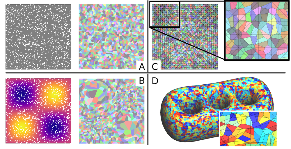
Figure 12: A: transport between a uniform density and a random pointset; B: transport between a varying density and the same pointset; C: intersections between meshes used to compute the coefficients; D: transport between a measure supported by a surface and a 3D pointset.

Figure 13: Interpolation of 3D volumes using optimal transport.

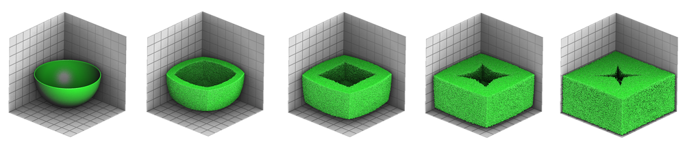
Figure 14: Computing the transport between objects of different dimension, from a sphere to a cube. The sphere is sampled with 10 million points. The cross-section reveals the formation of a singularity that has some similarities with the medial axis of the cube.

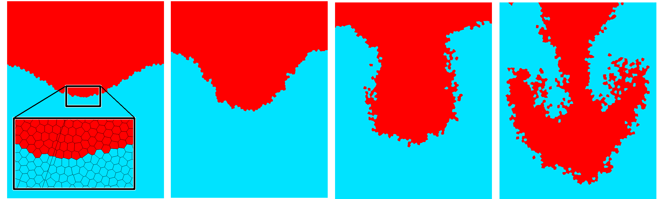
Figure 15: An application of optimal transport to fluid simulation: numerical simulation of the Taylor-Rayleigh instability using the Gallouet-Mérigot scheme.

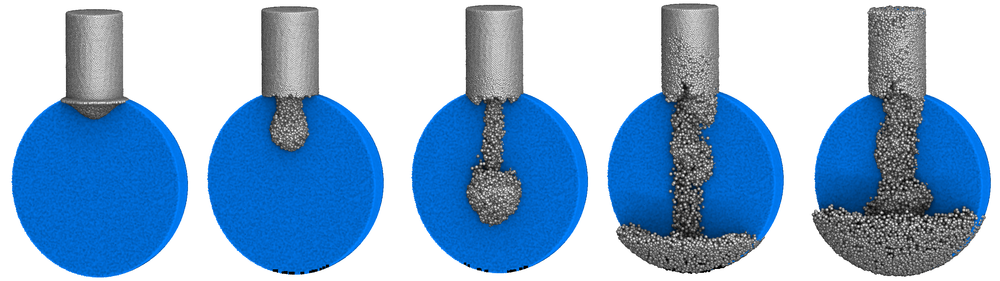
Figure 16: Numerical simulation of an incompressible bi-phasic flow in a bottle.

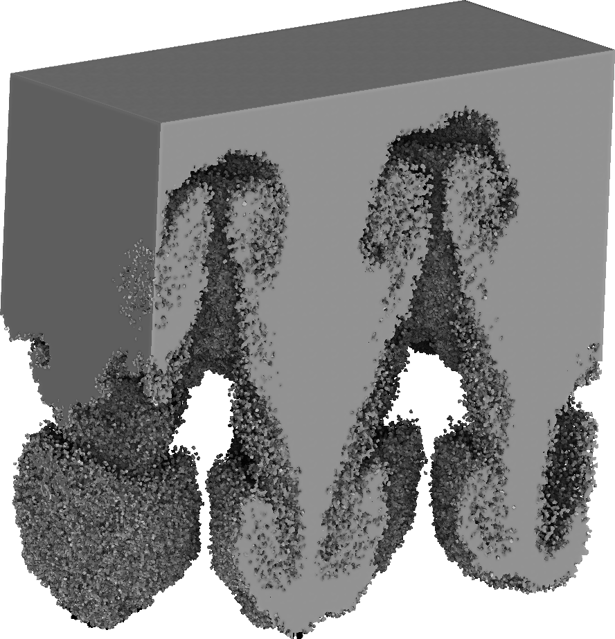
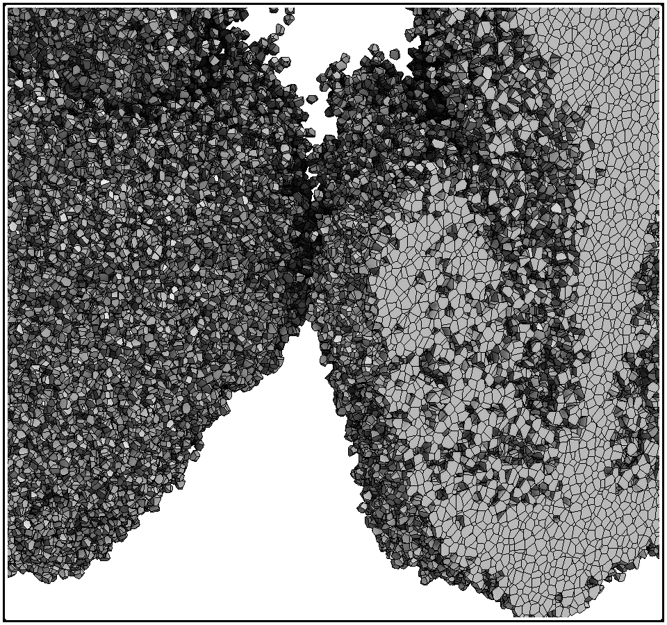
Figure 17: Top: Numerical simulation of the Taylor-Rayleigh instability using a 3D version of the Gallouet-Mérigot scheme, with a cross-section that reveals the internal structure of the vortices. Bottom: a closeup that shows the interface between the two fluids, represented by the Laguerre facets that bound two Laguerre cells of different fluid elements.

Figure 12 shows some examples of transport in 2D, between a uniform density and a pointset (A). Each Laguerre cell has the same area. Then we consider the same pointset, but this time with a density $u(x,y)=10(1+\sin(2\pi x)\sin(2\pi y))$ (image B). We obtain a completely different Laguerre diagram. Each cell of this diagram has the same value for the integrated density $u$. (C): the coefficients of the gradient and the Hessian of $F$ computed in the previous section involve integrals of the density $u$ over the Laguerre cells and over their boundaries. The density $u$ is supported by a triangulated mesh, and linearly interpolated on the triangles. The integrals of $u$ over the Laguerre cells and their boundaries are evaluated in closed form, by computing the intersections between the Laguerre cells and the triangles of the mesh that supports $u$. (D): the same algorithm can compute the optimal transport between a measure supported by a 3D surface and a pointset in 3D.

Figure 13 shows two examples of volume deformation by optimal transport. The same algorithm is used, but this time with 3D Laguerre diagrams, and by computing intersections between the Laguerre cells and a tetrahedral mesh that supports the source density $u$. The intermediary steps of the animation are generated by linear interpolation of the positions (Mc. Cann’s interpolation). Figure 14 demonstrates a more challenging configuration, computing transport between a sphere (surface) and a cube (volume). The sphere is approximated with 10 million Dirac masses. As can be seen, transport has a singularity that resembles the medial axis of the cube (rightmost figure).

Figure 15 demonstrates an application in computational fluid dynamics. A heavy incompressible fluid (in red) is placed on top of a lighter incompressible fluid (in blue). Both fluids tend to exchange their positions, due to gravity, but incompressibility is an obstacle to their movement. As a result, vortices are created, and they become faster and faster (Taylor-Rayleigh instability). The numerical simulation method that we used here [GM17] directly computes the trajectories of particles (Lagrangian coordinates) while taking into account the incompressibility constraint, which is in general unnatural in Lagrangian coordinates. By providing a means of controlling the volumes of the Laguerre cells, optimal transport appears here as an easy way of enforcing incompressibility. Using some efficient geometric algorithms for the Laguerre diagram and its intersections [Lév15], the Gallouet-Mérigot numerical scheme for incompressible Euler scheme can be also applied in 3D to simulate the behavior of non-mixing incompressible fluids (Figure 16). The 3D version of the Taylor-Rayleigh instability is shown in Figure 17, with 10 million Laguerre cells. More complicated vortices are generated (shown here in cross-section).

The applications in computer animation and computational physics seem to be promising, because the semi-discrete algorithm behaves very well in practice. It is now reasonable to design simulation algorithms that solve a transport problem in each timestep (as our early computational fluid dynamics of the previous paragraph do). With our optimized implementation that uses a multicore processor for the geometric part of the algorithm and a GPU for solving the linear systems, the semi-discrete algorithm takes no more than a few tens of seconds to solve a problem with 10 millions unknown. This opens the door to numerical solution mechanisms for difficult problems. For instance, in astrophysics, the Early Universe Reconstruction problem [BFH⁺03] consists in going “backward in time” from observation data on the repartition of galaxy clusters, to “play the Big-Bang movie” backward. Our numerical experiments tend to confirm Brenier’s point of view that he expressed in the 2000’s, that semi-discrete optimal transport can be an efficient way of solving this problem.

To ensure that our results are reproducible, the source-code associated with the numerical solution mechanism used in all these experiments is available in the EXPLORAGRAM component of the GEOGRAM programming library.

References

- [AG13] Luigi Ambrosio and Nicolas Gigli. A user’s guide to optimal transport. Modelling and Optimisation of Flows on Networks, Lecture Notes in Mathematics, pages 1–155, 2013.
- [AHA92] Franz Aurenhammer, Friedrich Hoffmann, and Boris Aronov. Minkowski-type theorems and least-squares partitioning. In Symposium on Computational Geometry, pages 350–357, 1992.
- [Ale05] A. D. Alexandrov. Intrinsic geometry of convex surfaces (translation of the 1948 Russian original). CRC Press, 2005.
- [Aur87] Franz Aurenhammer. Power diagrams: Properties, algorithms and applications. SIAM J. Comput., 16(1):78–96, 1987.
- [BB00] Jean-David Benamou and Yann Brenier. A computational fluid mechanics solution to the monge-kantorovich mass transfer problem. Numerische Mathematik, 84(3):375–393, 2000.
- [BCMO14] Jean-David Benamou, Guillaume Carlier, Quentin Mérigot, and Edouard Oudet. Discretization of functionals involving the monge-ampère operator. arXiv, August 2014. [math.NA] http://arxiv.org/abs/1408.4336.
- [BDM09] Rainer Burkard, Mauro Dell’Amico, and Silvano Martello. Assignment Problems. SIAM, 2009.
- [BFH+03] Y. Brenier, U. Frisch, M. Henon, G. Loeper, S. Matarrese, R. Mohayaee, and A. Sobolevskii. Reconstruction of the early universe as a convex optimization problem. arXiv, September 2003. arXiv:astro-ph/0304214v3.
- [Bow81] Adrian Bowyer. Computing dirichlet tessellations. Comput. J., 24(2):162–166, 1981.
- [Bre91] Yann Brenier. Polar factorization and monotone rearrangement of vector-valued functions. Communications on Pure and Applied Mathematics, 44:375–417, 1991.
- [BvdPPH11] Nicolas Bonneel, Michiel van de Panne, Sylvain Paris, and Wolfgang Heidrich. Displacement interpolation using lagrangian mass transport. ACM Trans. Graph., 30(6):158, 2011.
- [Caf03] Luis Caffarelli. The monge-ampère equation and optimal transportation, an elementary review. Optimal transportation and applications (Martina Franca, 2001), Lecture Notes in Mathematics, pages 1–10, 2003.
- [Cut13] Marco Cuturi. Sinkhorn distances: Lightspeed computation of optimal transport. In Advances in Neural Information Processing Systems 26: 27th Annual Conference on Neural Information Processing Systems 2013. Proceedings of a meeting held December 5-8, 2013, Lake Tahoe, Nevada, United States., pages 2292–2300, 2013.
- [dGWH+15] Fernando de Goes, Corentin Wallez, Jin Huang, Dmitry Pavlov, and Mathieu Desbrun. Power particles: an incompressible fluid solver based on power diagrams. ACM Trans. Graph., 34(4):50:1–50:11, 2015.
- [GM96] Wilfrid Gangbo and Robert J. McCann. The geometry of optimal transportation. Acta Math., 177(2):113–161, 1996.
- [GM17] Thomas O. Gallouët and Quentin Mérigot. A lagrangian scheme à la Brenier for the incompressible euler equations. Foundations of Computational Mathematics, May 2017.
- [HS52] Magnus R. Hestenes and Eduard Stiefel. Methods of Conjugate Gradients for Solving Linear Systems. Journal of Research of the National Bureau of Standards, 49(6):409–436, December 1952.
- [KMT16] Jun Kitagawa, Quentin Mérigot, and Boris Thibert. A newton algorithm for semi-discrete optimal transport. CoRR, abs/1603.05579, 2016.
- [Leo13] Christian Leonard. A survey of the schrödinger problem and some of its connections with optimal transport. arXiv, August 2013. [math.PR] http://arxiv.org/abs/1308.0215.
- [Lév15] Bruno Lévy. A numerical algorithm for semi-discrete optimal transport in 3d. ESAIM M2AN (Mathematical Modeling and Analysis), 2015.
- [McC95] Robert J. McCann. Existence and uniqueness of monotone measure-preserving maps. Duke Mathematical Journal, 80(2):309–323, 1995.
- [Mém11] Facundo Mémoli. Gromov-wasserstein distances and the metric approach to object matching. Foundations of Computational Mathematics, 11(4):417–487, 2011.
- [Mér11] Quentin Mérigot. A multiscale approach to optimal transport. Comput. Graph. Forum, 30(5):1583–1592, 2011.
- [MMT17] Quentin Mérigot, Jocelyn Meyron, and Boris Thibert. Light in power: A general and parameter-free algorithm for caustic design. CoRR, abs/1708.04820, 2017.
- [Mon84] Gaspard Monge. Mémoire sur la théorie des déblais et des remblais. Histoire de l’Académie Royale des Sciences (1781), pages 666–704, 1784.
- [NW06] J. Nocedal and S. J. Wright. Numerical Optimization. Springer, New York, 2nd edition, 2006.
- [PPO14] Nicolas Papadakis, Gabriel Peyré, and Edouard Oudet. Optimal Transport with Proximal Splitting. SIAM Journal on Imaging Sciences, 7(1):212–238, January 2014.
- [San14] Filippo Santambrogio. Introduction to Optimal Transport Theory. In Optimal Transport, Theory and Applications, August 2014. [math.PR] http://arxiv.org/abs/1009.3856.
- [San15] Filippo Santambrogio. Optimal transport for applied mathematicians, volume 87 of Progress in Nonlinear Differential Equations and their Applications. Birkhäuser/Springer, Cham, 2015. Calculus of variations, PDEs, and modeling.
- [STTP14] Yuliy Schwartzburg, Romain Testuz, Andrea Tagliasacchi, and Mark Pauly. High-contrast computational caustic design. ACM Trans. Graph., 33(4):74:1–74:11, 2014.
- [Tao11] Terence Tao. An Introduction to Measure Theory. American Mathematical Society, 2011.
- [Vil09] Cédric Villani. Optimal transport : old and new. Grundlehren der mathematischen Wissenschaften. Springer, Berlin, 2009.
- [Wat81] David Watson. Computing the n-dimensional delaunay tessellation with application to voronoi polytopes. Comput. J., 24(2):167–172, 1981.