The KPP boundary layer scheme: revisiting its formulation and benchmarking one-dimensional ocean simulations relative to LES

Abstract

We evaluate the Community ocean Vertical Mixing (CVMix) project version of the K-profile parameterization (KPP). For this purpose, one-dimensional KPP simulations are compared across a suite of oceanographically relevant regimes against large eddy simulations (LES). The LES is forced with horizontally uniform boundary fluxes and has horizontally uniform initial conditions, allowing its horizontal average to be compared to one-dimensional KPP tests. We find the standard configuration of KPP (Danabasoglu et al., 2006) consistent with LES across many forcing regimes, supporting the physical basis of KPP. Our evaluation motivates recommendations for ”best practices” for using KPP within ocean circulation models, and identifies areas where further research is warranted. Further, our test suite can be used as a baseline for evaluation of a broad suite of boundary layer models.

The original treatment of KPP recommends the matching of interior diffusivities and their gradients to the KPP predicted values computed in the ocean surface boundary layer (OSBL). However, we find that difficulties in representing derivatives of rapidly changing diffusivities near the base of the OSBL can lead to loss of simulation fidelity. We propose two alternative approaches: (1) match to the internal predicted diffusivity along, (2) set the KPP diffusivity to zero at the OSBL base. Although computationally simpler, the second alternative is sensitive to implementation details and we offer methods to prevent the emergence of numerical high frequency noise.

We find the KPP entrainment buoyancy flux to be sensitive to vertical grid resolution and details of how to diagnose the KPP boundary layer depth. We modify the KPP turbulent shear velocity parameterization to reduce resolution dependence. Additionally, our results show that the KPP parameterized non-local tracer flux is incomplete due to the assumption that it solely redistributes the surface tracer flux. However, examination of the LES vertical turbulent scalar flux budgets show that non-local fluxes can exist in the absence of surface tracer fluxes. This result motivates further studies of the non-local flux parameterization.

Journal of Advances in Modeling Earth Systems (JAMES)

Fluid Dynamics and Solid Mechanics, Los Alamos National Laboratory, Los Alamos, NM, LA-UR-16-26992 NOAA / Geophysical Fluid Dynamics Laboratory, Princeton, NJ and Princeton University Program in Atmospheric and Oceanic Sciences, Princeton, NJ Climate and Global Dynamics Laboratory, National Center for Atmospheric Research, Boulder, CO Leibniz-Institute of Baltic Sea Research, Warnemünde, Seestraße 15, 18119, Rostock, Germany

Luke Van Roekellvanroekel@lanl.gov

The Community ocean Vertical Mixing (CVMix) project version of the K-profile parameterization (KPP) is compared across a suite of oceanographically relevant regimes against large eddy simulations (LES).

The standard configuration of KPP is consistent with LES results across many simulations, but some adaptations of KPP for improved applicability relative to LES comparisons are proposed.

An alternate, computationally simpler, configuration of KPP is proposed to alleviate the need to represent rapidly changing diffusivities near the base of the ocean surface boundary layer.

Draft from

1 Introduction

The ocean surface boundary layer (OSBL) mediates momentum, heat, and scalar tracer fluxes between the interior ocean with the atmosphere and cryosphere. Consequently, an accurate parameterization of turbulence and the induced vertical mixing in the OSBL is essential for robust model simulations of climate physics and of the abundance and distribution of important biological and chemical quantities. We here consider the formulation and behavior of the K-profile parameterization (KPP) (Large et al., 1994, LMD94), which has been used by a variety of ocean and climate applications. Here we consider one-dimensional vertical fluxes only. KPP fidelity in the presence of horizontal features (e.g., baroclinic fronts; Bachman et al., 2017) is not considered.

1.1 The suite of boundary layer parameterizations

Generally, boundary layer parameterizations like KPP assume the turbulent mixing is dominated by vertical fluxes. Presently, varying degrees of complexity are used to parameterize these fluxes. Bulk boundary layer models are perhaps the simplest (e.g., Kraus and Turner, 1967; Niiler and Kraus, 1977; Price et al., 1986; Gaspar, 1988), where ocean properties (tracers and momentum) are assumed to be vertically uniform in the OSBL. The assumption of no vertical structure within the boundary layer is both the key simplification and the main deficiency of bulk models. Namely, ocean tracers and momentum are not generally uniform vertically, even in the presence of strong mixing. Hence, vertical integration over the depth of the OSBL precludes the simulation of OSBL processes such as the Ekman spiral and boundary layer restratification (but see Hallberg, 2003, for a proposed method to remedy these deficiencies).

Turbulence Kinetic Energy (TKE) closure (TC) is another widely used framework for parameterizing upper ocean boundary layer mixing (e.g., Kantha and Clayson, 1994; Canuto et al., 2001; Umlauf and Burchard, 2005; Canuto et al., 2007; Harcourt, 2015). In most variants of TC, the profiles of eddy diffusivity and viscosity are dependent on the local TKE, which is prognostic (e.g., Mellor and Yamada, 1982; Kantha and Clayson, 1994). Most of these models are local as the turbulent fluxes of tracers and momentum exist only in the presence of non-zero vertical gradients of the mean quantities. Yet in highly convective conditions strong fluxes exist even when $\partial\theta/\partial z\approx 0$. Thus many TC models are deficient in highly convective conditions, as they predict zero flux through much of the boundary layer. However, a few TC models (e.g., Stull, 1993; Lappen and Randall, 2001; Soares et al., 2004) do include non-local mixing effects.

The K-profile parameterization (KPP) (Large et al., 1994, hereafter LMD94) aims to represent a middle ground between bulk boundary layer models and prognostic TC models. KPP allows for vertical property variations in the OSBL via a specified vertical shape function (O’Brien, 1970). KPP includes a parameterized non-local transport allowing for the existence of vertical turbulent scalar fluxes in the absence of vertical gradients of scalar quantities.

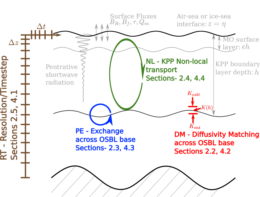
Figure 1: Schematic of the upper ocean regions associated with the KPP boundary layer parameterization. The upper ocean is exposed to fluxes of momentum, $\tau$, mass, $Q_{m}$, and buoyancy, $B_{f}$, at the air-sea interface. Penetrating shortwave radiation, $(\overline{w^{\prime}\theta^{\prime}})_{R}$, along with its associated buoyancy flux, $B_{R}>0$, also influence the upper ocean. The Monin-Obukhov (MO) surface layer transfers these fluxes to the remainder of the boundary layer. Here we assume the surface layer extends from the free surface ($z=\eta$) to $z=\eta-\epsilon h$, where $h>0$ is the depth of the boundary layer base (typically $\epsilon\approx 0.1$). The colored portions of the schematic represent the four components of KPP we focus on in this paper (Section 2). The red section represents the diffusivity matching in KPP, where $K_{osbl}$, $K_{int}$, and $K(h)$ are the diffusivities at the last layer in the OSBL, the first model layer below the OSBL, and at the OSBL respectively. The green signifies the non-local parameterization, the blue represents entrainment and detrainment across the OSBL base, and the brown represents the influence of choices in the calling model on KPP fidelity. The sections for each color denotes the portions of the paper where that process is examined.

1.2 The CVMix Project

KPP has been implemented in numerous ocean circulation models. In our experience, each implementation makes slightly distinct physical and numerical choices. Sometimes, these implementation choices have unintended consequences that can negatively impact the KPP boundary layer simulation. This situation provided the mandate for our development of KPP within the CVMix project (Griffies et al., 2015), and the examination of that implementation in this paper.

The CVMix library is developed as a suite of standardized vertical mixing parameterizations to be implemented in a three-dimensional ocean circulation model. As a part of the CVMix development, our purpose here is to evaluate the influence of physical assumptions and numerical choices within the CVMix version of KPP as well as in the ocean circulation model. The present paper serves to document many of our findings.

1.3 An LES evaluation framework for OSBL parameterizations

Large Eddy Simulations (LES) provide our evaluation framework for the KPP scheme. As configured here, the LES resolves the dominant eddies and with sub-grid turbulence small relative to that realized at resolved scales. The LES is forced with horizontally uniform surface fluxes and the output is horizontally and temporally averaged. We compare the LES results to one-dimensional KPP simulations using identical forcing and initialization. Numerous studies have compared atmospheric boundary layer parameterizations to LES (e.g., Holtslag and Moeng, 1991; Moeng and Sullivan, 1994; Brown, 1996; Ayotte et al., 1996; Noh et al., 2003), with far fewer LES evaluations of ocean parameterizations. Those ocean LES comparisons have made similar (and limited) initial conditions and forcing scenarios (e.g., McWilliams and Sullivan, 2000; Smyth et al., 2002; Reichl et al., 2016; Bachman et al., 2017). Our somewhat larger test suite facilitates an examination of the KPP under a broader range of forcing scenarios.

Following atmospheric comparisons (e.g., Ayotte et al., 1996), we use a suite of forcing and initial conditions. However, our LES configuration precludes the examination of interactions with horizontal processes in the boundary layer, such as from submesoscale frontal instabilities (e.g., Boccaletti et al., 2007; Fox-Kemper et al., 2008; Bachman et al., 2017). Instead, we focus on examining the influence of physical assumptions within KPP as well as numerical implementation choices.

We test the CVMix implementation of KPP against LES configured with similar depth and surface forcing. Furthermore, simulation differences can arise due to details of how KPP is embedded within the calling model. We thus compare KPP as realized in three ocean circulation models: Model for Prediction Across Scales - Ocean (MPAS-O; (Ringler et al., 2013)); Modular Ocean Model Version 6 (MOM6; (Adcroft and Hallberg, 2006)); and Parallel Ocean Program Version 2 (POP2; (Smith et al., 2010)). We found these details explain some differences in behavior relative to LMD94, and thus they are important for evaluating the integrity of KPP and for choosing its parameters.

1.4 Organization of this paper

We start the main portion of this paper in Section 2, where we summarize elements of KPP and present salient implementation considerations and issues that arose in our development and evaluation. We then present a few sections that document our experiences benchmarking KPP against LES. We discuss the test cases and LES model in Section 3, and then describe results and analysis in Sections 4-6. The presentation of results focuses on issues discussed in Section 2 and offers possible solutions. We close the main portion of the paper with conclusions and best practice recommendations in Section 7, and then with suggested future KPP developments in Section 8. Various appendices offer further details about aspects of the KPP scheme and the test cases.

2 KPP considerations

The implementation of KPP within CVMix closely follows that detailed in LMD94, including the modifications of Danabasoglu et al. (2006). We present here some salient points that elucidate implementation considerations and introduce issues that arose during our CVMix development. Further formulation details of the KPP scheme are given in Appendix A, and a Table of symbols along with preferred units is given in Appendix B.

2.1 Basic definitions

The vertical position in the ocean, $z$, ranges from

$$-H(x,y)\leq z\leq\eta(x,y,t)$$ (1)

where $z=-H$ is the position of the static ocean bottom, $z=\eta$ is the position for the dynamic ocean free surface, $z=0$ is the resting ocean surface (reference geopotential), and

$$\mbox{depth}=-z+\eta\geq 0$$ (2)

is the positive distance from the ocean surface to a point in the ocean. When referring to positions within the surface boundary layer, it is convenient to use a non-dimensional boundary layer coordinate

$$\sigma\equiv\frac{-z+\eta}{h}\qquad 0\leq\sigma\leq 1,$$ (3)

where $\sigma=0$ at the ocean free surface and $\sigma=1$ at the boundary layer base where

$$-z+\eta=h\qquad\mbox{OSBL thickness}.$$ (4)

2.2 General structure of the KPP parameterization

For any prognostic scalar or vector field component $\psi$ (e.g., velocity components, tracer concentrations), the KPP scheme parameterizes the turbulent vertical flux within the surface boundary layer according to

$$\overline{w^{\prime}\psi^{\prime}}=-K_{\psi}\frac{\partial\psi}{\partial z}+K_{\psi}\gamma_{\psi}.$$ (5)

In this equation, the first term represents the local contribution to the turbulent vertical flux of $\psi$, and the second term is the parameterized non-local flux. The eddy diffusivity $K_{\psi}$ is written as the product of three terms

$$K_{\psi}=h\,w_{\psi}\left(\sigma\right)G\left(\sigma\right),$$ (6)

where $h$ is the KPP diagnosed OSBL depth (equation (4), and $G(\sigma)$ is the vertical shape function.

Equations (5)-(6) suggest a few important considerations in the implementation of KPP. For example, the boundary layer depth $h>0$ scales the diffusivity, so that the maximum $K_{\psi}$ is larger for deeper boundary layers, suggesting that KPP is critically dependent on the boundary layer depth. Further, the vertical structure of the KPP diffusivity and hence the non-local flux is set by the non-dimensional shape function, $G(\sigma)$, which is scaled by the boundary layer depth.

In this work we focus on four main physical and numerical processes colored in Figure 1:

• matching the diffusivity and its gradient (DM) at the OSBL base (red);

• property exchange (PE; i.e., entrainment and detrainment) across the OSBL base (blue);

• non-local (NL) transport (green);

• model resolution and timestep (RT; brown).

Given that all of the processes in Figure 1 are influenced by the KPP-diagnosed OSBL depth, the KPP OSBL depth algorithm is pivotal and discussed in some detail in Section 2.3. Our four focus areas are introduced in the following subsections.

2.3 Bulk Richardson number and the boundary layer depth

In KPP, the bulk Richardson number is computed by

$$\mbox{Ri}_{\mbox{\tiny b}}=\frac{(b_{\tiny\mbox{sl}}-b(z))\,(-z+\eta)}{|\mathbf{u}_{\tiny\mbox{sl}}-\mathbf{u}(z)|^{2}+V_{t}^{2}(z)}.$$ (7)

In this expression, $b$ is the buoyancy (dimensions of length per squared time) based on the surface referenced potential density, and $b_{\tiny\mbox{sl}}$ is the buoyancy averaged over the depth of the surface layer between the depth range $0\leq\sigma\leq\epsilon$ (see Figure 1). Small differences of $b_{\tiny\mbox{sl}}-b(z)$ signal weak vertical stratification, characteristic of a region within the surface boundary layer. In contrast, large differences arise when $z$ reaches into the more stratified region beneath the boundary layer. The denominator in $\mbox{Ri}_{\mbox{\tiny b}}$ consists of the squared vertical shear resolved by the model’s prognostic horizontal velocity field: $|\mathbf{u}_{\tiny\mbox{sl}}-\mathbf{u}(z)|^{2}$, where $\mathbf{u}_{\tiny\mbox{sl}}$ is the surface layer averaged horizontal velocity. In addition, the term $V_{t}^{2}$ aims to parameterize unresolved vertical shears near the OSBL base (see Section 2.5.1). When either the resolved or parameterized shear is large, the bulk Richardson number is small and the OSBL deepens. Finally, note that even if the buoyancy difference and vertical shear are vertically constant, the bulk Richardson number increases linearly with depth, $d=-z+\eta$, given the presence of depth in the numerator of equation (7).

The depth at the base of the ocean surface boundary layer, $-z+\eta=h$, is computed as the depth where the bulk Richardson number equals a critical value

$$\mbox{Ri}_{\mbox{\tiny b}}=\mbox{Ri}_{\mbox{\tiny crit}}=\frac{(b_{\tiny\mbox{\tiny\mbox{sl}}}-b(h))\,h}{|\mathbf{u}_{\tiny\mbox{\tiny\mbox{sl}}}-\mathbf{u}(h)|^{2}+V_{t}^{2}(h)}.$$ (8)

In LMD94, the critical bulk Richardson number was set to $\mbox{Ri}_{\mbox{\tiny crit}}=0.3$. However, values between 0.25 and 1.0 have been used in similar formulations (e.g., Troen and Mahrt, 1986; Vogelzang and Holtslag, 1996; McGrath-Spangler et al., 2015). In general, the correct diagnosis of the boundary layer depth is a key part of the KPP scheme, as this depth controls the upper ocean turbulent layer and the strength of mixing within that layer. The diagnosed boundary layer depth also controls the strength of entrainment into the OSBL. We thus expect the chosen definitions of surface layer fraction ($\epsilon$; Figure 1), parameterized turbulent vertical shear, $V_{t}^{2}$, and the critical bulk Richardson number, $\mbox{Ri}_{\mbox{\tiny crit}}$, to strongly influence KPP results and their comparison to LES.

Values of $\mbox{Ri}_{\mbox{\tiny crit}}$ vary from $\mbox{Ri}_{\mbox{\tiny crit}}=0.25$ for shear instability when using a linear stability analysis (Miles, 1961) to O(1) for a non-linear stability analysis (Abarbanel et al., 1984). However, Troen and Mahrt (1986) argue that shear may not be adequately resolved in a model simulation, prompting use of a larger value of $\mbox{Ri}_{\mbox{\tiny crit}}$ that is a function of vertical grid spacing.

Further, it is unlikely that the bulk Richardson number computed at a model interface is exactly equal to the chosen critical threshold. Consequently, the KPP boundary layer depth, $h$, will also be sensitive to the interpolation method used to determine where $\mbox{Ri}_{\mbox{\tiny b}}=\mbox{Ri}_{\mbox{\tiny crit}}$ according to equation (8) (Danabasoglu et al., 2006; Seidel et al., 2010). For direct comparison between KPP and LES we use the KPP bulk Richardson number method based on equation (8) to determine the OSBL depth with LES data.

2.4 Shape function and diffusivity matching

The vertical shape function ($G(\sigma)$) controls the vertical structure of diffusivity and the non-local flux in KPP (equation (6)). The shape function is assumed to follow a cubic polynomial as proposed by O’Brien (1970). The method to determine all of the coefficients of the polynomial is given in Appendix A.1 and LMD94. Here we identify potential issues with the matching of diffusivities from KPP to those determined by interior mixing parameterizations.

2.4.1 Problems matching diffusivity derivatives at the OSBL base

The KPP diffusivity matching proposed by LMD94 means that parameterized turbulence generated in the ocean interior (e.g., internal waves, shear instabilities) indirectly influences that in the surface boundary layer. Given that the interior diffusivity can have nontrivial vertical structure, its vertical gradient can be large and potentially negative. Hence, there is no guarantee that the KPP diffusivity will vary smoothly across the OSBL base. Further, the vertical derivative of the diffusivity can be sharp (i.e., discontinuous) near the OSBL base, which leads to a generally poor representation on a discrete vertical grid. Therefore, given these potential difficulties we test the sensitivity of KPP to three variants of internal matching: matching the internal diffusivity and its gradient, matching the internal diffusivity alone, and abandoning internal matching in section 5.2.

2.4.2 Problems with the non-local parameterization at the OSBL base

If the KPP computed boundary layer diffusivities (and the derivatives) are forced to match the corresponding interior values, the vertical shape function, $G(\sigma)$, is not guaranteed to be zero at the base of the boundary layer, $G(\sigma=1)\neq 0$. A non-zero $G(1)$ is not desirable since it leads to a non-local flux at the boundary layer base. The non-local flux should vanish at the base of the boundary layer since that is the depth at which boundary layer turbulence vanishes.

Neglecting diffusivity matching at the OSBL base would resolve this inconsistency for the non-local term. As a physical justification for dropping the diffusivity matching, one may assume that KPP is only parameterizing effects from the larger and stronger turbulent boundary layer eddies. Other interior mixing parameterizations (e.g, the LMD94 shear instability mixing scheme) could be assumed to be scale separated from KPP as KPP seeks to parameterize penetration of the most unstable eddies. Under this assumption, the net diffusivity in the OSBL is computed as the sum of that predicted by KPP plus other parameterizations. In Section 5.2, we examine a configuration of KPP where diffusivity matching is neglected.

2.5 Property exchanges across the OSBL base

Property exchanges at the OSBL base are determined in two ways: a parameterization of unresolved turbulence ($V_{t}^{2}$) and the enhanced diffusivity parameterization. The former exerts a strong influence at high vertical resolution, while the latter dominates at coarser vertical resolution. We discuss both in this section.

2.5.1 The parameterization of $V_{t}^{2}$ in $\mbox{Ri}_{\mbox{\tiny b}}$

The KPP scheme includes a term related to an energy associated with unresolved turbulence ($V_{t}^{2}$) in the bulk Richardson number denominator in equation (7). The purpose of this term is to sufficiently deepen the OSBL to ensure that the empirical rule of convection (see LMD94) is satisfied. This rule says that the minimum turbulent buoyancy flux within the boundary layer is given by

$$\overline{w^{\prime}b^{\prime}}_{\mbox{\tiny$h_{e}$}}\approx-0.2\,\overline{w^{\prime}b^{\prime}}_{\mbox{\tiny sfc}},$$ (9)

where $h_{e}$ is the entrainment depth (see Figure 2). The entrainment depth is where water from below the boundary layer is exchanged with boundary layer water. The entrainment depth is also the depth of the minimum buoyancy flux.

The parameterization of $V_{t}^{2}$ is derived by considering a buoyancy profile that is well-mixed to a given depth ($h_{m}$) with linear stratification below (Figure 2). The buoyancy flux at $h_{e}$ is written (using equations (5) and (6)) as

$$\overline{w^{\prime}b^{\prime}}_{\mbox{\tiny$h_{e}$}}=-h\,w_{s}(\sigma)\,G(\sigma)\,\left(\frac{\partial b}{\partial z}-\gamma_{b}\right)\qquad\mbox{with}\;\;\sigma=\frac{h_{e}}{h}.$$ (10)

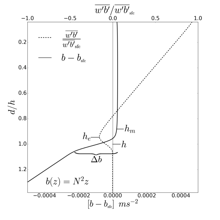
Figure 2: Schematic illustrating the various depths arising in the boundary layer as forced by a destabilizing surface buoyancy flux $\overline{w^{\prime}b^{\prime}}_{\mbox{\tiny sfc}}<0$ (defined in equation (24)). This forcing supports active non-local convective boundary layer turbulence. Data for this figure is taken from the LES results of the FC experiment (Figure 3a). The vertical axis is the non-dimensional boundary layer depth, $\sigma=(-z+\eta)/h$, extending from beneath the boundary layer ($\sigma>1$) to the base of the surface layer ($\sigma=\epsilon\,h$) (see Figure 1). The dashed line is the local turbulent buoyancy flux, $(\overline{w^{\prime}b^{\prime}})$, normalized by the surface buoyancy flux $(\overline{w^{\prime}b^{\prime}}_{\mbox{\tiny sfc}})$. The scale for this ratio is along the top axis. Depths where $\overline{w^{\prime}b^{\prime}}/\overline{w^{\prime}b^{\prime}}_{\mbox{\tiny sfc}}<0$ are where the local turbulence stabilizes the boundary layer, which occurs near the boundary layer base. The solid line is the difference in local buoyancy and the surface layer buoyancy, $b-b_{\mbox{\tiny sfc}}$, with corresponding scale along the bottom axis (in units of $10^{-4}$ $\mbox{m}~{}\mbox{s}^{-2}$). The mixed layer is where buoyancy is weakly stratified, $\partial b/\partial z\approx 0$. The mixed layer base is determined subjectively by $\partial b/\partial z>(\partial b/\partial z)_{\mbox{\tiny min}}>0$, with $(\partial b/\partial z)_{\mbox{\tiny min}}$ a chosen minimum stratification criteria. For much of the boundary layer, $b-b_{\mbox{\tiny sfc}}>0$, since the surface layer buoyancy is driven low by the destabilizing surface flux. The entrainment depth, $h_{e}$, is where $\overline{w^{\prime}b^{\prime}}/\overline{w^{\prime}b^{\prime}}_{\mbox{\tiny sfc}}<0$ reaches a minimum, with $h_{e}$ straightforward to diagnose in a LES. (See E for an idealized buoyancy profile similar to that shown here allowing for an analytic expression for $h$). In the entrainment layer, buoyancy changes rapidly ($\Delta b$), reflecting enhanced vertical stratification below the mixed layer. Below the entrainment layer, the buoyancy profile is roughly constant ($b\approx N^{2}\,z$ with $N^{2}>0$ constant and $z<0$). The KPP boundary layer depth, $h$, is determined by the bulk Richardson number criteria in equation (8).

Near the boundary layer depth, $h$, the non-local term $\gamma_{b}$ (see equation (18)) is small and can be ignored. Furthermore, in convective conditions,

$$w_{b}(h_{e}/h)\rightarrow\kappa\left(c_{s}\,\kappa\,\epsilon\right)^{1/3}w_{*}\,,$$ (11)

where $\kappa$ is the von Kármán constant, $c_{s}$ is an empirical constant, and $w_{*}$ is the convective turbulent velocity scale defined as

$$w_{*}\equiv(-h\,\overline{w^{\prime}b^{\prime}}_{\mbox{\tiny sfc}})^{1/3}.$$ (12)

Also, noting that $N_{osbl}^{2}=(\partial b/\partial z)_{osbl}$ and $h_{e}/h\approx 1$, equation (10) becomes

$$\overline{w^{\prime}b^{\prime}}_{h_{e}} = -\kappa\left(c_{s}\kappa\epsilon\right)^{1/3}w_{*}\,\left(1-\frac{h_{e}}{h}\right)^{2}\,h\,N_{osbl}^{2}$$ (13)

$$= -\kappa\left(c_{s}\kappa\epsilon\right)^{1/3}w_{*}\left(h-h_{e}\right)^{2}N_{osbl}^{2}/h.$$

At the OSBL base, $\mbox{Ri}_{\mbox{\tiny b}}=\mbox{Ri}_{\mbox{\tiny crit}}$ (see equation (8)). We can use this result to write an equation for $V_{t}^{2}$. By assuming the resolved vertical shear is zero we have

$$\mbox{Ri}_{\mbox{\tiny crit}}=\frac{h\,(b_{\tiny\mbox{sl}}-b(h))}{V_{t}^{2}}.$$ (14)

Given the assumed linear buoyancy profile, the numerator of equation (14) is $h\,N_{osbl}^{2}(h-h_{e})$, which implies

$$h-h_{e}=\frac{V_{t}^{2}\,\mbox{Ri}_{\mbox{\tiny crit}}}{h\,N_{osbl}^{2}}.$$ (15)

Using equations (14) and (15) brings equation (13) into the form

$$\overline{w^{\prime}\,b^{\prime}}_{\mbox{\tiny$h_{e}$}}=-\kappa\left(c_{s}\kappa\epsilon\right)^{1/3}w_{*}\,V_{t}^{4}\,\mbox{Ri}_{\mbox{\tiny crit}}^{2}\,N_{osbl}^{2}/(N_{osbl}^{4}\,h^{3}).$$ (16)

If the empirical rule of convection (equation (9)) is enforced in (16), the result can be solved for $V_{t}^{2}$ so that

$$V_{t}^{2}=\frac{\sqrt{0.2}\,C_{v}}{\mbox{Ri}_{\mbox{\tiny crit}}\,\kappa^{2/3}}\left(c_{s}\,\epsilon\right)^{-1/6}\,h\,N_{osbl}\,w_{*}$$ (17)

where LMD94 included the constant $C_{v}$ to account for smoothing of the buoyancy profile near $h_{e}$ due to mixing.

Note here that $N_{osbl}$ is the stratification near $h_{e}<h$. This approach contrasts to the use of stratification below the OSBL as suggested by Danabasoglu et al. (2006) (their Appendix A). Both options are tested relative to LES in Sections 5.1.2.

2.5.2 Enhanced diffusivity

For coarse vertical resolution, LMD94 propose the addition of an enhanced diffusivity to partially mitigate resolution-dependent biases. Here we suggest that the enhanced diffusivity parameterization also serves to parameterize unresolved sources of entrainment.

In their Appendix D, LMD94 note that as vertical resolution coarsens near the OSBL base, ”staircase” structures can emerge in the time series of the boundary layer depth. We show this behavior in Figure 3a, which is discussed in Section 4. To understand the cause of the staircase structures, start by assuming the OSBL base is aligned with a grid cell base. Furthermore, as in the case discussed in LMD94 (and the free convection test case described in Section 3.2), assume zero vertical property gradients within the boundary layer. Now allow the OSBL to deepen further into a new grid cell. As it deepens, boundary layer induced mixing within the new grid cell is not possible until the boundary layer reaches the bottom of this new cell. Once the OSBL depth reaches down to the next model interface, diffusivities become large, in which case properties mix quickly. The resulting time series of boundary layer properties thus exhibits a stair-step structure.

Use of a quadratic interpolation to determine the OSBL depth has reduced these staircase structures (Danabasoglu et al., 2006). Nonetheless, we still see such structures in our simulations (e.g., Figure 3a). Fundamentally, the staircase structures in OSBL depth illustrate a lack of an appropriate representation of unresolved entrainment fluxes. The $V_{t}^{2}$ parameterization attempts to represent boundary layer entrainment, but given the dependence of $V_{t}^{2}$ on the modeled stratification near the OSBL base (see Equation (17)), entrainment in KPP will be strongly resolution dependent. The LMD94 enhanced diffusivity parameterization also acts to enhance entrainment fluxes (Section 5.3) by increasing the KPP predicted diffusivity near the OSBL base, thus smoothing the boundary layer’s vertical movement at coarser resolutions between grid cells. See Appendix D of LMD94 for further details regarding the specifics of the KPP enhanced diffusivity parameterization.

2.6 The KPP parameterized non-local tracer transport

The parameterized non-local tracer flux from KPP is the product of the diffusivity (equation (6)) and a parameterized non-local term. The non-local term is non-zero only for tracers (though see Smyth et al. (2002) who suggest a form for momentum) in unstable surface buoyancy forcing, and it takes the form Mailhot and Benoit (1982), LMD94)

$$\gamma_{\psi}=C_{*}\,\kappa\,\left(c_{s}\,\kappa\,\epsilon\right)^{1/3}\left(\frac{\overline{w^{\prime}\psi^{\prime}}_{\mbox{\tiny sfc}}}{w_{\psi}\,h}\right),$$ (18)

where $\kappa$ is the von Kármán constant and $c_{s}$ and $C_{*}$ are constants (see LMD94 or Griffies et al. (2015) for details of these constants). The turbulent tracer flux $(\overline{w^{\prime}\psi^{\prime}}_{\mbox{\tiny sfc}})$ arises from surface tracer transport due to air-sea or ice-sea interactions. Thus the non-local potential temperature flux ($\psi=\theta$), which is the product of the diffusivity and the non-local term, is given by

$$K_{\theta}\,\gamma_{\theta}\equiv\overline{w^{\prime}\theta^{\prime}}_{\mbox{\tiny non-local}}=C_{*}\,\kappa\,\left(c_{s}\,\kappa\,\epsilon\right)^{1/3}G(\sigma)\,\overline{w^{\prime}\theta^{\prime}}_{\mbox{\tiny sfc}}.$$ (19)

Hence, the parameterized non-local tracer flux is proportional to the shape function times the surface turbulent tracer flux. Specifically, this form for the KPP non-local potential temperature flux identifies it as a vertical redistribution throughout the boundary layer of the surface boundary flux $(\overline{w^{\prime}\theta^{\prime}}_{\mbox{\tiny sfc}})$. The KPP non-local fluxes for other tracers take on the same form. This form provides a useful conceptual framework for understanding the KPP non-local parameterization as well as a guide towards its numerical implementation.

2.6.1 Shortwave radiation and non-local heat transport

The surface potential temperature flux includes penetrating shortwave radiation and longwave radiation. However, it is unclear how much of the shortwave absorbed in the boundary layer to include in $\overline{w^{\prime}\theta^{\prime}}_{\mbox{\tiny sfc}}$. The choice is important as it impacts the strength of the non-local term. For example, use of all of the incident shortwave in $(\overline{w^{\prime}\theta^{\prime}})_{\mbox{\tiny sfc}}$ results in smaller magnitude for the destabilizing buoyancy forcing and thus a smaller non-local term. We examine this choice in section 6.

2.6.2 The non-local term and turbulence closure theory

The derivation of the non-local tracer transport parameterization in equation (18) follows from a consideration of the turbulent scalar flux budget equation, which for temperature is given as

$$\frac{\partial\overline{w^{\prime}\theta^{\prime}}}{\partial t}=-\underbrace{\overline{w^{\prime^{2}}}\frac{\partial\overline{\theta}}{\partial z}}_{\textrm{local}}+\underbrace{g\left(\alpha_{\theta}\overline{\theta^{\prime^{2}}}-\beta_{S}\overline{\theta^{\prime}S^{\prime}}\right)}_{\textrm{buoyancy}}-\underbrace{\frac{\partial\overline{w^{\prime}w^{\prime}\theta^{\prime}}}{\partial z}}_{\textrm{triple moment}}-\underbrace{\overline{\frac{\theta^{\prime}}{\rho_{o}}\frac{\partial p^{\prime}}{\partial z}}}_{\begin{subarray}{c}\textrm{pressure-temperature}\\ \textrm{covariance}\end{subarray}}.$$ (20)

The KPP non-local transport term follows the atmospheric modeling literature (Ertel, 1942; Deardorff, 1966, 1972; Mailhot and Benoit, 1982; Holtslag and Moeng, 1991) where in the budget for the turbulent vertical flux of potential temperature, the buoyant production term only involves the potential temperature variance. Given these atmospheric derivations, the non-local tracer transport in KPP is truly only applicable to the vertical turbulent flux of buoyancy. To parameterize a non-local transport of temperature and salinity, KPP assumes that the buoyancy flux separates cleanly into a potential temperature and salinity flux components via a linear equation of state and that the cross correlation of potential temperature and salinity is negligible in the buoyancy production term of equation (20). With these two assumptions, KPP can compute a non-local transport when there is a destabilizing surface flux of either heat or salt. We examine the KPP non-local transport term relative to LES in Section 6.

2.6.3 Parameterized non-local salt transport

LMD94 formulated KPP for models with a virtual salt flux at the ocean surface. For a virtual salt flux, the non-local salt fluxes are directly implemented just as the non-local heat fluxes given by equation (19). However, in models making use of a freshwater surface boundary condition rather than a virtual salt flux, then salinity in the top layer is changed via surface mass fluxes ($Q_{m}$ arising from precipitation, evaporation, runoff, ice melt/formation). Implementation of the non-local transport for real water flux models requires a separately defined salt flux given by

$$Q_{s}=Q_{m}\,S_{\mbox{\tiny sfc}},$$ (21)

where $S_{\mbox{\tiny sfc}}$ is the salinity in the surface grid cell. Equation (21) also applies to all tracers that, like salt, have a high solubility in water and that do not leave the ocean with evaporating water.

2.7 Choices made by the circulation model

We implemented KPP in three distinct ocean circulation models. In comparing results, we discovered that certain choices made by the circulation model can influence the results of the one-dimensional KPP tests. For example, mixing at the boundary layer base results in the transport of properties across the boundary layer base. Therefore, it is expected that mixing and vertical grid resolution near the OSBL base will greatly influence the boundary layer properties.

Furthermore, as discussed in the Section 2.5, the KPP $V_{t}^{2}$ parameterization is constructed to improve the representation of the entrainment buoyancy flux. However, given the dependence on stratification near the OSBL, we expect the effectiveness of this parameterization to be sensitive to the chosen model resolution. Therefore, we examine sensitivity to model resolution across MPAS-O, MOM6, and POP. These tests include the use of constant vertical grid spacing and a non-uniform or stretched grid. Our comparisons to LES confirm that there is indeed a resolution dependent bias. We discuss this bias and possible remedies in Section 4.2.

The three circulation models compute the vertical mixing tendency implicitly in time to avoid numerical stability restrictions on the timestep. However, there can be biases that grow as the timestep changes due to a sensitivity to the parabolic Courant number (Lemarié et al., 2012). Indeed, Reffray et al. (2015) has found that certain turbulent closure schemes exhibit a fairly strong sensitivity timesteps. Conversely, our results suggest that the KPP solution is robust to the chosen timestep (Section 4.3).

3 The LES model and the one-dimensional test cases

In this section, we present the LES model used for establishing a baseline behavior to be compared with KPP. We then summarize the one-dimensional oceanic test cases used to benchmark KPP.

3.1 Large Eddy Simulation (LES) model

We compare one-dimensional column tests of KPP to a mature and commonly utilized LES model (Moeng and Wyngaard, 1984; McWilliams et al., 1997; Sullivan et al., 2007). We have made two key modifications to the LES model for use in our tests. First, we include salinity by setting the buoyancy equal to

$$b=-g\left[1-\alpha_{\theta}\left(\theta-\overline{\theta}\right)+\beta_{S}\left(S-\overline{S}\right)\right].$$ (22)

In this equation, $\alpha_{\theta}>0$ is the thermal expansion coefficient, $\beta_{S}>0$ is the haline contraction coefficient, and the overline represents a horizontal average over the domain. For our tests, we choose the constant values

$$\alpha_{\theta} =2\,\times\,10^{-4}~{}\mbox{K}^{-1}$$ (23a)

$$\overline{\theta} =298.15\mbox{K}$$ (23b)

$$\beta_{S} =8\,\times\,10^{-4}~{}\mbox{ppt}^{-1}$$ (23c)

$$\overline{S} =35\mbox{ppt}.$$ (23d)

In addition, the buoyancy production terms in the sub-grid TKE scheme have been modified so that

$$\overline{w^{\prime}b^{\prime}}=g\left(\alpha_{\theta}\,\overline{w^{\prime}\theta^{\prime}}-\beta_{S}\,\overline{w^{\prime}S^{\prime}}\right).$$ (24)

Next, the stability factor in the length scale parameterization (Deardorff, 1980) has been modified, with evaluation of these changes presented in Appendix C.

An additional modification involves the implementation of a diurnal cycle in the LES model along with shortwave radiation (similar to Wang et al., 1998). The vertical penetration of incoming solar radiation follows a two-band exponential formulation with constant extinction coefficients of a Jerlov type IB water mass (Paulson and Simpson, 1977), which is consistent with that used in MPAS, POP, and MOM6. The function describing the time variation of surface shortwave radiation is described in Appendix D.

In most simulations, the LES utilizes a stretched grid over its 150 m vertical extent, with the first layer thickness of 0.1 m. The LES has a horizontal extent of 128 m and a uniform horizontal resolution of 0.5 m. For the surface heating and wind forced case, the LES resolution is uniform in the horizontal and vertical at 0.25m.

3.2 Description of the test cases

We examine the impacts of the implementation considerations discussed in Sections 2.4 - 2.7 through a series of one-dimensional test cases. The tests span a range of oceanographically relevant forcing and include

• Convective deepening induced by surface cooling with no initial OSBL (linearly stratified in temperature),

• OSBL deepening dominated by wind stress with no initial OSBL,

• OSBL deepening via wind stress with surface heating

• OSBL deepening generated by mechanical and thermodynamic forcing with no initial OSBL,

• Turbulence generated by surface cooling with a preexisting thermocline and halocline,

• The influence of boundary layer deepening into preexisting background shear, and

• The influence of diurnal variability in surface buoyancy forcing.

To easily identify each test in discussion, the test are named according to the salient details. For example, the test forced by surface cooling, evaporation, and wind is designated CEW. Table 1 show the names and essential details for each simulation. Full details of each simulation configuration and forcing are given in Tables 2 and 3.

Test Name	Salient Details
FC	Free Convection
CEW	surface Cooling, Evaporation, and Wind stress
FCML	Free Convection with T & S Mixed Layers
WNF	Wind stress with No Coriolis
CWB	surface Cooling and Wind stress with Background shear
FCE	Free Convection due to surface Evaporation
DC	Diurnal Cycle
HW	surface Heating and Wind stress

Table 1: Test case names and salient features.

Note that our focus is on the OSBL portion of KPP and not the specifics of interior mixing. Certainly the interior mixing scheme will influence the OSBL via diffusivity matching in KPP. In cases with surface momentum forcing and/or background shear, the LMD94 shear instability scheme will be used. This parameterization computes diffusivities as a function of the gradient Richardson number.

In most test cases, the models are initialized with zero velocity. However, in CWB, a constant background shear layer is imposed via a background velocity profile given as:

$$\overline{U}(z)=\begin{cases}0,&\text{if $z>-25$},\\ -\frac{0.3}{50.0}(z+25),&\text{if $z\leq-25$ and $z>-75$},\\ 0,&\text{otherwise}.\end{cases}$$ (25)

Here, the imposed shear is roughly equivalent to observed shear in the equatorial undercurrent (Johnson et al., 2002).

In all simulations, we define a base configuration of KPP consistent with Danabasoglu et al. (2006). The base configuration of KPP is summarized in Table 6. Note that in our base configuration, the matching of internal diffusivity gradients is abandoned. Sensitivity to this choice is examined in Section 5.2.

In the FC, FCML, and DC tests all internal mixing schemes (mixing below the boundary layer) are disabled, so the diffusivity vanishes beneath the boundary layer. Hence, any diffusivity matching (Section 2.4) from LMD94 has no influence.

A number of specifications common to most test cases are as follows:

Simulation	$Q_{o}(Wm^{-2})$	$Q_{sw}^{max}(Wm^{-2})$	E (mm/day)	$\tau_{x}(Pa)$	$T(z),S(z)$	$f(s^{-1})$
FC	$-75$	0	0	0	A	$10^{-4}$
CEW	$-75$	0	$1.37$	0.1	A	$10^{-4}$
FCML	$-75$	0	0	0	C	$10^{-4}$
WNF	$0$	0	$0$	0.1	D	0
CWB	$-75$	0	$0$	0.1	E	0
FCE	0	0	$1.37$	0	B	$10^{-4}$
DC	$-75$	$235.62$	0	0	A	$10^{-4}$
HW	$75$	0	0	0.1	A	$10^{-4}$

Table 2: Summary of forcing scenarios considered in the test cases. $Q_{o}$ is the non-solar surface heat flux (positive is into the ocean), and $Q_{sw}^{max}$ is the maximum of surface diurnal shortwave radiation. We provide details of the diurnal shortwave forcing in Appendix D. E is the surface evaporation rate, $\tau_{x}$ is the zonal wind stress, and $\tau_{y}=0$ in all simulations. $T(z)$ and $S(z)$ are the initial temperature and salinity profiles, which are given in Table 3. The Coriolis parameter ($f$) is held fixed for a given simulation. In CWB, a background shear is imposed (equation (25)) The FCE test is used to verify the LES implementation of salinity in Appendix C.

Profile	$T(z)$	$S(z)$
A	$20+0.01z$	35
B	20	$35-0.007813z$
C	$\begin{array}[]{lll}20&\mbox{if}\;z\geq-25\\ 20+0.01(z+25)&\mbox{else}\end{array}$	$\begin{array}[]{lll}35&\mbox{if}\;z\geq-25\\ 35-0.03(z+25)&\mbox{if}\;-25\geq z\geq-35\\ 35.3&\mbox{else}\end{array}$
D	$20+0.05z$	35
E	$\begin{array}[]{lll}20&\mbox{if}\;z\geq-25\\ 20+0.05(z+25)&\mbox{else}\end{array}$	$\begin{array}[]{lll}35\end{array}$

Table 3: Initial temperature ($\mbox{}^{\circ}\mbox{C}$) and salinity (ppt) profiles used in the experiments given in Table 2. Recall that the vertical position (geopotential coordinate $z$) is positive upwards, with $z=0$ at the resting ocean surface and $z<0$ in the ocean interior.

• MPAS, MOM6, and POP all apply diffusive tendencies implicitly, while the LES uses an explicit discretization.

• We use a linear equation of state (equation (22)). The values of $\alpha_{\theta}$ and $\beta_{S}$ used in equation (22) are identical to those used for the LES (see equations (23a) and (23c)). Given a linear equation of state, the surface buoyancy flux is given by

  $$\overline{w^{\prime}b^{\prime}}_{\mbox{\tiny sfc}}=g\left(\alpha_{\theta}\,\overline{w^{\prime}\theta^{\prime}}_{\mbox{\tiny sfc}}-\beta_{S}\,\overline{w^{\prime}S^{\prime}}_{\mbox{\tiny sfc}}\right).$$ (26)

  Hence, a positive correlation between vertical velocity fluctuations and temperature fluctuations contribute to a positive turbulent buoyancy flux, as does a negative correlation between vertical velocity and salinity fluctuations.

• A variety of vertical grid spacings are considered for the KPP tests: some with uniform vertical spacing (1 m to 10 m) and one with non-uniform grid spacing (1.5 m near surface).

• Most simulations are run for eight days. WNF is run for only one day, the CWB is run for four days, and the FCML test is run 12 days.

• In the DC test, the time dependent shortwave heat flux is constructed such that the daily integrated positive (stabilizing) buoyancy input is balanced by the daily integrated negative (destabilizing) buoyancy flux. The explicit form of the shortwave radiation used in the DC test given in equation (53) (see Appendix D) and the maximum daily shortwave radiation is listed in Table 2.

• Across all configurations and parameter settings more than 100 tests were conducted.

Finally, we note that most of the test cases outlined here expose more than one issue discussed in Section 2. Table 4 lists the four focus areas illustrated in Figure 1 as well as the tests that are pertinent to each implementation consideration. Within many test cases, numerous sensitivities are examined. In Table 5, we summarize the labels used for each sensitivity test and changes made to KPP relative to the baseline configuration of Table 6.

	KPP description and results sections	Pertinent Tests
Diffusivity Matching	Section 2.4 Section 5.2	CEW, FCML
Property Exchange	Section 2.5 Section 5.3	FC, CEW, FCML, CWNF, DC
Non-local Transport	Section 2.6 Section 6	CEW, FCML, CWB
Resolution and Timestep	Section 2.7 Section 4	FC, CEW, WNF

Table 4: List of Theory and Results section pertinent to each implementation consideration shown in Figure 1. The final column lists each test case pertinent to each individual issue.

Test label	Parameter(s) changed
Base	follows Table 6
NM	internal matching disabled
N2	$N=\max(N(k_{osbl-1}),N(k_{osbl}))$ as in equation (31)
MB	match $\partial_{z}K_{\psi}^{int}(h)$ in internal matching

Table 5: Sensitivity tests conducted within many of the test cases detailed in Tables 2 - 3. Test labels correspond to figures in Sections 4-6

parameterization choice	default value
OSBL interpolation	quadratic
Timestep	20 min
Internal matching	Match Diffusivity only
Interpolation order for internal matching	linear
Convective diffusion	enabled
$\mbox{Ri}_{\mbox{\tiny crit}}$ (critical Richardson number)	0.25
$\epsilon$ (fraction of OBSL occupied by surface layer)	0.1
Enhanced diffusivity at OSBL base	enabled
Shear instability mixing	LMD94 scheme
Background diffusivity	zero
Internal wave mixing	zero
Double diffusion	zero

Table 6: Summary of the baseline KPP configuration. Note that in all runs, a large vertical diffusivity meant to parameterize convection is computed after KPP and only below the OSBL.

4 Sensitivities to the space and time discretization

In this section, we examine the performance of the CVMix version of KPP as realized in three ocean circulation models. We thus examine the sensitivity of KPP results to certain model details such as horizontal grid layout, vertical grid resolution, and time step size. Our tests generally show that KPP is quite sensitive to vertical resolution but is relatively insensitive to horizontal discretization and time step size.

4.1 Sensitivity to horizontal discretization

We here incorporate KPP into three ocean circulation models. Notable differences in the models relate to their choice for horizontal discretization. POP utilizes a staggered B-grid, while MPAS-O and MOM6 utilize the C-grid (Arakawa and Lamb, 1981). Furthermore, POP and MOM6 utilize a structured quadrilateral grid, whereas MPAS utilizes unstructured Voronoi meshes (Ringler et al., 2013). In principle, the horizontal discretization should not matter since KPP is a one-dimensional scheme acting in each vertical column. However, there are quantities needed by KPP that require horizontal information for averaging onto the tracer cell (e.g., vertical shear of the horizontal currents needed by the bulk Richardson number in equation (7)). We thus do not presume, before testing, that results are robust across the models.

In Figure 3, we show the KPP OSBL depths computed using the baseline configuration for the free convection (FC), CEW (cooling, evaporation, wind), diurnal cycle (DC), and HW (heating, wind) tests for MPAS-O, MOM6, and POP, as well as for the LES and an analytic solution (see equation (64) in Appendix E) in the FC test. The three circulation models yield very similar OSBL depths, yet they systematically deviate from the LES solution in the FC and HW tests. The largest difference between the models is in the DC test for shallow boundary layers in stable forcing, which is due to the assumed minimum boundary layer depth. In POP the minimum OSBL depth is half of the first model thickness whereas MPAS and MOM6 choose the full layer thickness.

We also have tested the no match configuration (where internal matching is abandoned) in the three circulation models for two of the four tests. In the FC and DC tests the contribution from interior mixing is zero and hence the no match and baseline configurations are identical. The predicted OSBL depths for the HW and CEW tests are shown in Figure 4. As in the baseline configuration the results from the three models are consistent. In the HW test, the high resolution results have a smaller OSBL bias relative LES than coarse resolution (compare Figure 3d). The improvement in the no match configuration is discussed in Section 5.

Given that MPAS-O, MOM6, and POP are consistent across tests that span important forcing regimes (convective, shear driven, and stable heating) and KPP configurations, we utilize MPAS-O for various sensitivity tests in subsequent sections.

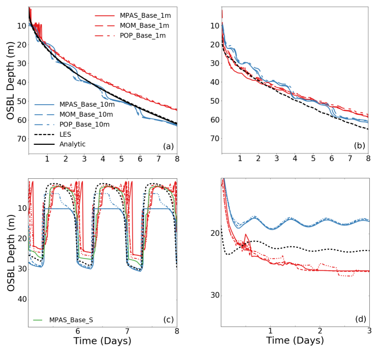
Figure 3: Boundary layer depths computed using equation (8) from the base configuration of MPAS-O, MOM, and POP. (a) Free Convection (FC) test, (b) Convection, Evaporation, and Wind (CEW) test, (c) Diurnal Cycle (DC) test, and (d) Heating and Wind (HW) test. In each panel, the LES output is dashed black and in (a) the thick black line is an analytic solution computed from equation (64).

4.2 Exhibiting sensitivity to vertical grid resolution

A number of the test cases (e.g. FC and DC) show that, surprisingly, the KPP boundary layer depth is more consistent with LES at coarser resolution. In contrast, the finer grid resolution simulations exhibit a persistent shallow boundary layer bias. As an example, Figures 3a and c illustrate a persistent shallow bias in OSBL depths at high resolution relative to LES and coarse resolution KPP results.

To further quantify the resolution dependent bias, we have examined two additional vertical grids: d$z=20$m in the FC and FCML (free convection, mixed layer) tests and a non-uniform grid with 1.5 m resolution near the surface (tagged S in Figures 3 and 6) in the diurnal cycle (DC) test. Such non-uniform grid spacing is commonly used in realistic climate models. The resulting OSBL depths are shown in Figure 6. In the FC and FCML tests and during times of destabilizing surface buoyancy in the DC test there is a persistent shallow bias at the finest grid spacing. As the grid spacing coarsens, the OSBL deepens. When d$z=20$m the OSBL is deeper than LES (Figure 6a and e), suggesting that the minimal bias seen for d$z=10$m in the FC and FCML tests is fortuitous.

At the two finer resolutions (d$z=1$m and stretched grid), high frequency temporal OSBL noise develops near the surface boundary during stabilizing buoyancy forcing (e.g., Figure 6b) in the DC test case. This behavior is similar to what is seen in the FC test (Figure 6a, near the start of the simulation). The noise at high, near surface resolution, and the deep bias for coarse resolution suggests that the enhanced diffusivity parameterization is an incomplete representation of unresolved entrainment across resolutions and surface forcing. We examine these biases in more detail and present a possible solution in Section 5.3.

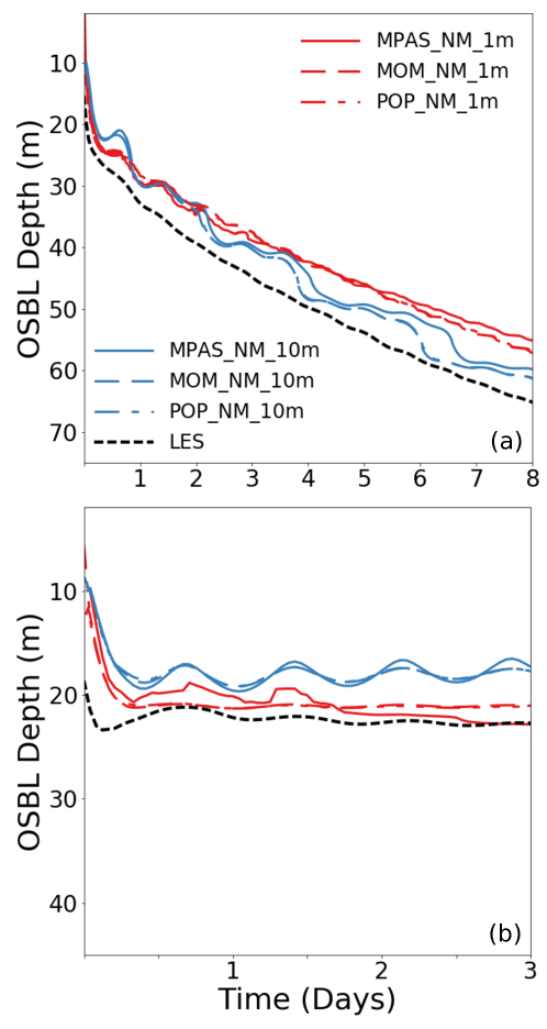
Figure 4: As in Figure 3 but for the no internal match configuration. (a) CEW test and (b) HW test. The FC and DC tests are not shown as there is no predicted internal mixing and thus the solutions are identical for the baseline and no match configurations.

4.3 Sensitivity to time step

The WNF (wind stress with no Coriolis) test has been used as a benchmark for one-dimensional turbulence models (e.g., Burchard and Bolding, 2001). It is motivated by the laboratory experiment conducted by Kato and Phillips (1969), who measured the deepening of the surface boundary layer in an initial linearly stratified fluid ($N^{2}=10^{-4}s^{-2}$) forced by a constant surface friction velocity ($u_{*}=0.01ms^{-1}$).

The boundary layer depth in the experiment is defined as the depth of the maximum $N^{2}$ in the water column. We refer to this as the Kato Phillips (KP) boundary layer depth ($h_{\mbox{\tiny KP}}$). Kato and Phillips (1969) found that the KP boundary layer depth followed an empirical relation given by

$$h_{\mbox{\tiny KP}}=\frac{1.05\,u_{*}\,\sqrt[]{t}}{\sqrt[]{N(t=0)}}.$$ (27)

The WNF test is run for 24 hours as Kato and Phillips (1969) found this relation to only be valid for timescales on the order of 30 hours.

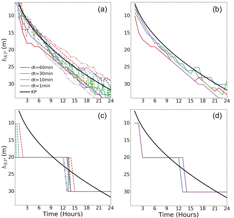
Figure 5: Test Case WNF: Evolution of $h_{\mbox{\tiny KP}}$, defined in equation (27). (a) Base configuration – d$z=1$m, (b) No match configuration with d$z=1$m, (c) Base configuration – d$z=10$m, and (d) No match configuration – d$z=10$m. In every plot, the colors represent the time step size in minutes (see legend in (a)). The black line in all plots is given by equation (27). In the base configuration, the solid lines are MPAS results, the dashed line are MOM6 results, and the dot-dashed lines are POP results. See Section 5.2 for discussion of the no matching approach.

Figure 5 shows the simulated $h_{\mbox{\tiny KP}}$ for the base (a and c) and the no match case (b and d) configurations of KPP. At fine resolution and across all timesteps tested, KPP (in both configurations) well captures the empirical relation given in equation (27). Coarse resolution simulations also perform reasonably well. Consistent with Section 4.2, there are only minor differences between MPAS and MOM6 results. We attribute the noise in Figure 5a to the algorithm we use to diagnose $h_{\mbox{\tiny KP}}$. In particular, we did not interpolate between levels. Rather, the algorithm simply returns the level of maximum stratification in the column. Our results show that KPP is robust with respect to the chosen time step.

5 Treatment of the boundary layer base

The KPP diagnosed OSBL depth is a critical parameter in the predicted vertical turbulent flux (e.g. equations (5) and (6)). The diagnosed boundary layer depth is dependent on the near surface processes through the surface layer buoyancy and momentum (equation (8)) and processes near the boundary layer base. Here we examine KPP sensitivities to the parameterization of entrainment and diffusivity near the boundary layer base.

5.1 Remedies for the shallow bias with fine grid spacing

We revisit how the boundary layer depth is diagnosed as a means to help understand the shallow bias seen in the fine-resolution KPP simulations. For simplicity, focus on the FC and DC tests, in which the KPP boundary layer depth computed according to equation (8) simplifies to

$$Ri_{\mbox{\tiny crit}}=\frac{h\,\left[b_{\tiny\mbox{sl}}-b(h)\right]}{C\,h\,N_{osbl}\,w_{*}}.$$ (28)

To reach this expression, we made use of a simplified definition of the unresolved shear, $V_{t}^{2}$, in which all the constants in equation (17) are subsumed into $C$, and we further assume zero velocity. Hence, for a fixed boundary layer buoyancy, $b_{\tiny\mbox{sl}}$, and surface buoyancy forcing, which fixes $w_{*}$, the key means to modify the Richardson number and hence deepen the boundary layer ($h$) in equation (28) is via the stratification near the OSBL base as measured by $N_{osbl}$.

5.1.1 Sensitivity of the Bulk Richardson number to $N_{osbl}$

Increased stratification near the OSBL base increases the unresolved turbulent shear, $V_{t}^{2}$ (equation (17)). This increased $V_{t}^{2}$ in turn reduces the bulk Richardson number. The diagnosed boundary layer depth then increases to further enhance mixing. At fine vertical resolution, the stratification varies rapidly in the entrainment layer, which is a region of large stratification (e.g., the region near $d/h=1$ in Figure 2). These features of the boundary layer and the adjacent interior suggest that the KPP boundary layer depth can be very sensitive to the chosen level of stratification used for computing $V_{t}^{2}$.

Danabasoglu et al. (2006) define $N_{osbl}$ for the Richardson number calculation according to

$$N_{osbl}=\frac{b(k_{osbl+1/2})-b(k_{osbl-1/2})}{z(k_{osbl+1/2})-z(k_{osbl-1/2})},$$ (29)

where $k_{osbl}$ is the vertical index for the grid cell closest to the OSBL depth. Yet, as shown in Section 2.5.1, the chosen $N_{osbl}$ should be defined one cell shallower in the column, i.e.,

$$N_{osbl}=\frac{b(k_{osbl-1/2})-b(k_{osbl-3/2})}{z(k_{osbl-1/2})-z(k_{osbl-3/2})}.$$ (30)

Test Name	$V_{t}^{2}(h)_{orig}\,(m^{2}s^{-2})$	$V_{t}^{2}(h)_{new}\,(m^{2}s^{-2})$
FC_1m	0.0147	0.0225
FC_10m	0.0173	0.0170
CEW_1m	0.0129	0.0192
CEW_10m	0.0124	0.0139
FCML_1m	0.0354	0.0223
FCML_10m	0.0094	0.0148
HW_1m	0.0112	0.0042
HW_10m	0.0055	0.0039
DC_1m	$1.50\times 10^{-3}$	$1.88\times 10^{-3}$
DC_10m	$2.17\times 10^{-3}$	$1.50\times 10^{-3}$

Table 7: Influence of alteration of $N_{osbl}$ on $V_{t}^{2}$. The subscript $orig$ defines $N_{osbl}$ via equation (29) and subscript $new$ uses equation (30). The 1m and 10m tags specify the vertical resolution. All values are averaged over the last day of the simulation.

Table 7 shows the influence of changing the definition of $N_{osbl}$. The middle column defines $N_{osbl}$ via equation (29) and the third column uses equation (30). Tests and resolutions where $V_{t_{new}}^{2}$ is larger than $V_{t_{orig}}^{2}$ will exhibit deeper boundary layers (assuming identical surface forcing). As expected, the influence of $N_{osbl}$ is smaller for coarser resolution as the entrainment layer is not well resolved. Note that in many of the tests, the diagnosed value of $V_{t}^{2}$ decreases when $N_{osbl}$ is defined by equation (30), which would result in shallower boundary layers.

5.1.2 Modifying $N_{osbl}$ to reduce the shallow bias

The above considerations suggest equation (30) is not optimal. It is also not robust since it can, particularly at coarse resolution, lead to $N_{osbl}\approx 0$ which leads to a non-robust calculation of the Richardson number.

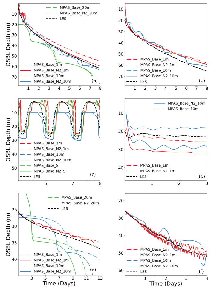
Figure 6: KPP sensitivity to the chosen level of stratification in equation (17). In all panels, the base configuration result is reproduced as the dashed lines. The solid lines are for tests using equation (31) and are tagged N2. (a) FC test, (b) CEW test, (c) DC test, (d) HW test, (e) FCML test, and (f) CWB test. In all plots, the boundary layer depths are computed using equation (8)

Our tests suggest the following more preferable alternative given by

$$N_{osbl}=\max\left(\frac{b(k_{osbl+1/2})-b(k_{osbl-1/2})}{z(k_{osbl+1/2})-z(k_{osbl-1/2})},\frac{b(k_{osbl-1/2})-b(k_{osbl-3/2})}{z(k_{osbl-1/2})-z(k_{osbl-3/2})}\right).$$ (31)

In Figure 6, we exhibit OSBL depths from a series of tests using equation (31) for the $V_{t}^{2}$ calculation. The new definition of $N_{osbl}$ greatly reduces the shallow bias found at fine resolution in the FC test (Figure 6a). The coarse resolution (d$z=10$m and d$z=20$m) FC result is nearly unchanged from the base case, since the entrainment layer is strongly smoothed at coarse resolution and the stratification is constant below the boundary layer.

In the CEW and CWB tests, the model-predicted shear of horizontal momentum dominates the denominator of Equation (8), minimizing the influence of $V_{t}^{2}$ and hence $N_{osbl}$ (Figures 6b and f).

In the DC test, the new calculation of $N_{osbl}$ again slightly diminishes the resolution dependent bias during destabilizing surface buoyancy forcing (Figure 6c). In the DC test we again present results from a non-uniform vertical resolution. The influence of altering $N_{osbl}$ is weaker at this resolution and continues to weaken as the resolution coarsens. Yet, unlike the FC test, the near-surface noise remains (compare Figures 6a and c).

Under stabilizing surface forcing (the HW test), altering $N_{osbl}$ deepens the OSBL significantly. The shallow OSBL bias at coarse resolution is now a deep bias. The slight OSBL deep bias increases at high resolution.

In the FCML test (Figure 6e) the boundary layer is roughly unchanged when equation (31) is used in the $V_{t}^{2}$ parameterization. Altering the definition of $N_{osbl}$ at coarse resolution has a larger impact on the KPP simulated OSBL. The dependence of KPP on $V_{t}^{2}$ at coarse resolution was not seen in most tests (Figure 6). We believe that the coarse resolution KPP is more sensitive to the $V_{t}^{2}$ parameterization in the FCML test due to the very strong stratification near the base of the OSBL.

In most cases, altering the definition of $N_{osbl}$ reduces OSBL bias relative to LES, although slightly. In the FCML and HW tests the OSBL bias increases. Our results suggest that altering $N_{osbl}$ is a useful, but not critical consideration for KPP configurations.

5.2 Diffusivity at the boundary layer base

As discussed in Section 2.4, there are a number of important considerations regarding the internal matching scheme of KPP. Our results suggest that the base and no match configurations, with a few critical alterations, can perform well relative to LES.

5.2.1 Considerations for the no-match configuration

In the convection, evaporation, and wind (CEW) and heating and wind (HW) tests, the OSBLs depth from the no match (NM) configuration are shallower than the base configuration of KPP (compare Figures 3b and d to Figure 4). We suggest that the shallow OSBL bias in the NM configuration is partially caused by the inability of shear instability mixing to influence the OSBL (consistent with LMD94). Figure 7 shows the influence of extending the LMD94 shear instability mixing scheme into the OSBL (NM_Add test) for the three tests that are wind forced. At high resolution, the OSBL depths increase when shear instability mixing is included in the OSBL, decreasing the bias relative to LES.

In the convection, wind, background shear (CWB) test, which simulates a boundary layer deepening into a region of preexisting shear, the OSBL bias increases. Temporal noise also develops.

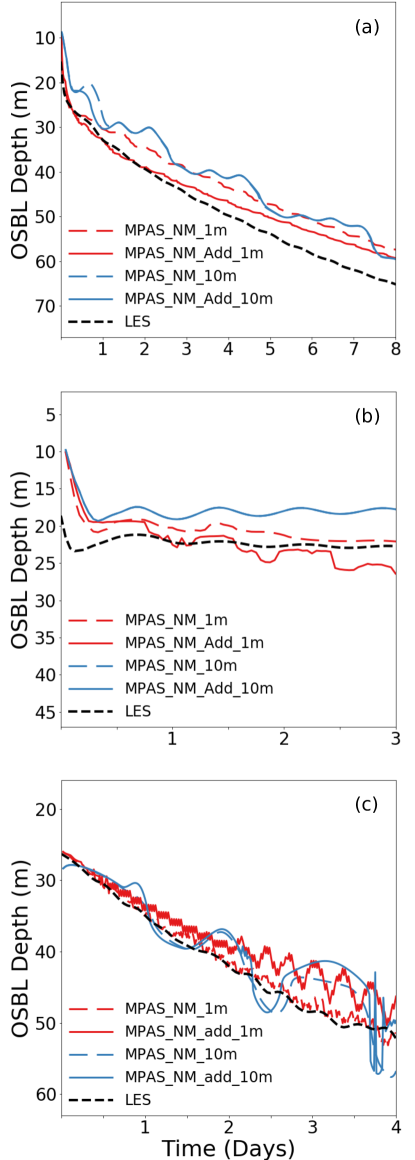
Figure 7: OSBL depths from tests examining the sensitivity of adding shear instability mixing in the boundary layer when diffusivity matching is disabled. (a) CEW test, (b) HW test, and (c) CWB test. In every test, the boundary layer depth is calculated following equation (8).

At coarse resolution, the inclusion of shear instability mixing in the OSBL does not dramatically alter the results. It is likely that the insensitivity to interior mixing in the OSBL is due to the weakened modeled vertical shear of horizontal currents and buoyancy gradients resulting from a larger d$z$.

Overall, KPP simulations with the NM configuration are similar to the base configuration. Adding diffusivities from interior mixing schemes (e.g., shear instability) can slightly reduce biases in a few cases (e.g. HW and CEW), but can increase temporal noise in the simulated OSBL. Therefore, in the no-match configuration we do not recommend adding diffusivities from the shear instability scheme to the KPP diagnosed value in the no-match configuration.

Finally we note that even though OSBL depths simulated by the no-match configuration are similar to the baseline configuration, the no-match configuration does not require the complexities associated with matching viscosities and diffusivities between the KPP scheme and internal mixing parameterizations.

5.2.2 Considerations for the base configuration

Recall that the CVMix base configuration of KPP does not match to gradients of internal diffusivities, which is different from LMD94 and Danabasoglu et al. (2006). Sensitivity to this choice is tested in Figure 8. In the CEW test there is minimal sensitivity to the matching of internal diffusivity gradients. However, in the HW test (Figure 8b), matching to internal diffusivity gradients increases the OSBL bias relative to LES at high resolution.

In the CWB test, the MB (matching diffusivity and the gradient from internal mixing) test result in brief periods of anomalously strong momentum fluxes (e.g., near day 3 in Figure 9b). When the OSBL deepens into the layer of strong background shear, the interior predicted diffusivities can vary rapidly near the OSBL base and thus strongly influence the KPP OSBL diffusivities. When we match to the interior predicted diffusivities and viscosities alone (CVMix default), these regions of vigorous fluxes are strongly damped (compare Figures 9b and c).

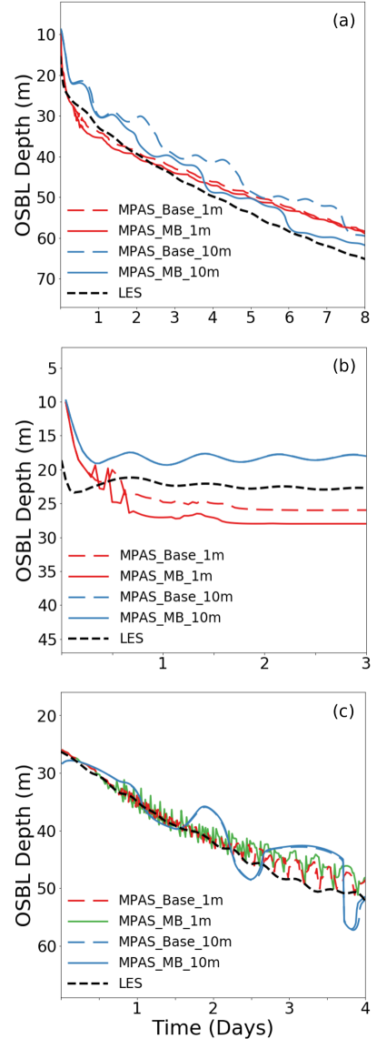
Figure 8: As in Figure 7 but for sensitivity tests matching the gradient of internal diffusivities.

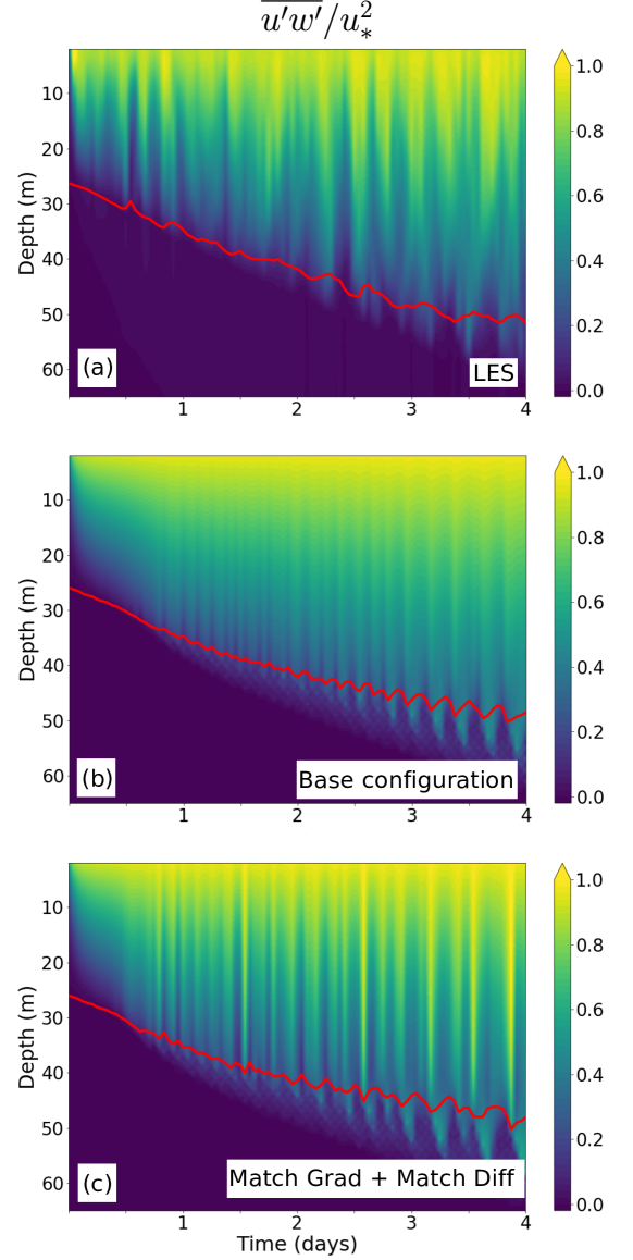
Figure 9: Test Case CWB: Turbulent momentum flux normalized by the surface friction velocity (a-c). The LES results are the top row, the middle row is the base configuration and the bottom row is a test where matching is to the internal diffusivity alone. For KPP simulations, the turbulent fluxes are computed via the parameterizations in Equations (5), (6), and (19). In every plot, the red line is the boundary layer depth computed via Equation (8).

Our results (in particular the CWB test) suggest that if internal matching is used, matching should be to internal diffusivities only and not the gradient.

5.3 Property exchange across the OSBL base

KPP models entrainment buoyancy fluxes via:

• the model-resolved vertical shear of horizontal currents

• the unresolved turbulent shear ($V_{t}^{2}$) parameterization,

• and the enhanced diffusivity parameterization.

The first two methods directly alter the boundary layer depth via equation (8). As the resolved shear of horizontal currents and unresolved turbulent shear increase, the bulk Richardson number decreases, deepening the boundary layer. A deeper boundary layer increases the entrainment buoyancy flux.

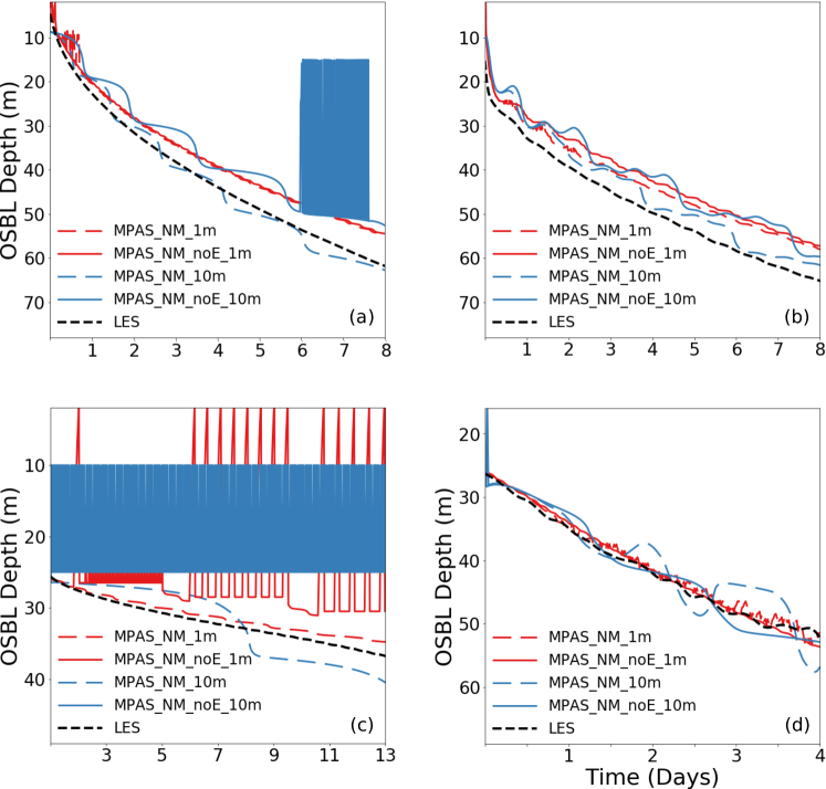
Figure 10: Boundary layer depth sensitivity to the enhanced diffusivity parameterization in the no matching configuration. The LES output is dashed black. The baseline configuration results are reproduced as dashed lines. All OSBL depths are computed using Equations (8). (a) The FC test, (b) the CEW test, (c) the FCML test, and (d) the CWB test.

LMD94 describe the enhanced diffusivity parameterization as a method to overcome a shallow bias and boundary layer ”stair case” structures at coarse resolution. This suggests that the enhanced diffusivity parameterization attempts to represent unresolved sources of entrainment. Yet our tests show that the enhanced diffusivity parameterization can lead to strong resolution dependence in simulated boundary layer depths. Figure 10 shows boundary layer depths for tests without the enhanced diffusivity parameterization. In test cases with small vertical shear of resolved horizontal momentum (e.g. a-c) the coarse resolution OSBL depth shallows when the enhanced diffusivity parameterization is disabled. Note that while the OSBL depth bias relative to LES increases, the KPP resolution dependence is diminished (Figure 10a and b especially)

To examine the resolution dependent bias in more detail, Figure 11 shows the time averaged entrainment flux across a wide range of vertical grid spacings (d$z=0.1$m - d$z=20$m) for four test cases (FC, CEW, FCML, and CWB). In the FC, CEW, and FCML cases the entrainment buoyancy flux simulated by the base configuration is strongly dependent on resolution (black circles). In the CWB test, there is minimal variation due to the large imposed background shear.

If the enhanced diffusivity parameterization is disabled, the entrainment buoyancy flux is strongly reduced in Figures 11a-c. This further demonstrates that the enhanced diffusivity parameterization seeks to represent unresolved sources of entrainment.

The weak entrainment when enhanced diffusivity is disabled leads to large temporal noise in the FC and FCML test cases (Figures 10a and c). Recall that the non-local tracer flux (equation (18)) causes cooling near the OSBL base in the presence of surface cooling via a redistribution of the surface flux. Without sufficient entrainment, static instability can develop near the OSBL base. When $N^{2}<0$, the unresolved turbulent shear is assumed to be zero. This increases the bulk Richardson number (equation (8)), which shallows the OSBL.

These large oscillations are evident in similar MOM6 and POP configurations as well (not shown). While the mean deepening of the OSBL remains consistent in many cases even without sufficient entrainment, we note that the rapidly oscillating OSBL depths could have strong interactions with other parameterizations (e.g., symmetric instability, Bachman et al., 2017).

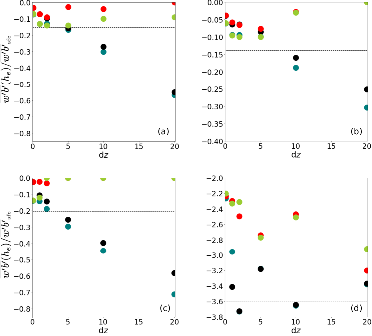
Figure 11: Time averaged (over last day of simulation) entrainment buoyancy flux, which is defined as the minimum buoyancy flux in the profile, normalized by the surface buoyancy flux. The entrainment buoyancy flux is shown as a function of KPP resolution. The black circles include the enhanced diffusivity parameterization and the red circles do not. The yellow-green circles include the alteration to $V_{t}^{2}$ but disables the enhanced diffusivity parameterization and the teal circles include both changes. The LES entrainment buoyancy flux is shown as the horizontal dashed black line in each figure. (a) The FC test, (b) the CEW test, (c) the FCML test, and (d) the CWB test.

If the definition of $N_{osbl}$ is altered (equation (31)), the entrainment buoyancy flux increases in the base configuration (teal circles, Figure 11) as expected. If the enhanced diffusivity parameterization is disabled in addition to altering $N_{osbl}$ (yellow-green circles, Figure 11) the resolution dependence is reduced, although the entrainment flux is too weak. These results suggest that the enhanced diffusivity parameterization leads to the observed resolution dependence for KPP simulated OSBL depths (Figure 3). However, the enhanced diffusivity parameterization is necessary to provide sufficient entrainment in order to prevent temporal noise in OSBL depths. We discuss this issue further in light of the non-local tracer transport parameterization in the next section.

6 Non-local transport in KPP

We focus in this section on the parameterized non-local tracer transport from KPP. The non-local transport is enabled only for destabilizing surface buoyancy forcing. Across most test cases, the KPP non-local transport parameterization behaves well. Yet our experiments also suggest possibilities for extensions worthy of further research.

6.1 Tracer transport

FC sensitivity tests show that if entrainment is not predicted correctly (i.e., too weak), the OSBL oscillates rapidly due to an interaction with the non-local temperature flux parameterization. This bias is mitigated by the enhanced diffusivity parameterization. However, for shallow OSBL depths at high resolution, temporal noise is evident even with the enhanced diffusivity parameterization enabled (Figure 3a).

In the DC test we examined the sensitivity of the non-local temperature flux (equation (18)) to the amount of shortwave radiation included in the surface flux. We varied the amount of shortwave radiation in the surface flux from that absorbed in the top layer to that absorbed in the entire OSBL. Across these tests, we found very little variation in the simulated OSBL depths (not shown). This is consistent with LMD94 (see their Figure C4, Appendix C) as this study and LMD94 use an equation of state where density increases until freezing occurs (e.g., equation (22)).

In KPP, the non-local tracer transport derives from the buoyant production term in the turbulent flux equation (e.g. equation (20)) and is only non-zero in the presence of a non-zero surface tracer flux. In the FCML test there is no non-local salinity transport even though there is a destabilizing buoyancy flux.

To examine this assumption, we show the salinity flux budget tendency terms in equation (32) from the FCML LES test case in Figure 12, where the two panels span the entire boundary layer, but the x-range in the upper OSBL is tightened to better elucidate the profiles. Note that the sum of the tendency terms in Figure 12 is not exactly zero, most likely due to the lack of inclusion of subgridscale turbulent flux tendencies in Equation (32) (Mironov, 2001).

$$\frac{\partial\overline{w^{\prime}S^{\prime}}}{\partial t}=-\underbrace{\overline{w^{\prime^{2}}}\frac{\partial\overline{S}}{\partial z}}_{\textrm{local}}+\underbrace{g\left(\alpha_{\theta}\overline{\theta^{\prime}S^{\prime}}-\beta_{S}\overline{S^{\prime^{2}}}\right)}_{\textrm{buoyancy}}-\underbrace{\frac{\partial\overline{w^{\prime}w^{\prime}S^{\prime}}}{\partial z}}_{\textrm{triple moment}}-\underbrace{\overline{\frac{S^{\prime}}{\rho_{o}}\frac{\partial p^{\prime}}{\partial z}}}_{\begin{subarray}{c}\textrm{pressure-salinity}\\ \textrm{covariance}\end{subarray}}.$$ (32)

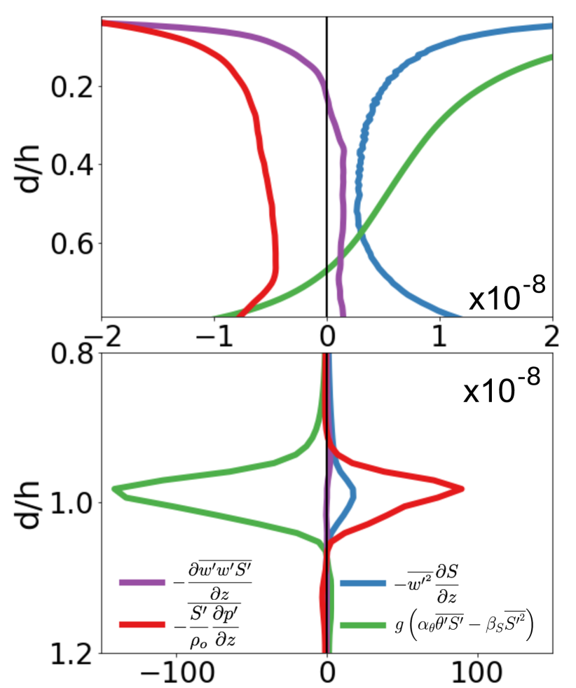
Figure 12: Test Case FCML: budget terms for the turbulent salinity flux equation (see Equation (32)) diagnosed from LES. The red line is the pressure-salinity covariance, the green line is the buoyant production term, the blue line is the local production term, and the purple line is the triple moment term. All data has been averaged over the final 12 hours of day 12.

Figure 12 shows that the buoyant production of the turbulent salinity flux (recall the non-local transport in KPP derives from this term) is larger in magnitude to the local production of the turbulent salinity flux in the OSBL. The non-zero non-local production of the turbulent salinity flux in the FCML test implies that the KPP formulation of non-local tracer transport is incomplete. Indeed, Noh et al. (2003) show that inclusion of a non-local redistribution of the entrainment heat flux results in a reduced bias for an atmospheric vertical mixing parameterization similar to KPP relative to an atmospheric LES. A parameterization similar to Noh et al. (2003) could replace the enhanced diffusivity parameterization of LMD94 and perhaps reduce the resolution dependence seen in predicted OSBL depths given there is no explicit consideration of grid resolution in the Noh et al. (2003) parameterization.

6.2 Momentum transport

Figure 13 shows the zonal and meridional momentum fluxes for the CEW test. The base configuration is shown for MPAS-O, MOM6, and POP. In every model, the KPP simulated zonal momentum flux matches LES fairly well (Figure 13a). However, the KPP predicted meridional momentum flux profile is much too strong through much of the OSBL (Figure 13b). The vigorous LES meridional momentum flux in the presence of minimal velocity gradient (Figure 13d) suggests an important role for non-local momentum transport. The lack of a non-local momentum transport could explain the OSBL shallow bias seen in the CEW test (Figure 3b).

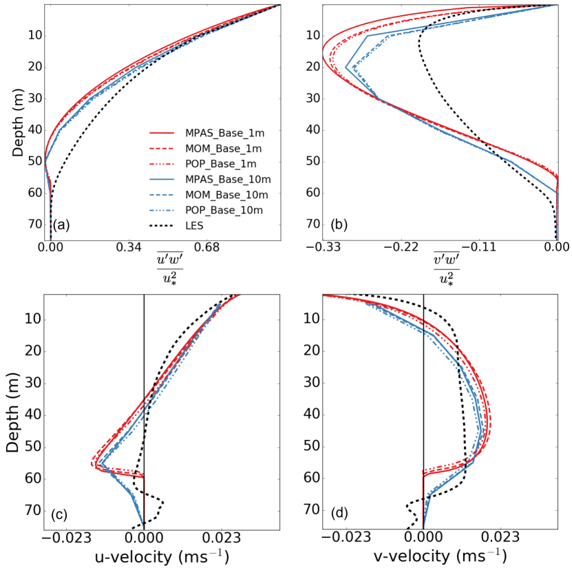
Figure 13: Test Case CEW: time averaged, normalized momentum flux: (a) zonal momentum flux ($\overline{u^{\prime}w^{\prime}}$), (b) meridional momentum flux ($\overline{v^{\prime}w^{\prime}}$), (c) zonal velocity, and (d) meridional velocity. The KPP momentum fluxes are computed via the parameterizations in Equations (5), (6), and (19). The line colors are defined in Figure 3. All profiles have been averaged over day 8.

7 Conclusions and recommendations

In this paper, we investigated the behavior of the KPP boundary layer parameterization as implemented within the CVMix package (Griffies et al., 2015). The KPP scheme was rigorously tested against a series of horizontally averaged LES. Further, in each case, we also varied $\mbox{Ri}_{\mbox{\tiny crit}}$. When $\mbox{Ri}_{\mbox{\tiny crit}}$ was increased, the boundary layer did deepen, but not linearly due to $V_{t}^{2}$.

While many different implementations of KPP have been tested in a number of circumstances; e.g., observations ((e.g., LMD94, Zedler et al., 2002; Van Roekel and Maloney, 2012; Mukherjee and Tandon, 2016), large-scale ocean simulations (e.g., Li et al., 2001), and against limited LES (e.g., Large and Gent, 1999; McWilliams and Sullivan, 2000; Smyth et al., 2002; Noh et al., 2016; Reichl et al., 2016), it has not been subject to testing against a series of tightly controlled LES cases. These tests focused on implementation choices related to vertical physics alone under simplified surface forcing. The tests presented here do not consider the influence of horizontal processes. This is an important and active (Bachman et al., 2017) direction for future evaluation of KPP.

Our tests have focused on four main components of KPP physics and numerical choices: vertical resolution and timestepping (Sections 2.7 and 4), internal matching (Sections 2.4 and 5.2), entrainment at the OSBL base (Sections 2.5 and 5.3), and non-local transport (Sections 2.6 and 6). The key findings from the most critical areas and a few potential solutions are summarized below

• Model Choices:

  • The CVMix implementation appears robust across calling models as three very different calling models gave similar results (Section 4).

  • KPP is sensitive to the vertical resolution chosen (Section 4.2). Using Equation (31) in the $V_{t}^{2}$ parameterization mitigates some of this resolution-dependent bias (e.g., Figure 6 and 11).

  • KPP is robust to variation in model timestep (Figure 5).

• Non-local transport:

  • The results of the FCML test case suggest that a non-local transport based on surface fluxes alone is not sufficient (Figure 12) and a non-local redistribution of the entrainment buoyancy flux should be explored.

  • Results of the CEW and CWB tests (Figure 13) suggest that a non-local momentum transport parameterization is a critical need for KPP (Section 8.1).

• Treatment at the Boundary Layer Base:

  • It has been suggested (LMD94) that $\mbox{Ri}_{\mbox{\tiny crit}}$ should vary with vertical resolution and previously proposed functions of $\mbox{Ri}_{\mbox{\tiny crit}}(dz)$ were found by matching to d$z=1$m results. However, determining the correct form of $\mbox{Ri}_{\mbox{\tiny crit}}(dz)$ is further complicated for models with non-uniform vertical resolution (e.g., MPAS-O). For simplicity, it is recommended to choose a single value of $\mbox{Ri}_{\mbox{\tiny crit}}$ across most resolutions.

  • KPP simulates entrainment buoyancy fluxes in two ways. At high resolution, the entrainment fluxes are very sensitive to the $V_{t}^{2}$ parameterization. Use of Equation (31) in the $V_{t}^{2}$ parameterization reduces this sensitivity. At coarse resolution, entrainment strength is determined by the enhanced diffusivity parameterization. In a number of tests this parameterization caused a bias that grew with resolution (Figure 6).

  • For shallow boundary layers and at high resolution (e.g., the DC test case), high frequency OSBL depth noise develops (Figure 3c). This suggests a lack of simulated entrainment within KPP for this test case.

  • KPP OSBL biases relative to LES are similar for configurations with and without matching to interior diffusivities (compare Figures 3b and d to Figure 4). Our results suggest considerations for both configurations of KPP (base and no match) that are summarized below:

    • Matching to interior mixing: Matching to the internal diffusivity and its vertical gradient can lead to noise in the simulated OSBL depths (Figure 8) and periods of anomalously strong fluxes (Figure 9. Therefore, if matching is retained we recommend matching to the internal diffusivity only and not its gradient.

    • No matching: diffusivities and viscosities from the LMD94 shear instability parameterization should not be considered in the OSBL. Including interior diffusivities in the OSBL reduces the OSBL depth bias slightly in two test cases (CEW and HW, Figures 7a-b), but introduces temporal oscillations in the OSBL depth in the CWB test case (Figure 7c)

8 Future work

In addition to proposed modifications to the baseline configuration KPP and a new configuration that does not match to internal predicted diffusivities/viscosities, the results also suggest directions for future improvements to KPP.

8.1 Non-local transport

Results of the FCML test case suggest that assuming the non-local flux redistributes the surface flux alone is not complete. There is an equally large contribution from non-local processes throughout the OSBL in the absence of surface fluxes in the FCML test (see Figure 12). Thus the current implementation for non-local tracer fluxes in KPP must be extended. Including a separate parameterization for non-local entrainment fluxes (similar to Noh et al., 2003) may be a viable path forward.

In the CEW test, the meridional momentum profiles in LES were well mixed in the middle of the OSBL, whereas in KPP a strong gradient exists (Figure 13d). The meridional momentum flux for LES and KPP is strong in the OSBL (Figure 13c). The presence of a meridional momentum flux in the presence of minimal vertical gradients of meridional momentum suggest an importance of non-local momentum transport.

We see two possible paths for the inclusion of non-local momentum transport in KPP. First, we could use the form suggested by Smyth et al. (2002). To the best of our knowledge, this parameterization has not been tested outside of Smyth et al. (2002) even though it is based on some theoretical considerations and a similar parameterization has been tested in atmospheric LES (Frech and Mahrt, 1995; Brown and Grant, 1997). Thus the Smyth et al. (2002) parameterization is not yet recommended for inclusion in CVMix.

Alternatively, we could derive an explicit equation for the momentum flux following Donaldson (1972). To make the equation tractable, we could also assume that any product of perturbations involving horizontal quantities (e.g., $u^{\prime}$) alone and products involving the Coriolis parameter ($f$) are negligible. If we use the pressure strain correlation closure of Canuto et al. (2007), we can write an equation for the turbulent vertical flux of zonal momentum as,

$$\overline{u^{\prime}w^{\prime}}\approx-\tau\overline{w^{\prime^{2}}}\left(\frac{\partial\overline{U}}{\partial z}-\frac{1}{\overline{w^{\prime^{2}}}}\frac{\partial\overline{u^{\prime}w^{\prime^{2}}}}{\partial z}-\frac{C_{1}\overline{u^{\prime}b^{\prime}}}{\overline{w^{\prime^{2}}}}\right).$$ (33)

Here, $\overline{u^{\prime}b^{\prime}}$ is the horizontal buoyancy flux, and $C_{1}$ is a constant. If we ignored the horizontal buoyancy flux, we could perhaps follow HM91 to derive a closure for non-local momentum transport. Yet, Holtslag and Moeng (1991) considered free convective conditions and thus the potential application to a non-local momentum parameterization is tenuous. Additional LES cases must be considered to determine how to appropriately parameterize the second and third terms in Equation (33).

Within a possible non-local momentum transport it is important to include enhancement due to Langmuir turbulence. Previous work (McWilliams and Sullivan, 2000; Li et al., 2015; Reichl et al., 2016) have suggested parameterizations for the influence of Langmuir turbulence on the local diffusivity in KPP, but a non-local momentum parameterization that includes Langmuir turbulence has not been proposed. It is possible that previously derived vertical velocity scalings (e.g., McWilliams and Sullivan, 2000; Van Roekel et al., 2012) could be used to derive a modified convective velocity scale for a new non-local momentum flux parameterization following the equation (33) or to modify the non-local momentum flux proposed by Smyth et al. (2002) that includes Langmuir turbulence.

8.2 Amount of incident shortwave radiation transported by the non-local parameterization

As suggested by LMD94, the upper limit for the shortwave contribution to the non-local vertical heat flux is the amount of radiation absorbed in the OSBL. A simple gedanken experiment can demonstrate a pitfall to choosing this upper bound in models with penetrating shortwave radiation. Assume brackish surface waters, with a SST below the temperature of maximum density. Further assume that local vertical mixing is small and shortwave radiation is the only heat flux. Finally assume a deep OSBL. In this circumstance solar heating leads to an unstable OSBL, and thus the non-local parameterization is active. With a deep OSBL, all of the incident shortwave radiation is included in the non-local tracer transport, which results in a solar heat flux and non-local heat flux that exceeds the surface heat flux. Thus new cold water masses would be generated near the surface that were not present in the water column. In a more realistic configuration, this could lead to the artificial generation of sea ice.

A possible solution is to make the strength of the non-local flux depth dependent and to only include the portion of the shortwave radiation that is absorbed between the sea surface and a given depth in the non-local temperature transport. This ensures that the redistributed heat flux is smaller than the total shortwave radiation entering the ocean. Testing this solution and determining the appropriate amount of shortwave radiation to include in the non-local tracer transport would require modifications to the buoyancy equation and subgrid TKE schemes in the LES model.

8.3 OSBL entrainment

To reduce the dependence of the entrainment flux across resolutions and forcing we could follow the suggestion of Noh et al. (2003), who suggest an explicit parameterization for the entrainment heat flux, including a non-local redistribution of this flux. In KPP the vertical entrainment heat flux is artificially separated from the remainder of the OSBL turbulent flux (and slaved to the OSBL depth prediction). A parameterization for an entrainment heat flux similar to Noh et al. (2003) would make the boundary layer depth a diagnostic variable with no feedbacks into the scheme. A diagnostic OSBL depth could eliminate mixing sensitivity to $V_{t}^{2}$ and the enhanced diffusivity parameterization in KPP.

In summary, the current configuration of KPP has performed well in many scenarios. However, alternative approaches or extensions to KPP are needed to improve model fidelity for several relevant dynamic and thermodynamic situations. Research into these challenging areas is underway.

Appendix A Elements of the KPP boundary layer scheme

For any prognostic scalar or vector field component $\psi$ (e.g., velocity components, tracer concentrations), the KPP scheme parameterizes the turbulent vertical flux within the surface boundary layer according to

$$\overline{w^{\prime}\psi^{\prime}}=-K_{\psi}\left(\frac{\partial\psi}{\partial z}-\gamma_{\psi}\right).$$ (34)

In this equation, the eddy diffusivity $K_{\psi}$ is written as the product of three terms

$$K_{\psi}=h\,w_{\psi}\left(\sigma\right)G\left(\sigma\right).$$ (35)

The boundary layer depth $h>0$ scales the diffusivity, so that $K_{\psi}$ is larger for deeper boundary layers. The non-dimensional shape function, $G(\sigma)$, is described in A.1.

The turbulent velocity scale, $w_{\psi}\geq 0$, is computed according to

$$w_{\psi}=\left(\frac{\kappa\,u_{*}}{\phi_{\psi}(\sigma h/L)}\right).$$ (36)

In this expression, $\kappa=0.4$ is the von Kármán constant, $u_{*}\geq 0$ is the friction velocity scale (determined by the square root of the surface stress magnitude), $\sigma$ is the non-dimensional boundary layer coordinate (see equation (3)), and $L$ is the Obukhov length scale, which is held fixed at its surface value. The function $\phi_{\psi}\geq 0$ is a non-dimensional flux profile that is smaller for negative buoyancy forcing and goes to unity in the absence of buoyancy forcing. Given this form, the velocity scale $w_{\psi}$ is larger for unstable surface boundary forcing (i.e., negative buoyancy forcing such as when removing heat or adding salt), as well as for stronger mechanical forcing (i.e., larger friction velocity scale as under strong wind forcing).

The KPP vertical viscosity (used for frictional transfer of momentum in the ocean interior) is specified via a separate dimensionless flux profile through the Prandtl number

$$Pr=\left(\frac{K_{v}}{K_{\psi}}\right)=\left(\frac{\phi_{\psi}}{\phi_{m}}\right).$$ (37)

See Appendix B of LMD94 as well as Griffies et al. (2015) for full details of the non-dimensional flux profile functions $\phi_{\psi}$ and $\phi_{m}$, as well as the Obukhov length scale $L$.

A.1 The non-dimensional shape function

In the KPP diffusivity expression (equation (35)), the non-dimensional shape function, $G(\sigma)$, is assumed to take a polynomial form proposed by O’Brien (1970)

$$G(\sigma)=c_{1}+c_{2}\sigma+c_{3}\sigma^{2}+c_{4}\sigma^{3},$$ (38)

where $c_{1},c_{2},c_{3},c_{4}$ are constants to be specified by the following considerations. First, since the diffusivity, $K_{\psi}$, is assumed to go to zero at the ocean surface,

$$c_{1}=0.$$ (39)

Within the surface layer ($0\leq\sigma\leq\epsilon$) (see Figure 1), we can eliminate the gradient of $\psi$ in equation (34) using Monin-Obukhov similarity theory in the form

$$\frac{\partial\psi}{\partial z}=\left(\frac{\overline{w^{\prime}\psi^{\prime}}_{\mbox{\tiny sfc}}}{\kappa\,z\,u_{*}}\right)\phi_{\psi},$$ (40)

where $\overline{w^{\prime}\psi^{\prime}}_{\mbox{\tiny sfc}}$ is the turbulent boundary flux crossing the ocean surface (e.g., turbulent latent and sensible heat; turbulent tracer flux; turbulent momentum flux). If we combine equations (34) and (35) and assume positive surface buoyancy forcing so that the non-local term vanishes ($\gamma_{\psi}=0$) we have

$$\overline{w^{\prime}\psi^{\prime}}=-h\,G\,w_{\psi}\left(\frac{\partial\psi}{\partial z}\right),$$ (41)

which returns us to the KPP closure form assumed in equation (34). Now insert equation (40) into (41), and assume $G(\sigma)\approx\sigma(c_{2}+c_{3}\sigma)$ (valid in the surface layer where $\sigma\leq\epsilon\ll 1$), to yield

$$\overline{w^{\prime}\psi^{\prime}}=-\left(\frac{\overline{w^{\prime}\psi^{\prime}}_{\mbox{\tiny sfc}}}{\kappa\,z\,u_{*}}\right)\phi_{\psi}\,h\,\sigma\,(c_{2}+\sigma c_{3})\,w_{\psi}.$$ (42)

Using equations (36) and (3) brings equation (42) to the form

$$\left(\frac{\overline{w^{\prime}\psi^{\prime}}}{\overline{w^{\prime}\psi^{\prime}}_{\mbox{\tiny sfc}}}\right)=c_{2}+\sigma c_{3}.$$ (43)

Now we assume a linear decrease of the turbulent flux within the surface layer (i.e., $\overline{w^{\prime}\psi^{\prime}}\,\epsilon=\beta\,\overline{w^{\prime}\psi^{\prime}}_{\mbox{\tiny sfc}}$ where $\beta$ is a constant), so that the surface flux at a position $\sigma$ within the surface layer is given by

$$\left(\frac{\overline{w^{\prime}\psi^{\prime}}}{\overline{w^{\prime}\psi^{\prime}}_{\mbox{\tiny sfc}}}\right)=1+\frac{\sigma}{\epsilon}(\beta-1)=c_{2}+\sigma\,c_{3}.$$ (44)

To be valid at $\sigma=0$ requires

$$c_{2}=1.$$ (45)

To determine the final two shape function coefficients, we require matching across the base of the boundary layer, at $\sigma=1$. Use of equation (38) and its derivative at the boundary layer base leads to the following expressions

$$c_{3} =-2+3\,G(1)-\left(\frac{\partial G}{\partial\sigma}\right)_{\sigma=1}$$ (46a)

$$c_{4} =1-2\,G(1)+\left(\frac{\partial G}{\partial\sigma}\right)_{\sigma=1}.$$ (46b)

Thus, the shape function is dependent on the chosen boundary conditions at the base of the OSBL. We next consider these boundary conditions.

A.2 Diffusivity matching for the shape function at the OSBL base

LMD94 suggest that the diffusivity and viscosity predicted by KPP, as well as its vertical derivative, should match that predicted by the sum of all mixing parameterizations in the region below the boundary layer (the ocean interior). To ensure appropriate matching, the necessary inputs to equations (46a) and (46b) are given by

$$G(\sigma) =\frac{K_{\psi}^{\mbox{\tiny INT}}\left(h\right)}{h\,w_{\psi}(\sigma)}$$ (47a)

$$\frac{\partial G}{\partial\sigma} =-\left[\frac{\partial_{z}K_{\psi}^{\mbox{\tiny INT}}\left(h\right)}{w_{\psi}(\sigma)}+\frac{K_{\psi}^{\mbox{\tiny INT}}\left(h\right)\partial_{\sigma}w_{\psi}(\sigma)}{h\,w_{\psi}^{2}(\sigma)}\right],$$ (47b)

where $\partial_{z}$ and $\partial_{\sigma}$ are the partial derivatives with respect to $z$ and $\sigma$ respectively, and we evaluate terms on the right hand side at the boundary layer base, $\sigma=1$. Without diffusivity matching, the shape function takes the relatively simple cubic form used by Troen and Mahrt (1986)

$$G\left(\sigma\right)=\sigma\left(1-\sigma\right)^{2}.$$ (48)

Appendix B Mathematical Symbols

A summary of selected symbols used in this paper, along with their preferred units, are presented in Table 8.

Symbol	Description	units
$\overline{w^{\prime}\theta^{\prime}}_{\mbox{\tiny sfc}}$	surface temperature flux	$\mbox{m}~{}\mbox{s}^{-1}~{}\mbox{K}$
$\overline{w^{\prime}S^{\prime}}_{\mbox{\tiny sfc}}$	surface salinity flux	$\mbox{m}~{}\mbox{s}^{-1}~{}\mbox{ppt}$
$\overline{w^{\prime}b^{\prime}}_{\mbox{\tiny sfc}}$	surface buoyancy flux	$\mbox{m}~{}\mbox{s}^{-1}~{}\mbox{m}~{}\mbox{s}^{-2}$
$h$	ocean boundary layer depth	m
$h_{e}$	depth of the minimum buoyancy flux (entrainment depth)	m
$h_{m}$	depth of the well-mixed layer	m
$\sigma=(-z+\eta)/h$	boundary layer coordinate	non-dimensional
$\epsilon=0.1$	surface layer depth as a percentage of $h$	non-dimensional
$X_{\tiny\mbox{sl}}$	surface layer average of $X$	dimensions of $X$
$G(\sigma)$	shape function for diffusivity profile	non-dimensional
$w_{x}$	turbulent velocity scale of quantity $x$	$\mbox{m}~{}\mbox{s}^{-1}$
$K_{x}$	parameterized KPP eddy diffusivity for quantity $x$	$\mbox{m}^{2}~{}\mbox{s}^{-1}$
$\mbox{Ri}_{\mbox{\tiny b}}$	bulk Richardson number	non-dimensional
$\mbox{Ri}_{\mbox{\tiny crit}}$	critical bulk Richardson number	non-dimensional
$V_{t}^{2}$	squared unresolved turbulent velocity (in $\mbox{Ri}_{\mbox{\tiny b}}$)	$\mbox{m}^{2}~{}\mbox{s}^{-2}$
$\gamma_{x}$	non-local term	$\mbox{tracer conc}~{}*~{}\mbox{m}^{-1}$
$K_{x}\,\gamma_{x}$	non-local flux	$\mbox{tracer conc}~{}*~{}\mbox{m}~{}\mbox{s}^{-1}$
$C_{*}$	strength of non-local term	non-dimensional
$\kappa$	von Kármán constant	non-dimensional
$\alpha_{\theta}$	thermal expansion coefficient	$\mbox{K}^{-1}$
$\beta_{S}$	haline expansion coefficient	$\mbox{ppt}^{-1}$
$\overline{\theta}$	Horizontal mean of temperature	K
$\overline{S}$	horizontal mean of salinity	ppt
$N^{2}\equiv\partial b/\partial z$	squared buoyancy frequency	$\mbox{s}^{-2}$
$\tau$	return to isotropy timescale	s
$g$	gravitational acceleration	$\mbox{m}~{}\mbox{s}^{-2}$
$f$	Coriolis parameter	$\mbox{s}^{-1}$

Table 8: Symbols used in this paper, along with preferred units

Appendix C Salinity testing in the NCAR LES

To simulate the influence of salinity in the NCAR LES model (McWilliams et al., 1997; Sullivan et al., 2007), the influence of salinity on the resolved buoyancy is included via a linear equation of state. Thus the modified buoyancy term in the vertical momentum equation becomes

$$b=-g\left[1-\alpha_{\theta}\left(\theta-\overline{\theta}\right)+\beta_{S}\left(S-\overline{S}\right)\right]$$ (49)

where the overline indicates a horizontal average. Buoyancy terms in the subgrid TKE scheme are modified in a similar fashion. To test this implementation two buoyant bubble tests were conducted. In both tests, the buoyancy perturbation is initialized via

$$b(x,y,z)=min\left[0,\Delta b\;\cos\left(\frac{\pi\,r(x,y,z)}{2}\right)\right]$$ (50)

where $\Delta b$ is the maximum buoyancy perturbation, and $r(x,y,z)$ is the distance from the bubble center. One test is initialized by a temperature perturbation. For the second test, the salinity is initialized such that in buoyancy the perturbation is identical to the temperature test. The results from this test are shown in Figure 14. The thin solid lines are for the temperature perturbation and the thick dashed lines are the salinity perturbations. As the two bubbles have identical buoyancy they should fall on top of each other. Following from a-d in Figure 14 the bubbles stay together.

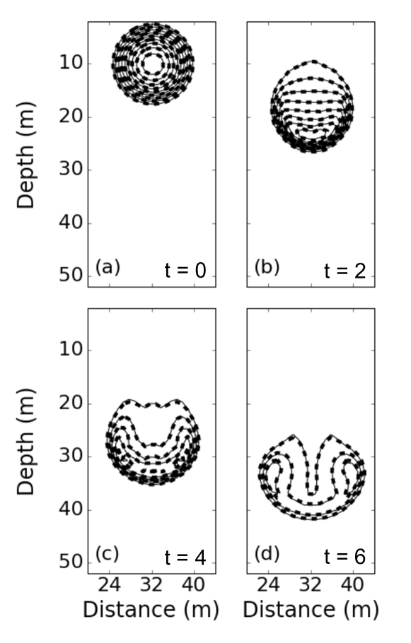
Figure 14: Results from a buoyant bubble test. The thin solid lines are the buoyancy bubble dependent on temperature only. The thicker dashed lines are results from the buoyant bubble dependent on salinity alone. The respective perturbations in temperature and salinity have equivalent buoyancy perturbations. Labels in panels (a) - (d) are the time in minutes from the start of the simulation.

The buoyancy changes and the corresponding salinity flux implementation are validated in a free convection simulation due to surface evaporation (CEW; Table 2). The agreement in the location of the buoyancy flux minimum diagnosed from the LES model and the analytic solution (see Appendix E) is quite good (not shown). Given these results, we have confidence in the comparison of salinity from CVMix to LES for the simulations described in Tables 2 - 3 and Sections 4 - 6.

Appendix D Form of solar radiation

In the LES and single column tests, the shortwave radiation is assumed to obey a Jerlov type IB extinction profile (Paulson and Simpson, 1977). The time variation of incident shortwave radiation ($\mbox{W}~{}\mbox{}~{}\mbox{m}^{-2}$; $F_{sw}(t)$) is given as

$$F_{\mbox{\tiny sw}}(t)=Q_{\mbox{\tiny sw}}^{\mbox{\tiny max}}\max\left\{\cos\left[2\pi\left(\frac{t}{T}-\frac{1}{2}\right)\right],0\right\}$$ (51)

where $t$ is the time in seconds and $T=86400$ are the number of seconds in one day. The peak incoming shortwave radiation ($Q_{\mbox{\tiny sw}}^{\mbox{\tiny max}}$) is determined by forcing a balance between the daily integrated buoyancy gain and the daily integrated buoyancy loss ($\mbox{m}^{2}~{}\mbox{s}^{-3}$), i.e.,

$$\int_{0}^{T}\frac{g\,\alpha_{\theta}}{\rho\,c_{p}}\,F_{\mbox{\tiny sw}}(t)\,\mathrm{d}t\;=\;-\int_{0}^{T}\overline{w^{\prime}\,b^{\prime}}_{\mbox{\tiny sfc}}\,\mathrm{d}t$$ (52)

where this equation has been multiplied by the gravitational acceleration, $g$, and the thermal expansion coefficient, $\alpha_{\theta}$ (equation (23a)) and divided by the reference density and $c_{p}\equiv 4200~{}\mbox{J}~{}\mbox{kg}^{-1}~{}^{\circ}\mbox{C}^{-1}$ to ensure consistent units. Upon integration, and using equation (51), the maximum surface shortwave radiation is given as

$$Q_{\mbox{\tiny sw}}^{\mbox{\tiny max}}=-\pi\left(\frac{\rho\,c_{p}\overline{w^{\prime}b^{\prime}}_{\mbox{\tiny sfc}}}{g\,\alpha_{\theta}}\right).$$ (53)

The units of equation (53) are ($\mbox{m}~{}\mbox{}^{\circ}\mbox{C}~{}\mbox{s}^{-1}$) given the division by $g\,\alpha_{\theta}$.

Appendix E Analytic boundary layer solution

The derivation in this appendix follows previous work closely (Turner, 1973; Haine and Marshall, 1998), but here we do not assume the entrainment of fluid into the boundary layer is negligible. Assuming that entrainment into the boundary layer is negligible is equivalent to assuming that $h=h_{e}=h_{m}$ in KPP (Figure 2). In this derivation we relax this assumption slightly by assuming the buoyancy jump between the boundary layer and interior is large but not a discontinuity (i.e., $h\approx h_{e}\approx h_{m}$).

We begin by assuming that a model is forced with a horizontally uniform, constant in time, buoyancy flux, which simplifies the buoyancy equation to

$$\frac{\partial b}{\partial t}=-\frac{\partial\overline{w^{\prime}b^{\prime}}}{\partial z}.$$ (54)

Next, equation (54) is integrated from the surface $(z=0)$ to a depth $-H$ below the boundary layer ($h$) that does not change in time, i.e.,

$$\int_{-H}^{0}\frac{\partial b}{\partial t}\;dz=-\int_{-H}^{0}\frac{\partial\overline{w^{\prime}b^{\prime}}}{\partial z}\;dz.$$ (55)

Assuming $\overline{w^{\prime}b^{\prime}}$ is small at a depth $H$ below the boundary layer, equation (55) can be written as

$$\frac{\partial}{\partial t}\int_{-H}^{0}b(z)\;dz=-\overline{w^{\prime}b^{\prime}}_{z=0}.$$ (56)

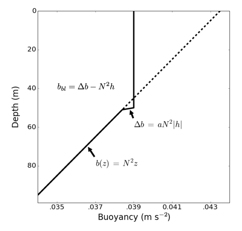
Figure 15: Schematic illustrating the analytic buoyancy solution. The dashed line is the initial stratification, and the solid line is the profile after some time (t). The buoyancy change across the entrainment layer is assumed to be a small fraction of the interior stratification ($a<<1$). Thus this case does not assume a jump discontinuity between the well-mixed layer and the interior ocean. Yet, given that the buoyancy change is large, $h_{e}\approx h$ (Figure 2).

We now need to assume a buoyancy profile for the upper ocean. The assumed form is shown in Figure 15. The buoyancy is uniform in the boundary layer, the stratification is constant below the boundary layer, and there is a sharp (but not discontinuous) buoyancy change between the well-mixed layer and the interior ocean, (similar to VanZanten et al., 1999). The strength of the buoyancy jump is assumed to be equal to the deep ocean buoyancy at the boundary layer base (i.e., $N^{2}|h|$) multiplied by a small constant ($a$), which is assumed to be less than one. With this assumption, the boundary layer buoyancy is

$$b(h)=\Delta b-N^{2}|h|=(a-1)N^{2}|h|.$$ (57)

Using equation (57), (56) can be written as

$$\frac{\partial}{\partial t}\left[\int_{-H}^{-h(t)}N^{2}zdz+\int_{-h(t)}^{0}(a-1)N^{2}|h|dz\right]=\overline{w^{\prime}b^{\prime}}_{\mbox{\tiny sfc}}.$$ (58)

Equation (58) can be easily integrated to find

$$(1-2a)N^{2}\frac{\partial}{\partial t}\left[\frac{h^{2}}{2}\right]=\overline{w^{\prime}b^{\prime}}_{\mbox{\tiny sfc}}.$$ (59)

The constant $a$ is determined by using the formula for the boundary layer heat flux from Lilly (1968) and the empirical rule of convection

$$\frac{\overline{w^{\prime}b^{\prime}}(h_{e})}{\overline{w^{\prime}b^{\prime}}_{sfc}}\approx 0.2.$$ (60)

Since the buoyancy change is sharp, $h_{e}\approx h$, and $\overline{w^{\prime}b^{\prime}}(h)\approx\overline{w^{\prime}b^{\prime}}(h_{e})$. Equating the empirical rule of convection and the boundary layer heat flux formula from Lilly (1968) yields

$$\overline{w^{\prime}b^{\prime}}(h)=\Delta b\,\frac{\partial h}{\partial t}=0.2\,\overline{w^{\prime}b^{\prime}}_{\mbox{\tiny sfc}}.$$ (61)

Using the assumed form of the entrainment layer buoyancy change, equation (61) becomes

$$aN^{2}|h|\frac{\partial h}{\partial t}=aN^{2}\frac{\partial}{\partial t}\left(\frac{h^{2}}{2}\right)=0.2\,\overline{w^{\prime}b^{\prime}}_{\mbox{\tiny sfc}}.$$ (62)

Dividing equation (62) by equation (59) gives

$$\frac{a}{1-2a}=0.2.$$ (63)

Equation (63) gives $a\approx 0.143$. Inserting this result into equation (59), the final expression for boundary layer depth is

$$h(t)=\left(\frac{2.8\;\overline{w^{\prime}b^{\prime}}_{sfc}\;t}{N^{2}}\right)^{1/2}.$$ (64)

References

- Abarbanel et al. (1984) Abarbanel, H. D., D. D. Holm, J. E. Marsden, and T. Ratiu (1984), Richardson number criterion for the nonlinear stability of three-dimensional stratified flow, Phys. Rev. Lett., 52(26), 2352.
- Adcroft and Hallberg (2006) Adcroft, A., and R. Hallberg (2006), On methods for solving the oceanic equations of motion in generalized vertical coordinates, Ocean Model., 11(1), 224–233.
- Arakawa and Lamb (1981) Arakawa, A., and V. R. Lamb (1981), A potential enstrophy and energy conserving scheme for the shallow water equations, Monthly Weather Review, 109(1), 18–36.
- Ayotte et al. (1996) Ayotte, K. W., P. P. Sullivan, A. Andren, S. C. Doney, A. A. M. Holtslag, W. G. Large, J. C. McWilliams, C.-H. Moeng, M. J. Otte, J. J. Tribbia, and J. C. Wyngaard (1996), An evaluation of neutral and convective planetary boundary-layer parameterizations relative to large eddy simulations, Bound.-Lay. Meteorol., 79, 131–175.
- Bachman et al. (2017) Bachman, S., B. Fox-Kemper, J. Taylor, and L. Thomas (2017), Parameterization of frontal symmetric instabilities. I: Theory for resolved fronts, Ocean Model., 109, 72–95.
- Barad and Fringer (2010) Barad, M. F., and O. B. Fringer (2010), Simulations of shear instabilities in interfacial gravity waves, J. Fluid Mech., 644, 61–95.
- Boccaletti et al. (2007) Boccaletti, G., R. Ferrari, and B. Fox-Kemper (2007), Mixed layer instabilities and restratification, Journal of Physical Oceanography, 35, 1263–1278.
- Brown and Grant (1997) Brown, A., and A. Grant (1997), Non-local mixing of momentum in the convective boundary layer, Boundary-Layer Meteorology, 84(1), 1–22.
- Brown (1996) Brown, A. R. (1996), Evaluation of parametrization schemes for the convective boundary layer using large-eddy simulation results, Bound.-Lay. Meteorol., 81(2), 167–200.
- Burchard and Bolding (2001) Burchard, H., and K. Bolding (2001), Comparative analysis of four second-moment turbulence closure models for the oceanic mixed layer, Journal of Physical Oceanography, 31(8), 1943–1968.
- Canuto et al. (2001) Canuto, V. M., A. Howard, Y. Cheng, and M. S. Dubovikov (2001), Ocean turbulence. Part I: One-point closure model—momentum and heat vertical diffusivities, J. Phys. Oceanogr., 31(6), 1413–1426.
- Canuto et al. (2007) Canuto, V. M., Y. Cheng, and A. M. Howard (2007), Non-local ocean mixing model and a new plume model for deep convection, Ocean Model., 16(1-2), 28–46.
- Danabasoglu et al. (2006) Danabasoglu, G., W. G. Large, J. J. Tribbia, P. R. Gent, B. P. Briegleb, and J. C. McWilliams (2006), Diurnal coupling in the tropical oceans of CCSM3, J. Climate, 19(11), 2347–2365.
- Deardorff (1966) Deardorff, J. W. (1966), The counter-gradient Heat Flux in the Lower atmosphere and laboratory, J. Atmos. Sci., pp. 503–506.
- Deardorff (1972) Deardorff, J. W. (1972), Theoretical expression for countergradient vertical heat-flux, J. Geophys. Res., 77(30), 5900–5904.
- Deardorff (1980) Deardorff, J. W. (1980), Stratocumulus-capped mixed layers derived from a three-dimensional model, Bound.-Lay. Meteorol., 18(4), 495–527.
- Donaldson (1972) Donaldson, C. D. (1972), Calculation of turbulent shear flows for atmospheric and vortex motions, AIAA, 10(1), 4–12.
- Ertel (1942) Ertel, H. (1942), The vertical turbulent heat flux in the atmosphere, Meteorol. Zeitschr, 59, 250–253.
- Fox-Kemper et al. (2008) Fox-Kemper, B., R. Ferrari, and R. Hallberg (2008), Parameterization of mixed layer eddies. I: Theory and diagnosis, Journal of Physical Oceanography, 38, 1145–1165.
- Frech and Mahrt (1995) Frech, M., and L. Mahrt (1995), A two-scale mixing formulation for the atmospheric boundary layer, Boundary-Layer Meteorology, 73(1-2), 91–104.
- Gaspar (1988) Gaspar, P. (1988), Modeling the seasonal cycle of the upper ocean, J. Phys. Oceanogr., 18(2), 161–180.
- Griffies et al. (2015) Griffies, S. M., M. Levy, A. J. Adcroft, G. Danabasoglu, R. W. Hallberg, D. Jacobsen, W. Large, and T. D. Ringler (2015), Theory and numerics of the Community Ocean Vertical Mixing (CVMix) Project, Tech. rep.
- Haine and Marshall (1998) Haine, T. W., and J. Marshall (1998), Gravitational, symmetric, and baroclinic instability of the ocean mixed layer, J. Phys. Oceanogr., 28(4), 634–658.
- Hallberg (2003) Hallberg, R. W. (2003), The suitability of large-scale ocean models for adapting parameterizations of boundary mixing and a description of a refined bulk mixed layer model, in Near-Boundary Processes and Their Parameterization, edited by P. Müller and C. Garrett, Proceedings of the 13th ’Aha Huliko’a Hawaiian Winter Workshop, pp. 187–203, University of Hawaii at Manoa.
- Harcourt (2015) Harcourt, R. R. (2015), An improved second-moment closure model of Langmuir turbulence, J. Phys. Oceanogr., 45(1), 84–103.
- Holtslag and Moeng (1991) Holtslag, A. A. M., and C.-H. Moeng (1991), Eddy diffusivity and countergradient transport in the convective atmospheric boundary layer, J. Atmos. Sci., 48(14), 1690–1698.
- Johnson et al. (2002) Johnson, G. C., B. M. Sloyan, W. S. Kessler, and K. E. McTaggart (2002), Direct measurements of upper ocean currents and water properties across the tropical pacific during the 1990s, Progress in Oceanography, 52(1), 31–61.
- Kantha and Clayson (1994) Kantha, L. H., and C. A. Clayson (1994), An improved mixed layer model for geophysical applications, J. Geophys. Res., 99(C12), 25,235–25,266.
- Kato and Phillips (1969) Kato, H., and O. Phillips (1969), On the penetration of a turbulent layer into stratified fluid, Journal of Fluid Mechanics, 37(4), 643–655.
- Kraus and Turner (1967) Kraus, E. B., and J. S. Turner (1967), A one-dimensional model of the seasonal thermocline II. The general theory and its consequences, Tellus, 19(1), 98–106.
- Lappen and Randall (2001) Lappen, C.-L., and D. A. Randall (2001), Toward a unified parameterization of the boundary layer and moist convection. part i: A new type of mass-flux model, Journal of the atmospheric sciences, 58(15), 2021–2036.
- Large and Gent (1999) Large, W. G., and P. R. Gent (1999), Validation of vertical mixing in an equatorial ocean model using large eddy simulations and observations, J. Phys. Oceanogr., 29, 449–464.
- Large et al. (1994) Large, W. G., J. C. McWilliams, and S. C. Doney (1994), Oceanic vertical mixing: A review and a model with a nonlocal boundary layer parameterization, Rev. Geophys., 32(4), 363–403.
- Lemarié et al. (2012) Lemarié, F., J. Kurian, A. F. Shchepetkin, M. J. Molemaker, F. Colas, and J. C. McWilliams (2012), Are there inescapable issues prohibiting the use of terrain-following coordinates in climate models?, Ocean Modelling, 42, 57–79.
- Li et al. (2015) Li, Q., A. Webb, B. Fox-Kemper, A. Craig, G. Danabasoglu, W. G. Large, and M. Vertenstein (2015), Langmuir mixing effects on global climate: WAVEWATCH III in CESM, Ocean Model., pp. 1–16.
- Li et al. (2001) Li, X., J. McWilliams, and L.-L. Fu (2001), A Comparison of two vertical-mixing schemes in a Pacific Ocean General Circulation Model, Mon. Weather Rev., 14, 1377–1398.
- Lilly (1968) Lilly, D. K. (1968), Models of cloud-topped mixed layers under a strong inversion, Q. J. Roy. Met. Soc., 94(401), 292–309.
- Mailhot and Benoit (1982) Mailhot, J., and R. Benoit (1982), A finite-element model of the atmospheric boundary layer suitable for use with numerical weather prediction models., J. Atmos. Sci., 39, 2249–2266.
- McGrath-Spangler et al. (2015) McGrath-Spangler, E. L., A. Molod, L. E. Ott, and S. Pawson (2015), Impact of planetary boundary layer turbulence on model climate and tracer transport, Atmos. Chem. Phys., 15(13), 7269–7286.
- McWilliams and Sullivan (2000) McWilliams, J. C., and P. P. Sullivan (2000), Vertical mixing by Langmuir Circulations, Spill Sci. Technol. Bull., 6(3-4), 225–237.
- McWilliams et al. (1997) McWilliams, J. C., P. P. Sullivan, and C.-H. Moeng (1997), Langmuir turbulence in the ocean, J. Fluid Mech., 334, 1–30.
- Mellor and Yamada (1982) Mellor, G. L., and T. Yamada (1982), Development of a turbulence closure model for geophysical fluid problems, Rev. Geophys., 20(4), 851–875.
- Miles (1961) Miles, J. W. (1961), On the stability of heterogeneous shear flows, J. Fluid Mech., 10(04), 496–508.
- Mironov (2001) Mironov, D. V. (2001), Pressure-potential-temperature covariance in convection with rotation, Quarterly Journal of the Royal Meteorological Society, 127(571), 89–110.
- Moeng and Sullivan (1994) Moeng, C.-H., and P. P. Sullivan (1994), A comparison of shear- and buoyancy-driven planetary boundary layer flows, J. Atmos. Sci., 51(7), 999–1022.
- Moeng and Wyngaard (1984) Moeng, C.-H., and J. C. Wyngaard (1984), Statistics of conservative scalars in the convective boundary layer, J. Atmos. Sci., 41(21), 3161–3169.
- Mukherjee and Tandon (2016) Mukherjee, S., and A. Tandon (2016), Comparison of the simulated upper-ocean vertical structure using 1-dimensional mixed-layer models, Ocean Science Discussions, 2016, 1–22, 10.5194/os-2016-45.
- Niiler and Kraus (1977) Niiler, P. P., and E. B. Kraus (1977), One-dimensional models of the upper ocean, Oregon State University, School of Oceanography.
- Noh et al. (2003) Noh, Y., W. G. Cheon, S. Y. Hong, and S. Raasch (2003), Improvement of the K-profile model for the planetary boundary layer based on large eddy simulation data, Bound.-Lay. Meteorol., 107(2), 401–427.
- Noh et al. (2016) Noh, Y., H. Ok, E. Lee, T. Toyoda, and N. Hirose (2016), Parameterization of Langmuir circulation in the ocean mixed layer model using LES and its application to the OGCM, J. Phys. Oceanogr., 46(1), 57–78.
- O’Brien (1970) O’Brien, J. J. (1970), A note on the vertical structure of the eddy exchange coefficient in the Planetary Boundary Layer, J. Atmos. Sci., 27, 1213–1215.
- Paulson and Simpson (1977) Paulson, C. A., and J. J. Simpson (1977), Irradiance measurements in the upper ocean, J. Phys. Oceanogr., 7(6), 952–956.
- Price et al. (1986) Price, J. F., R. A. Weller, and R. Pinkel (1986), Diurnal cycling: Observations and models of the upper ocean response to diurnal heating, cooling, and wind mixing, J. Geophys. Res., 91(C7), 8411–8427.
- Reffray et al. (2015) Reffray, G., R. Bourdalle-Badie, and C. Calone (2015), Modelling turbulent vertical mixing sensitivity using a 1-D version of NEMO, Geoscientific Model Development, 8(1), 69–86.
- Reichl et al. (2016) Reichl, B. G., D. Wang, T. Hara, I. Ginis, and T. Kukulka (2016), Langmuir turbulence parameterization in tropical cyclone conditions, J. Phys. Oceanogr., 46(3), 863–886.
- Ringler et al. (2013) Ringler, T., M. Petersen, R. L. Higdon, D. Jacobsen, P. W. Jones, and M. Maltrud (2013), A multi-resolution approach to global ocean modeling, Ocean Model., 69, 211–232.
- Seidel et al. (2010) Seidel, D. J., C. O. Ao, and K. Li (2010), Estimating climatological planetary boundary layer heights from radiosonde observations: Comparison of methods and uncertainty analysis, J. Geophys. Res., 115.
- Smith et al. (2010) Smith, R., P. Jones, B. Briegleb, F. Bryan, G. Danabasoglu, J. Dennis, J. Dukowicz, et al. (2010), The Parallel Ocean Program (POP) reference manual ocean component of the Community Climate System Model (CCSM) and Community Earth System Model (CESM).
- Smyth et al. (2002) Smyth, W. D., E. D. Skyllingstad, G. B. Crawford, and H. Wijesekera (2002), Nonlocal fluxes and Stokes drift effects in the K-profile parameterization, Ocean Dynam., 52(3), 104–115.
- Soares et al. (2004) Soares, P., P. Miranda, A. Siebesma, and J. Teixeira (2004), An eddy-diffusivity/mass-flux parametrization for dry and shallow cumulus convection, Quarterly Journal of the Royal Meteorological Society, 130(604), 3365–3383.
- Stull (1993) Stull, R. B. (1993), Review of non-local mixing in turbulent atmospheres: Transilient turbulence theory, Boundary-Layer Meteorology, 62(1), 21–96.
- Sullivan et al. (2007) Sullivan, P. P., J. C. McWilliams, and W. K. Melville (2007), Surface gravity wave effects in the oceanic boundary layer: large-eddy simulation with vortex force and stochastic breakers, J. Fluid Mech., 593, 405–452.
- Troen and Mahrt (1986) Troen, I. B., and L. Mahrt (1986), A simple model of the atmospheric boundary layer; sensitivity to surface evaporation, Bound.-Lay. Meteorol., 37(1-2), 129–148.
- Troy and Koseff (2005) Troy, C. D., and J. R. Koseff (2005), The instability and breaking of long internal waves, J. Fluid Mech., 543, 107–136.
- Turner (1973) Turner, J. (1973), Bouyancy effects in fluids, Cambridge University Press, 367p.
- Umlauf and Burchard (2005) Umlauf, L., and H. Burchard (2005), Second-order turbulence closure models for geophysical boundary layers. A review of recent work, Cont. Shelf Res., 25(7-8), 795–827.
- Van Roekel et al. (2012) Van Roekel, L., B. Fox-Kemper, P. Sullivan, P. Hamlington, and S. Haney (2012), The form and orientation of langmuir cells for misaligned winds and waves, Journal of Geophysical Research: Oceans, 117(C5).
- Van Roekel and Maloney (2012) Van Roekel, L. P., and E. D. Maloney (2012), Mixed layer modeling in the East Pacific warm pool during 2002, Climate Dynam., 38(11-12), 2559–2573.
- VanZanten et al. (1999) VanZanten, M. C., P. G. Duynkerke, and J. W. M. Cuijpers (1999), Entrainment parameterization in convective boundary layers, J. Atmos. Sci., 56(6), 813–828.
- Vogelzang and Holtslag (1996) Vogelzang, D. H. P., and A. A. M. Holtslag (1996), Evaluation and model impacts of alternative boundary-layer height formulations, Bound.-Lay. Meteorol., 81(3), 245–269.
- Wang et al. (1998) Wang, D., J. C. McWilliams, and W. G. Large (1998), Large-eddy simulation of the diurnal cycle of deep equatorial turbulence, J. Phys. Oceanogr., 28(1), 129–148.
- Zedler et al. (2002) Zedler, S. E., T. D. Dickey, S. C. Doney, J. F. Price, X. Yu, and G. L. Mellor (2002), Analyses and simulations of the upper ocean’s response to Hurricane Felix at the Bermuda testbed Mooring site: 13-23 August 1995, J. Geophys. Res., 107(C12), 25–1–25–29.