An Algorithm to Compress Line-transition Data for Radiative-transfer Calculations
Abstract
Molecular line-transition lists are an essential ingredient for radiative-transfer calculations. With recent databases now surpassing the billion-lines mark, handling them has become computationally prohibitive, due to both the required processing power and memory. Here I present a temperature-dependent algorithm to separate strong from weak line transitions, reformatting the large majority of the weaker lines into a cross-section data file, and retaining the detailed line-by-line information of the fewer strong lines. For any given molecule over the 0.3–30 m range, this algorithm reduces the number of lines to a few million, enabling faster radiative-transfer computations without a significant loss of information. The final compression rate depends on how densely populated is the spectrum. I validate this algorithm by comparing Exomol’s HCN extinction-coefficient spectra between the complete (65 million line transitions) and compressed (7.7 million) line lists. Over the 0.6–33 m range, the average difference between extinction-coefficient values is less than 1%. A Python/C implementation of this algorithm is open-source and available at https://github.com/pcubillos/repack. So far, this code handles the Exomol and HITRAN line-transition format.
1 INTRODUCTION
The study of exoplanet atmospheres and their spectra critically depends on the available laboratory and theoretical data of gaseous species (Fortney et al., 2016). The discovery of highly irradiated sub-stellar atmospheres has motivated the compilation of molecular line-transition lists at temperatures far above those of the Earth atmosphere (Rothman et al., 2010; Tennyson et al., 2016). However, these newest databases are starting to grow into the billions of line transitions (e.g., Rothman et al., 2010; Yurchenko et al., 2011; Yurchenko & Tennyson, 2014).
To date, medium- to low-resolution multi-wavelength observations of exoplanets cover a broad wavelength range (0.3 to 30 m), requiring the use of the line-transition data nearly in their entirety. With the arrival of future facilities, like the James Webb Space Telescope (JWST), this picture will remain. Such large line-transition data files render radiative-transfer calculations computationally prohibitive, both in terms of the necessary memory and processing power.
To keep the molecular line lists manageable, authors commonly set a fixed opacity cutoff, discarding all lines weaker than a certain threshold (e.g., Sharp & Burrows, 2007). However, this approach is at best below optimal, as one could remove entire absorption bands at certain wavelengths, or retain a large number of line-transitions that do not significantly contribute to the opacity.
Inspired by the idea of Hargreaves et al. (2015) of separating line-by-line and continuum line-transition information, I devised an algorithm to reduce the amount of line-transition data required for radiative-transfer calculations, with minimal loss of information. Using this approach, one retains the full information only of the stronger lines that dominate the absorption spectrum, and compresses the combined information of the many-more weak lines into a cross-section data file, as a function of wavenumber and temperature. Since, the interpretation of mid- and low-resolution observations relies more on the total opacity contribution rather than the individual line transitions, this algorithm allows for a significant performance improvement of radiative-transfer calculations.
2 METHODS
The integrated absorption intensity (or opacity or extinction coefficient) of a line transition (in cm-1) can be expressed as
| (1) |
where , , and are the weighted oscillator strength, central wavenumber, and lower-state energy level of the line transition , respectively; and are the partition function and number density of the isotope , respectively; is the temperature; and are the electron’s charge and mass, respectively; is the speed of light, is Planck’s constant; and is the Boltzmann’s constant.
For any given molecule, the number density of an isotope can be written as , where is the molecule number density and is the isotopic abundance fraction (which can be assumed to be at Earth values). Then, by knowing the set of isotopic fractions for a given molecule, we can express the line intensities per unit of the molecule’s number density (in cm2molec-1) as .
To compute the extinction-coefficient spectrum, one needs to broaden each line according to the Voigt profile function (the convolution of a Doppler and a Lorentz profile), and then summing the contribution from all lines. Thus, to identify the dominant lines, one has to consider the dilution of the line intensity by the Voigt broadening.
In practice, for a given molecule, the Voigt broadening profile varies weakly over neighboring lines. Since the Doppler broadening is simpler to compute than the Lorentz profile, I approximate the Voigt broadening by the Doppler broadening profile:
| (2) |
with line width
| (3) |
where is the mass of the isotope.
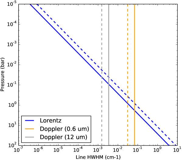
Figure 1 shows the typical values for the Doppler and Lorentz half-width at half-maximum (HWHM) for exoplanet atmospheres. The Doppler broadening dominates the line profile above 0.3 bar, across temperature ranges of 500 to 2500 K and wavelengths of 0.6 to 12 m. In this pressure range, the line-transition widths range between cm-1 and cm-1, depending on the wavelength and atmospheric parameters. Cubillos et al. (2017b, submitted) studied the atmospheric pressures probed by transmission and emission spectroscopy of gaseous exoplanets, for a wide range of planetary properties. They found that the typical optical-to-infrared transmission observations probe pressures between 1 and bar, whereas day-side emission observations probe between 10 and bar. Therefore, most of the observable atmosphere is under the Doppler broadening regime. If one approximates the lineshape by the Doppler profile, Eq. (2) tells then that the maximum intensity of a line is approximately (hereafter, called diluted line intensity). In Section 3.1 we show that this is an acceptable assumption, even when there is significant Lorentz broadening, for medium or low-resolution observations.
2.1 Line-flagging Algorithm
To efficiently identify dominant from weak lines, one can start by selecting the strongest line in a given wavelength range, say line transition , and compute its Doppler profile . Then, one flags out the surrounding lines whose diluted intensity () is smaller than the profile of line , with a threshold tolerance , i.e.:
| (4) |
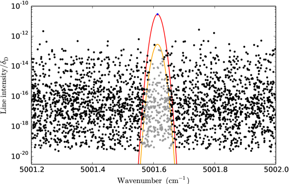
Since the line intensity decays exponentially as one moves away from its center, the flagged (weak) lines do not significantly contribute to the extinction coefficient. This effectively avoids the need to broaden most of the lines in a database. Line intensities span several orders of magnitude, and thus, only the few strongest lines at any given wavelength dominate the absorption spectrum (Figure 2). The algorithm then proceeds with the next un-flagged strongest line transition, and so on.
Now, different lines can dominate the spectrum depending on the atmospheric temperature (see Eq. (1)). To account for this, one repeats the flagging process at the two extreme temperatures to consider (a user choice, for example, 300 and 3000 K is appropriate for sub-stellar objects).
After one identifies strong and weak lines, one preserves the full line-by-line information only for the strong lines (for radiative transfer, the , , , and the isotope ID suffice). The information from the large majority of weak lines can be compressed into a continuum extinction coefficient table as function of wavelength and temperature. To avoid broadening each line, one simply add the line intensity to the nearest tabulated wavenumber point, diluting the line according to the wavenumber sampling rate (following Sharp & Burrows, 2007).
3 Open-source Implementation
Along with this article, I provide an open-source version of this algorithm (under the MIT license), available at https://github.com/pcubillos/repack. This is a Python package (accelerated with C subroutines) compatible with Python2 and Python3, running on both Linux and OSX. This package handles the Exomol and HITRAN input line-transition formats. The routine’s performance, varies with the size of the initial database, the number of evaluated profiles (which depends on ), and how densely packed are the line transitions. For an Intel Core i7-4790 3.60 GHz CPU, the routine runs the Exomol HCN (65 million lines, Harris et al., 2006, 2008; Barber et al., 2014), NH3 (1 billion, Yurchenko et al., 2011), and CH4 (10 billion, Yurchenko & Tennyson, 2014) databases in 10 minutes, 7 hours, and 5 days, respectively. The performance scales somewhat faster than linear with the number of line transitions. Certainly, the gain of working with the compressed line lists more than compensates for the time spent running this routine (a one-time run) for the largest data bases. Ultimately the line-by-line compression rate will depend on how compact or saturated is a line list. For example, with a threshold tolerance of 0.01, this algorithm compresses the Exomol HCN database by 90% in the 0.6–33 m range. The algorithm compresses the denser Exomol NH3 line list (1 billion) by 95%.
3.1 Validation
To validate the compression algorithm, I compare the extinction-coefficient spectra produced from the compressed and the complete line-by-line database for HCN from Exomol. This data base comprises 65 million lines over the 0.6–33.0 m range. Adopting a threshold tolerance of , and temperature values between 500 and 3000 K, the algorithm retains 7.7 million lines.
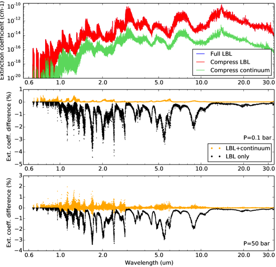
To compute the HCN’s extinction-coefficient spectrum, I use the Python Radiative-transfer in a Bayesian framework package (Pyrat Bay111http://pcubillos.github.io/pyratbay, Cubillos et al., 2017a, in prep.). Pyrat Bay is based on the Bayesian Atmospheric Radiative Transfer package (Blecic, 2016; Cubillos, 2016). Figure 3 (top panel) shows the resulting spectra for a typical Jupiter-composition planet, at an atmospheric temperature of 1540 K and pressure of 0.1 bar. Figure 3 (middle panel) shows the difference in extinction coefficient between the full line-list and the compressed dataset. The spectra for this panel simulate an instrumental resolving power of 1 cm-1 (approximately the highest resolution that the JWST instruments will achieve). The LBL component alone reproduces the full line-list extinction coefficient down to 1% on average, and down to a few percent in the worst case. When, considering both the LBL and continuum components, the compressed dataset reproduces the full line-list spectrum well under 1%.
At higher pressures, where the Lorentz profile dominates the line
broadening, the compressed dataset still reproduces well the full
line-list spectrum (Fig. 3, bottom panel). Some
over-estimated values arise because the compressed continuum opacity
does not consider the Lorentz broadening. However, the differences
are still on the order of a few percent.
The mismatch varies with the given instrumental resolution,
with a coarser resolution producing smaller differences.
In summary, I presented an efficient compression algorithm that identifies the line transitions that dominate a spectrum. This algorithm is aimed to serve radiative-transfer modeling of medium to low spectral resolution data over broad wavelength ranges, like that of the JWST.
References
- AAS Journals Team & Hendrickson (2016) AAS Journals Team, & Hendrickson, A. 2016, AASJournals/AASTeX60: Version 6.1
- Barber et al. (2014) Barber, R. J., Strange, J. K., Hill, C., Polyansky, O. L., Mellau, G. C., Yurchenko, S. N., & Tennyson, J. 2014, MNRAS, 437, 1828, ADS, 1311.1328
- Blecic (2016) Blecic, J. 2016, ArXiv e-prints, ADS, 1604.02692
- Cubillos et al. (2017a) Cubillos, P., Blecic, J., & Harrington, J. 2017a, in prep.
- Cubillos et al. (2017b) Cubillos, P., Kubyshkina, D., Fossati, L., Mordasini, C., & Lendl, M. 2017b, submitted.
- Cubillos (2016) Cubillos, P. E. 2016, ArXiv e-prints, ADS, 1604.01320
- Fortney et al. (2016) Fortney, J. J. et al. 2016, ArXiv e-prints, ADS, 1602.06305
- Hargreaves et al. (2015) Hargreaves, R. J., Bernath, P. F., Bailey, J., & Dulick, M. 2015, ApJ, 813, 12, ADS, 1510.06982
- Harris et al. (2008) Harris, G. J., Larner, F. C., Tennyson, J., Kaminsky, B. M., Pavlenko, Y. V., & Jones, H. R. A. 2008, MNRAS, 390, 143, ADS, 0807.0717
- Harris et al. (2006) Harris, G. J., Tennyson, J., Kaminsky, B. M., Pavlenko, Y. V., & Jones, H. R. A. 2006, MNRAS, 367, 400, ADS, astro-ph/0512363
- Hunter (2007) Hunter, J. D. 2007, Computing In Science & Engineering, 9, 90
- Jones et al. (2001) Jones, E., Oliphant, T., Peterson, P., et al. 2001, SciPy: Open source scientific tools for Python, [Online; accessed 2017-02-12]
- Rothman et al. (2010) Rothman, L. S. et al. 2010, J. Quant. Spec. Radiat. Transf., 111, 2139, ADS
- Sharp & Burrows (2007) Sharp, C. M., & Burrows, A. 2007, ApJS, 168, 140, ADS, arXiv:astro-ph/0607211
- Tennyson et al. (2016) Tennyson, J. et al. 2016, Journal of Molecular Spectroscopy, 327, 73, ADS, 1603.05890
- van der Walt et al. (2011) van der Walt, S., Colbert, S. C., & Varoquaux, G. 2011, Computing in Science & Engineering, 13, 22
- Yurchenko et al. (2011) Yurchenko, S. N., Barber, R. J., & Tennyson, J. 2011, MNRAS, 413, 1828, ADS, 1011.1569
- Yurchenko & Tennyson (2014) Yurchenko, S. N., & Tennyson, J. 2014, MNRAS, 440, 1649, ADS, 1401.4852