Diffusive tidal evolution for migrating hot Jupiters

Abstract

I consider a Jovian planet on a highly eccentric orbit around its host star, a situation produced by secular interactions with its planetary or stellar companions. The tidal interactions at every periastron passage exchange energy between the orbit and the planet’s degree-2 fundamental-mode. Starting from zero energy, the f-mode can diffusively grow to large amplitudes if its one-kick energy gain $\geq 10^{-5}$ of the orbital energy. This requires a pericentre distance of $\leq 4$ tidal radii (or $1.6$ Roche radii). If the f-mode has a non-negligible initial energy, diffusive evolution can occur at a lower threshold. The first effect can stall the secular migration as the f-mode can absorb orbital energy and decouple the planet from its secular perturbers, parking all migrating jupiters safely outside the zone of tidal disruption. The second effect leads to rapid orbit circularization as it allows an excited f-mode to continuously absorb orbital energy as the orbit eccentricity decreases. So without any explicit dissipation, other than the fact that the f-mode will damp nonlinearly when its amplitude reaches unity, the planet can be transported from a few AU to $\sim 0.2$ AU in $\sim 10^{4}$ yrs. Such a rapid circularization is equivalent to a dissipation factor $Q\sim 1$, and it explains the observed deficit of super-eccentric Jovian planets. Lastly, the repeated f-mode breaking likely deposit energy and angular momentum in the outer envelope, and avoid thermally ablating the planet. Overall, this work boosts the case for forming hot Jupiters through high-eccentricity secular migration.

1. Introduction

Hot Jupiters, the first-known population of extra-solar planets (Mayor & Queloz, 1995; Marcy et al., 2005), orbit their stars at implausibly close ranges, so close that they are not thought to have formed locally but have been migrated inward, either by dynamical interactions with other large bodies, or by gas in the protoplanetary disks (Lin & Papaloizou, 1986). In the former scenario (going by a number of flavours, e.g., planet scattering, Kozai-Lidov migration, secular chaos… Ford et al., 2001; Wu & Murray, 2003; Nagasawa et al., 2008; Wu & Lithwick, 2011), angular momentum exchanges between a Jovian planet, originally at a few AU, and its neighbours (either stellar or planetary ones) gradually squeeze the planet’s orbit, causing it approach the star with an ever-decreasing minimum distance. Strong tides are raised on the planet whenever it sweeps by its host star. It is hypothesized then that these tidal sloshing can be dissipated into heat by friction inside the planet, leading to orbital decay and circularization. A hot Jupiter is thus born, as the direct result of tidal dissipation.

While neatly accounting for the presence of hot Jupiters and many of their observed properties (e.g., their tight pile-up at a few times the Roche radii, their lack of nearby-companions, the metal-richness of their host stars…), theories of dynamical migration all share three fatal weaknesses – all related to the tidal process. First, friction inside a gaseous planet like Jupiter has been shown to be too weak, by orders of magnitude, to generate the required dissipation (Goldreich & Nicholson, 1977; Wu, 2005). Second, in numerical simulations, the angular momentum exchanges with their secular perturbers oftentimes push these planets too close to their stars, crucifying them in the process. Hydrodynamics simulations found that if a planet comes inward of $2.7r_{t}$, where the tidal radius $r_{t}=(M_{*}/M_{p})^{1/3}R_{p}$, it will be tidally disrupted within a handful of orbits (Guillochon et al., 2011). Numerically, one finds that up to $90\%$ of migrating hot Jupiters can be pushed inward of this distance and go to waste (Petrovich, 2015; Muñoz et al., 2016; Hamers et al., 2017). As a result, the proposed mechanisms fail to account for the observed frequency of hot Jupiters. Third, in order to circularize the orbits, the tides need to deposit inside the planet an amount of energy that is comparable to or larger than the planet’s binding energy. There is no guarantee that any planet can survive this, rather than be thermally ablated.

Reviving previous investigations by Mardling (1995); Kochanek (1992); Ivanov & Papaloizou (2004), I now consider a tidal process for high eccentricity orbits. This process has the potential to resolve all three of the above weaknesses.

At every periastron passage, tidal stretching and compression excite oscillations inside the planet. Orbital energy is converted into fluid motion, or, the orbital degree of freedom and the internal degrees of freedom are coupled. The most important internal mode for this is an $\ell=2$ f-mode. If one ignores the feedback from the mode to the orbit, the orbit remains strictly periodic and the internal mode is only excited to a finite (and typically small) amplitude, much like that of a harmonic oscillator driven under a periodic, non-resonant force (Press & Teukolsky, 1977; Lee & Ostriker, 1986; Lai, 1997; Smeyers et al., 1991). There is no long-term benefit to this interaction. However, when the closest approach is small enough, it is no longer valid to ignore the feedback. The oscillations can acquire a sufficient amount of energy to alter the orbital period significantly. Mardling (1995); Kochanek (1992) are the first to use numerical simulations to show that the mode energy can now undergo random-walk. And Ivanov & Papaloizou (2004) followed up by illuminating the underlying physics. This goes as follows. At every passage, the f-mode receives a kick from the tidal potential. The magnitude of this kick can be considered roughly constant, as long as the peri-centre distance is kept constant. Its phase, however, depends on the phase of the f-mode pulsation at periastron. This in turn depends on the length of an orbit, which is perturbed by the tidal energy exchange. When this phase is sufficiently random between kicks, the mode can be launched into a random walk with its energy growing roughly linearly in time.

In this work, I extend the result of Ivanov & Papaloizou (2004) by obtaining the quantitative criterion for diffusive tidal evolution. This is performed for the case when the f-mode has zero initial energy (Mardling, 1995; Ivanov & Papaloizou, 2004; Vick & Lai, 2017), and for the case when the f-mode has a finite initial energy (§2). I give simple explanations for these criteria (§3) and consider the impacts of these physics on the migration of hot Jupiters (§4).

2. Energy exchange between Orbit and Mode

To consider the coupled evolution of the orbit and the modes, I use the equations of motion first derived by Lai (1997), following that of Press & Teukolsky (1977). An alternative prescription, based on the variational principle, is derived by Gingold & Monaghan (1980). I consider exclusively tides raised on the planet (mass $M_{p}$, radius $R_{p}$) by the star (point mass $M_{*}$), ignoring effects of mode dissipation (justified later).

I consider a core-less model for Jupiter, $R_{p}=1.1R_{J}$, $M_{p}=1M_{J}$. The slight size inflation mimics a young Jupiter on its cooling contraction ($t\sim 1$ Gyrs). Of most relevance is the period of the $\ell=2$ f-mode. Let us scale the results of Gudkova & Zharkov (1999), $P_{0}=8502\,\rm s$ for Jupiter, by $(R_{p}/R_{J})^{2.1}$ (Le Bihan & Burrows, 2013) to obtain $P_{0}=1.04\times 10^{4}\,\rm s$.

I first focus on the one-kick energy, the amount of energy an f-mode would acquire after one periastron passage, if it has zero initial energy. This is demonstrated to affect the behaviour of the f-mode when multiple passages are considered. Lastly, it is shown that the initial energy of an f-mode also affects the dynamics.

2.1. Equations of Motion

Let ${\bf D}$ be the vector from the centre of the planet to the star. Written in spherical coordinates in the co-moving frame of the planet, ${\bf D}=[D(t),{\pi/2},\Phi(t)]$. The star (mass $M_{*}$) exerts a tidal potential $U({\bf r},t)$ for fluid at position ${\bf r}$ inside the planet and excites motion. I decompose the excited motion, expressed in displacement vector, as ${\bf\xi}=\sum_{\alpha}a_{\alpha}(t){\bf\xi}_{\alpha}({\bf r})+c.c.$, where ${\bf\xi}_{\alpha}$ is the eigenvector for eigenmode $\alpha$, $a_{\alpha}$ its complex amplitude, and $\omega_{\alpha}$ its real frequency (dissipation ignored). As the planet is axis-symmetric, the eigenfunctions can be decomposed in the azimuthal direction into periodic functions (i.e., $\cos(m\phi)$). And in the following, we adopt the sign convention of $e^{i\sigma t+im\phi}$, so a positive $m$ indicates a retrograde mode in the inertial frame, while a negative value that of a prograde one. Here $c.c.$ stands for complex conjugate. The eigenfunction is normalized as $\int d^{3}x\rho{\bf\xi}_{\alpha}\cdot{\bf\xi}^{*}_{\alpha}=M_{p}R_{p}^{2}$. As a result, all perturbed quantities have natural dimensions (e.g., $\xi$ has the dimension of length, and $a_{\alpha}$ is dimensionless). The amplitude of the normal mode is excited by the tidal potential as

$${\ddot{a}}_{\alpha} = -\omega_{\alpha}^{2}a_{\alpha}+\sum_{\ell}{{GM_{*}W_{\ell m}Q_{\alpha\ell}}\over{M_{p}R_{p}^{2}D^{\ell+1}}}e^{-im\Phi}$$ (1)

$$= -\omega_{\alpha}^{2}a_{\alpha}+{{GM_{*}}\over{D^{3}}}\times\left({R_{p}}\over{D}\right)^{\ell-2}\,{W_{\ell m}Q^{\prime}_{n\ell}}e^{-im\Phi}\,.$$

Here, I define a dimensionless form of the tidal integral as

$$Q^{\prime}_{n\ell}={{Q_{n\ell}}\over{M_{p}R_{p}^{\ell}}}={1\over{M_{p}}}\,\int\rho r^{2}\,\left({r\over{R_{p}}}\right)^{\ell}\left({{\delta\rho}\over{\rho}}\right)_{n\ell}\,dr\,.$$ (2)

where $\delta\rho$ is the Lagrangian density perturbation and is related to the displacement ${\bf\xi}_{\alpha}$ by the equation of mass conservation. Definitions for the geometry factor $W_{\ell m}$ and the tidal overlap integral $Q_{n\ell}$ are given in Press & Teukolsky (1977). In our case, the overlap is nonzero only between the $\ell$-term of the tidal potential and a mode with degree $\ell$. Moreover, the dimensionless factor $Q^{\prime}_{n\ell}$ does not depend on planet mass or radius, and is of order unity for f-modes of all spherical degree $\ell$. Numerically, I find $Q^{\prime}_{n\ell}\approx 0.5$ for f-modes.

In the mean time, the gravitational moment of the excited mode acts on the orbit. Together with the monopole potential ($-GM_{*}M_{p}/D$), this moves the orbit as

$${\ddot{D}} = D{\dot{\Phi}}^{2}-{{G(M_{*}+M_{p})}\over D^{2}}\times$$

$$\left[1+\sum_{\alpha}{(\ell+1)}\,\left({{R_{p}}\over{D}}\right)^{\ell}\,{W_{\ell m}Q^{\prime}_{n\ell}}(a_{\alpha}e^{im\Phi}+c.c.)\right]$$

$${{d(D^{2}{\dot{\Phi}})}\over{dt}} = {{G(M_{*}+M_{p})}\over D}\times$$ (3)

$$\sum_{\alpha}im\left({{R_{p}}\over{D}}\right)^{\ell}{W_{\ell m}Q^{\prime}_{n\ell}}(a_{\alpha}e^{im\Phi}+c.c.)\,.$$

Physically, eq. (1)-(3) can be thought of as describing the interactions between two coupled harmonic oscillators (the mode and the orbit). When the coupling strength (tidal interaction) is weak, the oscillators exchange energy periodically, with no long term effect; when it is strong, the exchange is ergodic and drives the system toward energy equi-partition between the two oscillators.

The total energy of the system should remain constant at all times,

$$E_{\rm tot} = E_{\rm orb}+E_{\rm mode}+V_{\rm tide}$$ (4)

$$= -{{GM_{*}M_{p}}\over{D}}+{1\over 2}\mu\left[{\dot{D}}^{2}+(D{\dot{\Phi}})^{2}\right]$$

$$+\sum_{\alpha}\left({\dot{a}_{\alpha}}{\dot{a}_{\alpha}}^{*}+\omega_{\alpha}^{2}a_{\alpha}a_{\alpha}^{*}\right)M_{p}R_{p}^{2}$$

$$-\sum_{\alpha}{{GM_{*}M_{p}}\over D}\left({{R_{p}}\over{D}}\right)^{\ell}{W_{\ell m}Q^{\prime}_{n\ell}}\left[a_{\alpha}e^{im\Phi}+c.c.\right]\,.$$

Here, $\mu=M_{*}M_{p}/(M_{*}+M_{p})$ is the reduced mass, and the last term represents the interaction energy between oscillations and stellar gravity. In practice, the conservation of total energy is used to ascertain the accuracy of our numerical procedure.

Numerical integration of this system requires special attention. With the usual Runge-Kutta technique, the energy error grows rapidly and becomes intolerable after just a few orbits. This is caused both by the rapid mode oscillation and by the extremely small time-step required for a highly eccentric orbit. I construct a special integrator that is analogous to the drift-kick-drift symplectic orbit integrator (Wisdom & Holman, 1991) for planetary dynamics. In the drift phase, the eccentric orbit and the oscillation mode are each advanced forward in time analytically, assuming no interaction; and in the kick phase, they are advanced by the amount of mutual interaction integrated over the entire time-step. This strategy avoids some numerical instabilities, but it still requires a very small time-step ($dt\sim 0.001P$) to ensure satisfactory energy conservation.

2.2. One-Kick Energy

An important quantity in this problem is the amount of energy imparted to a mode after one periastron passage, assuming initially zero amplitude. This quantity reflects the strength of tidal interaction and is later used to separate the long-term evolution into two regimes. Here, I compare the analytical expression for this quantity (first derived by Press & Teukolsky, 1977) against results of numerical integration.

The energy gain for mode $\alpha$ is (Press & Teukolsky, 1977, confirmed for our normalization and complex notation)

$$\Delta E_{\rm kick} = \int dt\int d^{3}x\rho{{\partial{\bf\xi_{\alpha}}}\over{\partial t}}\cdot\nabla U$$ (5)

$$= 4\pi^{2}M_{p}R_{p}^{2}\left({{GM_{*}}\over{D_{p}^{3}}}\right)^{2}\left({{R_{p}}\over{D_{p}}}\right)^{2\ell-4}|Q_{n\ell}^{\prime}|^{2}\,|K_{\ell m}(\omega_{\alpha})|^{2}$$

$$= {4}\pi^{2}M_{p}R_{p}^{2}\left({{R_{p}}\over{D_{p}}}\right)^{2\ell-4}|Q_{n\ell}^{\prime}|^{2}\,{{|K_{\ell m}(\omega_{\alpha})|^{2}}\over{T_{\rm peri}^{4}}}\,,$$

where the periastron distance $D_{p}=a(1-e)$, and $T_{\rm peri}$ is the timescale of periastron passage,

$$T_{\rm peri}\equiv\sqrt{{{D_{p}^{3}}\over{GM_{*}}}}\approx 1.41\times 10^{4}{\rm s}\,\left({{D_{p}}\over{0.02{\rm AU}}}\right)^{3/2}\left({{M_{*}}\over{M_{\odot}}}\right)^{-1/2}\,.$$ (6)

The orbit integral $K_{\ell m}$,

$$K_{\ell m}(\omega)\equiv{{W_{\ell m}}\over{2\pi}}\int dt\left({{D_{p}}\over{D(t)}}\right)^{\ell+1}\exp{i\left[\omega t+m\Phi(t)\right]}\,,$$ (7)

quantifies how well the time-varying tidal potential is interacting with the time-varying oscillation over one orbit and has the dimension of time. Contribution to this integral arises mostly when $D(t)\sim D_{p}$, over a duration $T_{\rm peri}$. So if we write $K_{\ell m}=fT_{\rm peri}$, using the dimensionless factor $f$ to account for both the geometry, and more importantly, the cancellation in the integrated tidal forcing arising from the fact that the mode may oscillate multiple cycles during a single periastron passage, we find $f=0.006$ for our $\ell=2$ , $m=-2$ (prograde) f-mode at $D_{p}=0.02$ AU, and some $3000$ times smaller for the retrograde mode, assuming zero spin. So from now on, I will only focus on the $\ell=2,m=-2$ prograde mode and drop the mode subscript $\alpha$ accordingly.

The $f$-factor drops off exponentially for modes with shorter periods. This excludes all but the longest period (i.e., lowest degree) f-mode as being relevant for tidal interaction. It also suggests that, if the $m\neq 0$ f-mode is shifted to a longer period by planet spin, the strength of tidal interaction increases.

For a parabolic orbit, Lai (1997) provided an analytical expression for $K_{2,-2}$ as

$$K_{2,-2}(\omega)={{2z^{3/2}e^{-{2\over 3}z}}\over{\sqrt{15}}}\left(1-{{\sqrt{\pi}}\over{4\sqrt{z}}}\right)\,T_{\rm peri}\,,$$ (8)

where $z=\sqrt{2}\omega T_{\rm peri}$. I compare this expression with integration results using elliptical orbits (Fig. 1). For orbits with large semi-major axis where the parabolic limit is more appropriate, this expression is reproduced. Importantly, the forcing strength depends only on the value of $D_{p}$, not on the actual shape of the orbit ($a$, $e$). This arises because highly eccentric orbits with the same periastron differ little in geometry from the parabolic trajectory. This independence allows the f-mode to continuously absorb energy as the orbit is being circularized ($D_{p}$ remains roughly constant). In the range of $z$ that is of interest to us, one can further simplify the above expression into a power-law,

$$K_{2,-2}\approx 1.79\times 10^{4}z^{-6}\,T_{\rm peri}\,.$$ (9)

In contrast, for orbits that are more circular (smaller $a$), numerical results show that $K_{\ell m}$ generally lies above eq. (8) and exhibits many resonance features. This is because contribution to the orbit integral is no longer strictly limited to from near the periastron. In the limit that the orbit is circular, the entire orbit contributes and $K_{\ell m}$ is dominated by resonances for which the mode period is an integer fraction of the orbital period. In this work, I will focus on the regime where the parabolic expression is valid. There may be interesting dynamics in the resonant regime.

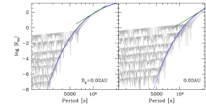
Figure 1.— The logarithm of the orbital integral ($K_{\ell m}$) for the $\ell=2,m=-2$ mode, when the mode period takes on a range of values (horizontal axis, in second). The elliptical orbits take on $D_{p}=0.02$ AU (left panel) and $0.03$ AU (right panel). The seven grey curves in each panel correspond to orbits with a range of semi-major axis, $a=10,5,2,1,0.5,0.2,0.1$ AU (from bottom to top). The numerical results agree with the analytical expression for parabolic orbits (blue lines, eq. 8) at large $a$ (highly eccentric), but deviate from it when $a$ is lower. This is more severe at the right hand panel. The short green lines represent our simple power-law fit (eq. 9).

We are interested in the fractional energy absorption, one that is scaled by the orbital energy. Defining $E_{0}=-E_{\rm tot}-GM_{*}M_{p}/2a_{0}$, we write

$${{\Delta E_{\rm kick}}\over{E_{0}}} \approx 1.3\times 10^{-5}\,\left({a_{0}\over{1{\rm AU}}}\right)\left({{D_{p}}\over{0.02{\rm AU}}}\right)^{-3}\left({{R_{p}}\over{1.1R_{J}}}\right)^{2}\,$$ (10)

$$\times\left[{{Q_{n\ell}^{\prime}}\over{0.5}}\right]^{2}\left[{{K_{\ell m}(\omega)}\over{0.006T_{\rm peri}}}\right]^{2}\,.$$

This quantity drops with increasing $D_{p}$ very steeply – adopting the rough scaling for $K_{\ell m}$ as in eq. (9), $\Delta E_{\rm kick}/E_{0}\propto D_{p}^{-21}$. It also rises with mode period as $P^{6}$. I confirm the analytical expression for the one-kick energy using the numerical integrator.

A few words about the impact of planet spin. At slow rotation, the Coriolis force perturbs the frequency of an $m\neq 0$ mode away from that of the $m=0$ mode as $\omega_{m}=\omega_{0}-m(1-C_{n\ell})\Omega_{s}$, where $\Omega_{s}$ is the spin rate and the rotational splitting integral $C_{n\ell}$ is $C_{n\ell}={1/{M_{p}R_{p}^{2}}}\int r^{2}dr\rho(2\xi_{r}\xi_{h}+\xi_{h}^{2})$. For our $\ell=2$ f-mode, $C_{02}=0.48$, or $\omega_{-2}\approx\omega_{0}+\Omega_{s}$. So, while in a non-rotating planet, the prograde mode couples to the tidal potential much more strongly, in a planet with prograde (relative to the orbit) spin, the prograde mode is shifted to a higher frequency, leading to weaker tidal coupling; in the mean time, its retrograde counterpart now has a lower frequency and can couple more effectively to the tidal potential. This leads to interesting interplay between the planetary spin and mode excitation, a dynamics discussed in detail in Ivanov & Papaloizou (2004).

2.3. Diffusion I: $E_{\rm init}=0$

Evolution after the first passage is studied numerically. With the special integrator, I am able to integrate the dynamics forward for a satisfactory amount of time. In Fig. 2, I present some results of such an integration. The planet is on a highly eccentric orbit of $a=1$AU, $e=0.98$ ($D_{p}=0.02$AU). In this set-up, since the initial orbital energy is of order the binding energy of the planet, the f-mode reaches order unity amplitude (surface radial displacement of order radius) when the mode energy reaches of order $E_{0}$.

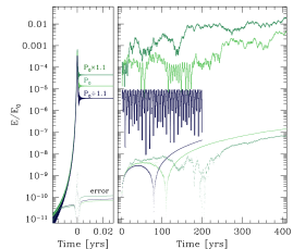
Figure 2.— Tidal excitation over multiple passages for a Jovian planet initially on a $a=1$AU, $D_{p}=0.02$ AU orbit. The solid lines plot the fractional mode energy for the $\ell=2,m=-2$ f-mode when its period is varied from $10\%$ below to $10\%$ above its fiducial value ($P_{0}=1.04\times 10^{4}\,\rm s$), while the dots (lower group) show the fractional energy error in the numerical integrator. The left panel focuses on the first passage (occurring at time zero), and the right panel that over multiple passages. Depending on the value of the one-kick energy, the long-term dynamics bifurcates into two behaviour: lowly excited modes remain oscillating at a few times their one-pass value; while highly excited modes can undergo random-walk in energy. The boundary between the two lies at $\Delta E_{\rm kick}/E_{0}\sim 10^{-5}$.

In each run, I consider a single $\ell=2,m=-2$ f-mode with a slightly different period (ten percent around the fiducial period $P_{0}$) and initially zero energy. As is shown in Fig. 2, after the first passage, the mode acquires a different amount of energy that rises with the f-mode period (eq. 10). And as one continues to integrate the interactions, one sees that there is a bifurcation in mode energy (Mardling, 1995): some exhibit quasi-periodic oscillations in mode energies, with the maxima comparable to or at most a few times larger than the one-kick value; while mode energy in models with longer periods undergo random-walk and rise to larger and larger values over time. As this occurs at the price of the orbital energy, the orbit shrinks. Meanwhile, on account of the small moment of inertia of the planet, the f-modes do not absorb a significant amount of the orbital angular momentum (Ivanov & Papaloizou, 2004). The latter is roughly conserved, with the result that the pericentre distance remains largely constant during the evolution. This in turns allows the f-modes to continue growing unabatedly. The bifurcation between the two behaviour appears to lie where the fractional energy gain $\Delta E_{\rm kick}/|E_{0}|\sim 10^{-5}$. This will be explained in §3.

Our numerical integrator guarantees energy conservation (eq. 4) to better than $10^{-10}$ over every single passage, but as it is not symplectic, energy error does grow with time. The fractional error reaches of order $10^{-7}$ after $\sim 400$ passages. The integration is not be trusted when the energy error becomes comparable to the mode energies, though for models that undergo random-walk, this comes at a much later stage. For these models, our results can be trusted to thousands of orbits and more.

2.4. Diffusion II: $E_{\rm init}>0$

The above bifurcation, for a f-mode with initially zero energy, has been observed by Kochanek (1992); Mardling (1995); Ivanov & Papaloizou (2004). Here, I report on a phenomenon that occurs for f-modes with some initial energies, noted briefly previously by (Mardling, 1995).

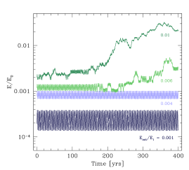
Figure 3.— The time evolution of mode energy (normalized by the orbital energy) for a planet at an orbit of $a=0.5$AU, $D_{p}=0.025$ AU. The expected one-kick energy for this mode ($P=P_{0}=1.04\times 10^{4}\,\rm s$) is $\Delta E_{\rm kick}/E_{0}\sim 8\times 10^{-6}$. This is too weak to have allowed the mode to diffuse, if it starts with zero energy. However, as one endows the mode with an increasing amount of initial energy (values of $E_{\rm init}/E_{1}$ as marked), random-walk sets in again when $E_{\rm init}/E_{1}\geq 0.005$, The rate of diffusion rises with the value of $E_{\rm init}$.

Fig. 3 examines a mode that receives a weak one-kick energy ($\Delta E_{\rm kick}/E_{0}\sim 8\times 10^{-6}$). This should not have undergone diffusion. However, I experiment with endowing the mode with a varying amount of initial energy, quantified by another energy unit, $E_{1}\approx\sqrt{0.1GM_{p}^{2}/R_{p}}=3\times 10^{42}\,\rm erg$. This is the mode energy when its surface radial displacement reaches unity. One finds that whenever $E_{\rm init}/E_{1}\geq 0.005$, corresponding to a surface displacement of $\geq 7\%R_{p}$, diffusion can set in again. This threshold corresponds to $E_{\rm init}/E_{0}\sim 8\times 10^{-4}$, or, the geometric mean of the two energies of relevance, $(\Delta E_{\rm kick}/E_{0})^{1/2}(E_{\rm init}/E_{0})^{1/2}\sim 8\times 10^{-5}$. This observation is explained below.

3. Conditions for F-mode Diffusion

Examples in §2.3-2.4 show that there is a certain threshold of interaction for f-mode energy to diffuse that depends on both the one-pass absorption, as well as the initial energy in the f-mode. Here, I study the origin for these thresholds using a mapping model that accurately describe the physics. This approach was first invented by Ivanov & Papaloizou (2004), adopted in Vick & Lai (2017), and I develop it further here.

3.1. Mapping and the Toy Model

First, the tidal problem can be reduced to one of mapping. The free oscillation of the mode goes as $a(t)\propto\exp(i\omega t)$. So I define a new complex mode amplitude to remove the rapid oscillation,

$${b}=a(t)\exp(-i\omega t)\,.$$ (11)

This amplitude remains constant throughout most of the orbit when the mode is freely oscillating, and is “kicked” by a discreet amount when the planet passes through the periastron. Written in vector form,

$${\bf b}_{i}={\bf b}_{i-1}+\Delta{\bf b}_{i}\,,$$ (12)

where the complex increment from the $i$-th kick is $\Delta{\bf b}_{i}=|\Delta\bf b_{i}|e^{i\Delta\theta_{i}}$. The evolution is now encapsulated in the vector addition of a discreet series of complex amplitudes ${\bf b}_{i}$. The left panels of Fig. 4 translate results of our numerical simulations into such a mapping.

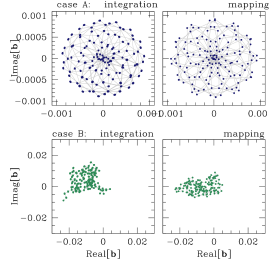
Figure 4.— Behaviour of the complex amplitudes (${\bf b}$, points), obtained using direct numerical integrations (left panels), and the simple toy-model (right panels), over $150$ passages. The top case is for $a_{0}=1$AU, $D_{p}=0.02$ AU and $P=P_{0}/1.1$, with $\Delta E_{\rm kick}/E_{0}\sim 4\times 10^{-6}$; while the bottom case is a mode with $P=1.1\times P_{0}$ that experiences a stronger kick ($\Delta E_{\rm kick}/E_{0}\sim 5\times 10^{-5}$) and is launched into diffusion. The toy-model is physically accurate, because using the same parameters, it reproduces both behaviour correctly.

I now proceed to construct a simple toy-model that yields the same mapping as the detailed numerics, one that is physically accurate. First, let us consider the magnitude and phase of individual kicks ($\Delta{\bf b}_{i}$).

The magnitude of individual kicks should be roughly constant in a given system ($|\Delta{\bf b}_{i}|=|\Delta b|$). Observing eq. (1), one realizes that the kick only depends on the orbital shape near periastron and the mode period. The latter is roughly conserved during the evolution, as the mode-orbit interactions do not absorb much of the orbital angular momentum, thereby conserving $D_{p}$. In this study, I take the mode period to be constant.

The phase of the $i$-th kick, $\Delta\theta_{i}$, depends only on the alignment between the pre-existing f-mode and the tidal potential at the time of kicking, which in turn depends on the angle the mode has rotated through in-between the kicks. Or, $\Delta\theta_{i}={\rm Mod}(\omega\Delta T,2\pi)$ with $\Delta T$ being the time between the $i-1$-th and $i$-th passages.

I now proceed to consider feedback onto the orbit. To produce a simple toy-model, I set $\Delta T$ to be the instantaneous orbital period. This then relates $\Delta T$ to the mode energy as,

$$\Delta T={P_{\rm orb,0}\left({{E_{\rm orb}}\over{E_{\rm orb,0}}}\right)^{3/2}\,,}$$ (13)

where $E_{\rm orb}=E_{0}+E$, with $E_{0}=GM_{*}M_{p}/2a_{0}$, and the mode energy $E=2\omega^{2}|b|^{2}M_{p}R_{p}^{2}$ (see eq. 4). The mapping model is now complete.

In Fig. 4, it is shown that such a simple model can accurately reproduce the outcomes of direct integrations. One can now proceed to use this toy-model to efficiently survey the parameter space, to determine how the diffusion threshold depends on various parameters, and to explain its origin.

3.2. Threshold I: $E_{\rm init}=0$

Starting from zero initial energy, the toy-model shows the same bifurcation in mode growth as the direct integration. Using the same parameters as those in Fig. 2 ($a=1$ AU, mode period $P\sim P_{0}$), one finds the boundary to be also at $\Delta E_{\rm kick}/E_{0}\sim 10^{-5}$ (Fig. 5).

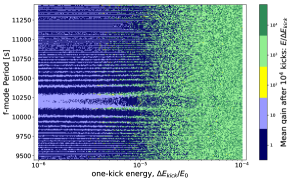
Figure 5.— The toy-model results. Here, we scan through a range of mode periods (vertical axis) and kick magnitudes (fractional energy gain, horizontal axis), starting from zero amplitudes for the mode. The color at each point represents the mean magnification in mode energy (mean energy divided by the one-kick energy, color bar on the right) over $10^{4}$ passages. Diffusive energy growth occurs when the kick magnitude is larger than about $10^{-5}$. Horizontal features correspond to modes with frequencies that are in resonance with the orbit. Here, the initial orbital period is 1 year (same as in Fig. 2).

What produces such a threshold? It turns out that even when the fractional kick energy is a very small number, its effect on the kick phase is not: it is amplified by the large number of oscillations in an orbital period. Above the observed threshold, the variation in the kick phase between successive kicks is,

$$\delta(\Delta\theta_{i})\sim{3\over 2}\left(\omega P_{\rm orb,0}\right){{\Delta E_{\rm kick}}\over{E_{0}}}\geq 0.3{\rm radian}\,.$$ (14)

This is now sufficiently large that the kicks can be considered to be un-correlated in phase. As a result,

$$|{\bf b}_{i}|^{2}=\sum_{i}|\Delta b|^{2}+2\sum_{i,j,i\neq j}\Delta{\bf b}_{i}\cdot\Delta{\bf b}_{j}\approx\sum_{i}|\Delta b|^{2}\,.$$ (15)

Or, the mode energy grows at a roughly linear rate,

$${{dE}\over{dt}}\approx{{\Delta E_{\rm kick}}\over{P_{\rm orb}}}\,.$$ (16)

In contrast, weaker exchanges do not scramble the kick phases and they are tightly correlated. Eq. (13) in this case acts as a restoring potential that limits the mode energy to within a few times the one-kick value.

The threshold energy depends on the mode period in a complicated way. Orbital resonances may be partially responsible for this. In the following study, I adopt a threshold of

$${{\Delta E_{\rm kick}}\over{E_{0}}} = {1\over{2\omega P_{\rm orb}}}$$ (17)

$$= 2\times 10^{-5}\left({{a_{0}}\over{1{\rm AU}}}\right)^{-3/2}\left({{P}\over{1.04\times 10^{4}\,\rm s}}\right)\,,$$

as a rough average.

3.3. Threshold II: $E_{\rm init}>0$

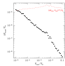
Figure 6.— The threshold one-kick energy for diffusion are plotted here in dots, as a function of the initial f-mode energy, while the geometric means of these two energies are shown as a red curve. The threshold value is obtained using the toy mapping model and is defined as, above this one-kick energy, $50\%$ of the system have diffused by more than $10^{4}\Delta E_{\rm kick}$ from their initial energies, after $10^{5}$ passages. Here, $P_{\rm orb,0}=1$ yr, and the mode period ranges from $P_{0}/1.1$ to $1.1\times P_{0}$. For comparison, the threshold kick at zero $E_{\rm init}$ lies at $\Delta E_{\rm kick}/E_{0}\sim 2\times 10^{-5}$.

Now consider the same problem but with an initial mode energy $E_{\rm init}\geq\Delta E_{\rm kick}$. Our toy-model shows that the threshold kick is now much reduced and lies at (Fig. 3),

$$\sqrt{{{\Delta E_{\rm kick}}\over{E_{0}}}\times{{E_{\rm init}}\over{E_{0}}}}\geq{1\over{2\omega P_{\rm orb}}}\,.$$ (18)

There is a simple explanation for this reduction of threshold. In the toy model, which involves the addition of a series of vectors that have equal lengths but different orientations, if the initial vector is placed well away from the origin, any new vector will introduce a much larger energy shift in the mode,

$$E_{i}-E_{i-1} \propto |{\bf b}_{i}|^{2}-|{\bf b}_{i-1}|^{2}$$ (19)

$$\approx 2{\bf b}_{i-1}\cdot\Delta{\bf b}_{i}+|\Delta{\bf b}_{i}|^{2}\,,$$

than if the initial vector is near the origin ($\sim|\Delta{\bf b}_{i}|^{2}$). This corresponds to a bigger change in the orbital period, and therefore a larger change in the kick phase the next time around. As a result, the threshold depends on the geometric mean of the initial and the one-kick energy.

Physically, the energy exchange between the orbit and the f-mode is enhanced when there is a pre-existing large-amplitude f-mode. This comes about because the f-mode can now perturb the orbit more efficiently (eq. 3), thereby affecting its own driving. In fact, the energy exchange accelerates as the f-mode gains energy.

4. Application to secular migration

I now return to the initial motivation for this work, the migration of hot Jupiters. We can now see how f-mode diffusion can effectively stall the secular migration, preventing the plants from being tidally disrupted, as well as how the orbits of these planets are subsequently circularized.

4.1. Stalling the secular migration

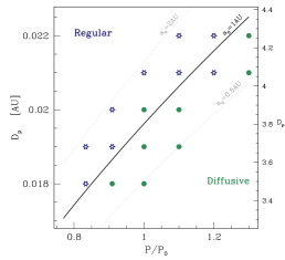
Figure 7.— The critical pericentre distance below which f-mode diffusion will occur, plotted here as a function of f-mode period (normalized by $P_{0}=1.04\times 10^{4}\,\rm s$) and applies when $E_{\rm init}=0$. The solid line represents the analytical scaling ( eq. 20) and the dots are results of orbit integration (filled green circles for diffusive and open stars for regular). The planet’s has an initial orbit of $a_{0}=1$ AU, and the two grey curves indicate how the critical distance is expected to change when it instead starts at $a_{0}=2$ and $0.5$ AU, respectively. The right axis is in units of tidal radius, where $r_{t}=(M_{*}/M_{p})^{1/3}R_{p}$.

Consider a migrating Jovian planet with an ever decreasing pericentre distance. Its f-mode is initially un-excited. Combining eqs. (9), (10) & (17), one finds that diffusive tidal evolution of this mode will kick in when

$$D_{p} \leq 0.02{\rm AU}\left({{R_{p}}\over{1.1R_{J}}}\right)^{2/21}\,\left({a_{0}\over{1{\rm AU}}}\right)^{5/42}\,\left({{Q_{n\ell}^{\prime}}\over{0.5}}\right)^{2/21}$$ (20)

$$\times\left({{P}\over{1.04\times 10^{4}\,\rm s}}\right)^{11/21}\,.$$

Notice that the $P$ here referes to the period of the prograde mode. The numerical version of this expression in plotted in Fig. 7, together with supporting evidences from our numerical integrations.

This is one of our key result. The critical $D_{p}$ has a very weak dependences on almost all parameters, and a weak dependence on the mode period. To make explicit the dependence on planet properties, one writes $P\approx P_{0}/(1+P_{0}/P_{\rm spin})$, where $P_{\rm spin}$ is the planet spin period (positive if spin aligns with the orbit), $P_{0}$ is the $\ell=2,m=0$ f-mode period and it scales with bulk planet properties as $P_{0}\approx 1.04\times 10^{4}\,\rm s(M_{p}/M_{J})^{-0.48}(R_{p}/1.1R_{J})^{2.1}$ (Le Bihan & Burrows, 2013). As such, eq. (20), measured in unit of tidal radius $r_{t}=R_{p}(M_{*}/M_{p})^{1/3}$, becomes

$${{D_{p}}\over{r_{t}}} \approx {3.8}\times(1+{P_{0}/P_{\rm spin}})^{-0.52}\,\left({a_{0}\over{1{\rm AU}}}\right)^{0.12}$$ (21)

$$\times\left({{R_{p}}\over{1.1R_{J}}}\right)^{0.19}\,\left({{M_{p}}\over{M_{J}}}\right)^{0.08}\,\left({{Q_{n\ell}^{\prime}}\over{0.5}}\right)^{0.09}\,,$$

The critical $D_{p}$ falls within a narrow range around $4$ tidal radii (also see Fig. 7). If one takes the definition of the Roche radius to be $R_{\rm Roche}=2.44r_{t}$, then the critical $D_{p}\sim 1.6R_{\rm Roche}$.

When the f-mode starts diffusing, orbital energy is quickly transferred to the internal oscillations and the orbit decays. This effectively decouples the planet from secular forcing by its companions. The rate of decay depends on $\Delta E_{\rm kick}$. The top example in Fig. 2 shows that it takes $\sim 400$ yrs for the orbit to decay from $1$ to $0.8$ AU. Since the strength of secular coupling goes down with $a$ ($\propto a^{3}$ for quadrupole coupling), and because secular forcing depends sensitively on the concordances among different secular frequencies (which depend on $a$ nonlinearly), such an orbital decay substantially reduces the secular forcing and prevents the planet orbit from getting even closer to the star. To further strengthen this point, one notes that since the one-kick energy scales with $D_{p}$ as $D_{p}^{-21}$, a minute drop in $D_{p}$ is sufficient to overcome any strength of secular forcing, even if the diffusion is initially too slow to stall the migration. The planet is safely parked around that predicted in eq. (21).

The f-mode also introduces an apsidal advance that can help to decouple the planet from secular forcing. It is found numerically that the precession rate is a few times higher than that predicted using equilbrium tide theories (Sterne, 1939; Smeyers et al., 1991). But it has a weaker dependence on $D_{p}$ as $D_{p}^{-5}$, so it helps to stall migration with weak secular forcing (e.g., the case of HD 80606), but the orbital decay is a more fail-proof mechanism.

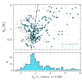
Figure 8.— The stalling distances of hot Jupiters with known radii and masses. In the top panel, the horizontal axis is the periastron distance when $e=0.98$, plotted in unit of the tidal radius, while the vertical axis is planet mass (in unit of Jupiter mass). The grey open circles are obtained using planets’ current observed radii, while the blue solid ones are obtained by assuming $R_{p}=1.1R_{J}$. The thick black line is the theoretical threshold for f-mode diffusion (eq. 21), assuming $P=1.04\times 10^{4}\,\rm s$ and zero spin. While low-mass hot Jupiters cluster around this prediction, high mass ones are much more spread out. The bottom panel shows the corresponding histograms. There is a strong pile-up just below 4 $r_{t}$, as predicted, if planets are indeed $\sim 1.1R_{J}$ in radius when they were migrated.

One can now compare the critical distance against the current positions of known hot Jupiters. Most of them have now near zero eccentricities, so at high eccentricities, they should satisfy $D_{p}(e\approx 1)=a(e\approx 0)/2$. I plot these values against planet masses in Fig. 8, and find that most the observed hot Jupiters satisfy $D_{p}$$(e\approx 1)$ $\sim 3r_{t}$ if we adopt their current (inflated) radii, and $D_{p}\sim 4r_{t}$ if we assume instead that during migration, their radii $R_{p}=1.1R_{J}$.

This is expected. The progenitors of hot Jupiter likely possess the same orbital distribution as the cold Jupiters found today by radial velocity surveys, namely, a precipitous rise just outside $a=1$AU and a gradual fall further out. So eq. (21) predicts $D_{p}(e\approx 1)\sim 3.8r_{t}$ for non- or slowly-spinning planets, and slightly smaller values for rapidly spinning planets. Moreover, there should be a sharp pile-up around this value due to the weak dependence of critical $D_{p}$ on all relevant parameters. As Fig. 8 shows, the observed spread around $4r_{t}$ is indeed narrow for planets less massive than Jupiter, but appears to be much broader for higher mass planets. The model here could not account for this latter behaviour but I note that for these higher mass planets, tidal excitation in stars may become more relevant (see, e.g. Ivanov & Papaloizou, 2004; Barker & Ogilvie, 2010).

4.2. Towards Orbital Circularization

Now consider the Jupiter after its secular migration has been stalled. It now resides on a high eccentricity orbit with $D_{p}$ near the original threshold, largely independent of the secular forcings. As the f-mode gains energy, the nonlinear criterion (eq. 18) takes hold. This now facilitates the eventual circularization – as the orbit decays and $D_{p}$ gradually rises, the one-kick energy drops precipitously. The nonlinear threshold reduces the one-kick energy required for diffusion and allows the planet to continue on its way to circularization.

We define another energy scale for the f-mode, $E_{1}$. Let $\Delta r$ be its surface radial displacement at the equator, we define

$$E_{1}=E(\Delta r=R_{p})\sim{0.1{{GM_{p}^{2}}\over{R_{p}}}}\sim 3\times 10^{42}\,\rm erg\,.$$ (22)

For comparison, the orbital energy at $a=1$ AU is $9\times 10^{42}\,\rm erg$. Here, I restrict $E\leq E_{1}$ and discuss the nonlinear evolution of the f-mode in a later section.

Let us assume that the earlier evolution has endowed the f-mode with a non-zero initial energy that is a fraction of $E_{1}$. As is shown in Fig. 9, the minimum distance the planet can reach via diffusive evolution depends on this fraction. Starting from a high-eccentricity orbit with $D_{p}=0.02$ AU, if the energy fraction is $10^{-2}$, the planet can continue to experience diffusive tidal evolution (satisfying eq. 18) until its orbit has shrunk to $a=0.13$ AU ($e=0.83$); and if the fraction is raised to $10^{-1}$, the evolution can proceed further till $a=0.09$AU ($e=0.73$).

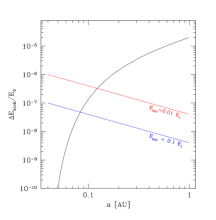
Figure 9.— The reach of diffusive tidal evolution. Here, starting from $D_{p}=0.02$ AU and $a=1$ AU, the planet moves inward on a trajectory of constant angular momentum (horizontal axis is the semi-major axis, in AU). The vertical axis is the one-kick energy it is expected to receive along this trajectory and it drops precipitously during the evolution (black curve), as a result of a slight increase in $D_{p}$. This energy is normalized by the local orbital energy ($E_{0}=GM_{*}M_{p}/2a$), and $P=P_{0}$. The two coloured curves indicate the minimum one-kick energy required to cause tidal diffusion, when the f-mode energy takes on two initial values ($0.01$ or $0.1E_{1}$, where $E_{1}$ corresponds to unity radial displacement at the surface). In both cases, the diffusive evolution can be sustained inward till $a\sim 0.1$ AU. Here, the orbit integral $K_{\ell m}$ is calculated as in eq. (8).

The change in orbital energy between the above final ($a\sim 0.1$ AU) and initial orbits ($a=1$ AU) exceeds the binding energy of the planet by a factor of a few. Can a single f-mode carry the planet inward for such a large distance?

In Fig. 10, I present a scenario to illustrate how I believe this is accomplished. The planet is initially placed at an orbit with $a=1$AU, $D_{p}=0.02$AU ($e=0.98$). Its f-mode starts random-walking and this continues until its amplitude has reached unity. At this point, nonlinearity is important (§5.2). Here, I simply specify that the mode energy be instantaneously removed, leaving a small residual energy, and that there be no changes in the planet’s properties (radius, mass, spin rate). Thanks to the residual energy, the f-mode remains diffusive, and is soon undergoing another nonlinear damping. Within an astronomically short time (a few $10^{4}$ yrs), the orbit has decayed to $a\sim 0.2$ AU, or an eccentricity of $e\sim 0.9$. Evolution practically stalls after reaching this point.

These stalling distances lie twice above our analytical predictions ($a=0.1$ AU, Fig. 9). The reason may be observed in the right-hand panel of Fig. 1 – by the time the planet has migrated to these distances, the parabolic approximation for the orbit integral is no longer valid, it is instead dominated by a series of resonances. Our simple treatment should fail in this regime.

If our scenario is correct, there are two immediate implications, one relates to the effective tidal $Q$ number, the other relates to the observed absence of very high eccentricity planets.

The amount of energy transferred to the f-mode per orbit is $\sim\sqrt{E\Delta E_{\rm kick}}$, where $E$ is the mode energy (eq. 19). To re-cast our results using the so-called tidal-quality factor ($Q$), we invoke the following expression for tidal orbital decay, valid for high eccentricity orbits (MacDonald, 1964; Goldreich et al., 1989),

$${1\over a}{{da}\over{dt}}=-{{21}\over{64}}{n\over\mu}{{aR_{p}^{5}}\over{D_{p}^{6}}}{{k_{2}}\over{Q}}\,,$$ (23)

where $n$ is the orbital frequency, $\mu=M_{p}/M_{*}$, and $k_{2}$ is the tidal Love number which I take to be $0.3$. Combined with eq. (5), eq. (9) and eq. (22), this yields

$$Q = {{42\pi}\over{64}}{1\over\mu}{{aR_{p}^{5}}\over{D_{p}^{6}}}{{k_{2}E_{0}}\over{\sqrt{E\Delta E_{\rm kick}}}}$$ (24)

$$\approx 73\sqrt{{E_{1}}\over{E}}\left({{R_{p}^{3}}\over{M_{p}}}\times{{M_{*}}\over{D_{p}^{3}}}\right)^{3/2}\left({{K_{\ell m}}\over{0.006T_{\rm peri}}}\right)^{-1}$$

$$\approx 0.5\times\left({{E\over{10\%E_{1}}}}\right)^{-1/2}\left({{D_{p}}\over{0.02{\rm AU}}}\right)^{4.5}\left({{P}\over{1.04\times 10^{4}\,\rm s}}\right)^{-6}\,,$$

where I have scaled the f-mode energy $E$ by typical values observed in Fig. 10.

Such a small $Q$ factor differs from the common conception that $Q\sim 10^{5}$ for Jovian planets, a conception that comes from constraints on the Gallilean satellites which move on nearly circular orbits (Goldreich & Soter, 1966). It makes sense, however, on hind sight: the f-mode is the equilibrium tide, or most of it; and the f-mode diffusion moves energy in such a way that of order the equilibrium tide energy is effectively absorbed by the planet after every passage, though the true dissipation (nonlinear breaking) really only sets in when the mode is at unity amplitude.

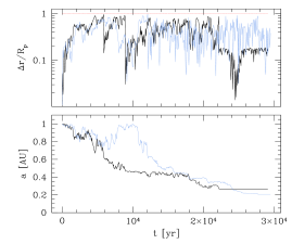
Figure 10.— Diffusive tidal evolution involving only one f-mode. A Jovian planet (with $P=P_{0}$) is initially placed at $a=1$AU and $D_{p}=0.02$ AU ($e=0.98$). The top panel shows the fractional radial displacement, measured at the surface of the planet, and the bottom panel the semi-major axis of the orbit. Whenever the diffusion has grown the f-mode to unity amplitude (red line), I prescribe the code to remove $99\%$ (the solid black curve, or $90\%$ for the dashed blue curve) of the mode energy instantaneously, down to $1\%E_{1}$ (or $10\%E_{1}$). After $\sim 10^{4}$ yrs, the planet orbit has tidally circularized to $a\sim 0.2$. After this point, diffusion is inhibited (Fig. 9) and the tidal evolution stalls.

Fig. 10 shows that, starting from an eccentricity of $e=0.98$, a Jovian planet can circularize its orbit to $e<0.9$ within a few $10^{4}$ years. Let this timescale be $10^{5}\,\rm yrs$ to be on the conservative side. One can estimate the number of super-eccentric planets ($e>0.9$) one expects in the Kepler sample of $200,000$ stars. First, assume that about $1\%$ of the stars could eventually own a hot Jupiter, based on the observed frequency of hot Jupiters. If the event that makes them occur relatively uniformly during the stars’ lifetimes ($\sim 5$ Gyrs), the number of super-eccentric Jupiters should be

$$N_{\rm e>0.9}\approx 200,000\times 1\%\times{{10^{5}\,\rm yrs}\over{5\times 10^{9}\,\rm yrs}}\sim 0.04\,.$$ (25)

This value is further reduced when one considers the geometric probability of a planetary transit.

This explains the observed deficit of such planets (Dawson et al., 2015), despite the arguments presented in Socrates et al. (2012). Tidal dissipation at very high eccentricity proceeds efficiently, likely far more efficient than when the planet is less eccentric. About the latter we still have no good first-principle theory.

5. Miscellaneous

Here, I justify a number of assumptions in our model, discuss the nonlinear behaviour of the f-mode, the impacts of nonlinear damping on the planet, and compare our results with previous studies.

5.1. Assumptions

I only consider one $\ell=2,m=-2$ f-mode. The other modes contribute at the percent level and can be safely ignored (also see Mardling, 1995). This is due to a number of factors: the tidal potential drops off for higher multiples ($\ell$); the tidal integral, $Q^{\prime}_{n\ell}$, drops off with the mode’s radial order; the orbit integral, $K_{\ell m}$, drops off steeply with decreasing mode periods. Relatedly, when the f-mode is strongly excited, it could help make the other modes to go stochastic, However, since the one-kick energy is the largest for the f-mode, it still diffuses the fastest. As a result, it dominates the orbital evolution.

I ignore linear dissipation on the f-mode. The dominant viscosity in a fully convecting planet is turbulent viscosity. But since the convection over-turn time ($\sim$ yr) is some $4000$ times longer than the f-mode period, the effective damping time is $\sim 4000^{2}\sim 10^{7}$ yrs (Goldreich & Nicholson, 1977). This is far longer than the longest timescale of interest here, $\sim 10^{4}$ yrs.

In our model, I assume the planet bulk properties (radius, mass, spin rate) remain constant throughout the evolution, despite the repeated nonlinear breaking of the f-mode. I give arguments to support this in §5.2.

I have ignored tidal response in the star. To estimate the relative importance of the stellar f-mode, let us swap the subscripts for the star and the planet in eq. (5), to find that, for the same body density and a similar mode period, the f-mode energy gain in the star is roughly $R_{p}/R_{*}\sim 1/10$ times of that in the planet, for a $1-M_{J}$ planet. This ratio is less extreme for more massive planets. Solar gravity-modes, on the other hand, may in fact be more important than the f-mode – they are coupled to the tidal potential less strongly (smaller $Q^{\prime}_{n\ell}$), but their lower frequencies may enhance $K_{\ell m}$ (Ivanov & Papaloizou, 2004). This study falls short of investigating this and this may explain our failure to reproduce the orbits for the high mass planets in Fig. 8.

5.2. Nonlinear Evolution

The gravitational binding energy of a Jovian planet,

$${{GM_{J}^{2}}\over{R_{J}}}\sim 4\times 10^{43}\,\rm erg\,,$$ (26)

is comparable to the magnitude of its orbital energy at a few AU,

$$E_{0}=|E_{\rm orb}|=\left|-{{GM_{\odot}M_{J}}\over{2a}}\right|\sim 10^{43}\,\rm erg\,\times\left({a\over{1{\rm AU}}}\right)^{-1}\,.$$ (27)

This suggests the importance of internal oscillations in modifying the orbit. It also suggests that the internal oscillations can acquire enough energy to go nonlinear. The evolution subsequent to this is uncertain. I give my educated guess below.

Can f-mode be saturated at a very low amplitude, much below unity? Let us consider mode coupling to transport energy out of the f-mode. In a fully convective planet like Jupiter, gravity-modes do not exist, and inertial-modes lie too low in frequency (unless the planet is near critical spin). As a result, the only 3-mode coupling for the f-mode involves it (twice) and another f- or p-modes at twice its frequency. However, the sparse spectrum of these latter modes implies that this coupling is typically far from resonance, and the energy transfer rate is limited unless the f-mode has reached order unity amplitude ($\Delta r\sim R_{p}$), by which time 4-mode coupling may be just as important as 3-mode coupling. This is analogous to the situation in Cepheids and RR Lyrae pulsation where the over-stable f-mode pulsation grows to unity amplitudes.

What happens when the f-mode reaches order unity amplitude? Both mode coupling and wave breaking are possibilites to convert its energy into heat. Kumar & Goodman (1996) studied the 3-mode coupling by solving the equation of fluid motion, with the f-mode acting as an inhomogeneous forcing term at twice its own frequency. They found that energy is taken out of the f-mode at a rate comparable to its own frequency when $E\sim E_{1}$. Moreover, they found that the forced response peaks near the surface ($<100$ bar), and may itself be prone to further nonlinear damping. Another study of note is that by Kastaun et al. (2010). Using a general relativistic hydro-code to study a star undergoing a large f-mode oscillation, in the context of rapidly spinning neutron stars, they reported that when the f-mode has unity amplitude, the stellar surface is gradually distorted away from a sinusoidal waveform, leading to steepening and wave breaking, analogous to the breaking of ocean waves. In either of these calculations, the f-mode energy excites near surface phenomenon, and energy dissipation occurs near the surface, possibly within a few scale heights of the photosphere.

When the f-mode is (nonlinearly) dissipated, what happens to the planet’s structure and spin? The rapid dissipation of the f-mode in a few oscillation timescale gives rise to a luminosity of $L\sim 10^{37}\,\rm erg/\,\rm s$, outshining even the host star. This is much beyond the planet’s Eddington luminosity ($\sim 10^{35}\,\rm erg/\,\rm s$), and is much more than can be carried out by convection or radiative diffusion. As a result, it must lead to envelope expansion and mass loss. But since all the nonlinear dissipation occurs at the low density, superficial region of the planet, the mass loss rate is not significant, and the heated layer can cool within a short amount of time. More importantly, it is hard to transport entropy up the temperature gradient toward the planet interior, so one expects little impact on the internal entropy. The radius of the planet at constant entropy, on the other hand, goes as $R\propto M^{0}$, as the polytropic index $n\sim 1$ under the combined effect of electron degeneracy and Coulomb force. So, to first order, one can assume that the planet’s radius hardly changes. The spin evolution should also be impacted by the mode of energy dissipation. In the case where f-mode dissipation only occurs at the surface, the angular momentum it carries will also likely be lost to the expanding envelope and is quickly removed. In this case, there is little spin evolution in the planet interior. Both these considerations justify, to some degree, my simplification of keeping a constant f-mode period.

After nonlinear damping is finished, it is likely that the f-mode still retains a fraction of its former energy. In particular, oscillations in the central region is still very linear ($\xi_{r}\ll R_{p}$) and may not be completely removed. This motivates us, in Fig. 10, to assume that a small fraction remains to seed the subsequent random-walk.

Would the now severely distended planet undergo tidal disruption? Sridhar & Tremaine (1992) obtained that the threshold for tidal shredding of an incompressible, homogeneous sphere on parabolic orbit lies at $1.69r_{t}$. At a distance of $4r_{t}$, the planet is safe from tidal disruption even if one assumes its radius is diluted by a factor of 2 by pulsation.

In summary, as the planet’s orbit decays, the f-mode repeatedly breaks near the planetary surface, depositing energy and angular momentum in the top layers, possibly driving a wind. However, the bulk of the planet may feel little impact. One does not expect the planet to be thermally ablated. But detailed investigation is required to assess the damage.

An additional concern arises when the mode amplitude becomes very large. Mode period may be shifted nonlinearly and the pulse shape may become anharmonic. We have not included these into our consideration and they may impact the long-term evolution.

5.3. Comparing with previous studies

Mardling (1995) studied the chaotic diffusion under extreme tidal forcing. She used numerical simulations to delineate the boundary between chaos and regular behaviour, for a system of two equal mass, $n=1.5$ polytropes. In particular, she showed that a highly eccentric orbit at $e=0.98$ (the fiducial case considered here) can kick start tidal diffusion when $D_{p}\leq 4.2r_{t}$, slightly larger than our prediction of $3.8r_{t}$. The difference may be due to our different assumptions on the model structure. Furthermore, she demonstrated numerically that a non-zero initial energy can boost diffusion (her Fig. 15). We provide an explanation for this effect, as well as present a quantitative criterion.

Ivanov & Papaloizou (2004) was the first to explain the physics behind the f-mode random-walk, using analytical arguments and a toy-model. Their study is the closest to ours as they also focussed on a Jovian planet around a solar-type star. Their central result is their eq. (107) where they showed that, for a certain value of $D_{p}$, there is a minimum $a_{\rm st}$ above which the tidal dynamics is stochastic. Substituting our expression for $K_{\ell m}$ into their notation, one obtains that $a_{\rm st}\propto D_{p}^{-42/5}P^{-22/5}$, reproducing the scalings in our eq. (20), and with a similar normalization.

A study recently appeared while I was preparing the manuscript. Vick & Lai (2017) adopted the 2-D mapping approach to investigate the same dynamics as we study here. Their Fig. 1 is similar to our Fig. 5. They have also generalized the model to include effects of mode dissipation, resonances and gravity-modes. These are important for stars (the case they consider) but not for Jovian planets.

Lastly, Papaloizou & Ivanov (2005); Ivanov & Papaloizou (2007) considered the stochastic excitation of inertial modes, in lieu of f-modes studied here. They calculated that a couple low-order inertial modes can couple to the tidal potential sufficiently strongly (also see Fig. 2 in Wu, 2005), that they can potentially supplant the f-modes, for cases where the peri-centre distance is larger than the values considered here. This occurs because the longer periastron passage time weakens the orbit integral for f-modes, while inertial modes may not suffer as much, if one assumes that the rotation frequency remains comparable to $1/T_{\rm peri}$. This may be another venue for tidal circularization.

6. Conclusion

In this work, I use both direct numerical integration and a toy-model to investigate the tidal evolution of a Jovian planet on a highly eccentric orbit around its host star. The findings here allow us to overcome three of the theoretical weaknesses in dynamical migration for hot Jupiters, and boost the overall prospects for dynamical migration.

I show that, when the planet’s pericentre dips below $4$ tidal radii, one of its f-modes starts gaining energy stochastically. Because there is more phase space for the f-mode at high energy, and because the orbit and the f-mode try to reach energy equi-partition, the f-mode diffusively grows towards unity amplitude. The growth of the f-mode is accompanied by the decay of the orbit. So a Jupiter that is secularly perturbed to high eccentricity will be stalled and dynamically decoupled from its perturbers when its pericentre distance reaches $\sim 4$ tidal radii. They are safely parked where they are observed today, without suffering the fate of tidal disruption.

One of the ’accepted’ examples for secular migration is HD 80606 (Wu & Murray, 2003). At its current orbit of $D_{p}=0.03$ AU and $e=0.983$, it should never have crossed inward of $D_{p}=0.029$ AU, or $11r_{t}$ ($M_{p}=4M_{J},R_{p}=0.9R_{J}$). This is too far for f-mode diffusion. However, if this planet is indeed migrated inward by its remote stellar companion ($\sim$ a thousand AU) as suggested, the weak secular perturbation from the companion can be easily stalled at the observed distance by tidal and secular precessions (Wu & Murray, 2003), without the need to invoke diffusive tidal evolution.

One of the new insights in this work is that mode diffusion can occur at a lower threshold when the f-mode has some non-zero energy to start with (also see Mardling, 1995). This insight is important for transporting the planet all the way from a few AU to a small fraction of an AU. In our simulations, we model this by assuming that whenever the f-mode nonlinearly damps, a fraction of the initial energy is retained to seed the next episode of random-walk. These simulations show that, within a few $10^{4}$ years, the planet drops its eccentricity from near unity to $0.9$. We therefore do not expect to see any super-eccentric Jupiters ($e>0.9$) among the $200,000$ stars observed by the Kepler mission. More strikingly, the process discussed here achieves an effective tidal $Q\sim 1$, in an otherwise invisid planet. This helps explain how the planet dissipates the tide, without invoking any ad hoc weak friction.

To emphasize the last point, I note that although the planet’s orbit decays and circularizes due to f-mode diffusion, these changes are temporary and occur without any explicit dissipation in the system. It is only when the f-mode is nonlinearly dissipated, either through mode-coupling or wave breaking, these orbital changes are perpetuated and tidal circularization becomes time irreversible.

Our story fails, however, after $a\sim 0.2$ AU. What mechanism is capable of further circularizing the planet to the nearly zero eccentricity we see today? Can the residual energy in the f-mode be again useful? If the tidal process proceeds much more slowly in the later stage, are there any observational consequences (e.g., warm jupiters from stalled circularization)?

Lastly, the fate of a tidal planet under the massive amount of energy deposition need not be dire. I argue that f-mode dissipation occurs exclusively near the surface. As the f-mode energy is converted into heat, this should lead to envelope expulsion but should keep the planet interior largely intact.

References

- Barker & Ogilvie (2010) Barker, A. J., & Ogilvie, G. I. 2010, MNRAS, 404, 1849
- Dawson et al. (2015) Dawson, R. I., Murray-Clay, R. A., & Johnson, J. A. 2015, ApJ, 798, 66
- Ford et al. (2001) Ford, E. B., Havlickova, M., & Rasio, F. A. 2001, Icarus, 150, 303
- Gingold & Monaghan (1980) Gingold, R. A., & Monaghan, J. J. 1980, MNRAS, 191, 897
- Goldreich et al. (1989) Goldreich, P., Murray, N., Longaretti, P. Y., & Banfield, D. 1989, Science, 245, 500
- Goldreich & Nicholson (1977) Goldreich, P., & Nicholson, P. D. 1977, Icarus, 30, 301
- Goldreich & Soter (1966) Goldreich, P., & Soter, S. 1966, Icarus, 5, 375
- Gudkova & Zharkov (1999) Gudkova, T. V., & Zharkov, V. N. 1999, Planet. Space Sci., 47, 1211
- Guillochon et al. (2011) Guillochon, J., Ramirez-Ruiz, E., & Lin, D. 2011, ApJ, 732, 74
- Hamers et al. (2017) Hamers, A. S., Antonini, F., Lithwick, Y., Perets, H. B., & Portegies Zwart, S. F. 2017, MNRAS, 464, 688