Comparing reverse complementary genomic words based on their distance distributions and frequencies

Abstract

In this work we study reverse complementary genomic word pairs in the human DNA, by comparing both the distance distribution and the frequency of a word to those of its reverse complement. Several measures of dissimilarity between distance distributions are considered, and it is found that the peak dissimilarity works best in this setting. We report the existence of reverse complementary word pairs with very dissimilar distance distributions, as well as word pairs with very similar distance distributions even when both distributions are irregular and contain strong peaks. The association between distribution dissimilarity and frequency discrepancy is explored also, and it is speculated that symmetric pairs combining low and high values of each measure may uncover features of interest. Taken together, our results suggest that some asymmetries in the human genome go far beyond Chargaff’s rules. This study uses both the complete human genome and its repeat-masked version.

1 Introduction

The analysis of DNA sequences is an extremely broad research domain which has seen several new approaches over the last years. One of these newer approaches is the study of distance distributions of genomic words. A genomic word, also called an oligonucleotide, is a sequence of nucleotides which are represented by the letters $\{A,C,G,T\}$. In DNA segments, the inter-word distance is defined as the number of nucleotides between the first symbol of consecutive occurrences of that word [2, 16]. For instance, in the DNA segment $A\underline{CG}T\underline{CG}ATC\underline{CG}TG\underline{CG}\,\underline{CG}$ the inter-$CG$ distances are (3,5,4,2). For each word, all of its inter-word distances in the genome sequence can be counted and aggregated into a distance distribution, which contains the frequency of each distance. These distributions provide a characterization of genomic words which can be studied using statistical techniques for probability density functions.

In this paper we are particularly interested in the study of symmetric word pairs. A symmetric word pair is formed by a word $w$ and its reverse complement $\bar{w}$, which is the word obtained by reversing the order of the letters and interchanging the complementary nucleotides $A\leftrightarrow T$ and $C\leftrightarrow G$. For instance, the reverse complement of $w=AAGT$ is $\bar{w}=ACTT$, and together they form the symmetric pair $\{w,\bar{w}\}$. The interest in these pairs stems from Chargaff’s second parity rule which implies that within a strand of DNA the number of complementary nucleotides is similar [9]. One potential explanation postulates that this phenomenon would be an original feature of the primordial genome, the most primitive nucleic acid genome, and the preservation of strand symmetry would rely on evolutionary mechanisms [18]. Symmetric word pairs can occur in a genome through recombination events such as duplications, inversions and inverted transpositions [7, 6]. These segments have been associated with specific biological functions, namely, replication and transcription, and major evolutionary events including recombination and translocations. Also, the potential to form secondary DNA structures can cause the genome instability observed in some diseases [11].

Chargaff’s second parity rule has led to the natural question whether this also holds for symmetric word pairs. This question has been answered to a certain extent in the existing literature [1, 3, 5, 7], as it has been observed that even for long DNA words in several organisms, including the human genome, the frequency of a word is typically (but not always) similar to that of its reverse complement. However, two words with the same frequency in a sequence may exhibit very distinct distance distributions along that sequence. This leads to the natural follow-up question: do symmetric word pairs have similar distance distributions?

Tavares et al. [16] addressed this question for words of length $k\leq 5$ in the human genome. Adopting a whole-genome analysis approach, the discrepancy between distance distributions was evaluated using an effect size measure. The authors concluded that the dissimilarity between the distributions of symmetric word pairs of this length was negligible. The authors also reported that for each word $w$, the distance distribution nearest to the distance distribution of $w$ is most often that of $\bar{w}$, the reverse complement of $w$.

As an example, Figure 1 shows the distance distribution of the word $w=GGGAGGC$ in the human genome. Its peaks correspond to three distances that occur much more often than others. In this example the distance distribution of the reverse complement $\bar{w}=GCCTCCC$ is extremely similar.

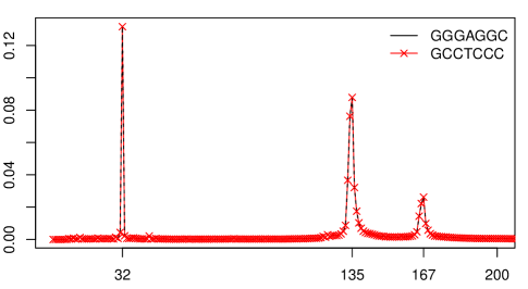
Figure 1: Distance distribution of the genomic word $w=GGGAGGC$ and of its reverse complement $\bar{w}=GCCTCCC$ in the human genome (adapted from [16]).

In order to study differences between distance distributions, a new dissimilarity measure was proposed by Tavares et al. [17]. Based on the gaps between the locations of their peaks and the difference between the sizes of these peaks, the peak dissimilarity becomes high when the distributions have very different peaks, or when one distribution has strong peaks and the other does not. In this article we extend their work in two ways. First, we compare the peak dissimilarity with two earlier dissimilarity measures and argue for its superiority in the analysis of distance distributions between symmetric word pairs. Secondly, we combine the peak dissimilarity with information about the frequencies of the word and its reverse complement to improve the identification of atypical genomic word pairs. We also draw a comparison between the observed distribution and the expected distribution under randomness. Using these techniques we detect several atypical word pairs, which we annotate by identifying the chromosomes and genes where their differences are most pronounced.

The paper is organized as follows. In Section 2 we describe measures of the discrepancy between frequencies and distance distributions, including the peak dissimilarity. Section 3 compares the behavior of these dissimilarity measures in our particular research problem. Section 4 identifies and investigates the symmetric word pairs that are most and least dissimilar, using both their frequencies and their distance distributions. It also explores how well the results hold up in a masked sequence. Section 5 concludes.

2 Measures of dissimilarity

2.1 Discrepancy between word frequencies

To measure the discrepancy between the total absolute frequencies of reverse complementary words $w$ and $\bar{w}$, we count all occurrences of each word along the DNA sequence. The number of times $w$ occurs is denoted as $n^{w}$, and that of $\bar{w}$ is $n^{\bar{w}}$. Under the null hypothesis that the true underlying probabilities of $w$ and $\bar{w}$ are equal, the expected frequency of $w$ is $e=(n^{w}+n^{\bar{w}})/2\;$. The Pearson residual [4] of $w$ is then given by $(n^{w}-e)/\sqrt{e}\;$. The absolute Pearson residual (APR) of $w$ is thus

$$\mbox{APR}(w)=\frac{|n^{w}-e|}{\sqrt{e}}=\frac{|n^{w}-n^{\bar{w}}|}{\sqrt{2(n^{w}+n^{\bar{w}})}}\;\;.$$ (1)

Note that $\mbox{APR}(w)=\mbox{APR}(\bar{w})$ and that $2\mbox{APR}^{2}(w)$ equals the usual chi-squared statistic for testing the equality of the underlying probabilities.

2.2 Dissimilarity measures for distance distributions

Assuming that the DNA sequence is read through a sliding window of word length $k$, the inter-word distance sequence is defined as the differences between the positions of the first symbol of consecutive occurrences of that word. For instance, the inter-$CG$ distances sequence in the DNA segment $CGTACGCGACG$ is (4,2,3). The distance distribution of $w$, denoted by $f^{w}$, gives the relative frequency of each distance, i.e. the number of times a certain distance occurs divided by the total number of occurrences of the word $w$.

The word structure influences the distance distribution, as some distances from 1 to $k$ may be absent. As an example, note that the inter-$AAA$ distance can be equal to one, but cannot be two or three. So, for words of length $k$ we will only consider distances greater than $k$.

We now wish to compare the distance distribution of each word $w$ with the distance distribution of $\bar{w}$. For this we describe three dissimilarity measures, two of which have been used for a long time and one is new.

2.2.1 Euclidean distance

The Euclidean distance is a standard tool which is also used between distributions. In our situation, the discrete probability distributions $f^{w}$ and $f^{\bar{w}}$ have the same domain. The word ‘discrete’ refers to the domain, as the distances are always integers. The probabilities (i.e. frequencies) of a distance $i$ are denoted as $p_{i}=f^{w}(i)$ and $q_{i}=f^{\bar{w}}(i)$. Then the Euclidean distance $D_{E}(f^{w},f^{\bar{w}})$ is obtained by summing the squares of the frequency differences:

$$D_{E}(f^{w},f^{\bar{w}})=\sqrt{\sum_{i}(p_{i}-q_{i})^{2}}$$ (2)

2.2.2 Jeffreys divergence

The Kullback-Leibler divergence [13] between $f^{w}$ and $f^{\bar{w}}$ is given by

$$D_{KL}(f^{w},f^{\bar{w}})=\sum_{i}p_{i}\log(p_{i}/q_{i})$$

where the $0\log 0=0$ convention is adopted. The Kullback-Leibler divergence stems from information theory. It is always nonnegative and becomes zero when the distributions are equal, and it is widely used as a divergence measure between distributions. But it is not symmetric, as $D_{KL}(f^{w},f^{\bar{w}})$ need not equal $D_{KL}(f^{\bar{w}},f^{w})$. Therefore we will use a symmetrized version called the Jeffreys divergence [12]:

$$D_{J}(f^{w},f^{\bar{w}})=D_{KL}(f^{w},f^{\bar{w}})+D_{KL}(f^{\bar{w}},f^{w})\;\;.$$ (3)

Note that $D_{J}$ is not well defined if some $p_{i}$ or $q_{i}$ are zero. In practice this can be avoided by replacing the zero values by a small positive value. The Jeffreys divergence $D_{J}$ is a semimetric, meaning that it is symmetric, nonnegative, and reduces to zero when the two distributions are identical.

2.2.3 Peak dissimilarity

The distance distributions $f^{w}$ and $f^{\bar{w}}$ may present several peaks, i.e., distances with frequencies much higher than the global tendency of the distribution, as we saw in Fig. 1. To describe the recently proposed peak dissimilarity [17] we go through three steps.

1. Identifying peaks. To determine peaks we slide a window of fixed width $h$ along the domain of the distribution. In each such interval of width $h$ we average the absolute values of the differences between successive frequencies, and call the result the size of the peak on that interval. The peak’s location is defined as the midpoint of the interval. The strongest peak is then determined by the interval with the highest size. For the second strongest peak we only consider intervals that do not overlap with the first one, and so on.

The bandwidth $h$ is a tuning parameter which controls the number of consecutive frequencies that are aggregated in a region. There is no best bandwidth, and different bandwidths can reveal different features of the data. To illustrate the effect of $h$ on peak identification, consider the distance distribution of the word $w=GGGAGGC$ in Figure 1 which has a local maximum at distance 135. When $h\leq 3$ the region around distance 135 gives rise to two intervals with high peak size. However, when $h\geq 4$ these high frequencies are combined into a single peak.

2. Dissimilarity between two peaks. To measure the dissimilarity between two peaks we take into account the difference between their sizes and between their locations. Consider the distance distributions $f^{w}$ and $f^{\bar{w}}$ which are defined on the same domain with length $R$. Let $t^{w}_{i}$ be a peak of $f^{w}$ with location $l_{i}$ and size $v_{i}$ and let $t^{\bar{w}}_{j}$ be a peak of $f^{\bar{w}}$ with location $\bar{l_{j}}$ and size $\bar{v_{j}}\;$. To measure the dissimilarity between these peaks we propose to use

$$d(t^{w}_{i},t^{\bar{w}}_{j})=\left(\frac{|l_{i}-\bar{l_{j}}|}{R}+1\right)\left(\frac{|v_{i}-\bar{v_{j}}|}{\min\{v,\bar{v}\}}+1\right)-1$$ (4)

where $v$ and $\bar{v}$ are the highest peak sizes observed in each distribution. If the peaks have the same location the dissimilarity is reduced to a relative size difference $|v_{i}-\bar{v_{j}}|/\min\{v,\bar{v}\}$, and if they have the same size it is reduced to a relative location difference $|l_{i}-\bar{l_{j}}|/R$. The denominator $\min\{v,\bar{v}\}$ yields a high dissimilarity when one distribution has strong peaks and the other doesn’t.

3. Peak dissimilarity between two distributions. To measure the dissimilarity between two distributions we compare their $n$ strongest peaks, for fixed $n$. We propose

$$D_{P}(f^{w},f^{\bar{w}})=\min_{\pi\in\mathcal{P}_{n}}\{\,\sum_{i=1}^{n}d(t^{w}_{i},t^{\bar{w}}_{\pi(i)})\,\}$$ (5)

where $\pi$ is a permutation of the indices $i=1,\ldots,n$ meaning that $\pi(i)$ is the image of $i$. The minimum is taken over the set $\mathcal{P}_{n}$ of all permutations $\pi$ of $n$ elements. In Fig. 1 the minimum in (5) is attained for the simple permutation $\pi(1)=1$, $\pi(2)=2$, $\pi(3)=3$ yielding a tiny dissimilarity. In general the proposed measure (5) depends on $n$, the number of peaks considered, and on the bandwidth $h$ used in the peak search. Like $D_{J}$ also $D_{P}$ is a semimetric, which is why we call it a ‘dissimilarity’ rather than a ‘distance’.

2.3 Data and data preprocessing

In this study we used the complete genome assembly, build GRCh38.p2, downloaded from the website of the National Center for Biotechnology Information
(http://www.ncbi.nlm.nih.gov/genome). We also used pre-masked data available from the UCSG Genome Browser (http://genome.ucsc.edu), in which the repeats determined by Repeat Masker [15] and Tandem Repeats Finder [8] were replaced by N’s.

The chromosomes were processed as separate sequences and non-ACGT symbols were used as sequence separators. The counts of word distances were generated using the C language, taking overlap between successive words into account and setting the maximal distance to 1000. The R language was used to compute the distance distributions, the dissimilarity measures and to perform the statistical analysis.

3 Comparison of dissimilarity measures

In this section we will compare the dissimilarity measures of Section 2 on the data under study, consisting of all words of lengths 5, 6, and 7 in the human genome. In particular, the peak dissimilarity is computed with bandwidth $h=5$ which revealed the essential peak structure of the data, by capturing both “isolated” and “grouped” high frequencies. The results are not overly sensitive to this choice, and in fact very similar results were obtained for $h=4,5,6$. Also, we used the $n=3$ strongest peaks (for $n=4,\ldots,7$ we obtained similar results in much higher computation time).

3.1 Correlation analysis

For every symmetric word pair $\{w,\bar{w}\}$, each of the four dissimilarity measures provides a value. These are the frequency discrepancy $APR$, Euclidean distance $D_{E}$, Jeffreys divergence $D_{J}$, and peak dissimilarity $D_{P}$. To evaluate the agreement between these four measures we compute Spearman’s rank correlation coefficient $r_{S}$ between each pair. For instance, to compare $APR$ and $D_{E}$ we rank the values of each of them, and then compute the product-moment correlation between these two vectors of ranks. Comparing each pair of measures yields the Spearman correlation matrices in Table 1, one for each word length $k=5,6,7$.

Table 1: Spearman rank correlation matrices for frequency discrepancy $APR$ and distance distribution dissimilarities $D_{E}$, $D_{J}$, and $D_{P}$, by word length.

k=5					k=6					k=7
	$APR$	$D_{E}$	$D_{J}$	$D_{P}$		$APR$	$D_{E}$	$D_{J}$	$D_{P}$		$APR$	$D_{E}$	$D_{J}$	$D_{P}$
$APR$	1				$APR$	1				$APR$	1
$D_{E}$	0.635	1			$D_{E}$	0.551	1			$D_{E}$	0.283	1
$D_{J}$	0.573	0.988	1		$D_{J}$	0.403	0.962	1		$D_{J}$	0.029	0.904	1
$D_{P}$	0.663	0.836	0.800	1	$D_{P}$	0.622	0.784	0.678	1	$D_{P}$	0.457	0.641	0.427	1

Overall the correlations decrease with increasing word length, with $D_{E}$ and $D_{J}$ remaining the most correlated ($r_{S}>0.90$). The rather high correlation between $D_{E}$ and $D_{J}$ may perhaps be explained by the formal analogy between $D_{E}^{2}=\sum_{i}(p_{i}-q_{i})^{2}$ and $D_{J}=\sum_{i}(p_{i}-q_{i})(\log p_{i}-\log q_{i})$. By comparison $D_{P}$ is less correlated with either of them, especially for $k=7$. The correlation between $APR$ and the measures $D_{E}$, $D_{J}$ and $D_{P}$ lies in between. We may conclude that the various measures yield complementary information, with the possible exception of $D_{E}$ and $D_{J}$. Therefore the adopted measure(s) should take into account the features that are considered important for the subject matter. In the next subsection we will argue which dissimilarity measures are the most useful in the context of the present research problem.

3.2 Comparing top-ranked sets

For each distance distribution dissimilarity measure ($D_{E}$, $D_{J}$ and $D_{P}$) we now rank the dissimilarity values from smallest to largest. The highest ranks correspond to the most dissimilar word pairs for that particular dissimilarity measure. For instance, the top 10% ranked set for $D_{E}$ consists of the word pairs whose Euclidean distance exceeds the 90th percentile of $D_{E}$. As discussed earlier, the ranks of $D_{E}$ and $D_{J}$ are more correlated than those of $D_{P}$ and $D_{J}$ (see Table 1). One way to assess whether the most dissimilar distributions are the same in each top-ranked set (regardless of their position within that set) is to count the number of common word pairs in those sets. In particular, Table 2 records the fraction of common elements in the top 1% ranked sets for $D_{E}$ and $D_{J}$ (under the heading $R_{E,J})$, etc. The top 1% ranked sets for $D_{E}$ and $D_{J}$ indeed have the largest overlap, whereas those of $D_{J}$ and $D_{P}$ have the least in common, especially for $k=6$ and $k=7$. The results for the top 10% ranked sets are similar.

Table 2: Comparison between the rankings for $D_{E}$, $D_{J}$ and $D_{P}$: fraction of common elements in the top 1% and top 10% ranked sets.

	Overlap in top-ranked sets
	top 1%			top 10%
$\;\;k\;\;$	$R_{E,J}$	$R_{E,P}$	$R_{J,P}$	$R_{E,J}$	$R_{E,P}$	$R_{J,P}$
5	0.98	0.49	0.49	0.89	0.66	0.63
6	0.12	0.24	0.05	0.63	0.61	0.38
7	0.23	0.03	0.00	0.58	0.47	0.18

Looking at the top-ranked sets for $k=7$ in more detail shows specific differences. In Fig. 2(a) we see that the 1% top-ranked word pairs for $D_{J}$ and $D_{E}$ consist of words with low word frequencies, whereas the 1% top-ranked word pairs for $D_{P}$ are composed of words with much higher frequencies. In Fig. 2(b) we note that the top-ranked word pairs for $D_{P}$ also have higher frequency discrepancy values (absolute Pearson residuals).

(a)		(b)

Figure 2: Statistics of symmetric pairs $\{w,\bar{w}\}$ in the 1% top-ranked set of each divergence measure, for $k=7$: (a) average word pair frequency $(n^{w}+n^{\bar{w}})/2\;$ and (b) frequency discrepancy $APR$. Complete genome.

A visual inspection of the distance distributions in word pairs with high-ranked $D_{J}$ reveals that there are many sparse distributions among them. By sparse we mean that there are many zero frequencies $f^{w}(i)$, and we already saw that these words have a low total absolute frequency. Indeed, the dissimilarity measures $D_{J}$ and $D_{E}$ may be overstating the disagreement between distance distributions with local differences. In fact, $D_{J}$ is quite sensitive to small frequencies, while $D_{E}$ is sensitive to the presence of a few high frequencies. It should be noted that in the presence of sparse distributions both low and high relative frequency values are expected, which strongly affect the results of $D_{E}$ and $D_{J}$. On the other hand, $D_{P}$ ignores small frequencies and evaluates the disagreement between the sizes of the three strongest peaks, which are taken into account even when their locations do not precisely coincide. Moreover, the peak size differences are scaled by the highest peak sizes observed in each distribution.

In view of these results, in what follows we will focus on the dissimilarity measures $D_{P}$ and $APR$ for the detection of discrepancies between symmetric word pairs.

4 Detection of atypical symmetric word pairs

In this section we focus on symmetric word pairs consisting of words with length $k$ = 5, 6, and 7, both in the complete human genome assembly and in a masked version.

In order to identify atypical words, we will use three approaches. First, we will consider the peak dissimilarity between the distance distributions. Second, we will combine this information with the frequency discrepancy. Finally, we will study the deviations between the observed distance distributions and the distance distributions under the assumption of randomness and Chargaff’s parity rule.

4.1 Analyzing the observed peak dissimilarities

As before, the peak dissimilarity is computed with bandwidth $h=5$ and the $n=3$ strongest peaks. To capture the most dissimilar distance distributions we select those symmetric word pairs with peak dissimilarity above the $99^{th}$ percentile of $D_{P}$ values. This procedure captured 6 word pairs of length $k=5$, 21 of length $k=6$ and 82 of length $k=7$. Next, these words were sorted by decreasing peak dissimilarity value. The results are listed in Table 3 (for $k=6$ and $k=7$ only the first 20 results are shown).

Table 3: Symmetric word pairs with peak dissimilarity above the $99^{th}$ percentile of $D_{P}$ values, by word length (only the first 20 results are shown). For each word $w$ its $D_{P}(w,\bar{w})$ value is given. Complete genome.

k=5		k=6				k=7
$w$	$D_{P}$	$w$	$D_{P}$	$w$	$D_{P}$	$w$	$D_{P}$	$w$	$D_{P}$
CGAAG	127.9	AGTATC	91.0	GAAATC	58.7	AAATTCC	178.8	AGGTTAA	106.0
ACGAA	87.2	AGTTAC	86.4	AAGGCC	46.3	ACTTTAC	145.4	AACAATC	105.2
TACGA	43.5	GGTTAA	84.5	CCTTCG	46.3	GCTTGAA	138.9	AAACTTA	102.5
AACGG	37.0	AGTAAC	80.7	ATACGA	45.8	CTGTCAA	123.8	GCAGTTA	102.3
GAAAC	25.8	GTTGGA	80.6	GTCACA	45.1	AACACAA	120.4	CTTGACA	100.1
TCCAA	22.1	ACCCGT	69.1	CTTCGA	44.6	AGTTTAA	116.1	GTAGAAC	97.1
		AGGTTA	68.2	AAGTTA	43.6	GGGAAGA	110.4	AAATCCT	96.8
		AAATCG	65.9	ACGAAG	42.3	GATGCCA	107.7	CGGGTTC	96.3
		GAATAC	61.2	AGTCAC	41.6	CACTAAG	107.5	AAGGTTA	95.0
		AGTCGA	60.1	CGGGTA	39.4	AACAGTA	106.8	ATTGGAG	91.7

Looking at these distributions, it turns out that these high peak dissimilarities are often caused by one distribution with strong peak(s) and another displaying low variability or small peaks, as illustrated in Fig. 3.

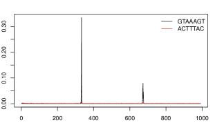
(a)	(b)
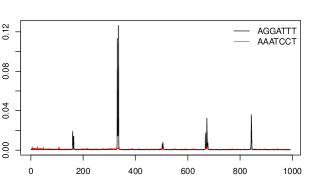
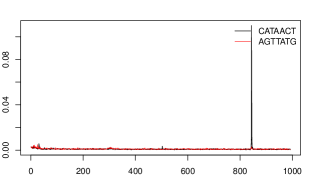
(c)	(d)

Figure 3: Distance distributions of some reverse complements, $f^{w}$ and $f^{\bar{w}}$, with high peak dissimilarity values: (a) $D_{P}=$145.4, $APR$=37.0; (b) $D_{P}=$107.6, $APR$=4.9; (c) $D_{P}=$96.8, $APR$=50.9; (d) $D_{P}=55.75$, $APR$=2.0. Complete genome.

The symmetric pairs with low values of $D_{p}$ have very similar distributions. For some words, this dissimilarity is surprisingly low in spite of their distance distributions having irregular patterns and/or some strong peaks. Some of those distributions, with peak dissimilarities below the $10^{th}$ percentile of $D_{P}$, are illustrated in Fig. 4.

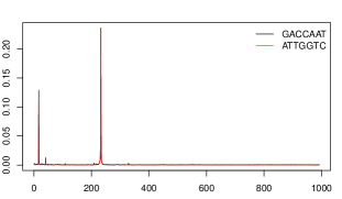
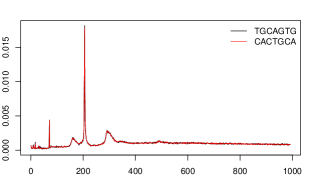
(a)	(b)
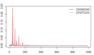
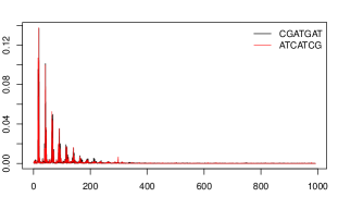
(c)	(d)

Figure 4: Distance distributions of some reverse complements, $f^{w}$ and $f^{\bar{w}}$, with low peak dissimilarity values: (a) $D_{P}$=0.012, $APR$=0.70; (b) $D_{P}$=0.026, $APR$=0.73; (c) $D_{P}$=0.060, $APR$=11.1; (d) $D_{P}$=0.116, $APR$=4.04. Complete genome.

4.2 Combining peak dissimilarity and frequency discrepancy

In order to explore the (dis)similarity between reverse complements we also combine the peak dissimilarity $D_{P}$ with the frequency discrepancy $APR$. Fig. 5 plots $D_{P}$ against $APR$ for each word length, with lines indicating the $90^{th}$ and $99^{th}$ percentile of both. Whereas there is a kind of positive relation between $D_{P}$ and $APR$ for short words, this becomes less clear for longer words, where we know that the rank correlation between these measures decreases (see Table 1).

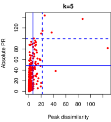
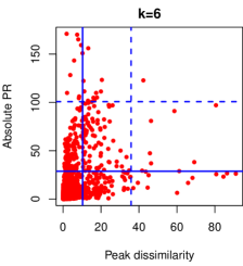
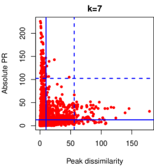
Figure 5: Frequency discrepancy (APR) versus peak dissimilarity, for word lengths 5, 6 and 7. Solid and dashed lines indicate the 90^th and the 99^th percentile of each measure, respectively. Complete genome.

Several combinations of $APR$ and $D_{P}$ are observed in Fig. 5: similar word frequency with similar distance distribution (call this case c1, which is common); dissimilar word frequency with similar distance distribution (c2); and similar word frequency with dissimilar distance distribution (c3). (A fourth combination, dissimilar word frequency and dissimilar distance distribution, becomes increasingly rare for longer words.)

The interesting cases are (c2) and (c3), which may reveal features of interest and should be further studied. In case (c2), words have similar distance distributions but their frequencies of occurrence are quite different, which corresponds to points at the upper left of Fig. 5. To illustrate, consider the symmetric pair with $w=CCGTCCG$ (Fig. 4.c), which has peak dissimilarity below the $10^{th}$ percentile of $D_{P}$ and frequency discrepancy around the $90^{th}$ percentile of $APR$. Conversely, in case (c3) strand symmetry holds but the words have distinct distance distributions along the genome. This corresponds to points at the bottom right of the plot. For instance, the symmetric pair with $w=AGTTATG$ (Fig. 3.d) has peak dissimilarity above the $90^{th}$ percentile of $D_{P}$ and frequency discrepancy around the median of $APR$. Observe that all word pairs listed in Table 3 are located on the right side of the scatter plot.

These results indicate that some asymmetries in the human genome go far beyond Chargaff’s parity rule.

4.3 Deviations from randomness

It is intriguing that the distance distributions of a symmetric pair can be very similar even when their pattern is unexpected. If genomic sequences were generated from independent symbols only subject to Chargaff’s parity rule ($\%A=\%T$ and $\%C=\%G$), the inter-word distance distributions would be close to an exponential distribution. We are interested in investigating how dissimilar distance distributions from such symmetric pairs can be from the pattern under the random scenario. For that purpose, we compute the peak dissimilarity between the averaged distance distribution of the symmetric pair, $(f^{w}+f^{\bar{w}})/2$, and the corresponding averaged reference distribution. The expected distance distribution can be deduced using a state diagram, which represents the progress made towards identifying $w$ as each symbol is read from the sequence. The input parameters are the nucleotide frequencies in the sequence. The algorithm used to construct those reference distributions is a special case of Fu’s procedure based on finite Markov chain embedding [10].

We select all symmetric pairs with intra-pair peak dissimilarity below the $10^{th}$ percentile of $D_{P}$, and ranked them according to the peak dissimilarity between their average distribution and their average reference distribution (denoted as $rs$). This yields a list of symmetric pairs with similar but unexpected distance distributions. For each word length the top 20 results are listed in Table  4. To illustrate some distance distribution of symmetric word pairs with this behaviour, consider the pairs associated with the words $w=CCGTCCG$ [Fig. 4(c)] and $w=ATCATCG$ [Fig. 4(d)], which are listed in this table under $k=7$. The symmetric pairs have very similar distance distributions and their strong peaks make them very dissimilar from the expected distributions in the random scenario.

Table 4: Symmetric pairs with intra-pair peak dissimilarity below the $10^{th}$ percentile of $D_{P}$, sorted by decreasing dissimilarity to the random scenario (only the first 20 results are shown) and organized by word length. For each word $w$ its $D_{P}(w,\bar{w})$ value is given and dissimilarity to the random scenario ($rs$). Complete genome.

k=5			k=6			k=7
$w$	$D_{P}$	$rs$	$w$	$D_{P}$	$rs$	$w$	$D_{P}$	$rs$
CGCCC	0.009	213.80	CGCCCG	0.029	583.44	ACGCGTA	0.141	1621.58
CCTCC	0.015	207.89	CGGGAG	0.018	443.79	CAACGAG	0.122	1556.41
CGGCC	0.014	206.40	GCCTCC	0.005	418.84	CTCGAGA	0.160	1481.80
CCAGC	0.009	190.02	AGGCCG	0.014	360.64	ATCGCCA	0.082	1350.15
CCTCG	0.025	184.80	CAGACG	0.012	354.04	CGTCTGA	0.130	1292.38
CGCCA	0.014	174.63	CAGGAG	0.012	339.94	ACGCAAA	0.056	1257.21
CCGCC	0.014	153.47	GGTCTA	0.034	332.90	GTTCGGA	0.120	1097.62
CAGGC	0.008	136.91	AGATCG	0.024	326.56	ATCATCG	0.116	1040.96
GCCGA	0.024	136.10	CGAGAC	0.025	291.41	CATCGAA	0.111	1038.82
CCCGG	0.021	133.17	CACGCC	0.038	289.29	TCATCGA	0.143	1031.44
CCACC	0.023	115.13	CCCGTC	0.037	276.62	AGGAGCG	0.099	995.72
CTCCC	0.018	103.37	ACGGGG	0.041	267.93	CAGACGA	0.120	957.98
CCCAG	0.011	95.68	CGTCTC	0.009	266.46	TCCCGGA	0.025	904.82
AGGAG	0.011	88.48	GAGGCA	0.018	265.75	GGATCTA	0.138	893.08
GGCCA	0.014	87.62	CCTCCC	0.015	260.13	CCGGACG	0.099	892.40
CAGGA	0.013	83.81	CTCGGC	0.021	258.12	ACGCTCC	0.096	891.33
CCGAG	0.024	78.98	CCCGGC	0.030	246.31	AGACGCT	0.064	886.83
CCAGG	0.027	74.37	CCGGGC	0.029	242.70	CCGTCCG	0.060	866.16
CTGCC	0.021	66.48	CCCGGA	0.042	242.56	CAGACGG	0.009	855.86
AGTAG	0.005	64.42	CGCCTC	0.034	231.77	CGGGCGC	0.030	840.74

4.4 Masked Genome Assembly

To reduce the effect of repetitive sequences in the original genome assembly, we also analyze a masked version of the genome which excludes major known classes of repeats [14], such as long and short interspersed nuclear elements (LINE and SINE), long terminal repeat elements (LTR), Satellite repeats or Simple repeats (micro-satellites). All distributions and measures in this subsection are from the masked sequence and for $k=7$.

Masking the genome sequence markedly affects the shape of the distance distributions. Several strong peaks observed in the complete genome are eliminated by masking, as described in [17]. It also greatly reduces the frequency discrepancy between reverse complements. To visually inspect those discrepancies, we plot the word frequencies against those observed for the reverse complement. We observe that, for the masked genome, the points are located much closer to the diagonal line than in the complete genome [Fig. 6 (a) and (b)].

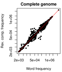
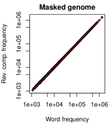
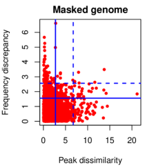
(a)	(b)	(c)

Figure 6: (a) Word frequencies ($n^{w}$) in the entire genome against those observed for the reverse complements ($n^{\bar{w}}$) with both axis in log scale, all for $k=7$; (b) Same for the masked genome; (c) Frequency discrepancy versus peak dissimilarity for $k=7$ in the masked genome, where solid lines indicate the 90^th percentile of each quantity.

To select symmetric pairs with similar and dissimilar distance distributions the authors in [17] retained word pairs with peak dissimilarity below the $10^{th}$ percentile of $D_{P}$ values and those above the $90^{th}$ percentile of $D_{P}$ values, after filtering out words with low total absolute frequency. They distinguish between two groups of word pairs with low peak dissimilarity: those where both distributions have strong peaks at short distances, and on those where neither distribution has strong peaks. These patterns are illustrated in Fig. 7(a–b). Interestingly, the unusual pattern of $w=ATCATCG$ in the complete sequence [Fig. 4(d)] remains in the masked sequence [Fig. 7(b)]. Symmetric pairs with high dissimilarity usually have one distribution with one or more strong peaks at short distances ($<200$) whereas the other presents low variability. Some very dissimilar pairs are shown in Fig. 7(c–d).

(a)	(b)
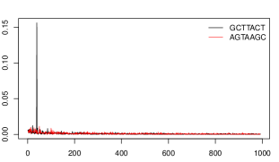
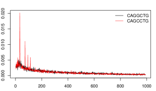
(c)	(d)

Figure 7: Distance distributions of some reverse complements with low dissimilarity values: 0.144 (a), 0.125 (b); and with high dissimilarity values: 11.74 (c), 6.49 (d). Masked genome.

4.4.1 Annotation Analysis

To investigate whether an association exists between dissimilar reverse complements and functional DNA elements, we perform an annotation analysis for the 15 most dissimilar symmetric pairs. For each such pair we list the word with the strongest peaks. Then we look for the ‘favored’ distance(s), i.e. those where the strongest peak(s) are located. These peaks are often concentrated in one chromosome rather than being spread over the entire genome sequence. Table 5 lists the chromosome in which the favored distances are most pronounced, for each of the 15 pairs. The positions of the words occurring at that distance from each other are recorded. Then, we retrieve annotations within these genomic coordinates from UCSC GENCODE v24. Interestingly, the words we obtain that are located on chromosome 13 all fall within the gene LINC01043 (long intergenic non-protein coding RNA 1043) and all of our words on chromosome 1 are contained in the gene TTC34 (tetratricopeptide repeat domain 34). These results suggest that the most dissimilar distributions may be related to repetitive regions associated with RNA or protein structure.

Table 5: The 15 most dissimilar symmetric pairs with $k=7$, characterized by their word with the strongest peaks. The chromosome on which these peaks are prominent is indicated. Masked sequence.

chromosome	13		1	4	3	8
word $w$	$ACCATTC\>$	$GGTAAGC\>$	$AGCATCT\>$	$GTTGGTA\>$	$TGGTATG\>$	$GCTTACT\>$
	$CTTCAGG\>$	$TAAGCAT\>$	$GAGCATC\>$	$TGGTAGA\>$
	$GACCATT\>$	$TCAGGAT\>$	$TGAGCAT\>$
	$TCCTTCA\>$	$TTCAGGA\>$

A deeper investigation into the biological meaning of these words is necessary to investigate whether the observed dissimilarities reflect the selective evolutionary process of the DNA sequence.

5 Conclusions

In this work we explore the DNA symmetry phenomenon in the human genome, by comparing each inter-word distance distribution to the distance distribution of its reverse complement, for word lengths $k=5$, 6 and 7.

We use the peak dissimilarity to evaluate the dissimilarity between the distance distributions of reverse complements and compare it to two well-known measures. Our results suggest that peak dissimilarity achieves its intended purpose in the detection of highly dissimilar distance distributions.

In the complete human genome, we confirm the existence of symmetric word pairs with quite distinct distance distributions. In such cases, one of the distance distributions typically has well defined peaks and the other has low variability. We also report symmetric pairs with very similar distance distributions even though these distributions are themselves unexpected with strong peaks.

The association between distance distribution dissimilarity and frequency discrepancy is analyzed. In general, the correlation between those measures is moderate. Several behaviors are observed in symmetric pairs, by combining low and high values of both measures. In particular there are symmetric pairs that preserve strand symmetry (similar frequency) but have dissimilar distance distributions; and symmetric pairs with dissimilar frequencies and similar distance distributions. Symmetric pairs with either behavior may uncover features of interest.

We also investigate how well our results hold up in a masked sequence, which excludes major known classes of repeats. Even though masking generally reduces the dissimilarity between distance distributions of symmetric pairs, there remain quite a few word pairs with high dissimilarity, which in our study are mainly localized on a specific chromosome and even a specific gene. A question worth investigating is to what extent the high dissimilarities may be linked to evolutionary processes.

Taken together, our results suggest that some asymmetries in the human genome go far beyond Chargaff’s rules. Of particular note are some symmetric pairs with a perfectly ordinary frequency similarity and distribution similarity, that exhibit a strong preference for occurring at some particular distances.

6 acknowledgements

This work was partially supported by the Portuguese Foundation for Science and Technology (FCT), Center for Research & Development in Mathematics and Applications (CIDMA), Institute of Biomedicine (iBiMED) and Institute of Electronics and Telematics Engineering of Aveiro (IEETA), within projects UID/MAT/04106/2013, UID/BIM/04501/2013 and UID/CEC/00127/2013. A. Tavares acknowledges the PhD grant PD/BD/105729/2014 from the FCT. The research of P. Brito was financed by the ERDF - European Regional Development Fund through the Operational Programme for Competitiveness and Internationalization - COMPETE 2020 Programme within project POCI-01-0145-FEDER-006961, and by the FCT as part of project UID/EEA/50014/2013. The research of J. Raymaekers and P. J. Rousseeuw was supported by projects of Internal Funds KU Leuven.

References

- [1] Afreixo, V., Bastos, C.A.C., Garcia, S.P., Rodrigues, J.M.O.S., Pinho, A.J., Ferreira, P.J.S.G.: The breakdown of the word symmetry in the human genome. Journal of Theoretical Biology 335, 153–159 (2013)
- [2] Afreixo, V., Bastos, C.A.C., Pinho, A.J., Garcia, S.P., Ferreira, P.J.S.G.: Genome analysis with inter-nucleotide distances. Bioinformatics 25(23), 3064–3070 (2009)
- [3] Afreixo, V., Rodrigues, J.M.O.S., Bastos, C.A.C.: Analysis of single-strand exceptional word symmetry in the human genome: new measures. Biostatistics 16(2), 209–221 (2015)
- [4] Agresti, A.: An Introduction to Categorical Data Analysis. Wiley Series in Probability and Statistics. Wiley (2007)
- [5] Albrecht-Buehler, G.: Asymptotically increasing compliance of genomes with Chargaff’s second parity rules through inversions and inverted transpositions. Proceedings of the National Academy of Sciences 103(47), 17,828–17,833 (2006)
- [6] Albrecht-Buehler, G.: Inversions and inverted transpositions as the basis for an almost universal ’format’ of genome sequences. Genomics 90(3), 297–305 (2007)
- [7] Baisnée, P.F., Hampson, S., Baldi, P.: Why are complementary DNA strands symmetric? Bioinformatics 18(8), 1021–1033 (2002)
- [8] Benson, G., et al.: Tandem repeats finder: a program to analyze DNA sequences. Nucleic Acids Research 27(2), 573–580 (1999)
- [9] Forsdyke, D.R., Mortimer, J.R.: Chargaff’s legacy. Gene 261(1), 127–137 (2000)
- [10] Fu, J.C.: Distribution theory of runs and patterns associated with a sequence of multi-state trials. Statistica Sinica pp. 957–974 (1996)
- [11] Inagaki, H., Kato, T., Tsutsumi, M., Ouchi, Y., Ohye, T., Kurahashi, H.: Palindrome-mediated translocations in humans: A new mechanistic model for gross chromosomal rearrangements. Frontiers in genetics 7 (2016)
- [12] Jeffreys, H.: An invariant form for the prior probability in estimation problems. In: Proceedings of the Royal Society of London. Series A, Mathematical and Physical Sciences, vol. 186, pp. 453–461. The Royal Society (1946)
- [13] Kullback, S., Leibler, R.A.: On information and sufficiency. The annals of mathematical statistics 22(1), 79–86 (1951)
- [14] Lander, E.S., Linton, L.M., Birren, B., Nusbaum, C., Zody, M.C., Baldwin, J., Devon, K., Dewar, K., Doyle, M., FitzHugh, W., et al.: Initial sequencing and analysis of the human genome. Nature 409(6822), 860–921 (2001)
- [15] Smit, A.F.A., Hubley, R.M., Green, P.: Repeatmasker open–4.0. 2013–2015 (2013). URL http://repeatmasker.org
- [16] Tavares, A.H., Afreixo, V., Rodrigues, J.M.O.S., Bastos, C.A.C.: The symmetry of oligonucleotide distance distributions in the human genome. In: Proceedings of ICPRAM, vol. 2, pp. 256–263 (2015)
- [17] Tavares, A.H., Raymaekers, J., Rousseeuw, P.J., Silva, R.M., Bastos, C.A.C., Pinho, A.J., Brito, P., Afreixo, V.: Dissimilar symmetric word pairs in the human genome. In: 11th International Conference on Practical Applications of Computational Biology & Bioinformatics, pp. 248–256 (2017)
- [18] Zhang, S.H., Huang, Y.Z.: Strand symmetry: Characteristics and origins. In: Bioinformatics and Biomedical Engineering (iCBBE), 2010 4th International Conference on, pp. 1–4. IEEE (2010)