Set-Based Tests for Genetic Association Using the Generalized Berk-Jones Statistic

Abstract

Studying the effects of groups of Single Nucleotide Polymorphisms (SNPs), as in a gene, genetic pathway, or network, can provide novel insight into complex diseases, above that which can be gleaned from studying SNPs individually. Common challenges in set-based genetic association testing include weak effect sizes, correlation between SNPs in a SNP-set, and scarcity of signals, with single-SNP effects often ranging from extremely sparse to moderately sparse in number. Motivated by these challenges, we propose the Generalized Berk-Jones (GBJ) test for the association between a SNP-set and outcome. The GBJ extends the Berk-Jones (BJ) statistic by accounting for correlation among SNPs, and it provides advantages over the Generalized Higher Criticism (GHC) test when signals in a SNP-set are moderately sparse. We also provide an analytic p-value calculation procedure for SNP-sets of any finite size. Using this p-value calculation, we illustrate that the rejection region for GBJ can be described as a compromise of those for BJ and GHC. We develop an omnibus statistic as well, and we show that this omnibus test is robust to the degree of signal sparsity. An additional advantage of our method is the ability to conduct inference using individual SNP summary statistics from a genome-wide association study. We evaluate the finite sample performance of the GBJ though simulation studies and application to gene-level association analysis of breast cancer risk.

Keywords: Correlated tests; Generalized higher criticism; Omnibus test; Sparse alternative; Summary statistics.

1 Introduction

Genome-Wide Association Studies (GWAS) have been successful in identifying the associations between thousands of Single Nucleotide Polymorphisms (SNPs) and a variety of complex traits (Manolio et al., 2009). A traditional GWAS analysis tests for the effect of each individual SNP, and this approach has shown that single-SNP effects are often weak across the genome (Visscher et al., 2012). Recently, set-based tests which jointly analyze a group of SNPs - e.g. SNPs in a gene, pathway, or network - have become increasingly popular as complementary tools which can boost analysis power in GWAS (Wu et al., 2010). These tests are also standard for rare variant analysis in whole genome sequencing studies (Lee et al., 2014).

SNPs can be aggregated into sets based on a variety of genomic features. For example, they can be grouped by physical position, such as location in a gene or Linkage Disequilibrium (LD) block, or similar biological functions, such as membership in a genetic pathway or protein network. Set-based analyses then allow for some natural advantages over individual SNP methods. Besides reducing the number of multiple comparisons across the genome, SNP-set methods can increase power by pooling sparse and weak effects into a stronger aggregated signal, as well as by incorporating biological information into the test (Wu et al., 2011). In addition, set-based interpretations of association may be more meaningful than their single-marker counterparts, such as in a gene-level or pathway-level analysis.

A number of set-based tests for genetic association studies have been developed in recent years, including burden tests (Li and Leal, 2008), the Sequence Kernel Association Test (SKAT) (Wu et al., 2011), the minimum p-value test (MinP) (Conneely and Boehnke, 2007), and most recently the Generalized Higher Criticism (GHC) (Barnett et al., 2017). SKAT and burden tests are examples of methods more suitable for detecting dense signals. If the signals reside in only a few SNPs that are not correlated with noise SNPs, then the power of SKAT and burden tests will suffer.

While certain SNP-sets may contain a large number of signals, it is more common that genomic constructs formed with GWAS data will have only a few signal SNPs. Interestingly, within tests designed for this sparse alternative setting, there are still subtle differences in performance. Under extreme sparsity, as in the case of only one or very few signals in the entire set, the minimum p-value test and the GHC have good power for detecting a SNP-set effect. However GHC and MinP can lose power under moderate sparsity settings, which are relatively common in gene and pathway level analyses of GWAS data. For example, in the Cancer Genetic Markers of Susceptibility (CGEMS) GWAS for breast cancer risk (Hunter et al., 2007), four out of 42 SNPs in the FGFR2 gene, a known breast cancer risk loci, showed strong evidence of association without reaching genome-wide significance. It is hence of substantial interest to develop testing procedures that can reliably detect associations across a range of alternatives in the sparse signal regime.

When factors in a set are independent, several goodness-of-fit type methods have been proposed to perform set-based tests in the presence of sparse signals (Donoho and Jin, 2004; Jager and Wellner, 2007; Walther, 2013). These methods test for the effect of a set by aggregating evidence from marginal test statistics, and they have been shown to possess attractive asymptotic properties when the size of a set goes to infinity. Specifically, they reach a so-called detection boundary when signals are sparse. In a certain sense, they are able to detect the weakest signals detectable by any statistical procedure under the sparse alternative. The class of tests with this ability includes the Higher Criticism (HC) (Donoho and Jin, 2004) and the Berk-Jones (BJ) (Berk and Jones, 1979). Compared to the HC and BJ tests, the minimum p-value test, for example, is known to attain the detection boundary over a smaller portion of the sparse regime. In terms of finite sample performance, it has been demonstrated through simulation that Berk-Jones outperforms Higher Criticism over a range of moderately sparse alternatives when marginal test statistics are independent (Walther, 2013; Li and Siegmund, 2015). Donoho and Jin, (2004) provide an explanation for this result by showing that HC disproportionately weights evidence from the most extreme observed marginal test statistic, at the cost of losing sensitivity to detect signals in other locations.

However, a direct application of BJ to SNP-set testing is not desirable, as standard p-value calculations for BJ rely on independence between elements in a set (Moscovich-Eiger and Nadler, 2017). This assumption is violated by LD-induced correlation between neighboring SNPs in a SNP-set. In addition, we will see that even if we correct the inference procedure of the Berk-Jones, the power of BJ can fall dramatically in high LD settings.

To overcome the challenges posed by correlated SNPs, this paper proposes the Generalized Berk-Jones (GBJ) statistic for testing the association between a SNP-set and outcome. GBJ accounts for LD among SNPs in a set while still preserving the ability to detect moderately sparse and weak signals in finite samples. In fact, GBJ reduces to the Berk-Jones statistic when all SNPs in a set are independent. GBJ can also be applied to SNP-set tests using both individual-level genotype data or GWAS summary statistics from single SNP analysis. To facilitate use, we additionally provide an analytic p-value calculation for GBJ. Our method is more computationally efficient than permutation and is shown to be accurate even at the extremely small levels required for genome-wide significance.

Additional insight into the strengths and weaknesses of GBJ is provided by studying the rejection regions of SNP-set tests developed for sparse alternatives. The rejection regions allow us to quantitatively describe how the power of each test is susceptible to changes in parameters such as the amount of correlation between SNPs or the size of the SNP-set. Since in practice we never have knowledge of the type of alternative, we also propose an omnibus test that combines GBJ, GHC, MinP, and SKAT for added robustness to different degrees of sparsity. An extensive simulation study demonstrates that GBJ outperforms alternative methods in testing SNP-set effects when signals are weak and moderately sparse, and we also show that the omnibus test is robust to a wide range of sparsity levels.

The remainder of the paper is organized as follows. Section 2 discusses the SNP-set testing framework using both individual-level data and GWAS summary statistics. In Section 3 we propose the Generalized Berk-Jones statistic for testing the association between a SNP-set and outcome. We also provide an analytic p-value calculation for GBJ and develop the omnibus test. Section 4 compares the rejection regions of GBJ and other tests designed for the sparse regime. In Section 5 we demonstrate the finite sample performance of GBJ through simulation. Section 6 presents an analysis of the CGEMS data, and we conclude with a discussion in Section 7.

2 The SNP-Set Testing Framework

2.1 Individual-Level Genotype Data

We begin by describing the SNP-set testing framework using individual-level data on genotype, outcome, and other covariates for $n$ total subjects. Suppose for subject $i$, $i=1,...,n$, we observe the outcome $Y_{i}$, a genotype vector $\mathbf{G}_{i}=(G_{i1},...,G_{id})^{T}$ of $d$ SNPs in a SNP-set, and a vector of $q$ covariates $\mathbf{X}_{i}=(X_{i1},...,X_{iq})^{T}$. Assume that $Y_{i}$ conditional on $(\mathbf{G}_{i},\mathbf{X}_{i})$ follows a distribution in the exponential family (McCullagh and Nelder, 1989) with the density function $f(Y_{i})=\exp\left\{(Y_{i}\theta_{i}-b(\theta_{i}))/a_{i}(\phi)+c(Y_{i},\phi)\right\}$, where $a(\cdot)$, $b(\cdot)$, and $c(\cdot)$, are known functions, $\theta_{i}$ is a canonical parameter, and $\phi$ is a dispersion parameter. Let $\mu_{i}=E(Y_{i}|\mathbf{G}_{i},\mathbf{X}_{i})$ denote the conditional mean of $Y_{i}$ and assume it follows the Generalized Linear Model (GLM)

$$g(\mu_{i})=\mathbf{X}_{i}^{T}\boldsymbol{\alpha}+\mathbf{G}_{i}^{T}\boldsymbol{\beta},$$

where $g(\cdot$) is a differentiable monotone link function. We here only consider canonical link functions for simplicity. In matrix notation, the data take the form $\mathbf{Y}=(Y_{1},...,Y_{n})^{T}$, $\mathbf{G}_{n\times d}=[\begin{array}[]{ccccc}\mathbf{G}_{1},...,\mathbf{G}_{n}\end{array}]^{T}$, and $\mathbf{X}_{n\times q}=[\begin{array}[]{ccccc}\mathbf{X}_{1},...,\mathbf{X}_{n}\end{array}]^{T}.$

The null hypothesis of no association between a SNP-set and outcome, after controlling for covariates, is given by $H_{0}:\boldsymbol{\beta}=\mathbf{0}$. Both the size of the set $d$ and the sparsity of signals can vary greatly between sets, e.g. from gene to gene, and the number of nonzero $\beta_{j}$ is unknown. Our aim is to develop a test suitable for different levels of sparsity while also accounting for the correlation among individual SNP test statistics.

The marginal score statistic for $\beta_{j}$, $j=1,...,d$, is

$$Z_{j}=\frac{\mathbf{G}_{.j}^{T}(\mathbf{Y}-\widehat{\boldsymbol{\mu}}_{0})}{\sqrt{\mathbf{G}_{.j}^{T}\mathbf{P}\mathbf{G}_{.j}}},$$

where $\mathbf{G}_{.j}$ denotes the $j$th column vector of $\mathbf{G}$, $\mathbf{P}=\mathbf{W}-\mathbf{W}\mathbf{X}(\mathbf{X}^{T}\mathbf{W}\mathbf{X})^{-1}\mathbf{X}^{T}\mathbf{W}$ is the projection matrix, $\mathbf{W}=\text{diag}\left\{a_{1}(\widehat{\phi})v(\widehat{\mu}_{01}),...,a_{n}(\widehat{\phi})v(\widehat{\mu}_{0n})\right\}$, $\widehat{\mu}_{0i}=g(\mathbf{X}_{i}^{T}\widehat{\boldsymbol{\alpha}}_{0})$, $\widehat{\boldsymbol{\alpha}}_{0}$ is the MLE of $\boldsymbol{\alpha}$ under the null hypothesis, and $v(\mu_{i})=b^{\prime\prime}(\theta_{i})$ is the variance function.

Under the null, the $d$ marginal score test statistics have an asymptotic multivariate normal distribution

$$\mathbf{Z}=\left(Z_{1},\cdots,Z_{d}\right)^{T}\overset{H_{0}}{\sim}N(\mathbf{0}_{d\times 1},\boldsymbol{\Sigma}_{d\times d}),$$

where $\Sigma_{jj}=1$ for all $j$, and for $j\neq k$ we can estimate

$$\widehat{\Sigma}_{jk}=\frac{\mathbf{G}_{.j}^{T}\mathbf{P}\mathbf{G}_{.k}}{\sqrt{\mathbf{G}_{.j}^{T}\mathbf{P}\mathbf{G}_{.j}}\sqrt{\mathbf{G}_{.k}^{T}\mathbf{P}\mathbf{G}_{.k}}}.$$ (1)

2.2 GWAS Summary Statistics

Many GWAS may not release individual-level data due to logistical challenges or data confidentiality agreements. Instead it is much more likely that a marginal test statistic for association with the outcome is available for each individual SNP (Pasaniuc and Price, 2016). It is hence of great interest to be able to perform SNP-set testing using precomputed $Z_{j}$ from across the genome. To test a set of precomputed $Z_{j}$ with GBJ, we require estimation of their correlation matrix $\boldsymbol{\Sigma}$ using external information.

Assume we have a panel of reference genotypes from $n_{r}$ subjects of the same ethnicity as those used to construct the summary statistics. For example, this could come from the publicly available 1000 Genomes dataset (1000 Genomes Project Consortium, 2015). We estimate $\boldsymbol{\Sigma}$ using equation (1) but replace $\mathbf{G}_{.j}$ and $\mathbf{X}$ with $\mathbf{G}_{.j}^{(r)}$ and $\mathbf{X}^{(r)}$, where $\mathbf{G}_{.j}^{(r)}$ is the $n_{r}\times 1$ genotype vector of SNP $j$ from the reference panel, $\mathbf{X}^{(r)}=\left(\mathbf{1},\mathbf{PC}_{1},...,\mathbf{PC}_{m}\right)$, $\mathbf{PC}_{1},...,\mathbf{PC}_{m}$ are the first $m$ principal component vectors calculated from the reference panel, and $m$ is the same number of principal components as was used to control for population stratification (Price et al., 2006) in the original GWAS analysis of the data. Additionally for each subject we estimate $v(\widehat{\mu}_{0i})$ by setting $\widehat{\mu}_{0i}$ equal to the sample mean of the outcome. For a normally distributed outcome, this is exact as $v(\cdot)=1$. For a binary outcome, since population stratification is the primary confounder of the SNP-outcome relationship in GWAS, and because $\mu_{i0}$ generally varies slowly with the principal components, this approximation is practically reasonable. Ultimately we are approximating $\mathbf{G}_{.j}^{T}\mathbf{P}\mathbf{G}_{.k}$ in (1) by $\mathbf{G}_{.j}^{(r)T}\mathbf{G}_{.k}^{(r)}-\mathbf{G}_{.j}^{(r)T}\mathbf{X}^{(r)}\{\mathbf{X}^{(r)T}\mathbf{X}^{(r)}\}^{-1}\mathbf{X}^{(r)T}\mathbf{G}_{.k}^{(r)}$ up to a scale parameter, with the scale parameter eventually cancelled out in $\widehat{\Sigma}_{jk}$.

3 The Generalized Berk-Jones Test for SNP-Set Effects

3.1 The Berk-Jones Statistic

We briefly review the Berk-Jones statistic in this section to help introduce the Generalized Berk-Jones statistic in Section 3.2. The BJ statistic is designed to test for $H_{0}:\boldsymbol{\beta}=0$ against the alternative that a nonempty subset of the $\beta_{j}$ are nonzero, assuming the marginal test statistics are independent. Let $\bar{\Phi}(t)=1-\Phi(t)$ denote the survival function of a standard normal random variable and $\Phi^{-1}(t)$ denote its inverse. Let $|Z|_{(j)}$ denote the order statistics of the vector that results from applying the absolute value operator to each element of $\mathbf{Z}$, so that $|Z|_{(1)}$ is the smallest value of $\mathbf{Z}$ in magnitude.

Set $S(t)=\sum_{j=1}^{d}\mathbf{1}\left(|Z_{j}|\geq t\right)$, which is the number of marginal test statistics with a magnitude greater than or equal to some threshold $t$. For a fixed $t\geq 0$, and if $Z_{j}\overset{\text{iid}}{\sim}N(0,1)$ for all $j$, then $S(t)$ has a binomial distribution with size $d$ and mean parameter $\pi=2\bar{\Phi}(t)$. This viewpoint motivates the Berk-Jones statistic for independent observations (Donoho and Jin, 2004) as:

$$BJ_{d} = \max_{t\geq|Z|_{(d/2+1)}}\left[S(t)\log\left\{\frac{S(t)}{2d\bar{\Phi}(t)}\right\}+\left\{d-S(t)\right\}\log\left\{\frac{1-S(t)/d}{1-2\bar{\Phi}(t)}\right\}\right]\mathbf{1}\left\{2\bar{\Phi}(t)<\frac{S(t)}{d}\right\}$$

$$= \max_{1\leq j\leq d/2}\log\left[\frac{\text{Pr}\left\{S(|Z|_{(d-j+1)})=j\bigg{|}E(\mathbf{Z})=\widehat{\mu}_{j,d}\cdot\mathbf{J}_{d}\right\}}{\text{Pr}\left\{S(|Z|_{(d-j+1)})=j\bigg{|}E(\mathbf{Z})=0\cdot\mathbf{J}_{d}\right\}}\right]\mathbf{1}\left\{2\bar{\Phi}\left(|Z|_{(d-j+1)}\right)<\frac{j}{d}\right\}$$

where $\mathbf{J}_{d}^{T}=(1,1,...,1)_{1\times d}$, $\widehat{\mu}_{j,d}>0$ solves the equation

$$j/d=1-\left\{\Phi(|Z|_{(d-j+1)}-\widehat{\mu}_{j,d})-\Phi(-|Z|_{(d-j+1)}-\widehat{\mu}_{j,d})\right\},$$ (3)

and the second line uses the characterization of $S(t)$ as a binomial random variable.

We see that BJ can roughly be explained as the maximum of a one-sided likelihood ratio test on the mean parameter of $S(t)$, performed over the larger half of observed test statistic magnitudes. At $t=|Z|_{(d-j+1)}$ we have $\pi=2\bar{\Phi}\left(|Z|_{(d-j+1)}\right)$ under the binomial likelihood null, and we have $\pi=j/d$ under the binomial likelihood alternative. We say binomial likelihood null and alternative to make clear that we are talking about an interpretation of the Berk-Jones statistic and to distinguish from the actual set-based null and alternative hypotheses being tested.

Note that the Higher Criticism test differs from the Berk-Jones by replacing the likelihood ratio statistic in (3.1) with the Pearson Chi-square statistic $\{S(t)-2d\bar{\Phi}(t)\}^{2}/\{2d\bar{\Phi}(t)(1-2\bar{\Phi}(t)\}$. Let $k$ be the number of causal SNPs in a set. The sparse regime is designated as $k<d^{1/2}$, and we call $d^{1/4}<k<d^{1/2}$ moderately sparse, with $k\leq d^{1/4}$ referred to as extremely sparse. Donoho and Jin, (2004) showed that, when the $Z_{j}$ are all mutually independent, both HC and BJ are able to reach the detection boundary over the entire sparse signal regime as $d\rightarrow\infty$. Walther, (2013) and Li and Siegmund, (2015) showed that the BJ statistic generally has better power than HC when the size of the set $d$ is finite and the signals are moderately sparse.

If $Z_{1},...,Z_{d}$ are correlated, as they will be for test statistics arising from neighboring SNPs in a gene, then $S(t)$ no longer has a binomial distribution under the null. In this case, the standard Berk-Jones statistic no longer has a meaningful interpretation, and we may expect it to lose efficiency. In fact, we will show later that the rejection region of the Berk-Jones has a less desirable shape under various correlation structures, leading to a significant loss in power when the test statistics are not independent. Therefore we are interested in developing a modified BJ statistic that can account for correlation among the marginal test statistics in a set and thus possesses rejection regions which are more robust to arbitrary correlation structures.

3.2 The Generalized Berk-Jones Statistic

We now propose the Generalized Berk-Jones statistic for testing the association between a SNP-set and outcome. Following the spirit of Berk-Jones, GBJ considers a likelihood ratio type statistic on the mean parameter of $S(t)$, but the key difference is GBJ explicitly accounts for the correlation structure of $Z_{1},...,Z_{d}$. More precisely, we define the GBJ statistic as:

$$GBJ_{d} = \max_{1\leq j\leq d/2}\log\left[\frac{\text{Pr}\left\{S\left(|Z|_{(d-j+1)}\right)=j\bigg{|}E(\mathbf{Z})=\widehat{\mu}_{j,d}\cdot\mathbf{J}_{d},\text{cov}(\mathbf{Z})=\boldsymbol{\Sigma}\right\}}{\text{Pr}\left\{S\left(|Z|_{(d-j+1)}\right)=j\bigg{|}E(\mathbf{Z})=0\cdot\mathbf{J}_{d},\text{cov}(\mathbf{Z})=\boldsymbol{\Sigma}\right\}}\right]$$

$$\cdot\mathbf{1}\left\{2\bar{\Phi}\left(|Z|_{(d-j+1)}\right)<\frac{j}{d}\right\}.$$

When the $Z_{j}$ are correlated, $S(t)$ follows either an underdispersed or overdispersed binomial distribution instead of the standard binomial. However finding the exact distribution of $S(t)$ when $\boldsymbol{\Sigma}\neq\mathbf{I}$ is difficult. For a general $\boldsymbol{\Sigma}$, computing $\text{Pr}\left\{S(t)=m\right\}$ requires iterating through $d$ choose $m$ terms and is very time consuming. In special cases, such as when $\boldsymbol{\Sigma}$ has an exchangeable correlation structure with $\boldsymbol{\Sigma}=(1-\rho)\mathbf{I}+\rho\mathbf{1}\mathbf{1}^{T}$, the calculation is much easier. However these scenarios occur rarely, if ever, in practice.

We propose to approximate the full distribution of $S(t)$ using an Extended Beta-Binomial (EBB) distribution (Prentice, 1986). The Extended Beta-Binomial is a reparameterization and extension of the standard Beta-Binomial$(\alpha,\beta)$ distribution with the standard Beta-Binomial being a special case of the EBB. A random variable $V\sim\text{EBB}\left(d,\lambda,\gamma\right)$ has probability mass function

$$\text{Pr}\left(V=v;d,\lambda,\gamma\right)=\left(\begin{array}[]{c}d\\ v\end{array}\right)\prod_{k=0}^{v-1}(\lambda+\gamma k)\prod_{k=0}^{d-v-1}(1-\lambda+\gamma k)\bigg{/}\prod_{k=0}^{d-1}(1+\gamma k),$$ (4)

where we follow the convention $\prod_{k=0}^{a}c_{k}=1$ for $a<0$. The mean of $V$ is given by $E(V)=d\lambda$ and the variance is $\text{Var}(V)=d\lambda(1-\lambda)\left\{1+(d-1)\gamma(1+\gamma)^{-1}\right\}$.

The Extended Beta-Binomial distribution reduces to the Beta-Binomial distribution if we set $\lambda=\alpha(\alpha+\beta)^{-1}$ and $\gamma=(\alpha+\beta)^{-1}$ for $\alpha,\beta>0$. Because the standard Beta-Binomial distribution requires $\alpha,\beta>0$, it cannot accommodate underdispersion and never reduces to the binomial distribution. In contrast, the EBB allows for both overdispersion and underdispersion, and it reduces exactly to the binomial distribution when $\gamma=0$. This mechanism allows our GBJ statistic to reduce to the Berk-Jones when there is no correlation among the observations.

3.3 Calculation of the Generalized Berk-Jones Statistic

We now describe more precisely the mechanics of calculating the GBJ statistic. To begin, check if the condition $\mathbf{1}\left\{2\bar{\Phi}\left(|Z|_{(d-j+1)}\right)<j/d\right\}$ is satisfied at any $j\leq d/2$. If the condition is never satisfied, then the observed value of GBJ is 0 and we do not need to perform any more computation. The following steps should only be taken on indices $j\leq d/2$ where the condition is satisfied.

At each qualifying $j$, we approximate the distribution of $S(|Z|_{(d-j+1)})$ by an Extended Beta-Binomial random variable under both the binomial likelihood null and the binomial likelihood alternative. Denote these two variables by $V_{0}^{(j)}\sim EBB(\lambda_{0}^{(j)},\gamma_{0}^{(j)})$ and $V_{a}^{(j)}\sim EBB(\lambda_{a}^{(j)},\gamma_{a}^{(j)})$. We solve for $(\lambda_{0}^{(j)},\gamma_{0}^{(j)})$ through moment matching equations

$$\lambda_{0}^{(j)} = E_{0}\left\{S(|Z|_{(d-j+1)})\right\}/d,$$

$$\frac{\gamma_{0}^{(j)}}{1+\gamma_{0}^{(j)}} = \frac{\text{Var}_{0}\left\{S(|Z|_{(d-j+1)})\right\}-d\lambda_{0}^{(j)}(1-\lambda_{0}^{(j)})}{d(d-1)\lambda_{0}^{(j)}(1-\lambda_{0}^{(j)})},$$

where $E_{0}$ and $\text{Var}_{0}$ denote the expectation and variance conditional on $\mathbf{Z}\sim MVN(0\cdot\mathbf{J}_{d},\boldsymbol{\Sigma})$. Similarly, we solve for $(\lambda_{a}^{(j)},\gamma_{a}^{(j)})$ using the same equations except with $E_{a}$ and $\text{Var}_{a}$, which are the expectation and variance conditional on $\mathbf{Z}\sim MVN(\widehat{\mu}_{j,d}\cdot\mathbf{J}_{d},\boldsymbol{\Sigma})$.

The first moment matching equation is simple to solve, since clearly $E_{0}\left\{S(|Z|_{(d-j+1)})\right\}=2d\bar{\Phi}(|Z|_{(d-j+1)})$ and $E_{a}\left\{S(|Z|_{(d-j+1)})\right\}=j$. The variance term in the second equation is more difficult. We can use Theorem 1 of Barnett et al., (2017) for $\text{Var}_{0}$. For $\text{Var}_{a}$, we need the following theorem:

Theorem 1.

Let $\mathbf{Z}\sim MVN(\mu\cdot\mathbf{J}_{d},\boldsymbol{\Sigma})$, and take $\mathcal{H}_{i}(t)$ be the probabilists’ Hermite polynomials. Define $\bar{\rho^{r}}=\frac{2}{d(d-1)}\sum_{1\leq k<l\leq d}\left(\rho_{k,l}\right)^{r}$, where $\rho_{k,l}$ is the $(k,l)$ element of $\boldsymbol{\Sigma}$, and let $\rho_{k,k}=1$ for all $k=1,2,..,d$. Then the variance of $S(t)$ is:

$$\text{Var}_{a}\left\{S(t)\right\} = d\lambda(1-\lambda)+d(d-1)\left\{\phi(t-\mu)^{2}\sum_{r=1}^{\infty}\frac{\bar{\rho^{r}}}{r!}H_{r-1}(t-\mu)^{2}\right\}$$

$$+d(d-1)\left\{\phi(-t-\mu)^{2}\sum_{r=1}^{\infty}\frac{\bar{\rho^{r}}}{r!}H_{r-1}(-t-\mu)^{2}\right\}$$

$$-2d(d-1)\left\{\phi(-t-\mu)\phi(t-\mu)\sum_{r=1}^{\infty}\frac{\bar{\rho^{r}}}{r!}H_{r-1}(-t-\mu)H_{r-1}(t-\mu)\right\},$$

$$\lambda = 1-\left\{\Phi(t-\mu)-\Phi(-t-\mu)\right\}.$$

The proof of this theorem is given in the Supplementary Materials. The terms in the infinite sum shrink very quickly, and in practice we see good accuracy using only the first ten.

After matching all four parameters $(\lambda_{0}^{(j)},\gamma_{0}^{(j)},\lambda_{a}^{(j)},\gamma_{a}^{(j)})$, we calculate

$$GBJ_{d}^{(j)}=\log\left\{\frac{\text{Pr}\left(V_{a}^{(j)}=j;d,\lambda_{a}^{(j)},\gamma_{a}^{(j)}\right)}{\text{Pr}\left(V_{0}^{(j)}=j;d,\lambda_{0}^{(j)},\gamma_{0}^{(j)}\right)}\right\}.$$

The maximum value of $GBJ_{d}^{(j)}$ among all qualifying $j$ is then the observed Generalized Berk-Jones statistic.

3.4 Analytic P-value Calculation

Let $G_{d}$ be a general supremum-based global statistic such as the GBJ statistic. Suppose $G_{d}$ is constructed using independent marginal test statistics $Z_{1},...,Z_{d}$. Denote the observed value of this statistic by $g$, where higher values of $g$ indicate more evidence for the alternative. As noted by Moscovich-Eiger and Nadler, (2017), the p-value for $g$ can often be written

$$\text{Pr}\left(G_{d}\geq g\right)=1-\text{Pr}\left\{\forall j=1,2,...,d:|Z|_{(j)}\leq b_{j}\bigg{|}Z_{j}\overset{iid}{\sim}N(0,1)\right\},$$

where $0\leq b_{1}\leq b_{2}\leq...\leq b_{d}$ are ’boundary points’ that come from inversion of the test statistic. The points $b_{1},b_{2},...,b_{d}$ will depend on $g$ and $d$ and will be different for different choices of a global statistic, but for the sake of presentation, we will suppress this dependency in the notation. Moscovich-Eiger and Nadler, (2017) proposed a method that can calculate the p-value of $G_{d}$ very quickly if $Z_{1},...,Z_{d}$ are independent. However when $Z_{1},...,Z_{d}$ are correlated, their techniques for a fast calculation are not applicable.

An exact p-value for GBJ, and for any global test applied to correlated observations, must take into account the covariance structure of $\mathbf{Z}$. The p-value for these tests is then

$$\text{Pr}\left(G_{d}\geq g\right) = 1-\text{Pr}\left\{\forall j=1,2,...,d:|Z|_{(j)}\leq b_{j}\bigg{|}\mathbf{Z}\sim MVN(\mathbf{0},\boldsymbol{\Sigma})\right\},$$ (5)

where $b_{j}$ is understood to additionally depend on $\boldsymbol{\Sigma}$ as well. We are unaware of any computationally feasible expressions to calculate the joint distribution of the order statistics $|Z|_{(1)},...,|Z|_{(d)}$ when $d$ is moderate or large. The Supplementary Materials provides a procedure to compute this probability by partitioning the region into $d!$ separate sections, but the method is very computationally intensive and not feasible for use with $d>10$.

However, an alternative way to write the rejection region of equation (5) is

$$\text{Pr}\left\{\forall j:|Z|_{(j)}\leq b_{j}\bigg{|}\mathbf{Z}\sim MVN(\mathbf{0},\boldsymbol{\Sigma})\right\}=\text{Pr}\left\{\forall j:S(b_{j})\leq(d-j)\bigg{|}\mathbf{Z}\sim MVN(\mathbf{0},\boldsymbol{\Sigma})\right\}.$$ (6)

The right hand side of (6) suggests that the quantity can be calculated recursively. Indeed, define $b_{0}=0$ and $q_{j,a}=\text{Pr}\left\{S(b_{j})=a,\bigcap_{k=1}^{j-1}S(b_{k})\leq d-k\right\}$. The quantity in (6) is just $q_{d,0}$ and can be calculated recursively as

$$q_{j,a} = \sum_{m=a}^{d-j+1}\text{Pr}\left\{S(b_{j})=a,S(b_{j-1})=m,\bigcap_{k=1}^{j-2}S(b_{k})\leq d-k\right\},$$ (7)

$$= \sum_{m=a}^{d-j+1}\text{Pr}\left\{S(b_{j})=a\bigg{|}S(b_{j-1})=m,\bigcap_{k=1}^{j-2}S(b_{k})\leq d-k\right\}q_{j-1,m},$$

$$\approx \sum_{m=a}^{d-j+1}\text{Pr}\left\{S(b_{j})=a\bigg{|}S(b_{j-1})=m\right\}q_{j-1,m},$$

for $j>1$, with $q_{1,a}=\text{Pr}\left\{S(b_{1})=a|S(b_{0})=d\right\}$. We use an EBB approximation for the distribution of $S(b_{j})$ conditional on $S(b_{j-1})=m$, with the equations

$$\lambda_{j} = \frac{\bar{\Phi}(b_{j})}{\bar{\Phi}(b_{j-1})},$$

$$\frac{\gamma_{j}}{1+\gamma_{j}} = \frac{2\sum_{k<l}\left[\frac{\text{Pr}\left(|Z_{k}|,|Z_{l}|\geq b_{j}\right)}{\text{Pr}\left(|Z_{k}|,|Z_{l}|\geq b_{j-1}\right)}-\left\{\frac{\bar{\Phi}(b_{j})}{\bar{\Phi}(b_{j-1})}\right\}^{2}\right]}{d(d-1)\lambda_{j}(1-\lambda_{j})},$$

to match the moments. Finally, set $\text{Pr}\left\{S(b_{j})=a|S(b_{j-1})=m\right\}:=\text{Pr}\left(V_{j}=a\right)$ where $V_{j}\sim EBB(m,\lambda_{j},\gamma_{j})$. Evaluation of $\text{Pr}\left(|Z_{k}|,|Z_{l}|\geq b_{j}\right)$ follows from steps similar to the proof of Theorem 1.

Note that we can generalize the scheme described above to calculate p-values for many different supremum-based global tests by adopting the general approach of Moscovich-Eiger and Nadler, (2017). As long as the test statistic can be inverted to create the bounds $b_{1},...,b_{d}$, we can use equation (7) to calculate its p-value when applied to correlated observations. In particular, we can use this procedure to perform p-value calculations for the HC, GHC, BJ, and GBJ statistics. Both the calculation and the Generalized Berk-Jones test are implemented in the R package GBJ, available on the CRAN repository.

3.5 The Omnibus Test

While we will show that the Generalized Berk-Jones test possesses an attractive finite sample rejection region when signals are moderately sparse, GBJ may also lose power in the presence of very sparse or dense signals. As SNP-set inference involves testing for a composite alternative $H_{1}:\boldsymbol{\beta}\neq 0$, there is no uniformly optimal test for both sparse and dense alternatives. Since signal sparsity varies between genes, the best test will also change from gene to gene, but it is unknown prior to scanning the genome. Thus we propose an omnibus test that offers robust power over a range of different sparsity levels.

The omnibus test is constructed by combining the SKAT, GBJ, GHC, and minimum p-value statistics, which have been described above. The motivation for choosing these four methods is to combine tests that are known to have good power when signals are dense, moderately sparse, very sparse, and the sparsest possible, respectively. The MinP method uses the set’s largest marginal test statistic in magnitude $|Z|_{(d)}$ as a test statistic. When the $Z_{j}$ are independent, Donoho and Jin, (2004) showed that MinP asymptotically reaches the same detection boundary as HC and BJ in the very sparse regime $k\leq d^{1/4}$ but not the moderately sparse regime $d^{1/4}<k<d^{1/2}$. In finite samples, MinP can have better power than the other three tests when there are only one or two causal SNPs. In contrast, SKAT is known to have high power when signals in a SNP-set are dense.

The omnibus test first applies each of the four tests to the same SNP-set, and then it carries forward the smallest p-value from the four tests as a test statistic. Specifically, the omnibus test statistic is defined as:

$$OMNI=\min\left(p_{GBJ},p_{GHC},p_{SKAT},p_{MinP}\right),$$

where $p_{GBJ},p_{GHC},p_{SKAT}$, and $p_{MinP}$ denote the p-values of the four tests applied on the same SNP-set. As these tests are applied to the same data, the four p-values will be correlated.

Calculations of the p-value for OMNI must again account for the correlation between tests. We employ a Gaussian copula approximation for the joint distribution of the inverse-normal transformed p-values:

$$p_{OMNI}=1-\Phi_{M}\left[\left\{\Phi^{-1}(1-OMNI),...,\Phi^{-1}(1-OMNI)\right\}_{4\times 1};\mathbf{R}_{4\times 4}\right],$$

where $\Phi_{M}(\cdot;\mathbf{R})$ denotes the joint cumulative distribution function of a multivariate normal distribution with mean vector zero and correlation matrix $\mathbf{R}$. The correlation matrix $\mathbf{R}$ of the four component test statistics is estimated through parametric bootstrap under the null. For each subject $i$ in the study, we simulate a new outcome based on the null mean $\widehat{\mu}_{0i}$. When individual-level data are not available, we take $\widehat{\mu}_{0i}$ to be the same constant for all subjects as an approximation. Then each of the four tests are applied with the simulated outcome instead of the original one. The original design matrix, or approximated design matrix if working with summary statistics, is used each time. Each of the four p-values is subtracted from 1 and then inverse-normal transformed; under the null hypothesis the four transformed values have marginal normal distributions with mean zero. As we only need to estimate the correlation matrix $\mathbf{R}$, only a small number of parametric bootstrap samples are needed. In practice, this procedure is repeated 100 times, and then we set $\mathbf{R}$ equal to the sample correlations of the inverse-normal transformed statistics. We will see that this omnibus test performs well across a variety of settings.

4 Rejection Region Analysis of Different SNP-Set Tests

We study in this section the finite sample rejection regions for the BJ, GBJ, HC, and GHC tests, and we advocate for viewing these statistics as boundary-defining algorithms. Consider a fixed SNP-set $s$ with size $d=d_{s}$ and correlation structure $\mathbf{\Sigma}=\mathbf{\Sigma}_{s}$, and suppose we wish to conduct inference at level $\alpha=0.01$. Using the p-value calculation from above, we can employ standard root-finding routines to find the observed value $g_{s}$ which would result in a GBJ p-value of 0.01 for a SNP-set with these characteristics. Then inverting $g_{s}$ to find boundary points $b_{1},b_{2},...,b_{d_{s}}$ as in Section 3.4 constructs a rejection region in terms of in terms of $|Z|_{(1)},...,|Z|_{(d_{s})}$. That is, if the observed value of $|Z|_{(j)}$ were larger than $b_{j}$ for any $j=1,2,...,d_{s}$, then the GBJ p-value for this set would be less than $0.01$. Plotting the bounds for various tests using different values of $\alpha$, $d$, and $\boldsymbol{\Sigma}$ shows us exactly what types of signals a given test is well-powered to detect at level $\alpha$. For the same setting, a test with smaller bounds is preferred, as it will provide more finite sample power.

To numerically compare the rejection boundaries, consider a simplified model of SNP-set correlation structure where the set is partitioned into only two sections. Let one section be the independence section, where all SNPs in this portion are completely independent of all other SNPs in the set. Let the other section be the correlated section, where all SNPs in this portion have common pairwise correlation $\rho$ with other SNPs in the section. For our numerical study, $\rho=0.3$ for the correlated section. We investigate SNP-sets of size $d=20$ and $100$, correlated sections which contain 50% and 75% of the SNPs, and tests at size $\alpha=0.01$. These parameters are chosen to represent reasonable boundaries on the correlation structures seen in common GWAS data; Dawson et al., (2002) estimated that the average $r^{2}$ between SNPs separated by 100kb is around 0.1.

The rejection regions for each SNP-set are plotted in Figure 1. At the $j$th coordinate on the x-axis, if the observed $|Z|_{(j)}$ lies above the boundary of a particular test at that coordinate, then we would reject the null for that test at level $\alpha=0.01$. The lines on the graph are added to aid in visualization, but there should be no interpretation of interpolation between the points. It does not make sense to think of the boundary at $|Z|_{(2.5)}$, for example. While standard methods for inference on HC and BJ are invalid in the presence of correlation, valid p-values for these tests can be computed with the same ideas we have introduced for GBJ inference, specifically following equations (5)-(7). Thus we can show that HC and BJ sometimes have much less desirable rejection regions when SNPs in a set are correlated.

Figure 1: Rejection region of Berk-Jones, Generalized Berk-Jones, Higher Criticism, and Generalized Higher Criticism tests, plotted according to the order statistics of the absolute values of the test statistics. If the $j$th smallest test statistic in magnitude is greater than the boundary point for a given test at any point $j$ on the x-axis, then we would reject the null using that test at level $\alpha=0.01$. The difference between BJ and GBJ becomes much more pronounced as both the size of the set and the amount of correlation increase.

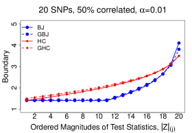
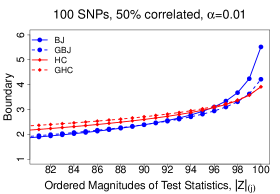
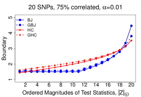
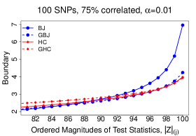
One of the clearest trends from Figure 1 is that the HC and GHC boundaries are lower for a small region around $|Z|_{(d)}$, and then the BJ and GBJ boundaries quickly become smaller as we move left. This behavior indicates that HC and GHC are better at detecting the sparsest alternatives with only a very few signals, as those signals would almost always manifest as the test statistics with the largest magnitude. In contrast, the plots demonstrate that BJ and GBJ can have more power to detect weaker, less sparse signals which may be more easily found by examining the test statistic which is, say, fifth or tenth largest in magnitude. The boundaries of HC and GHC can drop below BJ and GBJ again for the smallest observed magnitudes, but signals would only be found in these observations if they are particularly dense, a setting which is not the focus of our efforts. The intuition we can glean from this figure is closely aligned with the theoretical development of Donoho and Jin, (2004) and the simulations of Li and Siegmund, (2015) when the marginal test statistics $Z_{j}$ are independent. These authors showed that HC is attuned to detect sparse signals arising at the very tail of the observed distribution, while BJ has more power as the number of signals rises.

These results also show why BJ is likely to have low power for detecting sparse signals when the level of correlation is high. When 75% of the SNPs are correlated, the rejection boundary for BJ at the largest few observations is the highest by multiple orders of magnitude on the p-value scale. It would not be desirable to apply BJ in these types of settings, as the test loses an extremely large amount of sensitivity to detect signals in the most outlying values. BJ is still likely to be suitable for detecting dense signals in these situations. Here, GBJ acts as a compromise between BJ and GHC under high correlation. GBJ provides a much lower boundary than BJ at the tail in exchange for slightly higher boundaries near the middle. Thus, GBJ can detect both sparse and dense signals in this example. On the other hand, GBJ provides a slightly higher boundary than GHC at the tail in exchange for lower boundaries past the tail, so it trades some power in the extremely sparse regime for more power to detect moderately sparse signals.

We see that choosing a different statistic is essentially choosing a different boundary-setting algorithm, and this choice should ideally be informed by parameters such as the amount of correlation and estimated sparsity level. Ultimately these plots illustrate that there is no single best global test for all types of alternatives. A genome-wide analysis strategy using the omnibus test will be likely to have robust power across different sparsity settings, correlation structures, and SNP-set sizes.

5 Simulation Results

5.1 Type I Error of the Generalized Berk-Jones Test

We first illustrate that our p-value calculations for the GBJ and omnibus tests are accurate enough to control the Type I error rate at levels required to declare genome-wide significance of a SNP-set. To replicate the setting of traditional GWAS data, we perform the size simulation on random regions across chromosome 5 which correspond to known gene sizes. We also conduct the size simulation on a high-LD subset of the FGFR2 gene and a low-LD subset of the FGFR2 gene to parse LD-related effects. We choose FGFR2 because it contains both high and low LD regions, and because it will later be the most significant gene in our analysis of the CGEMS data. All SNP-sets contain genotypes simulated with HAPGEN2 (Su et al., 2011) using the CEU population from HapMap3 as a reference panel.

In all simulations the outcome is generated as $Y\sim N(0,1)$, and we fit the linear regression model (1) with $\boldsymbol{\beta}=0$ and $\mathbf{X}_{i}=1$. Each simulation is repeated 20 million times, and we report the Type I error down to $10^{-5}$. Table 1 shows that our GBJ p-value calculation is accurate and protects the correct size for correlation structures seen in actual data. The p-value calculation for the omnibus test is similarly accurate at the most stringent significance levels, but it is somewhat conservative at larger significance levels.

Table 1: Type I error of GBJ computed over 20 million simulations. The strong LD setting denoted by SLD refers to eight SNPs from FGFR2 which are highly correlated. The weak LD setting denoted by WLD refers to eight SNPs from FGFR2 which demonstrate only a small amount of correlation with each other. The Chr5 setting refers to over 500 regions on chromosome 5 corresponding to known gene sizes.

Nominal $\alpha$	GBJ, WLD	GBJ, SLD	GBJ, Chr5	OMNI, WLD	OMNI, SLD	OMNI, Chr5
$1\cdot 10^{-2}$	$9.65\cdot 10^{-3}$	$8.50\cdot 10^{-3}$	$9.35\cdot 10^{-3}$	$7.22\cdot 10^{-3}$	$6.88\cdot 10^{-3}$	$6.74\cdot 10^{-3}$
$1\cdot 10^{-3}$	$9.70\cdot 10^{-4}$	$9.21\cdot 10^{-4}$	$1.06\cdot 10^{-3}$	$6.95\cdot 10^{-4}$	$7.19\cdot 10^{-4}$	$6.90\cdot 10^{-4}$
$1\cdot 10^{-4}$	$9.82\cdot 10^{-5}$	$9.90\cdot 10^{-5}$	$1.20\cdot 10^{-4}$	$7.70\cdot 10^{-5}$	$9.00\cdot 10^{-5}$	$8.06\cdot 10^{-5}$
$1\cdot 10^{-5}$	$9.65\cdot 10^{-6}$	$1.11\cdot 10^{-5}$	$1.49\cdot 10^{-5}$	$9.35\cdot 10^{-6}$	$1.31\cdot 10^{-5}$	$1.08\cdot 10^{-5}$

5.2 Power of GBJ Under Varying Hypothetical Correlation Structures and Sparsity Settings

To study the power of GBJ, we first conduct simulations under a variety of hypothetical correlation structures and sparsity settings. The performance of the GBJ is compared to the minimum p-value test, GHC, SKAT, and the omnibus test described in Section 3.5. The MinP test p-value is calculated by casting MinP as a boundary-defining test with $b_{j}=|Z|_{(d)}$ for all $j$, and then computation proceeds through the methods described in Section 3.4. GBJ and GHC similarly use the p-value calculation described above. For SKAT, we run the corresponding R package.

To study how power is impacted by different correlation structures between the SNPs, we utilize block correlation structures which are slightly more complex than those used for the rejection region analysis in Section 4. Specifically, consider a set of causal SNPs that are correlated amongst themselves with common pairwise correlation $\rho_{1}$. All other SNPs are then non-causal, and we allow half of them to have an exchangeable correlation structure with correlation $\rho_{3}$; the other half of the non-causal SNPs are completely independent of all other non-causal SNPs. Finally the pairwise correlation between a causal SNP and a non-causal SNP is set at $\rho_{2}$. The three correlations $\rho_{1},\rho_{2},\rho_{3}$ will vary between 0 and 0.3. All SNPs are generated to have minor allele frequency of 0.3.

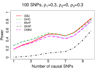
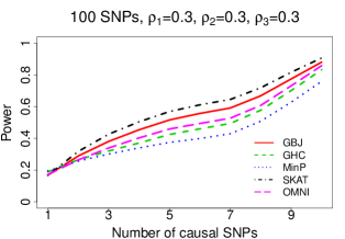
We demonstrate the effects of signal sparsity by using a large SNP-set of $d$=100 SNPs and varying the number of causal SNPs from $k=1$ to $k=10$. This allows us to examine power profiles in the very sparse regime (one to three causal SNPs), in the moderately sparse regime (four to nine causal SNPs), and at the edge of the dense regime (ten or more causal SNPs). The true disease model is

$$Y_{i}=\sum_{j=1}^{k}\beta_{j}G_{ij}+\epsilon_{i},\epsilon_{i}\sim N(0,1),$$ (8)

where all the $\beta_{j}$ are the same and depend on the number of causal SNPs $k$. We reduce $\beta_{j}$ slightly as $k$ increases in order to keep the power of each test below one throughout the entire sparse regime. The full details on effect size for each simulation are available in the Supplementary Materials. Figure 2 considers the case where the noise SNPs are independent, and Figure 3 considers the case where the noise SNPs are correlated. We perform 500 simulations at each different value of $k$ and test at $\alpha=0.01$. All the power curves are smoothed to show empirical power.

Figure 2: Power of set-based tests when noise SNPs are independent. On the left, all SNPs are completely independent of each other. On the right, causal SNPs are correlated within themselves at $\rho_{1}=0.3$. As the number of causal SNPs increases, we slightly decrease the effect size to keep power bounded away from one.

Figure 3: Power of set-based tests when there is correlation within noise SNPs (left) and across all SNPs (right). The correlation structure on the right is slightly simpler than the previous three structures, as we switch to an exchangeable correlation matrix in order to accommodate $\rho_{2}=0.3$ while still ensuring the correlation matrix is positive definite. As the number of causal SNPs increases, we decrease the effect size to keep power bounded away from one.

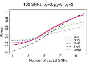
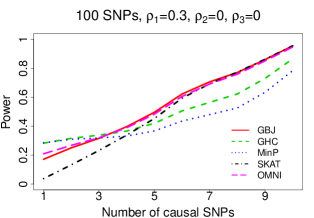
The first significant trend appearing in Figure 2 is the effect of sparsity on power. Among the non-omnibus tests, we see that GHC and MinP perform well when the number of causal SNPs is low, as these tests often have the most power in the very sparse regime. In both panels of Figure 2, the transition to GBJ having more power than GHC and minP occurs in the moderately sparse regime. Then as the number of causal SNPs increases into the dense regime, SKAT begins to catch up and eventually becomes the most powerful test. This behavior matches our intuition as well as previously published simulation results. GHC and minimum p-value place excess weight on the most outlying observations, so they are well-tuned to detect the very sparse signals. The rejection region of GBJ is better-suited to find moderately sparse signals, and SKAT is known to perform well with dense signals.

The relationship between sparsity and power can be modified by the total amount of correlation. In the left panel of Figure 3 we set $\rho_{1}=\rho_{3}=0.3$, which corresponds to the situation where causal SNPs and non-causal SNPs are correlated within themselves, but the two groups are independent of each other. In this case, MinP and GHC become the top-performing tests for a larger range of sparsity settings, with GBJ losing some of its advantage in the moderately sparse regime. SKAT has almost no power in these situations, as the signals are sparse and there is no correlation between causal and non-causal SNPs. It appears that a large amount of correlation between the non-causal SNPs is detrimental to the performance of GBJ. An explanation for this behavior can be found in the rejection region analysis of Figure 1. We see that the bounds of GBJ appear less favorable compared to GHC when the amount of correlation is high. Since over half of the SNPs in Figure 3 are correlated with $\rho_{1}=\rho_{3}=0.3$, these settings represent a much larger amount of total correlation than was present in Figure 2.

In the right panel of Figure 3 we investigate the setting of $\rho_{2}\neq 0$ by using an exchangeable correlation structure, and SKAT dominates as the most powerful test across almost all sparsity levels. Here we break slightly from the above framework by using exchangeable correlation to accommodate $\rho_{2}=0.3$ while still ensuring the correlation matrix of the SNPs is positive definite. GBJ is a close second to SKAT under most sparsity settings with these parameters. SKAT is known to have good performance in the presence of LD between causal SNPs and noise SNPs, which makes signals appear to be dense. The increased density of signals also buoys the performance of GBJ compared to GHC and minimum p-value, which perform the worst under exchangeable correlation.

Never losing too much power compared to the best test, the omnibus test appears to be robust to LD structure and sparsity. This behavior is expected as our omnibus approach integrates information from tests which perform well across multiple sparsity settings. Thus we would anticipate that OMNI is more resilient than any single test.

GBJ also demonstrates good power in a variety of situations, and its overall strength and robustness across the entire sparse regime are attractive properties. In particular, GBJ is the best-performing test when the level of sparsity is moderate and there is weak correlation among the noise SNPs. GBJ is disadvantaged against minP and GHC when signals are extremely sparse or there is excess correlation among noise SNPs, but it outperforms these tests as signals become more dense. In contrast, GBJ provides slightly less power than SKAT as signals reach the dense regime or when there is moderate correlation between causal and non-causal SNPs, but GBJ is also much more robust than SKAT when signals are sparse and not correlated with noise SNPs. Similar to OMNI, GBJ does not fall far behind the best test in any given situation, which suggests that GBJ is a good choice to use when the signal sparsity is unknown. Power for the standard BJ is not plotted in the interest of space, but it behaves like a dense test, similar to SKAT, under correlation. This behavior again matches Figure 1, which showed that BJ is more suited to detect dense signals as the amount of correlation increases.

5.3 Power of GBJ under Actual Chromosome 5 Correlation Structures

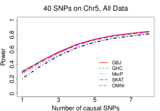
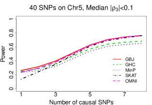
We conduct one final simulation to investigate the power of Generalized Berk-Jones under the unstructured LD patterns found in real GWAS data. In this simulation, we choose blocks of 40 SNPs at random locations on chromosome 5, and then genotype data are generated using HAPGEN2. We choose 40 to again approximately match the characteristics of FGFR2. There are 2000 blocks chosen for each sparsity level, and 10 simulations are performed on each block, for a total of 20000 at each number of causal SNPs. Again, the effect size is decreased as the number of causal SNPs increases, with the outcome still generated from equation (8). Testing is performed at $\alpha=1\cdot 10^{-5}$ to mimic a practical analysis.

We see in the left panel of Figure 4 that GBJ, GHC, and the omnibus test all have very similar power curves in this setting, while SKAT and minP lag slightly behind. As the number of causal SNPs increases, GBJ demonstrates the best power by a small amount. These results are rather homogenous because sparsity levels are more coarse and because the parameters are a mix of the values defined in Figures 2 and 3.

Recall that GBJ extended its advantage over GHC when there was less correlation among noise SNPs. When restricting our analysis to the blocks which have median $|\rho_{3}|<0.1$, we see a more substantial superiority of GBJ over GHC in the moderately sparse regime, similar to Figure 2. Thus it is possible to recover the patterns of the structured simulation in real genotype data. Obviously median $|\rho_{3}|$ is not a perfect summary measure, as it cannot single-handedly capture all the parameters in a $40\times 40$ correlation matrix. Further parsing of the data would be necessary to see larger differences in performance. In a practical setting, we might switch between tests based on certain SNP-set characteristics, such as applying GBJ when the set is large and likely to have moderately sparse signals. These results do again demonstrate the robustness of GBJ across multiple situations, as it provides the most power across a large portion of the sparse regime.

Figure 4: Power of set-based tests with correlation structures found in actual chromosome 5 data. Left panel presents all simulations and right panel shows only SNP-sets where median $|\rho_{3}|<0.1$. The effect size begins at $\beta_{j}=0.16$ and falls to $\beta_{j}=0.1$ so that power remains below one as the number of causal SNPs increases. GBJ is the best-performing test in both panels as the number of causal SNPs increases.

6 Gene-Level Analysis of the CGEMS GWAS Data

The CGEMS breast cancer dataset contains a case-control sample of 1145 breast cancer cases, all postmenopausal women with European ancestry, and 1142 controls recruited from the Nurses’ Health Study. These women were genotyped at approximately 550000 SNPs with the Illumina HumanHap500 array. The dataset was originally analyzed by Hunter et al., (2007) in the single-marker GWAS approach. The authors did not find any individual SNPs to reach the genome-wide significance level of $5\times 10^{-8}$, but they highlighted FGFR2 as a strong candidate for future studies based on four SNPs in the gene that showed suggestive association with breast cancer. Such a situation succinctly illustrates the burden of adjusting for multiple comparisons when testing individual SNPs. Gene-level analysis provides an attractive alternative strategy that can reduce the number of comparisons and also aggregate evidence of signals across multiple SNPs in a gene. Here we perform a gene-level analysis to study the association between genes and breast cancer risk.

Since individual-level genotype data were available for this study, we first calculated the marginal test statistics for each SNP using the model in Section 2.1. Specifically, we fit a logistic regression model with four covariates - age and the first three genotype principal components to control for population structure (Price et al., 2006). Then, for each of 14991 genes, we collected the marginal test statistics for all SNPs located within the region defined by that gene. Each gene with more than one marginal SNP test statistic was analyzed with GBJ, GHC, SKAT, MinP, and the omnibus test.

In Table 2, we rank the top ten genes according to the smallest p-value produced by any of the five tests. In this sample, GBJ provides the strongest evidence of association for the top four genes and five of the top ten. Most of these genes are ranked highly by multiple other methods, however no other method provides the lowest p-value for more than two of the top ten genes. In fact, GHC and MinP produce the smallest p-value only once between the two of them. One possible explanation for the underperformance of GHC and MinP is that there may be multiple tagged SNPs surrounding the true causal loci for each of these genes, which could create a lack of extremely sparse alternatives.

Table 2: Top significant genes in gene-level analysis of CGEMS breast cancer GWAS data, ranked by minimum p-value produced by any of the five tests. The test which produces the smallest p-value for each gene is highlighted in red.

Gene	GHC	GBJ	MinP	SKAT	OMNI	$d$
FGFR2	$2.84\cdot 10^{-5}$	$4.58\cdot 10^{-6}$	$8.20\cdot 10^{-5}$	$3.32\cdot 10^{-5}$	$2.58\cdot 10^{-5}$	$35$
CNGA3	$3.00\cdot 10^{-4}$	$4.04\cdot 10^{-5}$	$1.75\cdot 10^{-3}$	$8.34\cdot 10^{-5}$	$1.84\cdot 10^{-4}$	$26$
PTCD3	$1.21\cdot 10^{-4}$	$5.50\cdot 10^{-5}$	$3.16\cdot 10^{-4}$	$1.87\cdot 10^{-4}$	$6.83\cdot 10^{-5}$	$12$
POLR1A	$9.58\cdot 10^{-5}$	$6.19\cdot 10^{-5}$	$4.62\cdot 10^{-4}$	$4.23\cdot 10^{-4}$	$3.87\cdot 10^{-4}$	$17$
ZNF263	$4.89\cdot 10^{-4}$	$3.90\cdot 10^{-4}$	$8.09\cdot 10^{-4}$	$1.26\cdot 10^{-3}$	$6.84\cdot 10^{-5}$	$3$
VWA3B	$4.20\cdot 10^{-4}$	$2.32\cdot 10^{-4}$	$1.43\cdot 10^{-3}$	$1.48\cdot 10^{-4}$	$4.87\cdot 10^{-4}$	$51$
TBK1	$7.04\cdot 10^{-4}$	$3.35\cdot 10^{-4}$	$1.27\cdot 10^{-3}$	$1.48\cdot 10^{-4}$	$6.05\cdot 10^{-4}$	$11$
ABCA1	$3.74\cdot 10^{-3}$	$1.65\cdot 10^{-4}$	$7.92\cdot 10^{-3}$	$4.99\cdot 10^{-4}$	$2.26\cdot 10^{-4}$	$63$
MMRN1	$2.31\cdot 10^{-4}$	$5.51\cdot 10^{-4}$	$1.72\cdot 10^{-4}$	$3.34\cdot 10^{-2}$	$7.73\cdot 10^{-4}$	$10$
TIGD7	$5.79\cdot 10^{-4}$	$3.78\cdot 10^{-4}$	$1.32\cdot 10^{-3}$	$1.33\cdot 10^{-3}$	$2.05\cdot 10^{-4}$	$4$

The lowest p-value for any gene over all five tests is produced by testing FGFR2 with GBJ, supporting the conclusions of Hunter et al., (2007). Since FGFR2 appears to have signals coming from at least four different SNPs and contains 35 SNPs in total, it would seem to fall into the category of moderate signal sparsity, where GBJ has good performance. Thus we may have expected beforehand that GBJ would be the most powerful test for this gene. FGFR2 has been further validated as a breast cancer associated locus in multiple follow-up studies (Meyer et al., 2008; Liang et al., 2008).

Besides FGFR2, genes such as PTCD3 and POLR1A have also been implicated as risk loci in independent investigations (Boehm et al., 2007; Jia et al., 2011). The overlap of our findings with other studies and other statistics provides a level of reassurance that GBJ performs well in identifying truly significant genes and not simply spurious associations. Alternately, ABCA1 is an example of a gene that may not have received further scrutiny if we were not utilizing the GBJ test. ABCA1 expression has been linked with breast cancer risk (Smith and Land, 2012), but MinP and GHC do not provide the same strength of evidence that GBJ does. It seems likely that there are more than a few signal SNPs in ABCA1, especially since ABCA1 contains a relatively large number of SNPs compared to the other genes in this dataset.

Perhaps due to the limited sample size, no test produces a p-value low enough to be declared significant after Bonferroni correction for 14991 genes. Still, this analysis highlights the advantages of Generalized Berk-Jones compared to alternative tests. The GBJ p-value for FGFR2 does come very close to the Bonferroni-corrected level ($3.34\times 10^{-6}$), and it certainly provides more evidence of association than the single SNP statistics. Additionally, GBJ often gives the highest measure of significance, and never the lowest, in the genes displayed, demonstrating its robustness across different set sizes and LD patterns.

7 Discussion

We have proposed the Generalized Berk-Jones statistic to test for association between a SNP-set and an outcome. Our GBJ generalizes the standard Berk-Jones by modifying the BJ statistic to directly account for the correlation between individual SNPs. This modification results in a test that is more powerful when SNPs are in LD. We also provide an analytic p-value calculation for GBJ and generalize it to a class of supremum-based global tests, allowing valid inference for HC, GHC, BJ, and other methods when these procedures are applied as SNP-set tests using correlated marginal test statistics. Rejection region analysis demonstrates that GBJ can be described as a compromise between Berk-Jones and Higher Criticism-type tests in terms of finite sample performance.

While our numerical analysis shows situations where GBJ does not set the lowest boundary at either $|Z|_{(d)}$ or $|Z|_{(d/2)}$, GBJ generally comes very close to the lowest boundary at both locations, which affords it both robustness to signal sparsity and power to detect moderately sparse signals. GHC and HC often set the lowest boundary around $|Z|_{(d)}$, but in return they concede a large amount of volume past the first few most extreme observations, which lowers power in the moderately sparse regime. BJ frequently sets the lowest boundary past the tail, but its tail boundary can be orders of magnitude larger than that of GBJ, HC, and GHC. Bounds in the expected signal regions must be viewed holistically, so slightly lower bounds at a few locations are not necessarily desirable if the price is much higher bounds in other signal locations, as in the case of BJ. Thus GBJ offers good power to detect moderately sparse effects without losing too much power when single-SNP signals are extremely sparse.

Simulation results reinforce the conclusions we find from examining the rejection regions of GHC and GBJ. Additionally we see that the MinP test performance is quite good when signals are very sparse, similar to GHC, but MinP does not perform as well as GHC when signals become more dense. SKAT has a unique power profile, as it can be particularly powerful when signals are dense or there is correlation between causal and non-causal SNPs, but it is also not robust to different correlation structures and will often have very little power in sparse settings where there is no correlation between causal and non-causal SNPs. The omnibus test offers robust power across different sparsity levels, and while it is rarely the best test, it also never has the worst power. When applied to data from the CGEMS study, we see that GBJ often produces the most significant p-values, perhaps owing to its versatility across different parameter settings.

In demonstrating that the BJ statistic can be adapted for increased robustness to correlation, we have also demonstrated that these types of boundary-defining algorithms can be modified to increase finite sample power under specific set-level parameters. It would be of interest to develop different boundary-defining methods that offer more favorable rejection regions in narrow but well-defined settings. For example, it may be possible to define tests which outperform GHC or minP over finer partitions of the extremely sparse regime.

In a similar vein, it would be interesting to understand the boundary shapes for other previously proposed boundary algorithms (Jager and Wellner, 2007) in the class of Berk-Jones and Higher Criticism. While many of these algorithms share the same asymptotic guarantees of BJ and HC, little is known about their comparative finite sample performance, especially when observations in a set are correlated. These other methods might also have great value in specific settings as mentioned above. It would additionally be very valuable to develop SNP-set tests that are optimal in certain senses for arbitrary sparsity and correlation.

As genomic data collection techniques continue to evolve, it may be necessary to adapt the GBJ as well. In particular, the rise of whole genome sequencing and fine mapping studies is leading to the discovery of more SNPs with extremely rare minor alleles. Marginal test statistics generated from these SNPs are known to be non-Gaussian in finite samples, and thus they will not have the distribution we assume for GBJ. GBJ will need to account for null distributions that are not standard normal before SNP-sets containing rare variants can be tested.

SUPPLEMENTARY MATERIAL

The supplementary materials provide the proof of Theorem 1 from Section 3.3, offer further details on how to calculate the exact p-value from equation (5) in Section 3.4, and list the exact simulation parameters from Section 5.

References

- 1000 Genomes Project Consortium, (2015) 1000 Genomes Project Consortium (2015). A global reference for human genetic variation. Nature, 526(7571):68–74.
- Barnett et al., (2017) Barnett, I., Mukherjee, R., and Lin, X. (2017). The generalized higher criticism for testing SNP-set effects in genetic association studies. Journal of the American Statistical Association, 112(517):64–76.
- Berk and Jones, (1979) Berk, R. H. and Jones, D. H. (1979). Goodness-of-fit test statistics that dominate the kolmogorov statistics. Probability Theory and Related Fields, 47(1):47–59.
- Boehm et al., (2007) Boehm, J. S., Zhao, J. J., Yao, J., Kim, S. Y., Firestein, R., Dunn, I. F., Sjostrom, S. K., Garraway, L., Weremowicz, S., and Richardson, A. (2007). Integrative genomic approaches identify IKBKE as a breast cancer oncogene. Cell, 129:1065.
- Conneely and Boehnke, (2007) Conneely, K. and Boehnke, M. (2007). So many correlated tests, so little time! Rapid adjustment of p-values for multiple correlated tests. The American Journal of Human Genetics, 81:1158.
- Dawson et al., (2002) Dawson, E., Abecasis, G. R., Bumpstead, S., Chen, Y., Hunt, S., Beare, D. M., Pabial, J., Dibling, T., Tinsley, E., Kirby, S., Carter, D., Papaspyridonos, M., Livingstone, S., Ganske, R., Lõhmussaar, E., Zernant, J., Tõonisson, N., Remm, M., Mägi, R., Puurand, T., Vilo, J., Kurg, A., Rice, K., Deloukas, P., Mott, R., Metspalu, A., Bentley, D. R., Cardon, L. R., and Dunham, I. (2002). A first-generation linkage disequilibrium map of human chromosome 22. Nature, 418(6897):544–548.
- Donoho and Jin, (2004) Donoho, D. and Jin, J. (2004). Higher criticism for detecting sparse heterogeneous mixtures. Annals of Statistics, 32(3):962–994.
- Hunter et al., (2007) Hunter, D., Kraft, P., Jacobs, K., Cox, D., Yeager, M., Hankinson, S., Wacholder, S., Wang, Z., Welch, R., Hutchinson, A., and Wang, J. (2007). A genome-wide association study identifies alleles in FGFR2 associated with risk of sporadic postmenopausal breast cancer. Nature Genetics, 39(7):870–874.
- Jager and Wellner, (2007) Jager, L. and Wellner, J. A. (2007). Goodness-of-fit tests via phi-divergences. The Annals of Statistics, 35(5):2018–2053.
- Jia et al., (2011) Jia, P., Zheng, S., Long, J., Zheng, W., and Zhao, Z. (2011). dmGWAS: dense module searching for genome-wide association studies in proteinprotein interaction networks. Bioinformatics, 27(1):95–102.
- Lee et al., (2014) Lee, S., Abecasis, G. R., Boehnke, M., and Lin, X. (2014). Rare-variant association analysis: study designs and statistical tests. The American Journal of Human Genetics, 95(1):5–23.
- Li and Leal, (2008) Li, B. and Leal, S. M. (2008). Methods for detecting associations with rare variants for common diseases: application to analysis of sequence data. The American Journal of Human Genetics, 83:311.
- Li and Siegmund, (2015) Li, J. and Siegmund, D. (2015). Higher criticism: -values and criticism. Annals of Statistics, 43(3):1323–1350.
- Liang et al., (2008) Liang, J., Chen, P., Hu, Z., Zhou, X., Chen, L., Li, M., Wang, Y., Tang, J., Wang, H., and Shen, H. (2008). Genetic variants in fibroblast growth factor receptor 2 (FGFR2) contribute to susceptibility of breast cancer in chinese women. Carcinogenesis, 29(12):2341–2346.
- Manolio et al., (2009) Manolio, T. A., Collins, F. S., Cox, N. J., Goldstein, D. B., Hindorff, L. A., Hunter, D. J., and McCarthy, M. I. (2009). Finding the missing heritability of complex diseases. Nature, 461(7265):747–753.
- McCullagh and Nelder, (1989) McCullagh, P. and Nelder, J. A. (1989). Generalized Linear Models. CRC press.
- Meyer et al., (2008) Meyer, K. B., Maia, A.-T., O’Reilly, M., Teschendorff, A. E., Chin, S.-F., Caldas, C., and Ponder, B. A. (2008). Allele-specific up-regulation of FGFR2 increases susceptibility to breast cancer. PLoS Biology, 1(5):e108.
- Moscovich-Eiger and Nadler, (2017) Moscovich-Eiger, A. and Nadler, B. (2017). Fast calculation of boundary crossing probabilities for poisson processes. Statistics & Probability Letters, 123:177–182.
- Pasaniuc and Price, (2016) Pasaniuc, B. and Price, A. L. (2016). Dissecting the genetics of complex traits using summary association statistics. Nature Genetics Reviews, 18:117–127.
- Prentice, (1986) Prentice, R. L. (1986). Binary regression using an extended beta-binomial distribution, with discussion of correlation induced by covariate measurement errors. Journal of the American Statistical Association, 81(394):321–327.
- Price et al., (2006) Price, A. L., Patterson, N. J., Plenge, R. M., Weinblatt, M. E., Shadick, N. A., and Reich, D. (2006). Principal components analysis corrects for stratification in genome-wide association studies. Nature Genetics, 38(8):904–909.
- Smith and Land, (2012) Smith, B. and Land, H. (2012). Anticancer activity of the cholesterol exporter ABCA1 gene. Cell Reports, 2.3:580–590.
- Su et al., (2011) Su, Z., Marchini, J., and Donnelly, P. (2011). HAPGEN2: simulation of multiple disease snps. Bioinformatics, 27(16):2304–2305.
- Visscher et al., (2012) Visscher, P. M., Brown, M. A., McCarthy, M. I., and Yang, J. (2012). Five years of GWAS discovery. The American Journal of Human Genetics, 90(1):7–24.
- Walther, (2013) Walther, G. (2013). The average likelihood ratio for large-scale multiple testing and detecting sparse mixtures. In From Probability to Statistics and Back: High-Dimensional Models and Processes, volume 9, pages 317–326, Beachwood, OH. IMS.
- Wu et al., (2010) Wu, M. C., Kraft, P., Epstein, M. P., Taylor, D. M., Chanock, S. J., Hunter, D. J., and Lin, X. (2010). Powerful SNP-set analysis for case-control genome-wide association studies. The American Journal of Human Genetics, 86(6):929–942.
- Wu et al., (2011) Wu, M. C., Lee, S., Cai, T., Li, Y., Boehnke, M., and Lin, X. (2011). Rare-variant association testing for sequencing data with the sequence kernel association test. The American Journal of Human Genetics, 89(1):82–93.