Constraining properties of high-density matter in neutron stars with magneto-elastic oscillations

Abstract

We discuss torsional oscillations of highly magnetised neutron stars (magnetars) using two-dimensional, magneto-elastic-hydrodynamical simulations. Our model is able to explain both the low- and high-frequency quasi-periodic oscillations (QPOs) observed in magnetars. The analysis of these oscillations provides constraints on the breakout magnetic-field strength, on the fundamental QPO frequency, and on the frequency of a particularly excited overtone. More importantly, we show how to use this information to generically constraint properties of high-density matter in neutron stars, employing Bayesian analysis. In spite of current uncertainties and computational approximations, our model-dependent Bayesian posterior estimates for SGR 1806-20 yield a magnetic-field strength $\bar{B}\sim 2.1^{+1.3}_{-1.0}\times 10^{15}\,$G and a crust thickness of $\Delta r=1.6^{+0.7}_{-0.6}$ km, which are both in remarkable agreement with observational and theoretical expectations, respectively (1-$\sigma$ error bars are indicated). Our posteriors also favour the presence of a superfluid phase in the core, a relatively low stellar compactness, $M/R<0.19$, indicating a relatively stiff equation of state and/or low mass neutron star, and high shear speeds at the base of the crust, $c_{s}>1.4\times 10^{8}\,$cm/s. Although the procedure laid out here still has large uncertainties, these constraints could become tighter when additional observations become available.

1 Introduction

The quasi-periodic oscillations (QPOs) observed in the X-ray tail of so-called giant flares in magnetars (e.g. Israel et al., 2005; Strohmayer & Watts, 2005; Watts & Strohmayer, 2006; Strohmayer & Watts, 2006) have stimulated theoretical research in neutron star oscillations. QPOs have been interpreted as toroidal shear oscillations of the solid crust by various groups, and approaches to constrain the nuclear equation of state (EoS) of the crust have started (see Duncan, 1998; Messios et al., 2001; Strohmayer & Watts, 2005; Piro, 2005; Sotani et al., 2007; Samuelsson & Andersson, 2007; Steiner & Watts, 2009; Samuelsson & Andersson, 2009; Sotani et al., 2013a; Deibel et al., 2014; Sotani et al., 2016, and references therein). However, since the neutron stars where QPOs are observed have the strongest magnetic fields known, it was realized that the interaction of the crust with the magnetic field leads to a very effective coupling of the two (Levin, 2006, 2007; Glampedakis et al., 2006). Detailed theoretical models of both, Alfvén oscillations (Cerdá-Durán et al., 2009; Sotani et al., 2008; Colaiuda et al., 2009) and coupled magneto-elastic oscillations(Gabler et al., 2011, 2012; Colaiuda & Kokkotas, 2011; van Hoven & Levin, 2011, 2012) have been extended to even include the effects of superfluid neutrons which are expected in the neutron star core (van Hoven & Levin, 2011, 2012; Glampedakis et al., 2011; Passamonti & Lander, 2013; Gabler et al., 2013a; Passamonti & Lander, 2014; Gabler et al., 2016).

However, the magneto-elastic model has problems to identify all of the observed QPO frequencies. These can be divided into two groups, each family with frequencies either below or above $260\,$Hz. The low-frequency QPOs confirmed by different groups are: $18$, $26$, $30$, $92$, $150$ (giant flare of SGR 1806-20), and $28$, $53$, $84$, $155$ Hz (giant flare of SGR 1900+14) (see e.g. Israel et al., 2005; Strohmayer & Watts, 2005; Watts & Strohmayer, 2006; Strohmayer & Watts, 2006). Other studies found additional possible oscillations at $17$, $21$, $36$, $59$, and $116\,$Hz (giant flare of SGR 1806-20, Hambaryan et al., 2011), $57\,$Hz (less energetic bursts of SGR 1806-20, Huppenkothen et al., 2014c), and $93$, $127$, and $260\,$Hz (less energetic bursts of SGR J1550-5418, Huppenkothen et al., 2014a). The corresponding high-frequency QPOs are $625\,$Hz and $1840\,$Hz, and have been found in the giant flare of SGR 1806-20. The first magneto-elastic models that succeeded in explaining both low- and high-frequency QPOs were presented by Gabler et al. (2013a) and confirmed by Passamonti & Lander (2014).

The identification of the oscillation mechanisms responsible for the observed QPO frequencies would allow to constrain the properties of the high-density matter in the hardly accessible interior of neutron stars. In addition to improving our knowledge of superfluid parameters, crustal composition, and core composition, one could also gain information about the strength of the interior magnetic field as well as about its configuration. Enormous progress has been achieved in characterising pure crustal shear modes depending on the equation of state (EoS) (Steiner & Watts, 2009; Sotani, 2011; Sotani et al., 2012, 2013a, 2013b; Sotani et al., 2016). However, these models completely neglect the presence of the magnetic field and the resulting coupling between the crust and the core. For the more complicated problem of global magneto-elastic oscillations, only very general constraints on the neutron star EoS and/or magnetic-field properties have thus far been obtained (Sotani et al., 2008; Andersson et al., 2009; Colaiuda & Kokkotas, 2011; Gabler et al., 2013a). In this work we take a step forward in this direction and show how a Bayesian analysis of magneto-elastic oscillations of magnetars may help to constrain different properties of high-density matter in neutron stars.

The organisation of this paper is as follows: in Section 2 we present a summary of our theoretical model based on the work by Gabler et al. (2016). In Section 3 we describe three observational predictions of our theoretical model that can be used to constrain properties of neutron star matter. The corresponding constraints are discussed in Section 4. Finally, our conclusions are presented in Section 5.

2 Theoretical framework

We follow Gabler et al. (2016) and solve the general-relativistic magneto-elastic-hydrodynamical equations with our numerical code MCOCOA (see also Cerdá-Durán et al., 2008, 2009; Gabler et al., 2011, 2012, 2013b, for details). We use a spherically symmetric metric in isotropic coordinates that can be derived from the line element

$$ds^{2}=-\alpha^{2}dt^{2}+\Phi^{4}\hat{\gamma}_{ij}dx^{i}dx^{j}\,,$$ (1)

where $\alpha$, $\Phi$, and $\hat{\gamma}_{ij}\equiv{\rm diag}\left(1,r^{2},r^{2}\sin\theta\right)$ are the lapse function, the conformal factor, and the spatial flat 3-metric, respectively. The circumferential radius $R$ is thus related to the coordinate radius $r$ by $R=\Phi^{2}r$. For our simulations we neglect the dynamics of the spacetime (Cowling approximation).

The equations describing torsional magneto-elastic oscillations are a consequence of the conservation of baryon number, energy, momentum, and Maxwell’s equations. We only consider linear perturbations in axisymmetry. In this case, poloidal and toroidal perturbations decouple and the system of equations can be cast as (Gabler et al., 2011, 2012, 2016):

$$\frac{1}{\sqrt{-g}}\left(\frac{\partial\sqrt{\gamma}\mathbf{U}}{\partial t}+\frac{\partial\sqrt{-g}\mathbf{F}^{i}}{\partial x^{i}}\right)=0\,,$$ (2)

where $x^{i}\equiv(r,\theta)$, $g$ is the determinant of the 4-metric, $\gamma$ is the determinant of the 3-metric, and the state vector $\bf U$ and the flux vectors $\bf F^{i}$ are given by:

$$\mathbf{U} = [S^{(c)}_{\varphi},B^{\varphi}]\,,$$ (3)

$$\mathbf{F}^{r} = \left[-\frac{b_{\varphi}B^{r}}{W^{(c)}}-2\mu_{\mathrm{S}}\Sigma^{r}_{~{}\varphi},-v^{\varphi(c)}B^{r}\right]\,,$$ (4)

$$\mathbf{F}^{\theta} = \left[-\frac{b_{\varphi}B^{\theta}}{W^{(c)}}-2\mu_{\mathrm{S}}\Sigma^{\theta}_{~{}\varphi},-v^{\varphi(c)}B^{\theta}\right]\,.$$ (5)

Here $B^{i}$ is the magnetic field measured by an Eulerian observer while $b_{i}$ is that measured by a co-moving observer, $\Sigma^{\mu\nu}=g^{\mu\mu}\xi^{\nu(c)}_{,\mu}$ is the shear tensor, and $\mathbf{\xi}^{(c)}$ is the displacement ($\xi^{j(c)}_{\,,t}=\alpha v^{j(c)}$). The Lorentz factor $W^{(c)}=\alpha u^{t(c)}$, the three-velocity $v^{i(c)}$, and the generalized momentum density $S^{(c)}_{i}=(\varepsilon_{\star}X_{c}\rho h+b^{2})W^{(c)2}v^{(c)}_{i}-\alpha b_{i}b^{0}$ are those of the charged particles only (protons in this work). Note that superfluid effects are introduced by the mass fraction of charged particles $X_{c}$ and by the entrainment factor $\varepsilon_{\star}=(1-\varepsilon_{n})/(1-\varepsilon_{n}-\varepsilon_{c})$, where $\varepsilon_{n}$ and $\varepsilon_{c}$ are the entrainment coefficients of neutrons and the charged component, respectively. In this work we use the combination of $X_{c}\varepsilon_{\star}$ as a parameter to study possible effects of superfluidity on the oscillations.

To solve the evolution equations we have to provide boundary conditions at the surface of the star. There, the continuous traction condition has to be fulfilled which leads to

$$b^{\varphi}_{\mathrm{crust}} = b^{\varphi}_{\mathrm{atmosphere}}\,,$$ (6)

$$\xi^{\varphi(c)}_{\mathrm{crust,r}} = 0\,.$$ (7)

At the core-crust interface our MHD solver ensures the continuity of the momentum and can cope with the appearing discontinuities. Therefore, we do not apply any additional conditions there. We initiate the simulations with a general perturbation consisting of the overlap of several spherical harmonics, which should excite many of the magneto-elasticoscillations.

Within this effective one-fluid approach we neglect additional effects that arise due to presence of superconducting protons which change the MHD equations, superfluid vortices which may couple to the crust by pinning or which may couple the superfluid neutrons to the charged components by scattering protons off quasi-particles confined in the cores of neutron vortices via the strong (nuclear) force (Sedrakian, 2016). We also neglect any effects arising due to the slow rotation of magnetars. For a detailed discussion we refer the interested reader to Gabler et al. (2016)

The magneto-elastic framework we have just described allows to perform numerical simulations of the evolution of torsional oscillations of perturbed neutron stars. However, the associated space of parameters of the framework is fairly large and its investigation is computationally expensive. The set of parameters include the EoS, the mass of the neutron star, the magnetic field strength and structure, the entrainment parameter ($\varepsilon_{\star}$), the proton fraction ($X_{c}$) and the shear modulus ($\mu_{\rm S}$). Numerical simulations enable to extract the QPO frequencies corresponding to any particular set of parameters. During the last few years the parameter space has been extensively explored and relations between the QPO frequencies and the different parameters have been extracted. In the current work we use the results provided by Sotani et al. (2008); Cerdá-Durán et al. (2009); Gabler et al. (2011, 2012, 2013b, 2013a, 2016). We parameterise the strength of the magnetic field by $\bar{B}$, the equivalent dipole magnetic field (see Gabler et al., 2013b), that corresponds to the magnetic field of a uniformly magnetised sphere rotating rigidly with a radius of $10\,$km and the same dipolar magnetic momentum as our model. This definition allows to compare models with different magnetic-field structure that may have the same dipolar momentum (so their spin-down properties are similar) but a very different surface magnetic-field strength. Moreover, to simplify the analysis, we parameterise the combination $X_{c}\varepsilon_{\star}$ (instead of the individual parameters) to study the effects of superfluidity on the oscillations. This has the advantage to allow us to simulate different conditions without knowing the detailed physical processes that determine the interaction of protons, electrons and neutrons that may or may not be superfluid or superconducting, respectively. Furthermore, using this approach, the different entrainment and interaction processes, like the mutual entrainment, interaction between neutron vortices with normal protons or proton flux tubes, and with the crustal lattice due to pinning, can be estimated.

To complete the exploration of the parameter space performed in previous studies, we also discuss in this work additional simulations. Each of the new models (series N hereafter) has been constructed as a stratified fluid equilibrium configuration using a modified version of the RNS code (Stergioulas & Friedman, 1995), which was extended to solve for dipole magnetic-field structure for passive fields. The dipolar equilibrium magnetic field is then calculated according to the description in Gabler et al. (2013b), closely following the work of Bocquet et al. (1995). As in Gabler et al. (2013b), we define a mean magnetic field strength

$$\bar{B}=\frac{m}{(10{\rm km})^{3}}\left(\frac{10{\rm km}}{R}\right)^{2},$$ (8)

where $m$ is the magnetic dipole moment and $\bar{B}$ is equivalent to the field strength estimate from spin down measurements. For the construction of our stratified equilibrium model we use the EoS of Akmal-Pandharipande-Ravenhall (APR) for the core (Akmal et al., 1998) and of Douchin-Haensel (DH) for the crust (Douchin & Haensel, 2001). Our reference neutron-star model has a mass of $1.4\mathrm{M}_{\odot}$, a radius of $R=12.26\,$km ($r=10.08\,$km) and $\bar{B}\sim 0.56B_{\mathrm{pole}}$ (the mean magnetic field strength is roughly half the dipole magnetic field strength at the pole). Douchin & Haensel (2001) also provide the proton fraction $X_{c}^{0}(r)$. We take the effective masses from Chamel & Haensel (2008) that can be used to calculate the reference entrainment factor $\varepsilon_{\star}^{0}(r)$. Inside the inner crust, neutrons are superfluid but entrained strongly by the Coulomb lattice due to Bragg reflection (Chamel, 2012). As in Gabler et al. (2016) we assume $X_{c}=0.9$ and $\varepsilon_{\star}=1.0$ in the inner crust and $X_{c}=1.0$ and $\varepsilon_{\star}=1.0$ for densities below the neutron drip point where all nucleons are inside the ions of the Coulomb lattice. At the core-crust interface, the solid crust probably transitions into the fluid core through so called pasta phases. Passamonti & Pons (2016) showed that these structures do not effect global magneto-elastic oscillations significantly, and due to yet missing consistent calculation of shear moduli of the pasta phases in the literature, we, thus, neglect the presence of the latter.

3 QPO properties

We start our analysis by collecting information of the QPOs that will be used in Section 4 to constrain the neutron star properties.

3.1 Properties of low-frequency QPOs

We focus on constant-phase (discrete) magneto-elastic QPOS, denoted as ${}^{l}U_{n}$ in Gabler et al. (2016) (where $l$ as the number of maxima inside the crust across magnetic field lines and $n$ is the number of maxima throughout the star along the magnetic field lines in the region where the oscillation dominates). In Gabler et al. (2016) we studied the dependence of the oscillation frequencies of these QPOs on the magnetic-field strength and on $\varepsilon_{\star}X_{c}$. For a fixed value of the shear speed at the base of the crust, $c_{s,{\rm ref}}=1.3744\times 10^{8}$ cm/s, we obtained the following relation for the lowest-order QPO ${}^{2}U_{2}$:

$$f_{{}^{2}U_{2}}[\mathrm{Hz}](c_{s,{\rm ref}}) = 2.8\times(\varepsilon_{\star}X_{c})^{-0.55}$$ (9)

$$+ 0.66\left(\varepsilon_{\star}X_{c}\right)^{-0.33}\bar{B}[10^{14}\mathrm{G}]\,.$$

This expression is a fit to the results of the numerical simulations for values of $\varepsilon_{\star}X_{c}\in[0.046,0.695]$ and ${\bar{B}}\in[7.5,20]\times 10^{14}~{}G$.

To determine the dependence of $f_{{}^{2}U_{2}}$ on the shear speed $c_{s}$ it is not necessary to perform additional simulations. The magneto-elastic equations given in Eq. (2), are invariant under the transformations

$$t^{\prime} = t\,\sqrt{\frac{c_{s}}{c_{s}^{\prime}}}\,,$$ (10)

$$B^{\prime i} = B^{i}\,\sqrt{\frac{c_{s}^{\prime}}{c_{s}}}\,,$$ (11)

$$\xi^{\prime i} = \xi^{i}\,.$$ (12)

Therefore, Eq. (9) can be rescaled accordingly to obtain the dependence on the value of $c_{s}$ as

$$f_{{}^{2}U_{2}}[\mathrm{Hz}] = 2.8\times(\varepsilon_{\star}X_{c})^{-0.55}\sqrt{\frac{c_{s}}{c_{s,{\rm ref}}}}$$ (13)

$$+ 0.66\times(\varepsilon_{\star}X_{c})^{-0.33}\bar{B}[10^{14}\mathrm{G}]\,.$$

This expression has been obtained for a given neutron-star mass and EoS. Any change in mass or radius, either by changing the mass of the star or the EoS, modifies the QPO frequency. Sotani et al. (2008) showed that the frequency of Upper Alfvén QPOs $U_{n}$ satisfies accurate empirical relations that depend on the compactness of the star, $M/R$ (up to ${\mathcal{O}}(M/R)^{2}$). Note that, even when considering the most extreme EoS and masses, the neutron star compactness is limited to $M/R\sim 0.1-0.3$. Within this range, the $U_{n}$ QPO frequency varies by 50$\%$ at most (Sotani et al., 2008). To take into account the dependence of frequency of the constant-phase ${}^{2}U_{2}$ QPOs on compactness, we assume that it follows the same trend as for the Upper Alfvén QPOs $U_{n}$ and apply the correction of Sotani et al. (2008), which leads to

$$f_{{}^{2}U_{2}}(M/R)=2.5f^{\rm ref}_{{}^{2}U_{2}}\left(1-4.58M/R+6.06(M/R)^{2}\right)\,,$$ (14)

where $f^{\rm ref}_{{}^{2}U_{2}}$ is the value given by Eq. (13) and the normalization constant is chosen so as to recover Eq. (13) for the particular compactness of our model ($M/R=0.1723$).

The uncertainty in the estimation of the frequency given by Eq. (14) includes several uncertainties in the derivation of this expression. On the one hand, the error in the fit of the numerical data reported by Gabler et al. (2016) has a relative rms deviation of $9\%$ and an absolute rms deviation of $2.65$ Hz. Additionally, there is an uncertainty of about $4\%$ due to the limited frequency resolution of the Fourier analysis done by Gabler et al. (2016). We can thus estimate the total systematic error in the computation of the frequency of ${}^{2}U_{2}$ as $\sigma_{\rm sys}/f=\sqrt{0.09^{2}+0.04^{2}}\approx 0.1$.

3.2 Breakout and maximum magnetic-field strength

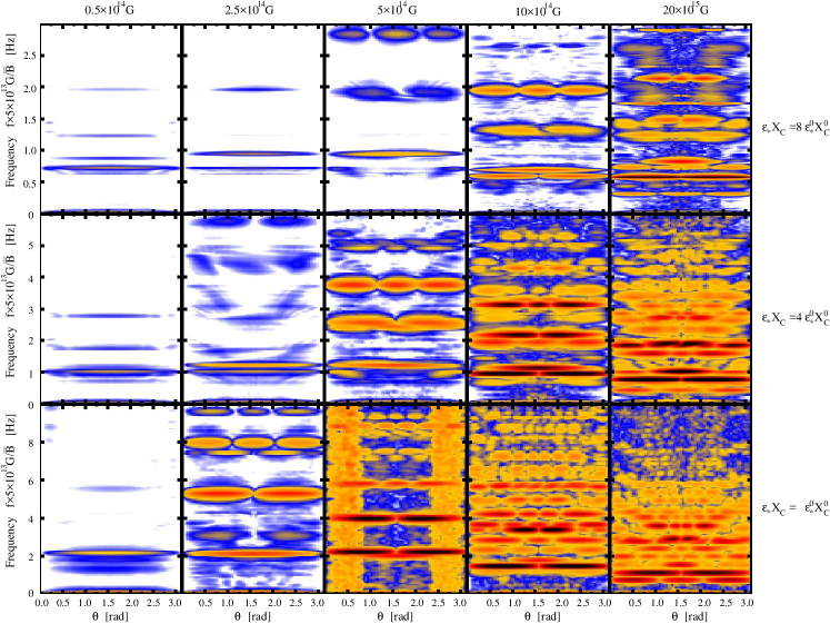
Figure 1: Rescaled Fourier amplitude of the velocity close to the surface as a function of frequency $f$ and polar angle $\theta$ for different combinations of $\bar{B}$ and $\varepsilon_{\star}X_{c}$. The frequency is rescaled by the corresponding magnetic field as $\hat{f}=f\times(5\times 10^{13}\,\mathrm{G}/\bar{B})$. The color scale is logarithmic and ranges from white-blue (minimum) to red-black (maximum)

Depending on the magnetic-field strength, magnetar oscillations may be confined to the core or reach the surface, as shown by Gabler et al. (2012). In that work, we investigated the breakout to the surface of those QPOs which are confined to the core below a certain threshold magnetic-field strength. For a normal fluid core and a dipolar-like magnetic-field configuration, like the one we use here in our new models, the threshold for the breakout is about $\bar{B}\gtrsim 2\times 10^{15}\,$G. We define the breakout to happen when the amplitude of the $FFT$ of ${}^{2}U_{2}$ is larger than that of $L_{2}$, the Lower ocillation which is confined to the closed field lines of the core. For models including superfluid components, the magnetic-field strength threshold also depends on the proton fraction and on the entrainment, $\varepsilon_{\star}X_{c}$.

To study the dependence of the breakout magnetic field on $\varepsilon_{\star}X_{c}$ we perform simulations of our new model series N of our reference neutron star model with different magnetic-field strengths and different values of $\varepsilon_{\star}X_{c}$. We then Fourier analyze the velocity perturbation just below the surface of the neutron star ($r=9.74\,$km, $\rho=1.83\times 10^{8}\,$g$/$cm³) for different polar angles $\theta$. The resolution of the numerical simulations is $150\times 80$ zones for $r\times\theta=[0\,\text{km},10\,\text{km}]\times[0,\pi]$. All models have different Alfvén crossing times and thus the oscillations can have very different frequencies. Since, according to (13), the frequencies depend linearly on $\bar{B}$ and approximately on $\sim 1/\sqrt{\varepsilon_{\star}X_{c}}$ (Gabler et al., 2016), we scale the total simulation time $t$ and the time step $\Delta t$ of each model by $t=t_{0}\times\sqrt{\varepsilon_{\star}X_{c}}/\bar{B}$, in order to directly compare the Fourier amplitude for the different models. We further rescale the obtained Fourier amplitude by the maximum Fourier amplitude of the Lower oscillation $L_{2}$ (see Gabler et al., 2016, for a definition), which should give an independent estimate of the magnitude of the oscillations for a given assumed initial perturbation, because Lower oscillations are not influenced by the interaction with the crust.

In Fig. 1 we plot in a logarithmic colour scale the Fourier amplitude at the surface of the star for a selection of values of $\bar{B}$ and $\varepsilon_{\star}X_{c}$. We rescale the frequencies to $\hat{f}=f\times(5\times 10^{13}\mathrm{G}/\bar{B})$ in order to directly compare the plots for different magnetic-field strengths. The colour scale ranges from white-blue (minimum) to red-black (maximum). Each plot serves as an indicator of whether the oscillations reach the surface (breakout) or remain inside the star. In the former case they could be observed during a magnetar giant flare while in the latter they would not produce any observational signature. In the bottom row for models with $\varepsilon_{\star}X_{c}=\varepsilon_{\star}^{0}X_{c}^{0}$, i.e. in models with superfluid parameters expected from theoretical modelling (Douchin & Haensel, 2001), the Fourier amplitude close to the surface increases rapidly for increasing magnetic-field strength (from left to right) until it saturates at around $\bar{B}\sim 5\times 10^{14}\,$G. At $\bar{B}=5\times 10^{13}\,$G there is almost no Fourier signal, while for $\bar{B}\gtrsim 10^{15}\,$G there are many different oscillations that can be identified by their angular dependence (see also figures 5 and 6 in Gabler et al., 2016). The corresponding frequencies at $\bar{B}=2\times 10^{15}\,$G are given in Table 1 (we identify up to 12 different QPOs - note that their relative amplitudes depend on the ad hoc initial perturbation.).

Oscillation	$f\,$[Hz]	$\hat{f}=f\times(5\times 10^{13}\mathrm{G}/\bar{B})\,$ [Hz]
${}^{3}U_{1}$	$30$	$0.75$
${}^{2}U_{2}$	$44$	$1.10$
${}^{5}U_{1}$	$62$	$1.55$
${}^{4}U_{2}$	$71$	$1.80$
${}^{6}U_{2}$	$80$	$2.00$
${}^{3}U_{3}$	$98$	$2.45$
${}^{5}U_{3}$	$110$	$2.75$
${}^{2}U_{4}$	$115$	$2.88$
${}^{4}U_{4}$	$143$	$3.48$
${}^{6}U_{4}$	$160$	$4.00$
${}^{7}U_{5}$	$172$	$4.30$
${}^{5}U_{5}$	$195$	$4.88$

Table 1: Frequencies $f$ and rescaled frequencies $\hat{f}$ of our fiducial model at $\bar{B}=2\times 10^{15}\,$G and $\varepsilon_{\star}X_{c}=\varepsilon_{\star}^{0}X_{c}^{0}$.

For $\varepsilon_{\star}X_{c}=\varepsilon_{\star}^{0}X_{c}^{0}$ we see that the oscillations reach the surface with the highest amplitudes for the first time for values of $\bar{B}_{\mathrm{breakout}}\in[2.5\times 10^{14}\,$G$,5\times 10^{14}\,$G$]$ (see middle panel of the bottom row in Fig. 1). The maximum amplitude does not increase significantly by further increasing the magnetic-field strength.

The results for two additional values of $\varepsilon_{\star}X_{c}$, namely $8\,\varepsilon_{\star}^{0}X_{c}^{0}$ and $4\,\varepsilon_{\star}^{0}X_{c}^{0}$ are shown in the top and middle row of panels in Fig. 1, respectively. In these models the coupling between the charged components and the neutrons is larger than in the models with $\varepsilon_{\star}X_{c}=\varepsilon_{\star}^{0}X_{c}^{0}$. By increasing $\varepsilon_{\star}X_{c}$ the threshold for the breakout of the oscillations through the crust shifts to higher magnetic-field values. We performed simulations of all possible combinations of $\varepsilon_{\star}X_{c}=\{1,2,4,6,8,10,15,21.7\}\times\varepsilon_{\star}^{0}X_{c}^{0}$ and $\bar{B}=\{0.5,1,2.5,5,7.5,10,15,20\}\times 10^{14}\,$G in order to identify the corresponding value of the breakout magnetic field. Our results are reported in Table 2.

$\varepsilon_{\star}X_{c}/\varepsilon_{\star}^{0}X_{c}^{0}$	1	2	4	6	8	10	15	21.7
$\bar{B}_{\rm breakout}$	3.75	6.25	6.25	8.75	10	15	15	15
[$10^{14}$ G]

Table 2: Breakout magnetic field of the oscillations for different superfluid parameters. The breakout is defined as the point when $|FFT|$ of ${}^{2}U_{2}$ is larger than that of $L_{2}$. When this value is reached between two simulations with different magnetic field strengths we take the mean between the two strengths.

The rescaled frequency of the identified QPOs decreases for $\bar{B}\gtrsim 5\times 10^{14}\,$G in Fig. 1. This decrease is related to the offset in the frequency of the constant-phase QPOs ${}^{l}U_{n}$ due to the interaction with the crust, as discussed in Gabler et al. (2016). Based on the results of Table 2, we find the following dependence of the breakout field on $\varepsilon_{\star}X_{c}$:

$$\bar{B}_{\mathrm{breakout}}=17.23\times 10^{14}\,\mathrm{G}~{}\sqrt{\varepsilon_{\star}X_{c}}\sqrt{\frac{c_{s}}{c_{s,{\rm ref}}}}.$$ (15)

Note that the dependence on $c_{s}$ is obtained using the rescaling of Eqs. (10)-(12), as described in the previous section. The relative rms deviation of this fit with respect to the data in Table 2 is $13\%$ and the relative error in the determination of the $\bar{B}_{\rm breakout}$ itself is $33\%$, due to the limited number of simulations. The systematic error by using this expression is $\sigma_{\rm sys}/\bar{B}_{\mathrm{breakout}}=0.35$ (which should improve significantly if a larger number of simulations in the vicinity of $\bar{B}_{\rm breakout}$ is used). When applying Eq. 15, we implicitely assume that the magnetic field strength does not change significantly through the crust, and thus $\bar{B}_{\mathrm{breakout}}$ is not very sensitve to crust thickness and compactness of the particular stellar model.

While the breakout field represents the minimum field at which QPOs can reach the surface, there is another limitation on the maximum field too, as this must be compatible with the information provided by observations. If the Alfvén velocity inside the crust is much larger than the shear speed there, QPOs disappear and an Alfvén continuum appears (Gabler et al., 2013b; Passamonti & Lander, 2013). This continuum cannot sustain long-lived QPOs and would not explain, in particular, the observations of high-frequency QPOs (Levin, 2006, 2007). Therefore, the maximum magnetic field at the crust, defined as the value at which Alfvén and shear speed are equal, is

$${\bar{B}}_{\mathrm{max}}=1.79\,c_{s}\sqrt{\rho_{\rm cc}}\,,$$ (16)

where the density at the core-crust interface in our model is $\rho_{\rm cc}=1.108\times 10^{14}$ g/cm³, and we have taken into account that the surface field at the pole is $1.79$ times larger than $\bar{B}$, for our reference magnetic-field structure (see Section 2). This maximum field is a rough estimate of the typical magnetic fields at which the transition to an Alfvén-dominated spectrum appears. From Gabler et al. (2013b) we estimate that this transition occurs at magnetic fields deviating no more than $50\%$ of this maximum field. Therefore, the systematic error in the expression for the maximum field is $\sigma_{\rm sys}/{\bar{B}}_{\mathrm{max}}=0.5$.

3.3 High-frequency QPOs

In the preceding sections (and in Gabler et al., 2016) we focused on low-frequency QPOs with frequencies up to $155\,$Hz. These QPOs can be explained with the fundamental magneto-elastic oscillations and some lower overtones. To identify the high-frequency QPOs at $0.625\,$kHz and $1.84\,$kHz with the same kind of oscillations one needs a high overtone of $n\sim 30$ or $90$, respectively. However, to us it seems hard to explain why only these particular overtones should be excited and not many more. A possible explanation was first presented in Gabler et al. (2013b) and was confirmed by Passamonti & Lander (2013). Both groups find a preferential excitation of only a few particular high Alfvén overtones in the core: Let the crust be initially perturbed by a deformation with spatial structure corresponding to the eigenfunction of a crustal shear mode (as may happen during a giant flare). The simulations then show that such an initial perturbation preferentially excites one or a few dominant global magneto-elastic oscillations at different frequencies for dipolar fields $\sim 10^{15}$G, only if the core is assumed to be superfluid. In the latter case the shear terms in the crust are not yet completely dominated by the Alfvén terms.

In the following, we will refer to crustal shear modes of non-magnetized models as pure crustal shear modes and denote them as ${}^{l}t^{(0)}_{n}$ (the index $(0)$ indicating that they are defined in the limit of vanishing magnetic field). Although pure crustal shear modes do not exist for such magnetic field strengths of order $\sim 10^{15}$G, one may regard (in simplified terms) the existence of the preferentially excited global magneto-elastic QPOs as a resonant excitation between a magnetically modified shear oscillation in the crust and a torsional Alfvén oscillation in the core.

Which particular overtones of the magnetically modified shear oscillation are excited depends on the spatial structure of the applied perturbation. To resolve the much finer spatial structures in radial direction of these oscillations we need to increase the resolution of our simulations. Therefore, we have performed simulations of the models of series N with $(300\times 100)$, $(400\times 132)$, and $(500\times 167)$ zones for $r\times\theta=[0\mathrm{km},10\mathrm{km}]\times[0,\pi/2]$. All simulations lead to qualitatively similar results. For the results discussed in this section we assume $\varepsilon_{\star}X_{c}=\varepsilon_{\star}^{0}X_{c}^{0}$.

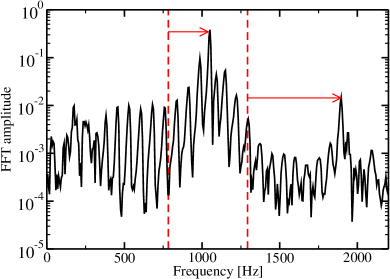
Figure 2: Fourier amplitude of the velocity at one point inside the crust ($r=9.4\,$km, $\theta=0.12$). The initial perturbation uses the eigenfunction of a pure ${}^{2}t^{(0)}_{1}$ crustal shear mode. Dashed red lines indicate the frequencies of the two radial overtones of the pure crustal shear modes, $f_{{}^{2}t^{(0)}_{1}}=0.79\,$kHz and $f_{{}^{2}t_{2}}=1.29\,$kHz. The strongest oscillations during the simulation have significantly higher frequencies $f\sim 1.05\,$kHz and $f\sim 1.9\,$kHz, as indicated by the arrows.

We initiate the simulations with an initial perturbation in the form of the eigenfunction of a ${}^{2}t^{(0)}_{1}$ pure crustal shear mode. Fig. 2 plots, for the highest resolution simulation, the Fourier amplitude at one point inside the crust ($r=9.4\,$km, $\theta=0.12$) for an evolution time of $160\,$ms and $\bar{B}=10^{15}\,$G. There are two local maxima at $f\sim 1.05\,$kHz and $f\sim 1.9\,$kHz, respectively. The global structure and the phase of the Fourier transform of these oscillations are plotted in Fig. 3. These oscillations correspond to the Upper magneto-elastic QPOs ${}^{2}U_{30}$ and ${}^{2}U_{54}$, in the notation of (Gabler et al., 2016). The structure inside the crust along the radial direction is very similar to the ${}^{l}t^{(0)}_{1}$ and ${}^{l}t^{(0)}_{2}$ pure crustal shear modes. We note that there are either one or two radial nodes roughly at the radius where the two pure crustal shear modes have nodes. In the resonance picture, the two excited QPOs could thus be regarded as resonances between two torsional Alfvén Upper QPOs in the core (with $28$ and $50$ maxima in the core region) and magnetically modified crustal shear modes in the crust, which we denote as ${}^{l}t_{1}$ and ${}^{l}t_{2}$, respectively, which result in the global magneto-elastic QPOs ${}^{2}U_{30}$ and ${}^{2}U_{54}$.

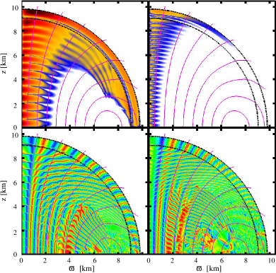
Figure 3: Structure of the Fourier transform and phase of two strongly excited magneto-elastic oscillations ${}^{2}U_{30}$ and ${}^{2}U_{54}$ with $f=1.05\,$kHz (left panels) and $f=1.9\,$kHz (right panels), respectively. Magenta lines indicate the magnetic-field lines and black lines indicate the location of the crust. Top: Fourier amplitude. The colour scale is logarithmic and ranges from white-blue (minimum) to red-black (maximum). Bottom: Phase. The colour scale is linear and ranges from blue ($-\pi/2$) to orange-red ($\pi/2$).

The phase of these oscillations is continuous everywhere, also in the crust, as is shown in Fig. 3. This is in contrast to the constant phase for low-frequency QPOs in superfluid models and could be an artefact of the limited resolution of the simulations and/or a consequence of perturbing the star with a crustal shear mode rather than directly exciting the oscillation itself. We note that when using lower resolution we do not find a constant phase after several mode-recycling steps, i.e. after exciting the star always with the oscillation pattern of the previous simulation at a given frequency. However, it is not surprising that this oscillation has a continuous phase, because the $n\geq 1$ crustal shear modes travel in the radial direction, which coincides with the direction of the magnetic field lines close to the poles. Therefore, the crust hardly couples the field lines together in the perpendicular direction and no constant-phase oscillations form. This is in contrast to the constant-phase oscillations at lower frequencies described in Gabler et al. (2013b, 2016).

Note that, in the Fourier transform of Fig. 2 many more QPOs than just ${}^{2}U_{30}$ and ${}^{2}U_{54}$ are excited. These are all overtones ${}^{2}U_{n}$ with different number $n$ of maxima along the magnetic field lines. However, the ${}^{2}U_{30}$ and ${}^{2}U_{54}$ QPOs form distinct local maxima in the Fourier spectrum. note that ${}^{2}U_{54}$ has a lower amplitude than some QPOs asound ${}^{2}U_{30}$, because the initial excitation in form of $f_{{}^{2}t^{(0)}_{2}}$ preferentially excites QPOs with only one node inside the crust. The red dashed lines in Fig. 2 indicate the frequencies of what would be the pure crustal shear modes $f_{{}^{2}t^{(0)}_{1}}=0.79\,$kHz and $f_{{}^{2}t^{(0)}_{2}}=1.29\,$kHz in a nonmagnetized model, respectively. Clearly, at $f=0.79\,$kHz there is no oscillation, while the $f=1.29\,$kHz frequency happens to (coincidentally) agree with one of the many peaks in the Furier spectrum. Moreover, the spatial structure of the $f=1.29\,$kHz peak has only one node inside the crust in the radial direction and, thus, can not be related directly to ${{}^{2}t^{(0)}_{2}}$.

In view of the above findings, the observed high-frequency QPOs at $0.625$ kHz and $1.84\,$kHz in the giant flare of SGR 1806-20 cannot be interpreted as corresponding to pure crustal shear modes. Instead, they may be due to preferential resonant excitation of particular, global magneto-elastic QPOs, due to the actual seismic event associated with the generation of giant flares. In the following, we will assume that this preferential excitation happens at two different resonant frequencies ${}^{2}U_{n}$ associated with what can be regarded as the two lowest-order magnetically modified crustal shear modes ${}^{2}t_{1}$ and ${}^{2}t_{2}$. Because the order $n$ of the resonantly excited QPOs depend on the EoS, mass and magnetic field, and to simplify the discussion, we will from now on refer to the ${}^{l}t_{1}$ and ${}^{l}t_{2}$ QPOs, meaning, in all cases, the corresponding resonantly excited magnetoelastic, high-frequency ${}^{2}U_{n}$. Our reference to the ${}^{2}t_{1}$ and ${}^{2}t_{2}$ frequencies should thus not be interpreted as meaning pure crustal modes).

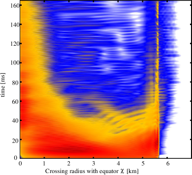
Figure 4: Rescaled kinetic plus magnetic energy along field lines as a function of time for a simulation with $\bar{B}=10^{15}\,$G. Each field line is labeled by its crossing radius with the equatorial plane $\chi$. The closed field line region starts at $\chi\sim 5.5\,$km. The color scale is logarithmic and ranges from white-blue (minimum) to red-black (maximum).

$\bar{B}[10^{14}\,{\rm G}]$		$0.0$	$0.1$	$0.5$	$1.0$	$2.5$	$5.0$	$7.5$	$10$	$20$
$f_{{}^{2}t_{1}}$ [kHz]	$\theta=0$						$0.87$	$0.96$	$1.05$	$1.48$
	$\theta=\pi/4$	$0.80$	$0.77$	$0.77$	$0.78$
	$\theta=\pi/2$					$0.78$	$0.79$	$0.79$	$0.81$	$0.87$
$f_{{}^{2}t_{2}}$ [kHz]	$\theta=0$						($1.51$)	($1.71)$	$(1.85)$	$(>2.0)$
	$\theta=\pi/4$	$1.29$	$1.26$	$1.27$	$1.28$	$1.34$	$(1.46)$
	$\theta=\pi/2$					$1.26$	$(1.29)$	$(1.30)$	$(1.33)$

Table 3: Oscillation frequencies at local maxima of the Fourier amplitude peaks. The values in parenthesis indicate that their determination is not accurate due to the limited resolution of the numerical simulation. The frequencies for $\bar{B}=0.0\,$G are obtained by an eigenmode calculation and may thus differ slightly from those obtained by analyzing the Fourier amplitude of the evolutions. We name the oscillations at $\theta=\pi/2$ as crustal shear modes and the ones at $\theta=0$ ${}^{2}U_{n}$. The latter have different number of maxima $n$ inside the core for different magnetic-field strength $\bar{B}$.

Next, we study the behaviour of the high-frequency QPOs with varying magnetic-field strength. To save computational power and time we use a medium resolution of $400\times 132$. With this grid we obtain the following eigenfrequencies for the pure crustal shear modes ${}^{2}t^{(0)}_{1}$, ${}^{2}t^{(0)}_{2}$ and ${}^{2}t^{(0)}_{3}$ in the absence of a magnetic field: $f_{{}^{2}t^{(0)}_{1}}=0.80\,$Hz, $f_{{}^{2}t^{(0)}_{2}}=1.29\,$kHz and $f_{{}^{2}t^{(0)}_{3}}=1.8\,$kHz, respectively. For non-vanishing magnetic fields, the oscillations of the crust are absorbed rapidly into the core, even at relatively low magnetic field strengths ($\bar{B}\lesssim 2.5\times 10^{14}$G), but there is sufficient time to determine their frequencies. For very weak magnetic fields we expect to recover the frequencies of the eigenmode calculation approximately, and indeed the results of the simulation are off by only a few per cent at $\bar{B}=10^{13}\,$G: $f_{{}^{2}t_{1}}^{\mathrm{}}(10^{13}\text{G})=0.77\,$Hz and $f_{{}^{2}t_{2}}^{\mathrm{}}(10^{13}\text{G})=1.26\,$kHz (see Table 3). For magnetic-field strengths up to $\bar{B}\leq 10^{14}\,G$ the oscillation structure does not change significantly and the frequencies only increase slightly $f_{{}^{2}t_{1}}^{\mathrm{}}(10^{14}\text{G})=0.78\,$Hz and $f_{{}^{2}t_{2}}^{\mathrm{}}(10^{14}\text{G})=1.28\,$kHz. However, the crustal oscillations are damped much faster with increasing magnetic field strength.

For $\bar{B}>10^{14}\,$G the angular oscillation pattern splits into two branches, during the time evolution. One branch stays confined to the crust and its maximum amplitude shifts towards the equator with increasing field strength (see also Figure 4 in Gabler et al., 2013a, for a similar oscillation pattern obtained in the case of a normal fluid core). These localized oscillations are dominated by the shear inside the crust. In the equatorial region the magnetic field is approximately parallel to the $\theta$-direction and, hence, an oscillation that propagates preferentially along the radial direction like the $n\geqslant 1$ crustal shear modes is not prone to interact with the magnetic field. This kind of shear-like oscillations are rapidly damped in regions where the magnetic field has a significant radial component. The frequency of this localized oscillation just outside the region of closed field lines only increase mildly with the magnetic-field strength: e.g. it becomes 0.81 kHz and 1.33 kHz (for oscillations that can be associated with ${}^{2}t^{(0)}_{1}$ and ${}^{2}t^{(0)}_{2}$, respectively at $10^{15}$G. The other branch of oscillations are global magneto-elastic oscillations ${}^{2}U_{n}$ that are concentrated around the polar axis (see Fig. 3). These oscillations appear for $\bar{B}\gtrsim 5\times 10^{14}\,$G and their frequencies increase strongly with increasing magnetic-field strength, e.g. $f_{{}^{2}t_{1}}^{\mathrm{}}(2\times 10^{15}\text{G})=1.48\,$kHz and $f_{{}^{2}t_{2}}^{\mathrm{}}(10^{15}\text{G})=1.85\,$kHz, respectively (see Table 3) .

To illustrate the different time dependence of the two branches we plot in Fig. 4 the rescaled kinetic plus magnetic energy of the oscillations for each magnetic field line as a function of time. The horizontal axis in this plot is the radius $\chi$ at which the magnetic field lines cross the equator (Cerdá-Durán et al., 2008). The open magnetic field lines reach up to $\chi\sim 5.5\,$km. Initially, we apply a perturbation corresponding to the pure crustal shear mode ${}^{2}t^{(0)}_{1}$ and the strongest excitation is seen along the field lines at $\chi\sim 2\,$km. These lines enter the crust at $\theta=\pi/4$ and, as the figure shows, the initial excitation of the crustal shear mode has its maximum amplitude around this angle. After $20\,$ms the energy redistributes and the major part moves to the pole $\chi=0$, while some part moves to the field lines entering the crust close to the equator, $\chi\lesssim 5.5\,$km. At $t>100\,$ms the oscillations near the equator almost completely disappear. Only minimal energy leaks into the region of closed field lines at $\chi\gtrsim 5.5\,$km due to a numerical effect caused by the steep gradients at the core-crust boundary.

The damping time $\tau$ of the localized shear oscillations just outside the region of closed field lines is about $\tau\sim 10\,$ms for the model in Fig. 4 and thus comparable to what was found by van Hoven & Levin (2012). Such a short damping time can not account for the observation of the $625\,$Hz QPO in SGR 1806-20, as its damping time derived from observations is longer than at least about $500\,$ms (Huppenkothen et al., 2014b). On the other hand, the high-frequency magneto-elastic QPO close to the pole survives for much longer times. Its damping time, obtained from the simulation, is limited by the numerical damping of our scheme (see also Gabler et al., 2012). The kinetic plus magnetic energy in all oscillations over the whole neutron star volume decreases at the same rate $\tau\sim 50\,$ms as the energy in the field lines close to pole that mainly represent the excited high-frequency magneto-elastic QPO. Therefore, a damping time of the observations of about $500\,$ms could still be consistent with the simulations for this kind of oscillations.

In Gabler et al. (2016) we showed that the low-frequency, constant-phase oscillations only appear in a certain range of magnetic-field strengths. For the high-frequency oscillations, approximately the same range holds. If the magnetic field is too weak or too strong compared to the shear modulus, shear oscillations in the crust do not resonate with torsional Alfvén oscillations in the core. Moreover, when increasing the superfluid parameter $\varepsilon_{\star}X_{c}$, the range of magnetic-field strengths for observing constant-phase oscillations shrinks. Additionally, this range depends weakly on the particular way the interface between the crust and the core is treated. We have assumed either a discontinuous change or a smooth transition of the shear modulus through the pasta phase. In the discontinuous case the range is narrower. As in Gabler et al. (2013a), our new simulations also show a high-frequency, shear-like oscillation close to the equator in all cases. However, as we already mentioned there, this oscillation has two problems to explain the observed frequencies: firstly, it is transient and rapidly damped, and secondly, it is limited to a region close to the equator where magnetic field lines barely reach the exterior of the star. Being almost confined to the interior these oscillations cannot easily modulate the signal during a giant flare.

To compare with observations, we fit the frequencies of the resonantly excited high-frequency magneto-elastic QPOs given in Table 3 (near the pole), as a function of $\bar{B}_{14}\equiv\bar{B}/10^{14}{\rm G}$

$$f_{{}^{2}t_{n}} \simeq f_{{}^{2}t^{(0)}_{n}}\left(1+a_{2t_{n}}\bar{B}^{2}_{14}\right)^{1/2}\,.$$ (17)

We find $a_{2t_{1}}=0.0063$ and $a_{2t_{2}}=0.012$. Note, however, that the fitting formula (17) is only valid for the particular magnetic-field structure used in our simulations. Irrespective of its structure, the effect of the magnetic field is always to increase the frequency of the magnetically modified crustal oscillation ${}^{2}t_{n}$ above that of the pure crustal mode, ${{}^{2}t^{(0)}_{n}}$:

$$f_{{}^{2}t_{n}}\geq f_{{}^{2}t^{(0)}_{n}}.$$ (18)

Samuelsson & Andersson (2007) estimated that the frequencies of pure crustal modes with $n\geq 1$ assuming constant shear speed inside the crust are proportional to $f_{{}^{2}t^{(0)}_{n}}\sim\left(1-\frac{2M}{R}\right)\frac{2c_{s}}{n\Delta r}$. Comparing to our previous study where we calculated crustal shear mode frequencies (Gabler et al., 2012), we find that the scaling with $M/R$ and $c_{s}$ roughly holds, but the absolute frequency differs significantly because $c_{s}$, which we determine at the core-crust interface, is not equivalent to the mean shear velocity. Thus, we prefer to use the following approximation

$$f_{{}^{2}t^{(0)}_{n}}\simeq\frac{\left(1-\frac{2M}{R}\right)\frac{c_{s}}{\Delta r}}{\left(1-\frac{2M_{\mathrm{ref}}}{R_{\mathrm{ref}}}\right)\frac{c_{s}^{\mathrm{ref}}}{\Delta r_{\mathrm{ref}}}}f^{\mathrm{ref}}_{{}^{2}t^{(0)}_{n}}$$ (19)

where $\Delta r$ indicates the size of the crust and $\mu_{cc}$ is the shear modulus at the core-crust interface. The values of our reference model are $M_{\mathrm{ref}}/R_{\mathrm{ref}}=0.172$ , $\Delta r_{\mathrm{ref}}=870\,$m, $f^{\mathrm{ref}}_{{}^{2}t^{(0)}_{1}}=780\,$Hz, and $f^{\mathrm{ref}}_{{}^{2}t^{(0)}_{2}}=1290\,$Hz. Here, we have neglected the dependence on $l$ ($\lesssim 0.2\%$ correction for $\leqslant 2$). The value of the shear speed in the crust is, however, not constant. We thus contrast the above formula with the calculation of crustal shear modes in Sotani et al. (2007) and find a maximal deviation of $35\%$, which we take as the corresponding systematic error $\sigma_{\rm sys}/f_{{}^{2}t^{(0)}_{n}}=0.35$.

The constraint (18) on the frequency of resonantly excited, high-frequency QPOs depends implicitly on the compactness of the star, because the size of the crust is related to such compactness. Namely, for a given EoS the crust is larger for less compact (less massive) stars. However, since this relation is model dependent, we prefer to follow a more general approach and leave the size of the crust as a free parameter.

So far we have presented a lower bound for the ${}^{2}t_{n}$ frequencies. Additionally, the frequency of these QPOs, cannot become arbitrarily large with increasing magnetic field. The reason is that for sufficiently large magnetic fields, the ${}^{2}t_{n}$ QPOs are dissolved into the Alfvén continuum (see also the corresponding discussion for the low-frequency oscillations in Section 3.2). In our new simulations (see Table 3) the continuum starts to appear at a magnetic field just above $2\times 10^{15}$ G, at which the frequency of the ${}^{2}t_{n}$ QPOs is at most a factor $1.85$ larger than the corresponding pure crustal shear eigenfrequency. Similar results were found by van Hoven & Levin (2012), i.e. an increase of about a factor $2$ in the frequency of the $n\geq 1$ modes at $2\times 10^{15}$ G. Therefore, we introduce the additional constraint

$$f_{{}^{2}t_{n}}<2f_{{}^{2}t^{(0)}_{n}}\,.$$ (20)

To double the frequency of the ${{}^{2}t_{n}}$ QPOs, the magnetic field needs to be so strong, that the Alfvén continuum starts to dominate and no resonant oscillations are allowed.

4 Constraining neutron star properties

4.1 Example model reproducing observed frequencies

In Section 3.1 we discussed the dependency of the frequency of the low-frequency, constant-phase ${}^{2}U_{2}$ mode on the different parameters of the system. Assuming that the magnetic-field strength, the shear speed, and the compactness of the star are known, a clear observational identification of ${}^{2}U_{2}$ would allow us to constrain the parameter $\varepsilon_{\star}X_{c}$. As an example, let us assume that ${}^{2}U_{2}$ is one of the observed QPOs in SGR 1806-20 with the lowest frequencies, $18$, $26$ or $30$ Hz, with $\bar{B}=2\times 10^{15}\,$G. For the given EoS and magnetic-field configuration we thus find $\varepsilon_{\star}X_{c}(r=0)=0.73$, $0.27$ or $0.19$, correspondingly. These values are significantly higher than the value we expect from the EoS, $\varepsilon_{\star}^{0}X^{0}_{c}(r=0)=0.046$, which indicates that, for this model, either the proton fraction has to be higher, or the entrainment should be different, or both.

Similarly, we could constrain the magnetic field strength if we assume that the EoS and related quantities, i.e. $\varepsilon_{\star}^{0}X^{0}_{c}(r=0)=0.046$, are known. In this case, and by using Eq. (14), we obtain a dipolar magnetic-field strength of $\bar{B}\sim 1.1\times 10^{15}\,$G. We performed a new simulation for this case and find that the corresponding spectrum is very similar to that of the previous case. In Fig. 5 we plot the Fourier amplitude at a point near the surface of the star. We identify the 14 strongest frequencies, which are displayed in Table 4. Since this model was fitted to reproduce the oscillation around $30\,$Hz this frequency is recovered. Additionally, we also find significant oscillations near all other higher frequencies ($f<200\,$Hz) that have been reported for SGR 1806-20, i.e. $f\sim 36,59,92,116,150\,$Hz. Naturally, we can only explain one of the lower frequencies $f<30\,$Hz, because we matched the ${}^{2}U_{2}$ mode and only the ${}^{3}U_{1}$ is expected to have a lower frequency. However, the detection of these oscillation frequencies during a giant flare is likely very complicated due to the temporal variation of the flare itself that may produce features in the spectral analysis at these frequencies.

In Fig. 5 we also show the symmetry with respect to the equator of the magnetic-field perturbation for each oscillation. As observed in Gabler et al. (2014a, b) only symmetric (+) oscillations are able to modulate the exterior magnetic field and, hence, the corresponding emission. In the current model, we could thus accommodate the QPOs with $30,92,116,$ and $150\,$Hz, while the oscillations near $36$ and $59\,$Hz should not be observed due to the antisymmetric character of the corresponding magneto-elastic oscillations.

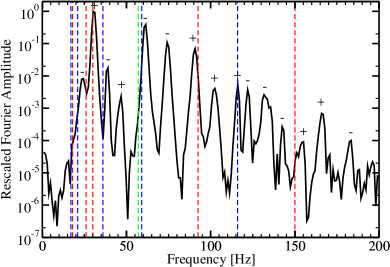
Figure 5: Fourier amplitude at one point inside the crust $r=9.4\,$km and $\theta=0.6$. The dashed red lines indicate the frequencies of the observed QPOs during the giant flare of SGR 1806-20, the blue lines show additional frequencies found by Hambaryan et al. (2011), and the green line shows the frequency found in normal bursts by Huppenkothen et al. (2014c). Plus (minus) signs indicate oscillations that are symmetric (antisymmetric) in $B_{\varphi}$ w.r.t. the equator.

Oscillation	${}^{3}U_{1}$	${}^{2}U_{2}$	${}^{5}U_{1}$	${}^{4}U_{2}$	${}^{3}U_{3}$	${}^{5}U_{3}$	${}^{4}U_{4}$
$f\,$[Hz]	24	30	39	47	61	74	91
Oscillation	${}^{6}U_{4}$	${}^{8}U_{4}$	${}^{5}U_{5}$	${}^{7}U_{5}$	${}^{9}U_{5}$	${}^{6}U_{6}$	${}^{8}U_{6}$
$f\,$[Hz]	102	116	122	132	142	153	169

Table 4: Dominating oscillation frequencies of our fiducial model at $\bar{B}=1.1\times 10^{15}\,$G and $\varepsilon_{\star}X_{c}=\varepsilon_{\star}^{0}X_{c}^{0}$.

Although the magnetic-field configuration in magnetars is currently unknown, the above examples show that it would be possible to constrain properties of the high-density matter of neutron stars through asteroseismology, once some parameters such as the magnetic-field strength, magnetic-field configuration or the mass are constrained by other observations.

…………………………………….

4.2 Combining constraints

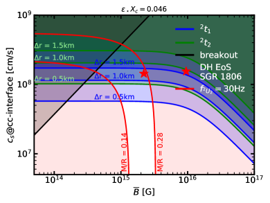
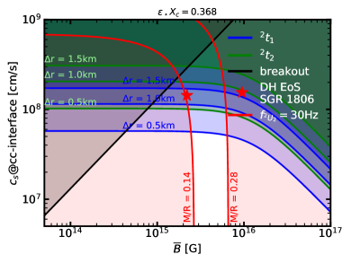
Figure 6: Constraints on the $c_{s}-\bar{B}-$plane obtained from the magneto-elastic QPOs. The frequencies of the resonant high-frequency QPOs have to be below the observed frequencies for ${}^{2}t_{1}$ (blue lines) and ${}^{2}t_{2}$ (green lines). For better visibility we only show the strongest constrain, i.e. for $M/R=0.14$, for the high frequency QPOs. The magnetic field has to be strong enough to break out of the crust. The threshold is given by the black lines. The two red lines indicate the frequency of ${}^{2}U_{2}$ matched to $30\,$Hz for maximum and minimum compactness $M/R$ for typical neutron star models. Shaded areas are excluded from the possible parameter space to explain the observations.

We now combine our previous findings in order to constrain some properties of the magnetar. Plugging Eq. (17) into Eq. (19) we obtain a relation between $\mu_{cc}$ and $\bar{B}$:

$$c_{s}=\sqrt{\frac{\mu_{cc}}{\rho_{cc}}}\lesssim c_{s}^{\mathrm{ref}}\frac{f_{{}^{2}t_{n}}}{f^{\mathrm{ref}}_{{}^{2}t_{n}^{(0)}}}\frac{1}{\sqrt{1+a_{2t_{n}}\bar{B}^{2}}}\frac{\Delta r}{\Delta r_{\mathrm{ref}}}\frac{\left(1-\frac{2M_{\mathrm{ref}}}{R_{\mathrm{ref}}}\right)}{\left(1-\frac{2M}{R}\right)}\,.$$ (21)

The corresponding plots for different crust sizes and for $M/R=0.14$ as the most constraining case are shown in the two panels of Fig. 6 as blue ($n=1$) and green ($n=2$) lines and for $\varepsilon_{\star}X_{c}=0.046$ (left panel) and $\varepsilon_{\star}X_{c}=0.368$ (right panel). Higher shear moduli than those leading to the lines plotted in the figure are excluded, because the oscillation frequency would be too high. The black line in each figure shows the limit of the minimum magnetic field above which the QPO breaks out of the surface, according to Eq. (15). If the shear modulus and therefore $c_{s}$ are too strong, the oscillations stay confined in the core. The last constraint in Fig. 6 is the matching of the low-frequency fundamental oscillation to $f_{{}^{2}U_{2}}=30\,$Hz (Eq. (14)) as indicated with red lines for $M/R=0.14$ and $M/R=0.28$. These values for $M/R$ are chosen because they represent the maximum and minimum compactnesses of typical neutron star models as given in Sotani et al. (2008). All shaded areas in Fig. 6 indicate forbidden regions according to the previous constraints. In addition we also show in the figure the location in the $c_{s}-\bar{B}-$plane of our fiducial model with the DH EoS for the crust with the spin down estimate of the magnetic-field strength of $\bar{B}=2.1\times 10^{15}\,$G for SGR 1806-20.

From Fig. 6 we conclude that for a realistic value of the entrainment factor, $\varepsilon_{\star}X_{c}=0.046$ (left panel), our model with the DH EoS for SGR 1806-20 is consistent with the observations only if the crust is quite extended, $\Delta r\gtrsim 1.3\,$km. If we change the entrainment factor to scan the possible parameter space, we find consistent solutions only up to $\varepsilon_{\star}X_{c}=0.368$ (right panel). For higher values of $\varepsilon_{\star}X_{c}$ the star would be less compact $M/R<0.14$ than allowed by a realistic EoS. In other words, our model constrains the entrainment factor to be $\varepsilon_{\star}X_{c}<0.368$.

4.3 Bayesian analysis

In order to test observational data ${\mathcal{D}}$ against our model ${\mathcal{M}}$, we perform in this section a Bayesian analysis. This analysis allows to describe the state of knowledge about an uncertain hypothesis model ${\mathcal{M}}$ and about the $N$ parameters $\theta_{i}$, $i=1,\dots,N$, of the model. Baye’s theorem,

$$p({\boldsymbol{\theta}}|{\mathcal{D}},{\mathcal{M}})=\frac{p({\mathcal{D}}|{\boldsymbol{\theta}},{\mathcal{M}})\,p({\boldsymbol{\theta}|{\mathcal{M}}})}{p({\mathcal{D}}|{\mathcal{M}})},$$ (22)

allows to compute the posterior probability density function (PDF), $p({\boldsymbol{\theta}}|{\mathcal{D}},{\mathcal{M}})$, for a set of parameters $\boldsymbol{\theta}=\{\theta_{i}\}$, given the model and the data. The likelihood, $p({\mathcal{D}}|{\boldsymbol{\theta}},{\mathcal{M}})$, is the probability to observe certain data, given ${\mathcal{M}}$ and $\boldsymbol{\theta}$, and can be computed straightforwardly from the model, as we see next. The prior PDF of the parameters, $p({\boldsymbol{\theta}|{\mathcal{M}}})$, fulfills

$$\int_{\mathcal{V}}d\theta_{1}\ldots d\theta_{N}\,p({\boldsymbol{\theta}|{\mathcal{M}}})=1\,,$$ (23)

i.e. it is assumed that the parameters of the model only take values in a certain range given by ${\mathcal{V}}$, a $N$-dimensional volume in the parameter space. Finally, the evidence, $p({\mathcal{D}}|{\mathcal{M}})$, is the PDF to observe certain data given a model, regardless of the parameters. It can be computed as

$$p({\mathcal{D}}|{\mathcal{M}})=\int_{\mathcal{V}}d\theta_{1}\ldots d\theta_{N}\,p({\mathcal{D}}|{\boldsymbol{\theta}},{\mathcal{M}})\,p({\boldsymbol{\theta}|{\mathcal{M}}})\,.$$ (24)

The resulting posterior PDF describes the collective knowledge about the different parameters and how they are related. Results for a specific subset of parameters, ${\boldsymbol{\theta}}_{\rm sub}=\{\theta_{a},\theta_{b}...\}$, can be obtain by marginalizing over the rest of the parameters, i.e.

$$p({\boldsymbol{\theta}}_{\rm sub}|{\mathcal{D}},{\mathcal{M}})=\int\prod_{i=1,i\neq a,b,\ldots}^{N}d\theta_{i}\,p({\boldsymbol{\theta}}|{\mathcal{D}},{\mathcal{M}}).$$ (25)

In our model we consider that the observed QPOs are internal oscillations of the magnetar and make the next three model hypothesis:

• ${\mathcal{M}}_{1}$: The QPO frequency observed at about $30$ Hz, corresponds to the frequency of the ${}^{2}U_{2}$ mode given by Eq. (14).

• ${\mathcal{M}}_{2}$: The high-frequency QPO observed at about $600$ Hz, corresponds to the frequency of the magnetically modified ${}^{2}t_{1}$ QPO, and its frequency is larger or equal to that of the corresponding unmagnetized oscillation, given by Eq. (19), and smaller than twice this value (Eq. (20)).

• ${\mathcal{M}}_{3}$: QPOs are only observed if the magnetic field, $\bar{B}$, is higher than the breakout magnetic field given by Eq. (15) and lower than the maximum field given by Eq. (16).

Moreover, this model consists of $N=5$ parameters, namely:

• $\bar{B}$, the magnetar magnetic field. We consider values of $\bar{B}$ in the range $10^{13}$ to $10^{16}$ G, which is a reasonable range for magnetars from observational and theoretical expectations.

• $\varepsilon_{\star}X_{c}$, which is a measure of the coupling between neutrons and protons in the core, and, hence, an indication for superfluidity. Possible values are in the range $0$ to $1$.

• $c_{s}$, the shear speed at the base of the crust. We take values in the range $10^{7}$ to $2\times 10^{8}$ cm/s, which contains all the values considered in Steiner & Watts (2009) (ranging from $3\times 10^{7}$ to $1.4\times 10^{8}$ cm/s).

• $\Delta r$, the crust thickness. We take values in the range $0.3$ to $3$ km, which includes e.g. the range of values in Sotani et al. (2008) from $0.317$ to $1.654$ km.

• $M/R$, the compactness of the star. Typical values for a variety of neutron star masses and EoS give values in the range $0.1$ to $0.3$, which includes e.g. the range of values in Sotani et al. (2008) from $0.14$ to $0.28$.

Given a set of parameters ${\boldsymbol{\theta}}=(\bar{B},\varepsilon_{\star}X_{c},c_{s},\Delta r,M/R)$ it is possible to construct a model ${\mathcal{M}}=({\mathcal{M}}_{1},{\mathcal{M}}_{2},{\mathcal{M}}_{3})$ to compare with observations.

To construct the prior, $p({\boldsymbol{\theta}|{\mathcal{M}}})$, we consider all possible values of $\varepsilon_{\star}X_{c}$, $c_{s}$ and $\Delta r$ equally probable within the parameter space. For the dependence on $\bar{B}$, we construct the prior in order to fulfill model hypothesis ${\mathcal{M}}_{3}$:

$$p({\boldsymbol{\theta}|{\mathcal{M}}}) \propto \frac{1}{2}\left(1+\rm{erf}\left(\frac{\bar{B}-\bar{B}_{\rm breakout}}{\sigma_{\rm sys,breakout}\sqrt{2}}\right)\right)\times$$ (26)

$$\frac{1}{2}\left(1+\rm{erf}\left(\frac{\bar{B}_{\rm max}-\bar{B}}{\sigma_{\rm sys,max}\sqrt{2}}\right)\right),$$

where $\sigma_{\rm sys,breakout}$ and $\sigma_{\rm sys,max}$ correspond to the systematic error estimated in Section 3.2 for $\bar{B}_{\rm breakout}$ and $\bar{B}_{\rm max}$, respectively. The normalization constant is computed in order to fulfill Eq. (23).

For our analysis we consider the RXTE observation of the 2004 giant flare in SGR 1806-20 (Strohmayer & Watts, 2006). We identify the $f_{{}^{2}U_{2}}$ frequency appearing in ${\mathcal{M}}_{1}$ as the QPO at $f^{\rm obs}_{{}^{2}U_{2}}=29.0\pm 0.4$ Hz with a width $\sigma^{\rm obs}_{{}^{2}U_{2}}=4.1$ Hz (data ${\mathcal{D}}_{1}$ hereafter), and the $f_{{}^{2}t_{1}}$ frequency appearing in ${\mathcal{M}}_{2}$ as the QPO at $f^{\rm obs}_{{}^{2}t_{1}}=625.5\pm 0.2$ Hz with a width $\sigma^{\rm obs}_{{}^{2}t_{1}}=1.8$ Hz (data ${\mathcal{D}}_{2}$ hereafter). Using this observational data, ${\mathcal{D}}=\{{\mathcal{D}}_{1},{\mathcal{D}}_{2}\}$, it is possible to compute the likelihood as

$$p({\mathcal{D}}|{\boldsymbol{\theta}},{\mathcal{M}})=\prod_{i=1}^{N_{O}}p({\mathcal{D}}_{i}|{\boldsymbol{\theta}},{\mathcal{M}}),$$ (27)

being $N_{O}=2$ the number of observational data points. We assume the data follow a Gaussian distribution,

$$p({\mathcal{D}}_{1}|{\boldsymbol{\theta}},{\mathcal{M}}) = \exp\left[-\frac{1}{2}\left(\frac{f_{{}^{2}U_{2}}-f^{\rm obs}_{{}^{2}U_{2}}}{\sigma_{1}}\right)^{2}\right],$$ (28)

$$p({\mathcal{D}}_{2}|{\boldsymbol{\theta}},{\mathcal{M}}) = \frac{1}{4}\left[1-\rm{erf}\left(\frac{f^{\rm obs}_{{}^{2}t_{1}}-f_{{}^{2}t_{1}}}{\sqrt{2}\sigma_{2}}\right)\right]\cdot$$ (29)

$$\left[1-\rm{erf}\left(\frac{2f_{{}^{2}t_{1}}-f^{\rm obs}_{{}^{2}t_{1}}}{\sqrt{2}\sigma_{2}}\right)\right],$$

where $\sigma_{i}$ is the combined uncertainty from the observation and the model prediction and can be estimated as

$$\sigma_{i}=\sqrt{(\sigma^{\rm sys}_{i})^{2}+(\sigma^{\rm obs}_{i})^{2}},$$ (30)

where $\sigma^{\rm sys}_{i}$ and $\sigma^{\rm obs}_{i}$ correspond to systematic errors of the model and observations, respectively. For $\sigma^{\rm obs}_{1}$ and $\sigma^{\rm obs}_{2}$ we take the width of the observed QPOs described above. Note that it is not necessary to normalize the likelihood $p({\mathcal{D}}|{\boldsymbol{\theta}},{\mathcal{M}})$ to $1$, because any normalization constant cancels out in the computation of the posterior by the same constant appearing in the evidence, $p({\mathcal{D}}|{\mathcal{M}})$.

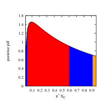
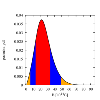
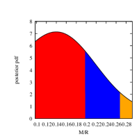
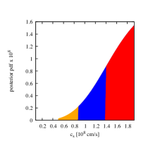
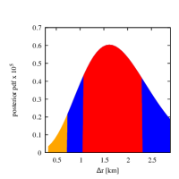
Figure 7: 1D marginalized posteriors for all parameters (black line) and credible intervals for $68.2\%$ (1 $\sigma$, red region), $95.4\%$ (2 $\sigma$, blue region) and $99.7\%$ (3 $\sigma$, orange region).

Given that the model only depends on five parameters and the relative smallness of the parameter space, we can tackle the problem of the computation of the posteriors directly by discretizing the 5-dimensional parameter space in a grid. We use an equidistant grid for $\bar{B}$, $\varepsilon_{\star}X_{c}$, $c_{s}$, $\Delta r$ ans $M/R$ with $40$ points for each parameter. Once the posteriors are known we marginalize over unwanted parameters to obtain 1D plots of the posteriors for each parameter, and 2D plots for each possible couple of different parameters. Finally we obtain credible intervals by ordering the marginalized data in descending order of probability and integrating until the desired $\sigma$ level.

	$\varepsilon_{\star}X_{c}$	$\bar{B}$	$M/R$	$c_{s}$	$\Delta r$
		[$10^{14}$ G]		[$10^{8}$ cm/s]	[km]
max.	$0.09^{+0.46}_{-0.07}$	$21^{+13}_{-10}$	$0.14^{+0.05}_{-0.04}$	$>1.4$	$1.6^{+0.7}_{-0.6}$
median	0.49	48.	0.20	1.0	1.6

Table 5: Maximum values and 1-$\sigma$ intervals of the 1D marginalized posteriors and median values. For the case of $c_{\rm s}$, the maximum value is encountered at the boundary of the interval, so only a 1-$\sigma$ lower bound is given.

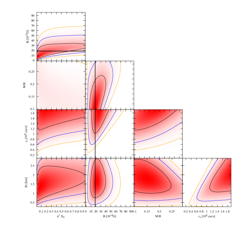
Figure 8: 2D marginalized posteriors for all possible combinations of parameters (color coded) and credible intervals for $68.2\%$ (1 $\sigma$, black line), $95.4\%$ (2 $\sigma$, blue line) and $99.7\%$ (3 $\sigma$, orange line). The thick black line indicates the spin-down estimate of the dipolar magnetic field strength of SGR 1806-20.

Figs. 7 and 8 show 1D and 2D marginalized posteriors for all parameters, respectively, while in Table 5 we give the maximum and median values for each of the parameters based on the 1D marginalized posteriors, including 1-$\sigma$ deviations. The posteriors are spread over a large region of the parameter space. To test what is causing the large errors in the posteriors, we performed an analysis reducing all systematic and observational errors to $1\%$ and obtained qualitatively similar results and errors in the posteriors. This implies that the errors are dominated by the fact that we are using a model with $5$ parameters to fit only two observational data. Actually, in about $8\%$ of the volume of the parameter space we find QPO frequencies that match both observations with 1-$\sigma$ confidence. This indicates that there is a large degree of degeneracy in the parameter space, and hence the posteriors produce only weak constraints.

The value of the magnetic-field strength for SGR 1806-20 based on our Bayesian analysis, $\bar{B}=2.1^{+1.3}_{-1.0}\times 10^{15}\,$G, is in remarkable agreement with its value based on the measured period spin-down $\bar{B}=2\times 10^{15}$ G (Woods et al., 2007). This may be an indication that the magnetic field is predominantly dipolar also inside the star and no high-order multipoles are present. The value of $\varepsilon_{\star}X_{c}=0.09^{+0.46}_{-0.07}$ is incompatible with a normal fluid core, i.e. we require a significant part of the matter to be superfluid in our model. In fact, the median value is close to the values theoretically predicted for completely superfluid models $\varepsilon_{\star}^{0}X_{c}^{0}=0.046$ (Douchin & Haensel, 2001).

Our analysis also favours a small compactness of $M/R\lesssim 0.19$. Assuming a $1.4$ M_⊙ neutron star, this would imply a relatively stiff EoS. In addition, the mass of the object is likely to not be close to the maximum mass allowed by the EoS, because high-mass neutron stars are usually more compact. For example, if we consider the additional constraints to the EOS by Lattimer & Steiner (2014), our compactness restricts the mass of the neutron star to be in the interval $0.7-1.5~{}M_{\odot}$. Finally, both the inferred shear speed $c_{s}>1.4\times 10^{8}\,$cm/s and crust thickness $\Delta r=1.61^{+0.7}_{-0.6}\,$km are on the upper range of the expectations of theoretical models (Steiner & Watts, 2009; Sotani et al., 2008).

4.4 Potential conflicts with observations

The detection of very similar frequencies in the normal bursts of J1550-5418 (Huppenkothen et al., 2014a) and in the giant flares of SGR 1806-20 and SGR 1900+14 poses a problem for their interpretation as magneto-elastic oscillations: Why do all three magnetars have very similar oscillations frequencies while their magnetic field strength estimates differ by almost one order of magnitude, $\bar{B}_{J1550}\sim 3.2\times 10^{14}\,$G and $\bar{B}_{1806}\sim 2\times 10^{15}\,$G? The frequencies of magneto-elastic oscillations are expected to scale with the magnetic-field strength like Eq. (14). Our model thus predicts significantly higher frequencies for SGR 1806-20 than for SGR 1900+14, which in turn should have higher frequencies than J1550-5418. Indeed, SGR 1900+14 ($28\,$Hz and $84\,$Hz) has slightly lower frequencies compared to SGR 1806-20 ($30\,$Hz and $92\,$Hz). However, the difference is smaller than expected from Eq. (13). Within our model, the similar frequencies for different magnetic field strengths may still be explained by the following reasons: i) According to Eq. (14), different masses and thus different compactnesses of the neutron stars lead to different frequencies. The maximal allowed difference, depending on the compactness of the particular models, is a factor of roughly $2.5$. ii) Magnetic-field configurations different from the assumed dipolar-dominated configuration may influence the oscillations significantly. There may be strong toroidal fields whose influence on the oscillations have not been studied in sufficient detail yet. Higher order multipoles are unlikely, because they would shift the frequencies to too high values (Gabler et al., 2013b). iii) The spin-down estimate of the magnetic field strength is only accurate to a factor of 2 in the best case. iv) The similar frequencies may belong to different overtones and not to the fundamental oscillation. To break this degeneracy, a clear identification of the observed magneto-elastic oscillation is necessary. Unfortunately, the observational data is yet insufficient to unambiguously determine which overtone or fundamental mode frequency can be associated with an observed frequency, i.e. there is still no unambiguous pattern in the frequency spacing of the QPOs. Recent work on detecting QPOs in normal burst of magnetars is thus very promising (Huppenkothen et al., 2014a; Huppenkothen et al., 2014c) and we strongly encourage further studies in this direction.

During the late phase of the writing of this paper a re-analysis of the observational data of the two giant flares of SGR 1806 and SGR 1900 was presented by Pumpe et al. (2017). Unfortunately, they do not confirm the previously reported frequencies, but find new potential signals at $9.2\,$Hz and $7.7\,$Hz, respectively. They do not comment on the high-frequency QPOs above $150\,$Hz. Assuming that the newly found low frequency QPO at $9.2\,$Hz is the fundamental magneto-elastic QPO (${}^{2}U_{2}$), we can perform perform the same Bayesian analysis to see how the results change with this different identification. We have considered two alternative cases, one in which we identify the $625$ Hz QPO as the high frequency QPO (${}^{2}t_{1}$) and a second case in which we do not consider any high frequency QPO. The results for the maximum values of the 1D marginalised posteriors are summarised and compared to our previous results in Table 6. The estimates for the magnetic field strength in all cases are still compatible with the spin-down estimate. With the lower frequency of $9.2\,$Hz, our estimates for the crust thickness and shear speed become lower than before, while the compactness becomes larger. $\varepsilon_{\star}X_{c}$ is significantly larger than previously estimated, but it is still consistent with a large fraction of the core being superfluid. Thus, it is of great importance to clarify, which frequencies are present in the signal.

${}^{2}U_{2}$	${}^{2}t_{1}$	$\varepsilon_{\star}X_{c}$	$\bar{B}$	$M/R$	$c_{s}$	$\Delta r$
			[$10^{14}$ G]		[$10^{8}$ cm/s]	[km]
$29$ Hz	$625$ Hz	$0.09^{+0.46}_{-0.07}$	$21^{+13}_{-10}$	$0.14^{+0.05}_{-0.04}$	$>1.4$	$1.6^{+0.7}_{-0.6}$
$9.2$ Hz	$625$ Hz	$0.5^{+0.4}_{-0.2}$	$14^{+10}_{-7}$	$>0.2$	$>1.2$	$1.1^{+0.6}_{-0.5}$
$9.2$ Hz	-	$0.4^{+0.4}_{-0.2}$	$11^{+10}_{-7}$	$>0.2$	$>1.0$	-

Table 6: Maximum values and 1-$\sigma$ intervals (or 1-$\sigma$ lower limits) of the 1D marginalised posteriors, for three different identifications of the QPOs in giant flares: the same as in table 5 (upper row), using $9.2$ Hz as low frequency QPO instead of $29$ Hz (middle row), and using only $9.2$ Hz (lower row). In the latter case, there are no constrains on $\Delta r$.

5 Conclusions

In this paper we have discussed torsional oscillations of highly magnetized neutron stars (magnetars). Those are described by means of two-dimensional, magneto-elastic-hydrodynamical simulations. Our model of superfluid magneto-elastic oscillations is able to explain both the low- and high-frequency QPOs observed in magnetars. In particular we have shown that the analysis of these oscillations provides constraints on the breakout magnetic-field strength, on their fundamental frequency, and on the frequency of a particularly excited overtone. We have also shown how to use this information to constraint properties of high-density matter in neutron stars in general, employing Bayesian analysis.

Our model-dependent Bayesian posterior estimates for SGR 1806-20 give a magnetic-field strength $\bar{B}=2.1^{+1.3}_{-1.0}\times 10^{15}\,$G and a superfluid parameter $\varepsilon_{\star}X_{c}=0.09^{+0.46}_{-0.07}$, which encodes entrainment and proton fraction. The uncertainties given are 1-$\sigma$ error bars from the Bayesian inference. Both of these values agree remarkably well with observational and theoretical expectations, respectively. We have further obtained posterior estimates that favour a low value of the compactness of the star, $M/R\lesssim 0.19$, indicating a relatively stiff EoS and/or low mass neutron star, a relatively high shear speed at the base of the crust, $c_{s}>1.4\times 10^{8}\,$cm/s, and a thick crust with $\Delta r=1.61^{+0.7}_{-0.6}\,$km.

The main source of uncertainties in our analysis is neither the accuracy of our models nor of the observations, but the lack of observational data. We are constraining five parameters with only two observational data. As a consequence, there is a large degeneracy in the parameter space, which produces large uncertainties in the posteriors. Future X-ray observatories could provide more data, either detecting QPOs in the more frequent intermediate flares or even looking to extra-galactic giant flares. It still has to be clarified how to stack data from different objects in a Bayesian analysis to produce meaningful and tight constraints on the properties of neutron star interiors. One of the problems is the use of parameters that depend on the particular object under consideration (magnetic field strength and configuration, and crust thickness $\Delta r$), which will have to be substituted by general properties, which hold for all neutron stars with future QPO detections. This work is only a proof-of-principle that it is possible to extract information from QPOs. The detailed multi-object analysis will be performed elsewhere.

Our model is however not complete, as it still does not include the possibility of the protons to be superconducting (which may be destroyed due to the ultra-strong magnetic fields in magnetars) nor the coupling of toroidal and poloidal oscillations, that may change the QPO spectrum. Therefore, there is room to improve our current interpretation of the QPOs observed in magnetar giant flares. Nevertheless, we have shown how a systematic analysis of the coupled magneto-elastic oscillations can help to constrain the properties of matter at nuclear densities. This is a significant improvement over previous studies that only took into account pure crustal shear modes. Furthermore, the constraints derived in this paper are general, in the sense that they are based on general physical properties like the breakout of the oscillations, the matching of the fundamental oscillation, and the presence of a particular high-frequency QPO. Therefore, the procedure described here to obtain the constraints will still be valid in future improvements of the model (including e.g. superconductivity) and only the particular values of the quantities may change.

A main constraint derived in this work is the breakout of the oscillations from the core to the surface which depends on the magnetic-field strength and on the $\varepsilon_{\star}X_{c}$ parameter. By identifying the magnetic-field strength below which no QPOs are observed in magnetars, one could fix $\bar{B}_{\mathrm{breakout}}$ observationally and use Eq. (15) to determine the superfluid properties ($\varepsilon_{\star}X_{c}$) for a given magnetic-field configuration. To make this kind of constraints possible, observations like those of Huppenkothen et al. (2014a); Huppenkothen et al. (2014c) are indispensable and more work in this direction is highly encouraged. Another important open question is how the oscillations of the neutron star may modulate the emission. To understand the modulation mechanism is essential to estimate the amplitude of the oscillations and to compare with the properties of the observed QPOs. We plan to address these issues in further work.

References

- Akmal et al. (1998) Akmal A., Pandharipande V. R., Ravenhall D. G., 1998, Phys. Rev. C, 58, 1804
- Andersson et al. (2009) Andersson N., Glampedakis K., Samuelsson L., 2009, MNRAS, 396, 894
- Bocquet et al. (1995) Bocquet M., Bonazzola S., Gourgoulhon E., Novak J., 1995, A&A, 301, 757
- Cerdá-Durán et al. (2008) Cerdá-Durán P., Font J. A., Antón L., Müller E., 2008, A&A, 492, 937
- Cerdá-Durán et al. (2009) Cerdá-Durán P., Stergioulas N., Font J. A., 2009, MNRAS, 397, 1607
- Chamel (2012) Chamel N., 2012, Phys. Rev. C, 85, 035801
- Chamel & Haensel (2008) Chamel N., Haensel P., 2008, Living Reviews in Relativity, 11
- Colaiuda & Kokkotas (2011) Colaiuda A., Kokkotas K. D., 2011, MNRAS, 414, 3014
- Colaiuda et al. (2009) Colaiuda A., Beyer H., Kokkotas K. D., 2009, MNRAS, 396, 1441
- Deibel et al. (2014) Deibel A. T., Steiner A. W., Brown E. F., 2014, Phys. Rev. C, 90, 025802
- Douchin & Haensel (2001) Douchin F., Haensel P., 2001, A&A, 380, 151
- Duncan (1998) Duncan R. C., 1998, ApJ, 498, L45
- Gabler et al. (2011) Gabler M., Cerdá Durán P., Font J. A., Müller E., Stergioulas N., 2011, MNRAS, 410, L37
- Gabler et al. (2012) Gabler M., Cerdá-Durán P., Stergioulas N., Font J. A., Müller E., 2012, MNRAS, 421, 2054
- Gabler et al. (2013a) Gabler M., Cerdá-Durán P., Stergioulas N., Font J. A., Müller E., 2013a, Physical Review Letters, 111, 211102
- Gabler et al. (2013b) Gabler M., Cerdá-Durán P., Font J. A., Müller E., Stergioulas N., 2013b, MNRAS, 430, 1811
- Gabler et al. (2014a) Gabler M., Cerdá-Durán P., Font J. A., Stergioulas N., Müller E., 2014a, Astronomische Nachrichten, 335, 240
- Gabler et al. (2014b) Gabler M., Cerdá-Durán P., Stergioulas N., Font J. A., Müller E., 2014b, MNRAS, 443, 1416
- Gabler et al. (2016) Gabler M., Cerdá-Durán P., Stergioulas N., Font J. A., Müller E., 2016, MNRAS, 460, 4242
- Glampedakis et al. (2006) Glampedakis K., Samuelsson L., Andersson N., 2006, MNRAS, 371, L74
- Glampedakis et al. (2011) Glampedakis K., Andersson N., Samuelsson L., 2011, MNRAS, 410, 805
- Hambaryan et al. (2011) Hambaryan V., Neuhäuser R., Kokkotas K. D., 2011, A&A, 528, A45+
- Huppenkothen et al. (2014a) Huppenkothen D., et al., 2014a, ApJ, 787, 128
- Huppenkothen et al. (2014b) Huppenkothen D., Watts A. L., Levin Y., 2014b, ApJ, 793, 129
- Huppenkothen et al. (2014c) Huppenkothen D., Heil L. M., Watts A. L., Göğüş E., 2014c, ApJ, 795, 114
- Israel et al. (2005) Israel G. L., et al., 2005, ApJ, 628, L53
- Lattimer & Steiner (2014) Lattimer J. M., Steiner A. W., 2014, ApJ, 784, 123
- Levin (2006) Levin Y., 2006, MNRAS, 368, L35
- Levin (2007) Levin Y., 2007, MNRAS, 377, 159
- Messios et al. (2001) Messios N., Papadopoulos D. B., Stergioulas N., 2001, MNRAS, 328, 1161
- Passamonti & Lander (2013) Passamonti A., Lander S. K., 2013, MNRAS, 429, 767
- Passamonti & Lander (2014) Passamonti A., Lander S. K., 2014, MNRAS, 438, 156
- Passamonti & Pons (2016) Passamonti A., Pons J. A., 2016, MNRAS, 463, 1173
- Piro (2005) Piro A. L., 2005, ApJ, 634, L153
- Pumpe et al. (2017) Pumpe D., Gabler M., Steininger T., Enßlin T. A., 2017, preprint, (arXiv:1708.05702)