Third-order optical conductivity of an electron fluid

Abstract

We derive the nonlinear optical conductivity of an isotropic electron fluid at frequencies below the interparticle collision rate. In this regime, governed by hydrodynamics, the conductivity acquires a universal form at any temperature, chemical potential, and spatial dimension. We show that the nonlinear response of the fluid to a uniform field is dominated by the third-order conductivity tensor $\sigma^{(3)}$ whose magnitude and temperature dependence differ qualitatively from those in the conventional kinetic regime of higher frequencies. We obtain explicit formulas for $\sigma^{(3)}$ for Dirac materials such as graphene and Weyl semimetals. We make predictions for the third-harmonic generation, renormalization of the collective-mode spectrum, and the third-order circular magnetic birefringence experiments.

I Introduction

In typical metals and semiconductors electrons experience frequent collisions with impurities and phonons. The combined rate $\Gamma_{d}=\Gamma_{dis}+\Gamma_{ph}$ of these collisions far exceeds the rate $\Gamma_{ee}$ of electron-electron scattering. However, in several pure materials the opposite case $\Gamma_{d}\ll\Gamma_{ee}$ has recently shown to be possible in a range of temperatures. Under such conditions Gurzhi (1968); Andreev et al. (2011) electrons behave as a fluid that obeys hydrodynamic equations. Landau and Lifshitz (1987) Evidence for the hydrodynamic behavior has been obtained from dc transport experiments with two-dimensional (2D) electron gases in GaAs de Jong and Molenkamp (1995), graphene, Bandurin et al. (2016); Crossno et al. (2016); Krishna Kumar et al. (2017) and a quasi-2D metal $\mathrm{PdCoO_{2}}$. Moll et al. (2016) These discoveries stimulated many theoretical studies. Müller et al. (2008, 2009); Phan et al. ; Forcella et al. (2014); Briskot et al. (2015); Narozhny et al. (2015); Principi and Vignale (2015a, b); Sun et al. (2016); Lucas et al. (2016); Lucas (2017); Sun et al. ; Guo et al. (2017) The conceptual simplicity of hydrodynamics arises from dealing with only a few degrees of freedom: the local temperature $T(\mathbf{r},t)$, chemical potential $\mu(\mathbf{r},t)$, and the flow velocity $\mathbf{u}(\mathbf{r},t)$. The complicated many-body collisions need not be considered explicitly. In our previous paper Sun et al. we used this hydrodynamic formalism to calculate the electrodynamic response of an electron fluid, in particular, its linear and second-order nonlinear optical conductivities. The magnitude and functional form of these quantities in the hydrodynamic regime of frequencies $\omega\ll\Gamma_{ee}$ were shown to differ qualitatively from their counterparts in the conventional kinetic regime $\omega\gg\Gamma_{ee}$. Here we continue this line of investigation by addressing the third-order nonlinearity, which controls, e.g., the third-harmonic generation (Fig. 1), the Kerr effect, and four-wave mixing.

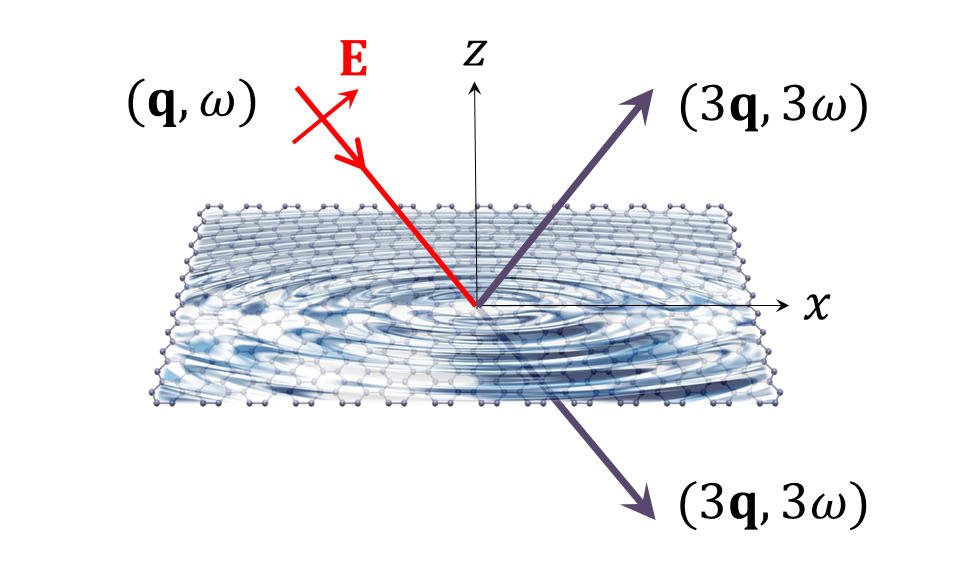
Figure 1: Illustration of the third-order optical nonlinearity in graphene.

One reason why the third-order nonlinearity warrants attention is dictated by the symmetry. In general, the electrodynamic response of a conductor is characterized by the tensors $\sigma^{(n)}$ describing the components of the induced current proportional to the $n$th-power of the electric field. (The definition of these tensors is given in Sec. II). Unless the field is very strong, the nonlinear response of a material lacking the inversion symmetry is dominated by the second-order conductivity $\sigma^{(2)}$. However, in centro-symmetric systems, such as graphene, $\sigma^{(2)}$ must vanish if the electric field is uniform, in which case the third-order conductivity $\sigma^{(3)}$ becomes more important.

As we show below in this paper, the derivation of the nonlinear conductivities is straightforward within a certain model that we call the Dirac fluid. This model is simple yet flexible enough to describe several types of solid-state materials. The model assumes that the quasiparticles of the system behave as Dirac fermions with the energy-momentum dispersion $\varepsilon^{2}(\mathbf{p})=m^{2}v^{4}+\mathbf{p}^{2}v^{2}$. The massless case $m=0$ corresponds to electrons in graphene; the massive case $m>0$ is a reasonable approximation for narrow-gap semiconductors. Neglecting fermion-fermion interactions, one can readily compute the equilibrium thermodynamic parameters of this system, Müller et al. (2008, 2009); Briskot et al. (2015); Sun et al. (2016, ) such as the pressure $P=P(\mu,T)$ and the energy density $n_{E}=n_{E}(\mu,T)$. The crucial simplification of the Dirac model is that the energy-momentum tensor of the moving fluid can be derived from that of the static one by a Lorentz transformation with $v$ in lieu of the speed of light $c$. [In the noninteracting case, the moving fluid is defined as the Fermi distribution of quasiparticles with the Doppler-shifted energies $\varepsilon(\mathbf{p})-\mathbf{p}\mathbf{u}$.] The Lorentz invariance ensures that the hydrodynamic equations of a Dirac fluid have a simple “relativistic” form. Landau and Lifshitz (1987); Müller et al. (2008, 2009); Briskot et al. (2015); Narozhny et al. (2015); Sun et al. (2016, ) Precisely because $v\neq c$, the solid-state systems with real Coulomb interactions are not truly Lorentz-invariant. However, the Dirac fluid should be a reasonable approximation if the Coulomb interactions are not too strong, so that $P$ and $n_{E}$ are dominated by the kinetic energy. Besides graphene, examples of such Dirac fluids may include the surface states of topological insulators and three-dimensional Dirac/Weyl semimetals.

Note that the hydrodynamics regimes probed by recent dc transport experiments Bandurin et al. (2016); Crossno et al. (2016); Krishna Kumar et al. (2017) is less than $1$-$\mathrm{THz}$ wide. If one wants to expand it toward higher $\omega$, it is necessary to increase $\Gamma_{ee}$, which can be done by raising electron temperature $T$ (Fig. 2). This must be done without heavily increasing the electron-phonon scattering rate $\Gamma_{ph}$, which is also temperature-dependent. One possible solution Sun et al. is to work with (steady or transient) states where electrons are “hot” but lattice stays “cold.” Such nonequilibrium states can be created by optical pumping or electric-current heating.

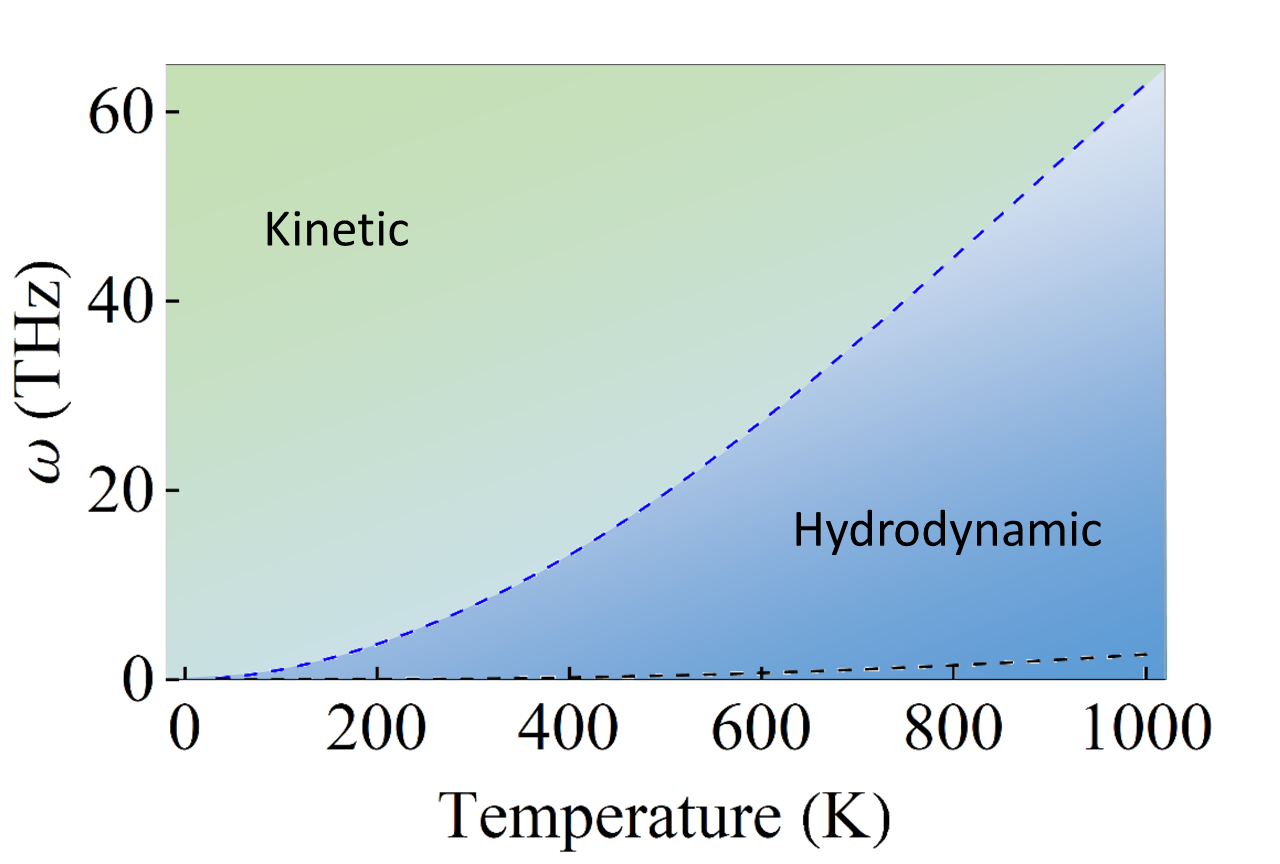
Figure 2: (Schematic) Kinetic and hydrodynamic domains in the frequency-temperature diagram of graphene for the carrier density $n=10^{12}\,\mathrm{cm^{-2}}$, corresponding to the zero-temperature chemical potential $\mu(n,0)=0.12\,\mathrm{eV}$. The (upper) dashed line separating the two regimes is $\omega=\Gamma_{ee}(n,T)$. The lower dashed line is the momentum relaxation rate due to electron scattering by acoustic and $A_{1}^{\prime}$ zone-boundary phonons.

At frequencies $\omega>\Gamma_{ee}$ where the hydrodynamic theory fails, the response of the system is better described by more conventional approaches, e.g., the Boltzmann kinetic equation neglecting electron-electron collisions. Among the Dirac materials, graphene has been the most common target of such calculations. Nonlinear conductivity of graphene has been addressed in many theoretical studies. Mikhailov (2007, 2011); Gullans et al. (2013); Cheng et al. (2014); Yao et al. (2014); Cheng et al. (2015); Mikhailov (2016); Tokman et al. (2016); Cheng et al. (2017); Manzoni et al. ; Wang et al. (2016); Rostami et al. (2017); Sun et al. As discussed in our previous work Sun et al. , the differences between the hydrodynamic and kinetic regimes (Fig. 2) becomes conspicuous at temperatures $T$ exceeding the chemical potential $\mu$, where graphene contains two types of carriers, electrons and thermally excited holes. In the kinetic regime, electrons and holes tend to move in opposite directions when driven by the electric field. Their contributions to the electric current add up. In the hydrodynamic regime, due to frequent interparticle collisions, all the carriers tend to move together. Hence, the electron and hole currents partially cancel. As a consequence, there is an increased effective mass per unit charge, resulting in reduced linear and second-order nonlinear conductivities.Sun et al. In this work we show that the third-order electrodynamic response also exhibits distinct behaviors in the two regimes, in accord with this physical picture.

The remainder of the paper is organized is follows. Section II gives a summary of our main results such as the analytical formula for the third-order nonlinear conductivity of an isotropic Dirac fluid. This formula is simple and universal. It is valid for any mass $m$, chemical potential $\mu$, temperature $T$, and space dimension $d$ if momentum nonconserving processes can be neglected, $\Gamma_{d}\to 0$. We also discuss the general form of the higher nonlinear conductivities tensors $\sigma^{(n)}$ of odd order $n$. In Sec. III we introduce the relativistic hydrodynamic equations and apply them to the massless case, such as graphene. In Sec. IV we give the derivation of $\sigma^{(3)}$, including the case of an external applied magnetic field. In Sec. V we apply our results for $\sigma^{(3)}$ to computing the third harmonic generation. In Sec. VI we discuss the Kerr effect and its influence on the hydrodynamic collective modes of the fluid. In Sec. VII we compute the magnetic-field-induced third-order circular birefringence. The concluding remarks are given in Sec. VIII. Appendix A provides a summary of the analytical expressions for the thermodynamic quantities of a massless Dirac fluid. Appendix B outlines the derivation of $\sigma^{(3)}$ for a more realistic case of a finite scattering rate $\Gamma_{d}$.

II Main results

The $N$th order nonlinear ac conductivity $\sigma^{(N)}$ is defined as a rank $(1,N)$ tensor which maps electric fields to the $N$th order electrical current

$$j_{i}^{(N)}(\mathbf{q},\omega) =\sum\limits_{\nu_{1}...\nu_{N}}\,\sum\limits_{(\mathbf{q}_{1},\omega_{1}),(\mathbf{q}_{2},\omega_{2})\,\ldots(\mathbf{q}_{N},\omega_{N})}\delta\left(\sum_{a}^{N}(\mathbf{q}_{a},\omega_{a})-(\mathbf{q},\omega)\right)$$

$$\sigma^{(N)}_{i\nu_{1}...\nu_{N}}(\mathbf{q}_{1},\omega_{1},\mathbf{q}_{2},\omega_{2}\,\ldots,\mathbf{q}_{N},\omega_{N})$$

$$E_{\nu_{1}}\left(\mathbf{q}_{1},\omega_{1}\right)E_{\nu_{2}}\left(\mathbf{q}_{2},\omega_{2}\right)...E_{\nu_{N}}\left(\mathbf{q}_{N},\omega_{N}\right)\,.$$ (1)

The even, e.g., second order conductivities vanish at zero momentum in centro-symmetric systems. We therefore focus on odd order (e.g., $N=3$) conductivities and disregard $\mathcal{O}(q^{2})$ nonlocal corrections.

For a general $d$-dimensional charged ideal fluid with $O(d)$ (rotation and reflection) symmetry, the $N$th order nonlinear optical conductivity is found to be

$$\sigma^{(N)}_{i\,\nu_{1}\nu_{2}\,\ldots,\nu_{N}}=\frac{iD_{h}^{(N)}}{\omega_{1}\omega_{2}\,\ldots,\omega_{N}}\Delta_{i\,\nu_{1}\nu_{2}...\nu_{N}}\,$$ (2)

where

$$\Delta_{i\,\nu_{1}\nu_{2}...\nu_{N}}=\delta_{i\,\nu_{1}}\delta_{\nu_{2}\nu_{3}}...\delta_{\nu_{N-1}\nu_{N}}+\mathrm{permutations}\,$$ (3)

is the totally symmetric rank $N+1$ tensor which is the sum of the $N!!$ isotropic tensors. Note that $O(d)$ symmetry only requires that $\sigma^{(N)}$ is a linear combination of the isotropic tensors. As we will show later, due to the additional condition of thermal equilibrium in the hydrodynamic regime, $\sigma^{(N)}$ can only be proportional to the totally symmetric rank $N+1$ tensor $\Delta_{i,\nu_{1}\nu_{2}\,\ldots,\nu_{N}}$. The hydrodynamic $N$th order optical weight $D_{h}^{(N)}$ should be understood as a thermodynamic quantity which is generally unknown.

Applied to the Dirac fluid, which has (quasi) Lorentz symmetry, the linear optical conductivity is recovered as $\sigma_{ij}=\frac{iD_{h}/\pi}{\omega}\delta_{ij}$ where the hydrodynamic Drude weight is $D_{h}=\pi ne^{2}/m^{\ast}$ (see, e.g., Supplemental material of Ref. Sun et al., ). The most important result of this paper is that the third-order nonlinear optical conductivity is given by

$$\sigma^{(3)}_{ilmn} =\frac{iD_{h}^{(3)}}{\omega_{1}\omega_{2}\omega_{3}}\Delta_{ilmn}$$

$$=\frac{iD_{h}^{(3)}}{\omega_{1}\omega_{2}\omega_{3}}\left(\delta_{il}\delta_{mn}+\delta_{im}\delta_{ln}+\delta_{in}\delta_{lm}\right)\,.$$ (4)

Here the third-order optical weight

$$D_{h}^{(3)}=\frac{1-C_{\mathrm{ise}}}{3!}\frac{e^{4}n}{m^{\ast 3}v^{2}}=\frac{1-C_{\mathrm{ise}}}{3!}\frac{W}{\rho^{4}v^{4}}\left(\frac{D_{h}}{\pi}\right)^{4}\,.$$ (5)

is expressed in terms of thermodynamic quantities and the asymptotic velocity $v$. These quantities are defined in Sec. III below.

III Hydrodynamics

III.1 Hydrodynamic equations

The hydrodynamic equations for an ideal relativistic charged fluid areLandau and Lifshitz (1987)

$$\partial_{\mu}T^{\mu\nu}=J_{\mu}F^{\nu\mu},\quad\partial_{\mu}J^{\mu}=0\,$$ (6)

where $T^{\nu\mu}$ is the energy-momentum tensor, $F^{\nu\mu}$ is the electromagnetic field tensor, and

$$J^{\mu}=(\rho v,\,\mathbf{j}\,),\qquad\mathbf{j}=(j_{x},j_{y},j_{z})$$ (7)

is the four-current and its spatial part, respectively. By ideal we mean a fluid with vanishing viscosity and thermal conductivity. Although a “covariant” notation is implemented, Eq. (6) holds even for systems without Lorentz symmetry because the conservation of the stress tensor requires only the translational symmetry. The form of stress tensor for a general interacting fluid is unknown; however, for Lorentz-invariant systems, i.e., Dirac fluids, the stress tensor is related to thermodynamic quantitiesLandau and Lifshitz (1987)

$$T^{\mu\nu}=Wu^{\mu}u^{\nu}-Pg^{\mu\nu}\,.$$ (8)

The four-current is related to the proper charge density through $J^{\mu}=\rho_{0}u^{\mu}=\rho_{0}\gamma(v,\,\mathbf{u})=\rho(v,\,\mathbf{u})$ where $\gamma=1/\sqrt{1-u^{2}/v^{2}}$. In solid state system, the $v$ is the asymptotic velocity such that electrons have a Dirac-like energy-momentum dispersion $\varepsilon_{p}^{2}=(pv)^{2}+(mv^{2})^{2}$. The thermodynamic quantities, the proper charge density $\rho_{0}=en_{0}$, the enthalpy density $W$ and the pressure $P$ are all defined in the fictitious proper frame moving with the local liquid. Note that $n\equiv\rho/e$ is defined as the effective charge carrier density and is in general not the same as particle density. For example, in graphene at high temperature, there are both electrons and holes, and $n$ will be the number of electrons minus the number of holes. We define the hydrodynamic effective mass as $m^{\ast}\equiv W/(nv^{2})$. And we define

$$C_{\mathrm{ise}}=\frac{n}{W}\left(\frac{\partial W}{\partial n}\right)_{\mathrm{ise}}-1=\frac{n}{W}\left(\frac{\partial P}{\partial n}\right)_{\mathrm{ise}}=\frac{1}{m^{\ast}\!v^{2}}\left(\frac{\partial P}{\partial n}\right)_{\mathrm{ise}}$$ (9)

as the dimensionless bulk isentropic modulus of the electron fluidSun et al. . For example, it has the value $1/d$ for massless Dirac particles in space dimension $d$. Out of the three thermodynamic quantities $W$, $P$ and $\rho_{0}$ only two are independent. Thus the independent variables are any two thermodynamic quantities and the local flow velocity $\mathbf{u}$. This set of equations (6) is closed.

Alternatively, these hydrodynamic equations can be derived from the Boltzmann kinetic equation with the inter particle collision integral but neglecting the many-body interaction correction to the thermodynamic quantities, as shown in Ref. Briskot et al., 2015 and also the covariant version in Appendix C.

From Eq. (8), the first part of Eq. (6) could be written in another form

$$Wu^{\mu}\partial_{\mu}u^{\nu}-\partial^{\nu}P+u^{\nu}u^{\mu}\partial_{\mu}P=J_{\mu}F^{\nu\mu}\,.$$ (10)

Separating the time and spatial components in a proper way, Eq. (6) has another form

$$(\partial_{t}+u_{k}\partial_{k})u_{i}=\,$$

$$\frac{1}{\gamma^{2}W}\left(-\partial_{i}P-u_{i}\partial_{t}P+\rho E_{i}+\rho\epsilon_{ikl}u_{k}\frac{v}{c}B_{l}-u_{i}\mathbf{j}\cdot\mathbf{E}\right)\,,$$ (11)

$$\partial_{t}(n_{E})+\nabla(\gamma^{2}W\mathbf{u})=\mathbf{j}\cdot\mathbf{E}\,,$$ (12)

$$\partial_{t}\rho+\nabla\cdot\mathbf{j}=0\,.$$ (13)

where $n_{E}=\gamma^{2}W-P$ is the energy density of the electrons (relative to zero doping and temperature case), and $n_{E0}=W-P$ is the same quantity but in the proper frame. Equation (11) is the relativistic version of the Euler equation, Eq. (12) is the conservation of the energy current and Eq. (13) is the conservation of the charge current. Terms due to viscosity and dissipative thermal conductivity are neglected because they affect the conductivities only through $O(q^{2})$ terms. To simplify the notations, the asymptotic velocity has been taken to be $v=1$ except for the Lorentz force term due to the magnetic field $\mathbf{B}$. Note that the magnetic field is related to the electric one by $\nabla\times\mathbf{E}=-c^{-1}\partial_{t}\mathbf{B}$. Since we neglect finite-$q$ effects in this work, we must set $\nabla\times\mathbf{E}=0$, so that the magnetic field is considered time-independent.

Starting from Eqs. (11), (12) and (13) we can compute the linear and in principle, any higher-order nonlinear optical conductivities $\sigma^{(N)}$ by expanding all the dynamic variables in powers of the electric field $\mathbf{E}$. This procedure and its results are presented in the following sections.

III.2 Hydrodynamic regime of graphene

Hydrodynamic regime is not a phase of matter but a domain of frequency-momentum diagram [see, e.g., Fig. 1 of Ref. Sun et al., ] where the hydrodynamic equations work well as an effective theory. This regime is defined by inequalities $\Gamma_{d},\,\omega\ll\Gamma_{ee}$ and $q\ll l_{ee}^{-1}$, which can be satisfied in some pure solid-state systems. The electron-electron collision rate $\Gamma_{ee}(n,T)$ that sets the upper bound on the hydrodynamic regime depends on temperature and doping level of the electron system. For example, in graphene, $\Gamma_{ee}$ scales as $\sim\ln(2\mu/T)(T^{2}/\mu)$ at low $T$ and as $\sim\alpha^{2}T$ at $T\gg\mu$ with $\alpha\sim 1$. For a rough estimate, we connect these two formulas by a naive interpolation with the relative weights $\mu/(T+\mu)$ and $T/(T+\mu$), respectively. The corresponding boundary of the hydrodynamic domain (blue region) is shown by the upper dashed line in Fig. 2. The other important scattering rate shown in the same Figure is $\Gamma_{d}$. For ultra clean graphene encapsulated in hexagonal boron nitride (hBN), the major contribution to $\Gamma_{d}$ is the electron-phonon scattering $\Gamma_{ph}$. The electron-phonon scattering suppresses the hydrodynamic behavior if $\Gamma_{ph}>\Gamma_{ee}$. However, our theoretical estimation of $\Gamma_{ph}$ and $\Gamma_{ee}$ indicates that the hydrodynamic regime of graphene is fairly large, as shown in Fig. 2. Furthermore, in a nonequlibrum situation where the electron system is at high temperature $T$ while the lattice temperature $T_{l}$ remains low, $\Gamma_{ee}$ is enhanced while the $\Gamma_{ph}=\Gamma_{ph}(T_{l},T,n)$ remains small, and so the hydrodynamic window could be wider. Such a nonequlibrum situation can be realized either through optical pumping Ni et al. (2016) or by Joule heating due to an electric current. Son et al. (2018)

Recent experiments Bandurin et al. (2016); Crossno et al. (2016); Krishna Kumar et al. (2017); Moll et al. (2016) explored the dc transport in several pure 2D conductors in the regime $\Gamma_{d}\ll\Gamma_{ee}$, i.e., near the horizontal axis $\omega=0$ of Fig. 2. These measurements revealed signatures of viscous electron flow, which manifest themselves through a combination of high viscosity $\nu=v^{2}/\Gamma_{ee}$ and geometrical restriction on the flow. Because of the particular focus of these studies, the lower viscosity, higher temperature regime was labeled as nonhydrodynamic. From our point of view, viscosity is just one of very many hydrodynamic phenomena rather than its essential element. Actually, in the high-temperature regime, where the electron-hole plasma becomes a more perfect fluid,Müller et al. (2009) hydrodynamic effects should be of crucial importance. They are predicted to give dramatically different optical responses compared to the noninteracting kinetic theory. Sun et al.

IV Third-order nonlinear optical conductivity

IV.1 The general charged fluid

Since we neglect the $\mathcal{O}(q^{2})$ nonlocal corrections, $\sigma^{(N)}$ could be derived by simply considering the fluid driven by a uniform electric field. (The dynamic magnetic field $\mathbf{B}$ is zero in this case.) The hydrodynamic equations (6) simplify to

$$\partial_{t}\mathbf{p}=\rho\mathbf{E}\,,\quad\partial_{t}\rho=0\,,\quad\partial_{t}S_{n}=0\,.$$ (14)

where $\mathbf{p}$ is the momentum density and $S_{n}=S/n$ is the entropy per unit charge. The last relation in Eq. (14) comes from the fact that the hydrodynamic flow is isentropic. The second relation in Eq. (14) comes from the charge continuity equation. It entails that the charge density $\rho$ stays constant. In turn, the first relation in Eq. (14) implies that $\mathbf{p}$ is strictly linear in $\mathbf{E}$. If the electric field in the system is composed of Fourier harmonic with amplitudes $\mathbf{E}_{a}$ and frequencies $\omega_{a}$, then the momentum density is

$$\mathbf{p}=\sum_{a=1}^{N}\frac{i}{\omega_{a}}\rho\mathbf{E}_{a}e^{-i\omega_{a}t}\,.$$ (15)

The current density can be treated as a thermodynamic function of $n$, $S_{n}$ and $\mathbf{p}$:

$$\mathbf{j}=\mathbf{j}(n,S_{n},\mathbf{p})\,.$$ (16)

Since particle density and entropy are conserved, the $N$th order current where $N=2m+1$, is just the $N$th order Taylor expansion of $\mathbf{j}$ with respect to $\mathbf{p}$. Due to the isotropy of the fluid, current density must be parallel to the momentum: $\mathbf{j}=j\hat{\mathbf{p}}$. Therefore,

$$j_{i}^{(N)}=\frac{1}{N!}\left(\partial_{p}^{N}j\right)(p^{2})^{m}p_{i}\,.$$ (17)

Using Eq. (15), we find the $N$th order current of frequency $\omega=\sum_{a}^{N}\omega_{a}$ to be

$$j_{i}^{(N)} =\frac{1}{N!}\left(\partial_{p}^{N}j\right)\frac{i(-1)^{m}}{\omega_{1}\omega_{2}\ldots\omega_{N}}\delta_{i\,\nu_{1}}\delta_{\nu_{2}\nu_{3}}...\delta_{\nu_{N-1}\nu_{N}}$$

$$\times E_{1,\nu_{1}}E_{2,\nu_{2}}\ldots E_{N,\nu_{N}}+\mathop{\mathrm{perm}}(1,2,\ldots,N)\,.$$ (18)

Here and below “$\mathrm{perm}$” stands for permutations. Therefore, Eq. (2) is proven with

$$D_{h}^{(N)}=\frac{(-2)^{m}m!}{(N!)^{2}}\left(\partial_{p}^{N}j\right)\,.$$ (19)

IV.2 The Lorentz invariant fluid (Dirac fluid)

As we mentioned above, Eq. (14) implies that the charge density $\rho$ is a constant. From Lorentz invariance, the current is $j_{i}=\rho u_{i}$ and therefore $j^{(3)}_{i}=\rho u^{(3)}_{i}$. The flow velocity $\mathbf{u}$ can be found from its nonlinear relation to the momentum $p_{i}=W\gamma^{2}u_{i}$. The left hand side is linear in electric field, thus the third-order terms on the right hand side must vanish:

$$0=Wu_{i}^{(3)}+W^{(2)}u_{i}^{(1)}+W{u^{(1)}}^{2}u_{i}^{(1)}\,.$$ (20)

It follows that

$$u_{i}^{(3)} =-\frac{W^{(2)}}{W}u_{i}^{(1)}-{u^{(1)}}^{2}u_{i}^{(1)}=-\left(\frac{(\frac{\partial W}{\partial n_{0}})_{S_{n}}n^{(2)}_{0}}{W}+{u^{(1)}}^{2}\right)u_{i}^{(1)}\,.$$ (21)

From the relativistic relation $n=\gamma n_{0}$, we have

$$n_{0}=n\left(1-{u}^{2}/2+O({u}^{4})\right)\,,$$ (22)

Thus $n_{0}^{(2)}=n{u^{(1)}}^{2}/2$ and

$$u_{i}^{(3)} =\frac{1}{2}\left(C_{\mathrm{ise}}-1\right){u^{(1)}}^{2}u_{i}^{(1)}\,.$$ (23)

Therefore, we arrive at

$$j^{(3)}=\rho u^{(3)}=\frac{1}{2}\left(C_{\mathrm{ise}}-1\right)(p/W)^{3}$$ (24)

which renders the third-order optical weight Eq. (5).

IV.3 2D Dirac fluid with a static magnetic field

The uniform hydrodynamic equations with a static magnetic field are

$$\partial_{t}p_{i}=\rho E_{i}+\rho\frac{1}{c}\epsilon_{ijk}u_{j}B_{k}\,,\quad\partial_{t}\rho=0\,,\quad\partial_{t}S_{n}=0\,.$$ (25)

The momentum density $\mathbf{p}$ is no longer strictly linear in $\mathbf{E}$. Below we focus on the 2D case, so the Dirac fluid is on $x$-$y$ plane and the static magnetic field is in the $z$-direction. The linear conductivity is modified to Müller et al. (2008)

$$\sigma_{ij}=\frac{D_{h}/\pi}{\omega^{2}-\omega_{c}^{2}}\left(i\omega\delta_{ij}-\omega_{c}\epsilon_{ij}\right)$$ (26)

where $\epsilon_{ij}$ is the antisymmetric tensor in 2D, and $\omega_{c}=eB/(m^{\ast}c)$ is the hydrodynamic cyclotron frequency. Note that $\omega_{c}$ is in general not equal to the usual cyclotron frequency because the hydrodynamic effective mass $m^{\ast}\equiv W/(nv^{2})$ is not exactly the same as the quasiparticle effective mass in a Fermi liquid. From the Euler equation, the third-order momentum is related to the third-order flow velocity

$$-i\omega_{s}p_{i}^{(3)}=\rho\frac{1}{c}\epsilon_{ijk}u_{j}^{(3)}B_{k}\,.$$ (27)

where $\omega_{s}$ is the frequency of the third-order current (the sum frequency). Together with the relation

$$p_{i}^{(3)}=Wu_{i}^{(3)}+\frac{1}{2}(1-C_{\mathrm{ise}})W(u^{(1)})^{2}u_{i}^{(1)}$$ (28)

we get the equation for the third-order current

$$M_{ij}j_{j}^{(3)}=\frac{1}{2}(1-C_{\mathrm{ise}})\frac{W}{\rho^{3}}(j^{(1)})^{2}j_{i}^{(1)}$$ (29)

where $\hat{M}=-\frac{i}{\omega_{s}}\rho\hat{\sigma}^{-1}$, therefore

$$j_{i}^{(3)} =\frac{1}{2}(1-C_{\mathrm{ise}})\frac{W}{\rho^{4}}i\omega_{s}\sigma_{il}(\omega_{s})\left(j^{(1)}\right)^{2}j_{l}^{(1)}$$

$$=\frac{1}{2}(1-C_{\mathrm{ise}})\frac{W}{\rho^{4}}i\omega_{s}\sigma_{i\alpha}(\omega_{s})\sigma_{\alpha l}(\omega_{1})\sigma_{km}(\omega_{2})\sigma_{kn}(\omega_{3})$$

$$\times E_{1l}E_{2m}E_{3n}+\mathop{\text{perm}}(1,2,3)\,.$$ (30)

The symmetrized third-order conductivity reads

$$\sigma^{(3)}_{ilmn} =\frac{1}{3!\cdot 2}(1-C_{\mathrm{ise}})\frac{W}{\rho^{4}}i\omega_{s}\sigma_{i\alpha}(\omega_{s})\sigma_{\alpha l}(\omega_{1})\sigma_{km}(\omega_{2})\sigma_{kn}(\omega_{3})$$

$$+\mathop{\text{perm}}(1,2,3)(l,m,n)$$ (31)

where $\mathop{\text{perm}}(1,2,3)(l,m,n)$ denotes the $3!=6$ permutations of the indices $(l,m,n)$ together with $(1,2,3)$. Therefore, we have proven that the third-order conductivity $\sigma^{(3)}$ is determined by the linear one $\sigma$.

For moderate magnetic field $\omega_{c}\ll\omega$, and the case of a single frequency $\omega_{1}=\omega_{2}=\omega_{3}=\omega$, we can expand $\sigma^{(3)}$ to linear order in $B$:

$$\sigma^{(3)}_{ilmn}=\frac{iD_{h}^{(3)}}{\omega^{3}}\left[\Delta_{ilmn}+i\frac{4\omega_{c}}{3\omega}\Xi_{ilmn}\right],$$ (32)

where $\Xi_{ilmn}=\delta_{lm}\epsilon_{in}+\delta_{ln}\epsilon_{im}+\delta_{mn}\epsilon_{il}$.

IV.4 Analysis of $\sigma^{(3)}$

The simple tensorial structure of Eq. (4) is a result of rotational symmetry and local equilibrium nature of an ideal charged fluid. For comparison, in the high frequency kinetic/quantum regime of graphene, the tensorial structure of $\sigma^{(3)}$ is more complicated due to contributions from interband transitions and disorder scattering effects. Cheng et al. (2014, 2015); Mikhailov (2016) In the hydrodynamic regime, the interband transitions are suppressed by fast e-e scattering, resulting in the simple expression of Eq. (4).

The magnitude of hydrodynamic $\sigma^{(3)}$ is also different from that of the kinetic theory. Applied to graphene at $T=0$, our result for $D_{h}^{(3)}$ is

$$D_{h}^{(3)}(T=0)=\frac{g}{48\pi}\frac{e^{4}v_{F}}{\hbar^{3}k_{F}}=2D_{k}^{(3)}\,,$$ (33)

which is twice the third-order spectral weight $D_{k}^{(3)}$ from the collisionless Boltzmann transport theory Mikhailov (2016); Cheng et al. (2014); Mikhailov (2007). This difference could be measured by, e.g., third harmonic generation to be discussed in Sec. V.

Comparing the third-order nonlinear response with the usual linear one, we notice that the third-order current is suppressed by the parameter

$$\xi=\left(\frac{-eE/\omega}{m^{\ast}v}\right)^{2}\ll 1\,.$$ (34)

This factor is different in the nonrelativistic and the ultrarelativistic regimes because $m^{*}$ depends on the Fermi momentum $p_{F}$. As a result, in the nonrelativisitic case parameter $\xi$ is smaller by the factor of $(v_{F}/v)^{2}\ll 1$ than the ultrarelativistic case. This factor vanishes for a system with the parabolic dispersion, which corresponds to $v\to\infty$. Indeed, for such a system all nonlinearities at zero $q$ should be absent because of the Galilean invariance (Kohn’s theorem). On the other hand, in graphene at zero temperature, which is an example of the ultrarelativistic system, $m^{\ast}v=p_{F}$, so that $\xi=({\delta p}/{p_{F}})^{2}$. Here $\delta p=-eE/\omega$ has the physical meaning of the amplitude of electron momentum oscillation caused by the electric field.

The third-order conductivity (4) diverges at the zero frequency limit, which is unphysical. In reality, the divergence is curbed by the momentum relaxation rate $\Gamma_{d}$, similar to the first order conductivity. A simple but crude way to include the effect of the momentum relaxation is to change all the frequencies $\omega_{a}$ to $\omega_{a}^{+}=\omega_{a}+i\Gamma_{d}$. However, this approach neglects the increase of entropy density due to momentum relaxation. Thus, special care needs to be taken to compute the true nonlinear dc response, as shown in Appendix B.

V Third harmonic generation

Figure 3: The THG signal as a function of temperature at fixed $n$. The frequency of incident light is $\hbar\omega=\varepsilon_{F}/20$ with $\varepsilon_{F}$ being the zero temperature Fermi energy. The blue curve is the prediction of the hydrodynamic theory Eq. (4), the green curve is from the RPA. Cheng et al. (2015) The observable signal should behave as sketched by the dashed curve.

One quantity we can derive from $\sigma^{(3)}$ [Eq. (4)] is the third harmonic generation (THG) Mikhailov (2016); Giorgianni et al. (2016). Assume the ac electric field of the incident light is in the $x$-direction

$$\mathbf{E}(t)=\hat{x}E(\omega)e^{-i\omega t}+\mathrm{c.c.}$$ (35)

The current, which determines the observable THG signal is

$$\mathbf{j}^{(3)}(t)=\hat{x}\sigma^{(3)}_{xxxx}(\omega,\omega,\omega)E(\omega)^{3}e^{-i3\omega t}+\mathrm{c.c.}$$ (36)

Therefore, $\sigma^{(3)}_{xxxx}(\omega,\omega,\omega)$ represents the magnitude of the THG. This quantity is plotted in Fig. 3 as a function of $T$. Also shown in Fig. 3 is the prediction of the conventional theory based on random-phase approximation (RPA), Cheng et al. (2015); Mikhailov (2016) which is valid in the kinetic regime. The two curves exhibit different behavior. At zero temperature, the hydrodynamic theory predicts the THG signal which is twice that of the kinetic theory. However, since $\Gamma_{ee}=0$ at $T=0$, the electron system much be in the kinetic regime (Fig. 2), and so the actual $\sigma^{(3)}_{xxxx}(\omega,\omega,\omega)$ should be close to the kinetic theory value, as sketched by the dashed line. As temperature increases, $\Gamma_{ee}=0$ grows, and the system will experience a crossover from the kinetic to hydrodynamic regime at certain $T^{\ast}$. This crossover temperature is determined by $\Gamma_{ee}(n,T^{\ast})=\omega$. As temperature increases further, the hydrodynamic third-order optical weight drops as $D^{(3)}_{h}\propto(m^{\ast})^{-3}\propto T^{-9}$ due to the thermal enhancement of the hydrodynamic effective mass $m^{\ast}(n,T)$. Therefore, the THG drops much faster than what the conventional kinetic theory would predict.

VI The Kerr effect and the demons

Figure 4: The dispersion of the demons in the hydrodynamic regime of graphene. The black curve is for the weak field limit while red dashed curve includes the Kerr-effect-induced shift in a strong field ($E=10^{4}\,\mathrm{V/cm}$). The carrier density and temperature are $n=10^{12}\,\mathrm{cm^{-2}}$ and $T=300\,\mathrm{K}$.

The Kerr effect refers to the change of the effective permittivity of a medium due to the third-order nonlinearityLandau and Lifshitz (1984); Boyd (2008). For a 2D charged Dirac fluid, this effect is more conveniently described as the shift of the effective conductivity. One manifestation of the Kerr effect is the renormalization of the frequency of the collective modes in a strong optical field. In the kinetic regimes these modes are the familiar plasmons. Mikhailov (2017); Giorgianni et al. (2016) In the hydrodynamic regime, they are the demons. Sun et al. (2016, )

In general, to describe the collective modes, we need to study response at a finite $q$. For small enough $q$, we can approximate the result using $q=0$ quantities, as follows. The charge density fluctuation could be represented by means of the Fourier amplitude $\rho_{\omega,q}$:

$$\rho =\rho_{\omega,q}e^{i(\mathbf{q}\cdot\mathbf{r}-\omega t)}+\text{c.c.}$$ (37)

Assume $q$ is in the $\hat{x}$ direction. The corresponding Fourier amplitude of the electric field is $E_{x}=(-iq)v_{q}\rho_{\omega,q}$, where $v_{q}$ is the Coulomb potential. In 2D, it is given by $v_{q}=2\pi/\kappa q$. The electric field induces the current

$$j_{x}(\omega) =\sigma(\omega)E_{x}+3\sigma^{(3)}_{xxxx}(\omega,\omega,-\omega)E_{x}E_{x}E_{x}^{\ast}\,.$$ (38)

Using the charge continuity equation $\partial_{t}\rho+\nabla\mathbf{j}=0$, we obtain

$$-i\omega\rho+q^{2}v_{q}\sigma(\omega)\rho+3q^{4}v_{q}^{3}\sigma^{(3)}_{xxxx}(\omega,\omega,-\omega)\rho\rho\rho^{\ast}=0\,.$$ (39)

The weak-field dispersion can be obtained from this equation by dropping the last term. When this term is retained, the dispersion acquires the frequency shift proportional to $\sigma^{(3)}$:

$$\delta\omega =-\frac{3i}{2}q^{4}v_{q}^{3}\sigma^{(3)}_{xxxx}(\omega,\omega,-\omega)|\rho_{\omega,q}|^{2}$$

$$=-\frac{3i}{2}q^{2}v_{q}\sigma^{(3)}_{xxxx}(\omega,\omega,-\omega)|E_{\omega,q}|^{2}\,.$$ (40)

[To obtain this relation we also assumed that the linear conductivity has the Drude form $\sigma(\omega)\propto\omega^{-1}$.] Applied to Eq. (4), we obtain the fractional shift of the frequency of the demon:

$$\frac{\delta\omega}{\omega}=-\frac{9}{2}q^{2}v_{q}\frac{D^{(3)}_{h}}{\omega^{4}}|E_{\omega,q}|^{2}=-\frac{3}{4}(1-C_{\mathrm{ise}})\xi\,,$$ (41)

where $\xi$ is defined by Eq. (34). The negative sign of the shift means the collective mode is softened by the strong field. The reason for this is that the third-order conductivity is opposite in sign compared to the linear one, which is due to the current $\mathbf{j}$ being a concave function of the momentum density $\mathbf{p}$ in a Dirac fluid. The results for the original and shifted demon dispersion in graphene is illustrated by Fig. 4. It is remarkable that an appreciable shift occurs already at a relatively low field of $E=10^{4}\,\mathrm{V/cm}$.

VII Third order circular birefringence

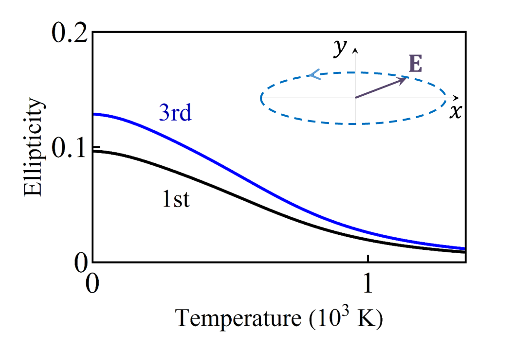
Figure 5: Circular birefrigence in graphene according to the hydrodynamic theory. The blue line is the ellipticity of the third-harmonic light ($|E_{y}/E_{x}|$) as a function of temperature at $n=10^{12}\,\mathrm{cm^{-2}}$. The black line is the ellipticity of the first-harmonic reflected light. The frequency is $\omega=1.41\,\mathrm{THz}$, the magnetic field is $B=0.1\,\mathrm{T}$. Inset: illustration of the elliptical polarization.

In the presence of an applied magnetic field, there is a finite second term $\propto\omega_{c}$ in Eq. (32), which causes the third-order circular birefringence. As in Sec. IV.3, let us consider a 2D system subject to a normally incident monochromatic light of frequency $\omega$ with the electric field polarized in the $x$-direction. The generated third-order current has frequency $\omega_{s}=3\omega$ and has a nonzero $y$-component

$$j_{x}(3\omega) =\sigma^{(3)}_{xxxx}E^{3}_{x}(\omega)=iD_{h}^{(3)}\frac{3}{\omega^{3}}\,,$$

$$j_{y}(3\omega) =\sigma^{(3)}_{yxxx}E^{3}_{x}(\omega)=iD_{h}^{(3)}\frac{3}{\omega^{3}}\left(\frac{4i\omega_{c}}{3\omega}\right)\,.$$ (42)

In the dissipationless limit, $\omega$ is real, and $j_{y}$ has a $\pi/2$ phase difference relative to $j_{x}$. Therefore, the third harmonic light will be elliptically polarized with the principal axis along $x$. Its ellipticity, conventionally denoted by $\tan\theta$, is given by

$$\tan\theta=\left|\frac{j_{y}}{j_{x}}\right|=\frac{4}{3}\frac{\omega_{c}}{\omega}\,.$$ (43)

Therefore, the ellipticity scales as $\omega_{c}=eB/m^{\ast}c$, which decays with temperature if the carrier density $n$ is fixed. This is illustrated by Fig. 5 for the case of graphene. From Eq. (26), there is also circular birefringence in the linear response, with $\tan\theta=\omega_{c}/\omega$, which differs only by the constant numerical factor $4/3$. It is also plotted in Fig. 5, for an easy comparison.

VIII Discussion

We showed that the third-order nonlinear conductivity $\sigma^{(3)}$ of a Dirac fluid has a universal functional form for any mass, chemical potential, temperature, and space dimension. It is remarkable that the third-order and the linear conductivities are simply related through Eqs. (5) and (31). Although we have used graphene as an example in the numerical calculations, our formulas, e.g., Eqs. (4) and (5), hold for any Lorentz-invariant Dirac fluid. As such, these formulas should be a good approximation to surface states of topological insulators and Dirac/Weyl semimetals, provided they are in the hydrodynamic regime. We also studied the field-induced renormalization of the dispersion of the collective modes (demons) and the third-order circular birefringence in the presence of a static magnetic field.

In the future it would be interesting to investigate hydrodynamics of non-Dirac fluids, that is, systems without the Lorentz symmetry. This will be important for more realistic modeling of ultrapure solid-state systems where hydrodynamic regime has been reported (GaAs, graphene, and $\mathrm{PdCoO_{2}}$). In the above systems, although the quasi particle band dispersion is approximately Dirac-like, the Coulomb interaction tends to break this quasi Lorentz symmetry because it propagates with the speed of light $c$ rather than $v$. It would also be interesting to study nonlinear thermal transport in the Dirac fluid. The case of phonon fluids has been studied half a century agoNielsen and Shklovskii (1969).

Appendix A Thermodynamic quantities in graphene

For convenience, below we list the expressions for the thermodynamic quantities of graphene in the noninteracting limit. The charge density $n(\mu,T)$ Sun et al. (2016) is

$$n =\int\limits_{-\infty}^{\infty}\left[f(\mu,T,\epsilon)-f(0,0,\epsilon)\right]g(\epsilon)d\epsilon=\frac{1}{\pi}\frac{\mu^{2}}{\hbar^{2}v_{F}^{2}}\Bigl{[}1+\frac{\pi^{2}}{3}\frac{T^{2}}{\mu^{2}}+4\,\frac{T^{2}}{\mu^{2}}\mathrm{Li}_{2}\bigl{(}-e^{-\mu/T}\bigl{)}\Bigr{]}\,$$ (44)

where $\mathrm{Li}_{s}(x)$ is the polylogarithm function. The energy density $n_{E}$ is defined relative to the $(\mu,T)=(0,0)$ case:

$$n_{E} =\int\limits_{-\infty}^{\infty}\left[f(\mu,T,\epsilon)-f(0,0,\epsilon)\right]\epsilon g(\epsilon)d\epsilon=\frac{2}{\pi}\frac{T^{3}}{\hbar^{2}v_{F}^{2}}\Bigl{[}\frac{\pi^{2}}{3}\,\frac{\mu}{T}+\frac{1}{3}\,\frac{\mu^{3}}{T^{3}}-4\,\mathrm{Li}_{3}\bigl{(}-e^{-\mu/T}\bigr{)}\Bigr{]}$$

$$=\frac{2}{3\pi}\frac{\mu^{3}}{\hbar^{2}v_{F}^{2}}\Bigl{[}1+\pi^{2}\frac{T^{2}}{\mu^{2}}-12\frac{T^{3}}{\mu^{3}}\mathrm{Li}_{3}\bigl{(}-e^{-\mu/T}\bigr{)}\Bigr{]}\,.$$ (45)

The enthalpy density is $W=\frac{3}{2}n_{E}$, the pressure is $P=\frac{1}{2}n_{E}$, and the entropy density is

$$s=\left(\frac{\partial P}{\partial T}\right)_{\mu}=\frac{1}{3\pi}\frac{\mu^{2}}{\hbar^{2}v_{F}^{2}}\Bigl{[}2\pi^{2}\frac{T}{\mu}-12\frac{T}{\mu}\mathrm{Li}_{2}\bigl{(}-e^{-\mu/T}\bigr{)}-36\frac{T^{2}}{\mu^{2}}\mathrm{Li}_{3}\bigl{(}-e^{-\mu/T}\bigr{)}\Bigr{]}\,.$$ (46)

The hydrodynamic effective mass $m^{\ast}(\mu,T)$ is

$$m^{\ast}(\mu,T)=\frac{1}{v^{2}}\frac{W(\mu,T)}{n(\mu,T)}\,.$$ (47)

The dimensionless bulk isentropic modulus is

$$C_{\mathrm{ise}}==\frac{1}{m^{\ast}\!v^{2}}\left(\frac{\partial P}{\partial n}\right)_{\mathrm{ise}}=\frac{1}{d}=\frac{1}{2}\,.$$ (48)

Appendix B Derivation of $\sigma^{(3)}$ with momentum and energy relaxation

In the homogeneous case, the hydrodynamic equations are

$$(\partial_{t}+\Gamma_{d})p_{i}=\rho E_{i},\quad\partial_{t}n_{E}=\rho\,u_{j}E_{j}-\Gamma_{E}\delta n_{E}-\Gamma_{k}Wu^{2},\,\quad\partial_{t}\rho=0\,,$$ (49)

where $\Gamma_{d}$ is the phenomenological momentum relaxation rate, $\Gamma_{E}$ can be called the cooling rate, $\delta n_{E}=n_{E}-n_{Eeq}$ is the fluctuation of energy density with respect to its steady-state value, and $\Gamma_{k}$ is the relaxation rate of the center-of-mass kinetic energy of a moving fluid. The last equation entails $\rho$ is constant. Therefore $j_{i}^{(3)}=\rho u^{(3)}_{i}$ and the momentum $p_{i}$ is strictly linear in electric field, same as the dissipationless case. The third-order velocity can be found from Eq. (20)

$$u_{i}^{(3)}=-\left(W^{(2)}/W+{u^{(1)}}^{2}\right)u_{i}^{(1)}\,.$$ (50)

By rotational symmetry, the leading order perturbation to the scalar quantities are second order in the electric field Sun et al.

$$\begin{split}n_{0}^{(2)}=-\frac{1}{2}n_{0}{u^{(1)}}^{2}\,,\quad n_{E}^{(2)}=\frac{\omega_{2}^{+}-i\Gamma_{k}}{\omega_{1}+\omega_{2}+i\Gamma_{E}}Wu^{(1)}_{1i}u^{(1)}_{2i}+\mathrm{perm}\,,\quad n_{E0}^{(2)}=n^{(2)}_{E}-W{u^{(1)}}^{2}\,.\end{split}$$ (51)

where “$\mathrm{perm}$” stands for permutations among subscripts $1$, $2$, and $3$, corresponding to frequencies $\omega_{1}$, $\omega_{2}$, and $\omega_{3}$, respectively. Note the difference between density $n_{0}$ and energy density $n_{E0}$ in proper frame and their counterparts $n$, $n_{E}$ in lab frame. With the second order expansion of the enthalpy

$$W^{(2)}=\left(\frac{\partial W}{\partial n_{0}}\right)_{n_{E0}}n_{0}^{(2)}+\left(\frac{\partial W}{\partial n_{E0}}\right)_{n_{0}}n_{E0}^{(2)}\,$$ (52)

we are ready to write down the third order flow velocity

$$u_{i}^{(3)}=-\left[\frac{1}{W}\left(\frac{\partial W}{\partial n_{0}}\right)_{n_{E0}}\left(-\frac{1}{2}n_{0}\right){u^{(1)}}^{2}+\left(\frac{\partial W}{\partial n_{E0}}\right)_{n_{0}}\left(\frac{\omega_{2}^{+}-i\Gamma_{k}}{\omega_{1}+\omega_{2}+i\Gamma_{E}}u^{(1)}_{1j}u^{(1)}_{2j}+\mathrm{perm}\right)-\left(\frac{\partial W}{\partial n_{E0}}\right)_{n_{0}}{u^{(1)}}^{2}+{u^{(1)}}^{2}\right]u_{i}^{(1)}\,.$$ (53)

where we defined $\omega_{a}^{+}\equiv\omega_{a}+i\Gamma_{d}$. The equation for the Fourier amplitude $u^{(3)}(\omega_{s})$ of the combined frequency $\omega_{s}=\omega_{1}+\omega_{2}+\omega_{3}$ becomes

$$u_{i}^{(3)} =-\left[\frac{1}{W}\left(\frac{\partial W}{\partial n_{0}}\right)_{n_{E0}}\left(-\frac{1}{2}n_{0}\right)+\left(\frac{\partial W}{\partial n_{E0}}\right)_{n_{0}}\left(\frac{\omega_{2}^{+}-i\Gamma_{k}}{\omega_{1}+\omega_{2}+i\Gamma_{E}}\right)-\left(\frac{\partial W}{\partial n_{E0}}\right)_{n_{0}}+1\right]u^{(1)}_{1j}u^{(1)}_{2j}u^{(1)}_{3i}+\mathrm{perm}$$

$$=\left[\frac{1}{2}\frac{n_{0}}{W}\left(\frac{\partial W}{\partial n_{0}}\right)_{n_{E0}}+\left(\frac{\partial W}{\partial n_{E0}}\right)_{n_{0}}-1-\frac{1}{2}\left(\frac{\partial W}{\partial n_{E0}}\right)_{n_{0}}\left(\frac{\omega_{1}^{+}+\omega_{2}^{+}-2i\Gamma_{k}}{\omega_{1}+\omega_{2}+i\Gamma_{E}}\right)\right]u^{(1)}_{1j}u^{(1)}_{2j}u^{(1)}_{3i}+\mathrm{perm}$$

$$=\frac{1}{2}\left[C_{\mathrm{ise}}-1-\left(\frac{\partial W}{\partial n_{E0}}\right)_{n_{0}}\left(\frac{2i\Gamma_{d}-i\Gamma_{E}-2i\Gamma_{k}}{\omega_{1}+\omega_{2}+i\Gamma_{E}}\right)\right]u^{(1)}_{1j}u^{(1)}_{2j}u^{(1)}_{3i}+\mathrm{perm}\,.$$ (54)

After the standard symmetrization procedure, Eq. (54) renders $\sigma^{(3)}$ with dissipation. The cooling rate $\Gamma_{E}$ could arise due to electron-phonon coupling and is crucial for eliminating the divergence of $\sigma^{(3)}$ in the dc limit. In this dc limit, due to work done by the electric field, the electron-hole fluid would be heated up by order $E^{2}/\Gamma_{E}$, thus inducing a large correction to the current at the third order. This is a physical reason why setting $\Gamma_{E}\to 0$ would lead to a diverging $\sigma^{(3)}$.

In the dissipationless limit, Eq. (54) becomes Eq. (23). Moreover, it can be readily checked that if $\Gamma_{E}+2\Gamma_{k}=2\Gamma_{d}$, Eq. (54) becomes identical to Eq. (23) as well. Under this condition, the fluid dynamics becomes isentropic again: the kinetic energy is lost to the environment due to momentum relaxation instead of converted into heat of the fluid.

Appendix C Relativistic Boltzmann equation

The relativistic Boltzmann equation is

$$\left(P^{\mu}\partial_{\mu}+F_{\mu\nu}P^{\mu}\partial_{P_{\nu}}\right)f_{R}(X,P)=I[f_{R}]\,,$$ (55)

where $f_{R}(X,P)$ is the relativistic distribution function and $I[f_{R}]$ is the collision integral due to interactions. Note that the space-time coordinate $X^{\mu}$ and the momentum $P^{\mu}=mu^{\mu}$ are covariant ones. For a given $X^{\mu}$, the distribution function $f_{R}(X,P)$ can be defined as the density of world lines whose local tangent is $P^{\mu}$. Mathematically, $f_{R}(X,P)$ is a scalar function defined on the tangent bundle of the $d+1$ dimensional space-time. If we focus on one species of particle with a fixed mass $m$, then $f_{R}(X,P)$ is related to the ordinary distribution function through

$$f_{R}(X,P)=f(t,\mathbf{r},\mathbf{p})\delta(E^{2}-p^{2}-m^{2})\,.$$ (56)

We integrate Eq. (55) over $P$ to get the charge continuity equation:

$$\partial_{\mu}J^{\mu}=0\,,$$

$$j^{\mu}=\int dPP^{\mu}f_{R}(X,P)=\int d\mathbf{p}\;(1,\mathbf{v})f(t,\mathbf{r},\mathbf{p})\,,$$ (57)

which is the second equation in Eq. (6).

Next, we multiply Eq. (55) by $P^{\alpha}$ and again integrate it over $P$. We get the continuity equation for the energy-momentum tensor,

$$\partial_{\mu}T^{\mu\nu}=F_{\mu}^{\nu}J^{\mu}\,,$$

$$T^{\mu\nu}=\int dPP^{\mu}P^{\nu}f_{R}(X,P)=\int d\mathbf{p}\;P^{\mu}P^{\nu}\frac{1}{E}f(t,\mathbf{r},\mathbf{p})\,,$$ (58)

which is the first equation in Eq. (6).

References

- Gurzhi (1968) R. N. Gurzhi, Sov. Phys. Uspekhi 11, 255 (1968).
- Andreev et al. (2011) A. V. Andreev, S. A. Kivelson, and B. Spivak, Phys. Rev. Lett. 106, 256804 (2011).
- Landau and Lifshitz (1987) L. D. Landau and E. M. Lifshitz, Fluid Mechanics, 2nd ed. (Pergamon Press, Oxford, 1987).
- de Jong and Molenkamp (1995) M. J. M. de Jong and L. W. Molenkamp, Phys. Rev. B 51, 13389 (1995).
- Bandurin et al. (2016) D. A. Bandurin, I. Torre, R. K. Kumar, M. Ben Shalom, A. Tomadin, A. Principi, G. H. Auton, E. Khestanova, K. S. Novoselov, I. V. Grigorieva, L. A. Ponomarenko, A. K. Geim, and M. Polini, Science 351, 1055 (2016).
- Crossno et al. (2016) J. Crossno, J. K. Shi, K. Wang, X. Liu, A. Harzheim, A. Lucas, S. Sachdev, P. Kim, T. Taniguchi, K. Watanabe, T. A. Ohki, and K. C. Fong, Science 351, 1058 (2016).
- Krishna Kumar et al. (2017) R. Krishna Kumar, D. A. Bandurin, F. M. D. Pellegrino, Y. Cao, A. Principi, H. Guo, G. H. Auton, M. Ben Shalom, L. A. Ponomarenko, G. Falkovich, K. Watanabe, T. Taniguchi, I. V. Grigorieva, L. S. Levitov, M. Polini, and A. K. Geim, Nat. Phys. (2017), 10.1038/nphys4240.
- Moll et al. (2016) P. J. W. Moll, P. Kushwaha, N. Nandi, B. Schmidt, and A. P. Mackenzie, Science 351, 1061 (2016).
- Müller et al. (2008) M. Müller, L. Fritz, and S. Sachdev, Phys. Rev. B 78, 115406 (2008).
- Müller et al. (2009) M. Müller, J. Schmalian, and L. Fritz, Phys. Rev. Lett. 103, 025301 (2009).
- (11) T. V. Phan, J. C. W. Song, and L. S. Levitov, “Ballistic Heat Transfer and Energy Waves in an Electron System,” (unpublished), arXiv:1306.4972 .
- Forcella et al. (2014) D. Forcella, J. Zaanen, D. Valentinis, and D. van der Marel, Phys. Rev. B 90, 035143 (2014).
- Briskot et al. (2015) U. Briskot, M. Schütt, I. V. Gornyi, M. Titov, B. N. Narozhny, and A. D. Mirlin, Phys. Rev. B 92, 115426 (2015).
- Narozhny et al. (2015) B. N. Narozhny, I. V. Gornyi, M. Titov, M. Schütt, and A. D. Mirlin, Phys. Rev. B 91, 035414 (2015).
- Principi and Vignale (2015a) A. Principi and G. Vignale, Phys. Rev. B 91, 205423 (2015a).
- Principi and Vignale (2015b) A. Principi and G. Vignale, Phys. Rev. Lett. 115, 056603 (2015b).
- Sun et al. (2016) Z. Sun, D. N. Basov, and M. M. Fogler, Phys. Rev. Lett. 117, 076805 (2016).
- Lucas et al. (2016) A. Lucas, J. Crossno, K. C. Fong, P. Kim, and S. Sachdev, Phys. Rev. B 93, 075426 (2016).
- Lucas (2017) A. Lucas, Phys. Rev. B 95, 115425 (2017).
- (20) Z. Sun, D. N. Basov, and M. M. Fogler, (unpublished), arXiv:1704.07334 .
- Guo et al. (2017) H. Guo, E. Ilseven, G. Falkovich, and L. S. Levitov, Proc. Natl. Acad. Sci. 114, 3068 (2017).
- Mikhailov (2007) S. A. Mikhailov, Europhys. Lett. 79, 27002 (2007).
- Mikhailov (2011) S. A. Mikhailov, Phys. Rev. B 84, 045432 (2011).
- Gullans et al. (2013) M. Gullans, D. E. Chang, F. H. L. Koppens, F. J. G. de Abajo, and M. D. Lukin, Phys. Rev. Lett. 111, 247401 (2013).
- Cheng et al. (2014) J. L. Cheng, N. Vermeulen, and J. E. Sipe, New J. Phys. 16, 053014 (2014).
- Yao et al. (2014) X. Yao, M. Tokman, and A. Belyanin, Phys. Rev. Lett. 112, 055501 (2014).
- Cheng et al. (2015) J. L. Cheng, N. Vermeulen, and J. E. Sipe, Phys. Rev. B 91, 235320 (2015).
- Mikhailov (2016) S. A. Mikhailov, Phys. Rev. B 93, 085403 (2016).
- Tokman et al. (2016) M. Tokman, Y. Wang, I. Oladyshkin, A. R. Kutayiah, and A. Belyanin, Phys. Rev. B 93, 235422 (2016).
- Cheng et al. (2017) J. L. Cheng, N. Vermeulen, and J. E. Sipe, Sci. Rep. 7, 43843 (2017).
- (31) M. T. Manzoni, I. Silveiro, F. J. G. D. Abajo, and D. E. Chang, New J. Phys. 17, 83031.
- Wang et al. (2016) Y. Wang, M. Tokman, and A. Belyanin, Phys. Rev. B 94, 195442 (2016).
- Rostami et al. (2017) H. Rostami, M. I. Katsnelson, and M. Polini, Phys. Rev. B 95, 035416 (2017).
- Ni et al. (2016) G. X. Ni, L. Wang, M. D. Goldflam, M. Wagner, Z. Fei, A. S. McLeod, M. K. Liu, F. Keilmann, B. Özyilmaz, A. H. Castro Neto, J. Hone, M. M. Fogler, and D. N. Basov, Nature Photon. 10, 244 (2016).
- Son et al. (2018) S.-k. Son, M. Šiškins, C. Mullan, J. Yin, V. G. Kravets, A. Kozikov, S. Ozdemir, M. Alhazmi, M. Holwill, K. Watanabe, T. Taniguchi, D. Ghazaryan, K. S. Novoselov, V. I. Fal’ko, and A. Mishchenko, 2D Materials 5, 011006 (2018).
- Giorgianni et al. (2016) F. Giorgianni, E. Chiadroni, A. Rovere, M. Cestelli-Guidi, A. Perucchi, M. Bellaveglia, M. Castellano, D. Di Giovenale, G. Di Pirro, M. Ferrario, R. Pompili, C. Vaccarezza, F. Villa, A. Cianchi, A. Mostacci, M. Petrarca, M. Brahlek, N. Koirala, S. Oh, and S. Lupi, Nat. Commun. 7, 11421 (2016).
- Landau and Lifshitz (1984) L. D. Landau and E. M. Lifshitz, Electrodynamics of Continuous Media (Pergamon, Oxford, 1984).
- Boyd (2008) R. W. Boyd, Nonlinear optics, 3rd ed. (Academic Press, 2008).
- Mikhailov (2017) S. A. Mikhailov, ACS Photonics (2017), 10.1021/acsphotonics.7b00468.
- Nielsen and Shklovskii (1969) H. Nielsen and B. I. Shklovskii, Sov. Phys. JETP 56, 709 (1969).