Optimal Global Test for Functional Regression

Simeng Qu and Xiao Wang

Department of Statistics, Purdue University

Abstract: This paper studies the optimal testing for the nullity of the slope function in the functional linear model using smoothing splines. We propose a generalized likelihood ratio test based on an easily implementable data-driven estimate. The quality of the test is measured by the minimal distance between the null and the alternative set that still allows a possible test. The lower bound of the minimax decay rate of this distance is derived, and test with a distance that decays faster than the lower bound would be impossible. We show that the minimax optimal rate is jointly determined by the smoothing spline kernel and the covariance kernel. It is shown that our test attains this optimal rate. Simulations are carried out to confirm the finite-sample performance of our test as well as to illustrate the theoretical results. Finally, we apply our test to study the effect of the trajectories of oxides of nitrogen ($\text{NO}_{\text{x}}$) on the level of ozone ($\text{O}_{3}$).

Key words and phrases: Functional linear model, generalized likelihood ratio test, minimax rate of convergence, reproducing kernel, smoothing splines.

1 Introduction

Functional linear regression model, with respect to nonparametric estimation and prediction, has drawn extensive attention in the field of functional data analysis in recent years. The model is stated as

$$Y=a_{0}+\int_{0}^{1}\beta_{0}(t)X(t)dt+\epsilon,$$ (1)

where $Y$ is a scalar response, $X:[0,1]\rightarrow\mathbb{R}$ is a square integrable random functional predictor, $\alpha_{0}\in\mathbb{R}$ is the intercept, $\beta_{0}:[0,1]\rightarrow\mathbb{R}$ is the slope function, and $\epsilon$ is the random error with mean zero and variance $\sigma^{2}$. One of the popular methods to study such model is based on the functional principal component analysis (James, 2002; Ramsay and Silverman, 2005; Yao et al., 2005b; Cai and Hall, 2006; Li and Hsing, 2007; Hall and Horowitz, 2007). In addition, regularization method has also been applied to study the model (Crambes et al., 2009; Yuan and Cai, 2010; Cai and Yuan, 2012; Du and Wang, 2014; Wang and Ruppert, 2015). Although the asymptotic properties of estimators of $\beta_{0}$ are widely discussed in the literature, there is little research on testing whether $\beta_{0}$ resides in a given finite dimensional linear subspace, or more specifically, $\beta_{0}\equiv 0$.

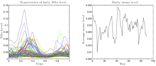
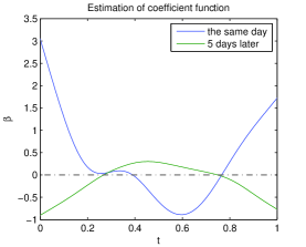
Figure 1: Left: the daily trajectories of $\text{NO}_{\text{x}}$ levels. Middle: average $\text{O}_{3}$ level each day. Right: estimated coefficient functions

Take the study of California air quality data as an example.Effects of oxides of nitrogen ($\text{NO}_{\text{x}}$) on levels of ozone ($\text{O}_{3}$) is always of great interest to meteorology researchers. The left and middle panels of Figure 1 displays the daily trajectories of $\text{NO}_{\text{x}}$ levels as well as the daily average $\text{O}_{3}$ levels in the city of Sacramento from June 1 to August 31 in 2005. If we take daily $\text{NO}_{\text{x}}$ trajectory as predictor $X(t)$ and average $\text{O}_{3}$ level as $Y$, then an absent effect will be indicated by a zero slope function in model (2). The right panel of Figure 1 plots the estimated slope functions under two settings, (1) response $Y$ is the $\text{O}_{3}$ level of the same day as $\text{NO}_{\text{x}}$ trajectory, and (2) response is the $\text{O}_{3}$ level five days later after the recorded $\text{NO}_{\text{x}}$ trajectory. Under setting (1), the estimated slope function has a large magnitude and a clear curve. This indicates that the true slope function in this model is very unlikely to be a zero function, that is to say, a day’s $\text{NO}_{\text{x}}$ has a strong effect on its $\text{O}_{3}$ level. On the other hand, the estimated slope function under setting (2) stays close to zero and the slight curvature of this estimated slope function may due to randomness of the data, with the true $\beta_{0}$ residing in a zero null space. In other words, a day’s $\text{NO}_{\text{x}}$ may barely have any effect on the $\text{O}_{3}$ level five days later. However to draw a statistical conclusion under a certain significant level on whether there is still some effect on the $\text{O}_{3}$ level from the $\text{NO}_{\text{x}}$ level five days ago, we need a well-designed testing procedure.

Cardot et al. (2003) proposed a test statistic based on the first $k$ functional components of $X$. However, selection of $k$ is a difficult problem. Some computational methods have been proposed to resolve this issue without theoretical guarantee on the power (Cardot et al., 2004; González-Manteiga and Martínez-Calvo, 2011). For more recent work, Hilgert et al. (2013) used the functional principle component approach to test the nullity of the slope function, and established that their procedures are minimax adaptive to the unknown regularity of the slope. In particular, they assumed that $\beta_{0}\in{\cal E}_{a}(L)$ where

$${\cal E}_{a}(L)=\Big{\{}\beta\in L_{2}[0,1]:\sum_{k=1}^{\infty}a_{k}^{-2}\big{\langle}\beta,\varphi_{k}\big{\rangle}^{2}\leq L^{2}\Big{\}},$$

with $\langle\beta,\varphi_{k}\rangle=\int_{0}^{1}\beta(t)\varphi_{k}(t)dt$, and $\varphi_{k}$’s are eigenfunctions of the covariance $\Gamma$. The smoothness of $\beta_{0}$ is characterized by the decay rate of $a_{k}$. ${\cal E}_{a}(L)$ is essentially a reproducing kernel Hilbert space (RKHS), denoted by ${\cal H}(K)$, with a specific reproducing kernel $K(t,s)=\sum_{k=1}^{\infty}a_{k}^{2}\varphi_{k}(t)\varphi_{k}(s)$. When their underline assumption that, kernel $K$ and $\Gamma$ are well aligned, is not satisfied, their methods may not perform well. Lei (2014) developed a method simultaneously testing the slope vectors in a sequence of functional principal components regression models, and showed that under certain conditions, his method is uniformly powerful over a class of smooth alternatives. However, the principal-component-based methods are successful upon the assumption that the slope function $\beta(t)$ can be well represented by the leading functional principal components of $X$. Cai and Yuan (2012) showed that, for the benchmark Canadian weather data, the estimated Fourier coefficients of the slope function with respect to the eigenfunctions of the sample covariance function do not decay at all, which is a typical example for the case that the slope function is not well represented by the leading principal components. Shang and Cheng (2015) proposed a roughness regularization approach in making non-parametric inference for generalized functional linear model, including a theoretical result on the upper bound.

In this paper, we propose an adaptive and minimax optimal testing procedures on detecting the nullity of the slope function in functional linear model using smoothing splines. Let $\Gamma(s,t)$ denote the covariance function of $X$. $\Gamma$ can also be taken as a nonnegative definite operator with $\Gamma f=\int_{0}^{1}\Gamma(\cdot,~{}t)f(t)dt$ for $f\in L_{2}$. We wish to test the null hypothesis $H_{0}:\beta\equiv 0$ against the composite nonparametric alternative that $\beta_{0}$ is separated away from zero in terms of a $L_{2}$-norm induced by the operator $\Gamma$, i.e. $\|\beta_{0}\|_{\Gamma}\geq\varrho_{n}$, where $\|\beta\|_{\Gamma}^{2}=\langle\Gamma\beta,\beta\rangle$ with $\langle\beta,\gamma\rangle=\int_{0}^{1}\beta(t)\gamma(t)dt$. Then assuming that the unknown slope function $\beta_{0}$ possesses some smoothness properties, therefore, we arrive at the following alternative: $H_{1}:{\cal F}_{\Gamma}(\rho_{n})=\{\beta:\|\beta\|_{\Gamma}\geq\rho_{n}\}$. The radius $\rho_{n}$ characterizes the sensitivity of the test. We investigate the optimal decay rate of the radius $\rho_{n}$, under which the test with prescribed probabilities of errors is still possible.

The paper is organized as follows. In Section 2, a smoothing spline estimate for the slope function is introduced, and a generalized likelihood ratio test based on this smoothing spline estimate is proposed. In Section 3, we show that our test is optimal in the sense that it achieves the minimax lower bound, which is joint determined by the smoothing spline kernel and the covariance kernel. Section 4 demonstrates the finite sample performance of the test under different simulated setups. Later in this section come more details about the air quality example.

2 Generalized Likelihood Ratio Test

2.1 Notation and definitions

Since our main focus is on the coefficient function $\beta(t)$, we assume both $X$ and $Y$ are centered, i.e., $E(Y)=0$ and $E(X(t))=0$ for all $t$. Therefore by taking expectation over both sides of (1), we have $\alpha_{0}=0$. Let $(X_{i},Y_{i}),i=1,\ldots,n$ be independent and identically distributed observations sampled from the model. Then model (1) can be rewritten as

$$Y_{i}=\int_{0}^{1}\beta_{0}(t)X_{i}(t)dt+\epsilon_{i},~{}~{}~{}~{}i=1,\ldots,n.$$ (2)

$\beta_{0}(t)$ is considered to reside in the Sobolev space $W_{2}^{m}$ of order $m$, defined as

$$W_{2}^{m}=\Big{\{}\beta:[0,1]\rightarrow\mathbb{R}\Big{|}\beta,\beta^{\prime},\ldots,\beta^{(m-1)}\text{ are absolutely continuous and }\beta^{(m)}\in L_{2}[0,1]\Big{\}}.$$

Equipting $W_{2}^{m}$ with a reproducing kernel

$$K(t,s)=\sum_{k=0}^{m-1}\frac{s^{k}t^{k}}{(k!)^{2}}+R(t,s),\quad\text{where }R(t,s)=\int_{0}^{1}\frac{(s-u)_{+}^{m-1}(t-u)_{+}^{m-1}}{\{(m-1)!\}^{2}}du,$$

it becomes a reproducing kernel Hilbert space (Wahba, 1990), denoted as ${\cal H}(K)$.

Let $T_{0}$ and $T_{1}$ be operators on $L_{2}[0,1]$ such that

$$T_{0}X(t)=\int_{0}^{t}X(s)ds~{}~{}~{}~{}~{}\mbox{and}~{}~{}~{}~{}~{}T_{1}X(t)=\int_{t}^{1}X(s)ds.$$

It follows Fubini’s theorem that $\langle f,T_{0}g\rangle=\langle T_{1}f,g\rangle$, and thus $T_{0}$ is the adjoint operator to $T_{1}$. Further, define that $T_{0}^{k}X(t)=T_{0}T_{0}^{k-1}X(t)$ and $T_{1}^{k}X(t)=T_{1}T_{1}^{k-1}X(t)$ for $k\geq 2$. Therefore, $T_{0}^{k}$ is the adjoint operator to $T_{1}^{k}$, and

$$T_{0}^{k}X(t)=\int_{0}^{1}\frac{(t-s)_{+}^{k-1}}{(k-1)!}X(s)ds,~{}~{}~{}~{}~{}T_{1}^{k}X(t)=\int_{0}^{1}\frac{(s-t)_{+}^{k-1}}{(k-1)!}X(s)ds.$$

In particular,

$$R=T_{0}^{m}T_{1}^{m}.$$

Observe that $R$ differs from $K$ only by a polynomial of degree less than or equal to $m$. Therefore, their eigenvalues have the same decay rate.

The following notations will be used in estimating slope function and then constructing test statistic. Denote ${\bf X}(t)=(X_{1}(t),\ldots,X_{n}(t))^{T}$ and sample covariance function $\hat{\Gamma}(t,s)=n^{-1}{\bf X}(t)^{T}{\bf X}(s)$. Let $\widetilde{X}(1)\in\mathbb{R}^{m\times n}$ be an $m$ by $n$ matrix with the $(i,j)^{\prime}s$ element $(\widetilde{X}(1))_{i,j}=T_{0}^{i}X_{j}(1)$ and $\hat{H}=n^{-1}\widetilde{X}(1)\widetilde{X}(1)^{T}$. Define a matrix $\hat{B}=\frac{1}{n}\widetilde{X}(1)^{T}\hat{H}^{-1}\widetilde{X}(1)$, then $\hat{B}$ is an $n\times n$ idempotent matrix with $\hat{B}^{2}=\hat{B}$. Finally, define an operator $\hat{Q}$ as $\hat{Q}(t,s)=n^{-1}\hat{U}(t)^{T}\hat{U}(s)$, where $\hat{U}(t)$ is a random function vector such that

$$\hat{U}(t)=(I_{n}-\hat{B})T_{0}^{m}{\bf X}(t).$$

It is easy to see that

$$\hat{Q}=n^{-1}T_{0}^{m}{\bf X}^{T}(I_{n}-\hat{B})T_{0}^{m}{\bf X}=T_{0}^{m}\big{(}\hat{\Gamma}-\hat{\Gamma}_{0}\big{)}T_{1}^{m},$$

where

$$\hat{\Gamma}_{0}(t,s)=\frac{1}{n}{\bf X}(t)^{T}B{\bf X}(s),$$

is a degenerated operator with at most $m$ eigenvalues. Hence, the eigenvalues of $\hat{Q}$, $T_{0}^{m}\hat{\Gamma}T_{1}^{m}$ and further $T\Gamma T^{*}$ have the same decay rate.

2.2 The smoothing spline estimator

In this section, we study the smoothing spline estimate which will be used to construct the generalized likelihood ratio test in the next session. Let $\hat{\beta}$ be the smoothing spline estimate such that $\hat{\beta}\in W_{2}^{m}$ minimizes

$$\frac{1}{n}\sum_{i=1}^{n}\Big{\{}Y_{i}-\int_{0}^{1}\beta(t)X_{i}(t)dt\Big{\}}^{2}+\lambda\int_{0}^{1}\Big{\{}\beta^{(m)}(s)\Big{\}}^{2}ds,$$ (3)

where $\lambda>0$ is the smoothing parameter. Next theorem provides the characterization of $\hat{\beta}$.

Theorem 1.

Denote ${\bf Y}=(Y_{1},\ldots,Y_{n})^{T}$ and operator $\hat{Q}^{+}=(\lambda I+\hat{Q})^{-1}$.

(a). The $m$th derivative of $\hat{\beta}$ is

$$\hat{\beta}^{(m)}=(-1)^{m}\frac{1}{n}\hat{Q}^{+}\hat{U}^{T}{\bf Y}.$$

(b). Let $\widehat{\Upsilon}(1)=\Big{[}\hat{\beta}(1),-\hat{\beta}^{\prime}(1),\ldots,(-1)^{m-1}\hat{\beta}^{(m-1)}(1)\Big{]}^{T}$. We have

$$\widehat{\Upsilon}(1)=\frac{1}{n}\hat{H}^{-1}\widetilde{X}(1)\Big{\{}I_{n}-\frac{1}{n}\int_{0}^{1}T_{0}^{m}{\bf X}(s)~{}\hat{Q}^{+}\hat{U}(s)^{T}ds\Big{\}}{\bf Y}.$$

Theorem 1 provides a brand new approach to compute $\hat{\beta}$ explicitly over the infinitely dimensional function space ${\cal H}(K)$. This observation is important to both numerical implementation and asymptotic analysis. The explicit formula for $\hat{\beta}$ is

$$\hat{\beta}(t)=\widehat{\Upsilon}(1)^{T}\zeta(t)+(-1)^{m}\int_{0}^{1}\hat{\beta}^{(m)}(s)\frac{(s-t)_{+}^{m-1}}{(m-1)!}ds=\Pi_{t}{\bf Y}$$ (4)

where $\zeta(t)=\Big{[}1,(1-t),\frac{(1-t)^{2}}{2!},\ldots,\frac{(1-t)^{m-1}}{(m-1)!}\Big{]}^{T}$, and

$$\Pi_{t}=\frac{1}{n}\zeta(t)^{T}\hat{H}^{-1}\widetilde{X}(1)\Big{\{}I_{n}-\frac{1}{n}\int_{0}^{1}T_{0}^{m}{\bf X}(s)~{}\hat{Q}^{+}\hat{U}(s)^{T}ds\Big{\}}+\frac{1}{n}T_{1}^{m}\hat{Q}^{+}\hat{U}(t)^{T}.$$

Therefore, $\hat{\beta}$ is a linear function of the response ${\bf Y}$ with $\Pi_{t}$ as the hat matrix.

2.3 Generalized likelihood ratio test

Assuming that $\epsilon_{i}$ follows normal distribution, the conditional log-likelihood function for (2) becomes

$$\ell_{n}(\beta,\sigma)=-n\log(\sqrt{2\pi}~{}\sigma)-\frac{1}{2\sigma^{2}}\sum_{i=1}^{n}\Big{(}Y_{i}-\int\beta X_{i}\Big{)}^{2}.$$

Define the residual sum of squares under the null and alternative hypothesis as follows:

$$\mbox{RSS}_{0}=\sum_{i=1}^{n}Y_{i}^{2},~{}~{}~{}\mbox{RSS}_{1}=\sum_{i=1}^{n}(Y_{i}-\int\hat{\beta}X_{i})^{2}.$$

Then the logarithm of the conditional maximum likelihood ratio test statistic is given by

$$\tau_{n,\lambda}=\ell_{n}(\hat{\beta},\hat{\sigma}_{1})-\ell_{n}(0,\hat{\sigma}_{0})=\frac{n}{2}\log\frac{\mbox{RSS}_{0}}{\mbox{RSS}_{1}},$$ (5)

where $\hat{\sigma}_{1}^{2}=\mbox{RSS}_{1}/n$ and $\hat{\sigma}_{0}^{2}=\mbox{RSS}_{0}/n$. Define an $n\times n$ matrix $A_{n}=A_{n}(\boldsymbol{X})$ as

$$A_{n}=\frac{1}{n}\int_{0}^{1}\hat{U}(t)\hat{Q}^{+}\hat{U}(t)^{T}dt-\frac{1}{2n}\int_{0}^{1}\int_{0}^{1}\hat{Q}^{+}\hat{U}(t)\hat{Q}(t,s)\hat{Q}^{+}\hat{U}(s)^{T}dtds+\frac{1}{2}\hat{B}.$$

Next theorem shows the properties of the test statistic $\tau_{n,\lambda}$.

Theorem 2.

. If $tr(A_{n})=o_{p}(n)$, we have the following results,

(a). Under $H_{0}:\beta\equiv 0$, the likelihood ratio test statistic $\tau_{n,\lambda}$ is of the form

$$\tau_{n,\lambda}=z^{T}A_{n}z+o_{p}\big{(}1\big{)},$$

where $z=\epsilon/\sigma$. Furthermore,let $\mu_{n}=tr(A_{n})$ and $\sigma_{n}^{2}=2\,tr(A_{n}^{2})$. If $\epsilon_{i}$, $i=1,...,n$ are independent and identically distributed following $\mathcal{N}(0,\sigma^{2})$, then $(\tau_{n,\lambda}-\mu_{n})/\sigma_{n}$has an asymptotic standard normal distribution.

(b). Under $H^{\prime}_{1}:{\cal F}^{\prime}_{K,\Gamma}(\rho_{n})=\Big{\{}\beta\in{\cal H}(K):\|\beta\|_{\Gamma}=\rho_{n}\Big{\}},$ if $\rho_{n}^{2}=o(n^{-1/2})$ and $\lambda=o(n^{-1/2})$, then

$$\tau_{n,\lambda}=z^{T}A_{n}z+\frac{n}{2\sigma^{2}}\|\beta_{0}\|_{\hat{\Gamma}}^{2}+O_{p}\Big{(}n\lambda+n^{1/2}\lambda^{1/2}+n^{1/2}\|\beta_{0}\|_{\hat{\Gamma}}\Big{)}.$$

The condition that $tr(A_{n})=o_{p}(n)$ in Theorem 2 can be satisfied in many cases. In fact, $tr(A_{n})$ can be computed explicitly. Consider the spectral decomposition of operator $\hat{Q}$, $\hat{Q}(t,s)=\sum_{j=1}^{\infty}\hat{\kappa}_{j}\hat{\phi}_{j}(t)\hat{\phi}_{j}(s)$, where $(\hat{\kappa}_{j},\hat{\phi}_{j})$ are (eigenvalue, eigenfunction) pairs, ordered such that $\hat{\kappa}_{1}\geq\hat{\kappa}_{2}\geq\cdots\geq 0$. We may write $\hat{U}_{X_{i}}(t)=\sum_{k=1}^{\infty}\hat{\xi}_{ik}\hat{\phi}_{k}(t)$. Since $\hat{Q}(t,s)=n^{-1}\sum_{i=1}^{n}\hat{U}_{X_{i}}(t)\hat{U}_{X_{i}}(s)$, we have $n^{-1}\sum_{i=1}^{n}\hat{\xi}_{ik}^{2}=\hat{\kappa}_{k}$ and $n^{-1}\sum_{i=1}^{n}\hat{\xi}_{ik}\hat{\xi}_{ij}=0$ for $k\neq j$. It is not hard to obtain that

$$tr(A_{n})=\sum_{k=1}^{\infty}\frac{\hat{\kappa}_{k}(\lambda+\frac{1}{2}\hat{\kappa}_{k})}{(\lambda+\hat{\kappa}_{k})^{2}}+\frac{m}{2}.$$

Furthermore, Lemma 3 shows that $tr(A_{n})=O_{p}(\sum_{k=1}^{\infty}\frac{s_{k}}{\lambda+s_{k}})$, which is determined by the order of $\lambda$ and the decay rate of $s_{k}$, the sorted eigenvalues of linear operator $T\Gamma T^{*}$. More specifically, if $s_{k}$ has a polynomial decay rate as $s_{k}\asymp k^{-2r}$, for some $r>1/2$, then $tr(A_{n})=O_{p}(\lambda^{-1/2r})$, while if $s_{k}$ has an exponential decay rate as $s_{k}\asymp e^{-2rk}$ for some $r>0$, then $tr(A_{n})=O(\log\mbox{$\lambda$}^{-1})$. In both cases, $tr(A_{n})=o_{p}(n)$ will be satisfied once we choose a proper $\lambda$. The optimal order of $\lambda$ will be shown later in Theorem 4, followed by a data-driven procedure of choosing $\lambda$.

Based on Theorem 2, we have an $\alpha$ level testing procedure that, we reject $H_{0}$ when $\frac{\tau_{n,\lambda}-\mu_{n}}{\sigma_{n}}>z_{\alpha}$ where $z_{\alpha}$ is the upper $\alpha$ quantile of the standard normal distribution. In the next section, we will show that the power function of this test is asymptotically one at the minmax optimal rate.

3 Optimal Test

3.1 Minimax lower bound

Let $\phi_{n}$ be a measurable function of the observations taking values at two points $\{0,1\}$. We accept $H_{0}$ if $\phi_{n}=0$, and reject $H_{0}$ if $\phi_{n}=1$. The probability of type I error, denoted by $\alpha_{0}(\phi_{n})$, is

$$\alpha_{0}(\phi_{n})=\mathbb{P}_{0}(\phi_{n}=1),$$

where $\mathbb{P}_{0}$ is the probability measure on the space of observations corresponding to $H_{0}$. The probability of type II error, denoted by $\alpha_{1}(\phi_{n})$, is

$$\alpha_{1}(\phi_{n},\rho_{n})=\sup_{\beta\in{\cal F}_{K,\Gamma}(\rho_{n})}\mathbb{P}_{\beta}(\phi_{n}=0),$$

where $\mathbb{P}_{\beta}$ is the probability measure corresponding to a particular slope function $\beta$. Let

$$\gamma_{n}(\phi_{n},\rho_{n})=\alpha_{0}(\phi_{n})+\alpha_{1}(\phi_{n},\rho_{n}),$$

which measures the error of the test $\phi_{n}$ by summarizing probability of the type I and type II errors. Fix a number $0<\gamma<1$. A sequence $\rho_{n}\rightarrow 0$ as $n\rightarrow\infty$ is called the minimax rate of testing if:

(i)

For any sequence $\rho^{\prime}_{n}$ such that $\rho^{\prime}_{n}/\rho_{n}\rightarrow 0$, we have $\lim\inf_{n\rightarrow\infty}\inf_{\phi_{n}}\gamma_{n}(\phi_{n},\rho_{n}^{\prime})\geq\gamma$;

(ii)

There exists a test $\phi_{n}^{*}$ such that $\lim\sup_{n\rightarrow\infty}\gamma_{n}(\phi_{n}^{*},\rho_{n})\leq\gamma$.

For the given reproducing kernel $K$, let $T$ and $T^{*}$ be two operators acting on $L_{2}[0,1]$ such that $K=TT^{*}$, where $T^{*}$ is the adjoint operator to $T$ with $\langle f,Tg\rangle=\langle T^{*}f,g\rangle$. Consider the linear operator $T\Gamma T^{*}$. It follows from the spectral theorem that

$$T\Gamma T^{*}(t,s)=\sum_{k=1}^{\infty}s_{k}\varphi_{k}(t)\varphi_{k}(s),$$

where $s_{1}\geq s_{2}\geq\cdots>0$ are the eigenvalues of the operator $T\Gamma T^{*}$ and $\varphi_{k}$’s are the corresponding eigenfunctions. For any two sequences $a_{k},b_{k}>0$, $a_{k}\asymp b_{k}$ means that $a_{k}/b_{k}$ is bounded away from zero and infinity as $k\rightarrow\infty$.

Theorem 3.

Assume $\epsilon_{i}$, $i=1,...,n$ are independent and identically distributed following $\mathcal{N}(0,\sigma^{2})$. Let $\{s_{k}:k\geq 1\}$ be the sorted eigenvalues of the linear operator $T\Gamma T^{*}$.

(a). When $s_{k}\asymp k^{-2r}$ for some constant $r>1/2$, let

$$\rho_{n}=n^{-2r/(1+4r)}.$$ (6)

If $\rho_{n}^{\prime}$ is such that $\rho_{n}^{\prime}/\rho_{n}\rightarrow 0$ as $n\rightarrow\infty$, then

$$\liminf_{n\rightarrow\infty}\inf_{\phi_{n}}\gamma_{n}(\phi_{n},\rho_{n}^{\prime})\geq 1.$$

(b). When $s_{k}\asymp e^{-2rk}$ for some constant $r>0$, let

$$\rho_{n}=\Big{(}\frac{\log n}{2rn^{2}}\Big{)}^{1/4}.$$ (7)

If $\rho_{n}^{\prime}$ is such that $\rho_{n}^{\prime}/\rho_{n}\rightarrow 0$ as $n\rightarrow\infty$, then

$$\liminf_{n\rightarrow\infty}\inf_{\phi_{n}}\gamma_{n}(\phi_{n},\rho_{n}^{\prime})\geq 1.$$

The cholesky decomposition of the operator $K=TT^{*}$ is not unique, and $T$ is not necessarily a symmetric operator. If we would like $T$ to be a symmetric operator, we may choose $T=T^{*}=K^{1/2}$. It is shown in the next proposition that the decay rate of the eigenvalues of the operator $T\Gamma T^{*}$ and $K^{1/2}\Gamma K^{1/2}$ have the same asymptotic order.

Proposition 1.

Let $K=TT^{*}$, where $T^{*}$ is adjoint to $T$. The eigenvalues of the two operators $T\Gamma T^{*}$ and $K^{1/2}\Gamma K^{1/2}$ have the same decay rate.

The minimax lower bound for the excess prediction risk has been established by Cai and Yuan (2012). Suppose the $kth$ eigenvalues of the linear operator $K^{1/2}\Gamma K^{1/2}$ is of order $k^{-2r}$ for some constant $0<r<\infty$, then

$$\lim_{a\rightarrow 0}\lim_{n\rightarrow\infty}\inf_{\hat{\beta}}\sup_{\beta_{0}\in H(K)}\mathbb{P}\Big{(}\big{\|}\hat{\beta}-\beta_{0}\big{\|}_{\Gamma}\geq an^{-\frac{r}{2r+1}}\Big{)}=1.$$

It turns out that the optimal separating rate $\rho_{n}$ for testing differs from the optimal rate for the problem of prediction. Similar situation arises in the setting of nonparametric regression.

Consider a special case that the reproducing kernel $K$ is perfectly aligned with $\Gamma$, i.e., $K(s,t)=\sum_{k=1}^{\infty}a_{k}^{2}\psi_{k}(t)\psi_{k}(s)$ and $\Gamma(t,s)=\sum_{k=1}^{\infty}\eta_{k}\psi_{k}(t)\psi_{k}(s)$. In this case, it is easy to see that $K^{1/2}\Gamma K^{1/2}(t,s)=\sum_{k=1}^{\infty}\eta_{k}a_{k}^{2}\psi_{k}(t)\psi_{k}(s)$, which indicates that $s_{k}=\eta_{k}a_{k}^{2}$. This special case has been studied in Hilgert et al. (2013).

3.2 Optimal adaptive test

Now back to the generalized likelihood ratio test. Recall that the test statistic $\tau_{n,\lambda}$ has an asymptotic normal distribution with mean $\mu_{n}=tr(A_{n})$ and variance $\sigma_{n}^{2}=2\,tr(A_{n}^{2})$. Concerning the distribution of the random function $X$, we shall assume that

(A1).

$X$ has a finite fourth moment, i.e., $\int_{0}^{1}E(X^{4})<\infty$ and

$$E\Big{(}\big{\langle}X,\psi_{k}\big{\rangle}^{4}\Big{)}\leq C\Big{(}E\big{\langle}X,\psi_{k}\big{\rangle}^{2}\Big{)}^{2}~{}~{}~{}~{}\mbox{for }k\geq 1,$$

where $C>0$ is a constant and $\psi_{k}$’s are eigenfunctions of $\Gamma$.

Theorem 4.

Assume (A1) holds and $\epsilon_{i}$, $i=1,...,n$ are independent and identically distributed following $\mathcal{N}(0,\sigma^{2})$. Let $\{s_{k}:k\geq 1\}$ be the sorted eigenvalues of the linear operator $T\Gamma T^{*}$.

(a). When $s_{k}\asymp k^{-2r}$ for some constant $r>1/2$. Choose $\lambda=cn^{-4r/(4r+1)}$, for some $c>0$. Then $\mu_{n}$ and $\sigma_{n}^{2}$ are of order $O_{p}(n^{2/(4r+1)})$, and for any sequence $c_{n}\rightarrow\infty$, the power function of the generalized likelihood ratio test is asymptotically one:

$$\inf_{\beta\in{\cal F}_{K,\Gamma}(c_{n}\cdot\rho_{n}):\|\beta\|_{\Gamma}\geq c_{n}n^{-2r/(4r+1)}}\mathbb{P}_{\beta}\Big{(}\frac{\tau_{n,\lambda}-\mu_{n}}{\sigma_{n}}>z_{\alpha}\Big{)}\longrightarrow 1,$$

where $z_{\alpha}$ is the upper $\alpha$ quantile of the standard normal distribution and $\rho_{n}$ is given in (6).

(b). Assume $s_{k}\asymp\exp(-2rk)$ for some constant $r>0$. Choose $\lambda$ such that

$$\log\lambda^{-1}=O(\log n),\quad\quad\lambda^{-1}n^{-1}=O(1),\quad\quad and\quad\lambda=o(n^{-1/2}).$$

Then $\mu_{n}$ and $\sigma_{n}^{2}$ are of order $O_{p}\{\log n/(2r)\}$, and for any sequence $\tilde{c}_{n}\rightarrow\infty$,

$$\inf_{\beta\in{\cal F}_{K,\Gamma}:\|\beta\|_{\Gamma}\geq\tilde{c}_{n}\{\log n/(2rn^{2})\}^{1/4}}\mathbb{P}_{\beta}\Big{(}\frac{\tau_{n,\lambda}-\mu_{n}}{\sigma_{n}}\geq z_{\alpha}\Big{)}\longrightarrow 1.$$

The optimal smoothing parameters for prediction and testing are different. When $\kappa_{k}\asymp k^{-2r}$, if we choose $\lambda=\tilde{\lambda}$ to be of order $n^{-2r/(2r+1)}$, which is the optimal order for prediction, the rate of the testing will be slower than the optimal rate given in Theorem 3. Specifically, there exists a $\beta\in{\cal F}_{K,\Gamma}$ satisfying $\|\beta\|_{\Gamma}=n^{-(r+d)/(2r+1)}$ with $d>1/8$ such that the power function of the test at the point $\beta$ is bounded by $\alpha$, namely

$$\limsup_{n\rightarrow\infty}\mathbb{P}_{\beta}\Big{(}\tau_{n,\tilde{\lambda}}>\mu_{n}+z_{\alpha}\sigma_{n}\Big{)}\leq\alpha.$$

As we see in part (b), when $s_{k}$ is exponentially decayed, the choice of $\lambda$ is more flexible. For example, any $n^{d}$ for $-1\leq d<-\frac{1}{2}$ , could guarantee an optimal test.

Considering $\lambda^{*}$ such that

$$\lambda^{*}=\arg\min_{\lambda\geq 0}\Big{(}\lambda+\frac{1}{n}\sum_{k=1}^{\infty}\frac{\kappa_{k}}{\sqrt{\lambda}+\kappa_{k}}\Big{)},$$

where $\kappa_{k}$’s are eigenvalues of $Q=T_{0}^{m}\Gamma T_{1}^{m}$. $\lambda^{*}$ is well-defined, since

$$\sum_{k=1}^{\infty}\kappa_{k} =\int_{0}^{1}Q(t,t)dt=E\big{\langle}T_{0}^{m}X,T_{1}^{m}X\big{\rangle}\leq C_{1}\int_{0}^{1}E(X^{2})<\infty.$$

It is not hard to see that $\lambda^{*}\asymp n^{-4r/(4r+1)}$ if $\kappa_{k}\asymp k^{-2r}$, while $\lambda^{*}\asymp n^{-1}$ if $\kappa_{k}\asymp e^{-2rk}$. Therefore an estimated $\lambda^{*}$ can be used as our choice of the smoothing parameter. It is natural to use $\tilde{Q}=T_{0}^{m}\hat{\Gamma}T_{1}^{m}$ as an estimate of $Q$. The following Theorem gives an adaptive estimation of $\lambda$.

Theorem 5.

Assume (A1) holds. Denote by $\tilde{\kappa}_{1}\geq\tilde{\kappa}_{2}\geq\cdots\geq 0$ the eigenvalues of $\tilde{Q}$. Choosing $\tilde{\lambda}$ as

$$\tilde{\lambda}=\arg\min_{\lambda\geq 0}\Big{(}\lambda+\frac{1}{n}\sum_{k=1}^{\infty}\frac{\tilde{\kappa}_{k}}{\sqrt{\lambda}+\tilde{\kappa}_{k}}\Big{)}.$$ (8)

When $s_{k}\asymp k^{-2r}$ for some constant $r>1/2$, there exist constants $0<c_{1}<c_{2}<\infty$ such that

$$\lim_{n\rightarrow\infty}\mathbb{P}\Big{(}c_{1}<\frac{\tilde{\lambda}}{\lambda_{o}}<c_{2}\Big{)}=1$$

where $\lambda_{o}=cn^{-4r/(4r+1)}$ for some $c>0$.

Theorem 5 verifies that $\tilde{\lambda}$ chosen by (8) is of the proper order. Simulations also show that as long as $X(s)$ and $Y$ are at a proper scale, say ranging at the level of $[-10,10]$, we can directly use the $\tilde{\lambda}$ without worrying about multiplying a constant. However we need to be more careful when $X$ and $Y$ are numerically at a different scale. As for the case when $\kappa_{k}$ is exponentially decayed, the proper $\lambda$ has a much larger range. We can still use (8) to get a proper $\lambda$.

4 Numerical Studies

4.1 Simulation

Consider the case that slope function $\beta(t)$ is in the Soblev space $W_{2}^{2}$. The penalty function in (3) becomes $\lambda\int_{0}^{1}\beta^{{}^{\prime\prime}}(s)^{2}ds.$ Following a similar setup as that in Yuan and Cai (2010), we generate the covariate function $X\text{(t)}$ by: $X(t)=\sum_{k=1}^{50}\zeta_{k}Z_{k}\phi_{k}(t)$. where $Z_{k}$’s are independently sampled from $Unif[-\sqrt{3},\sqrt{3}]$ and $\phi_{k}$’s are Fourier basis with $\phi_{1}=1$ and $\phi_{k+1}(t)=\sqrt{2}\cos(k\pi t)$ for $k\geq 1$. We have two settings for $\zeta_{k}$. For setup 1, let $\zeta_{k}=(-1)^{k+1}k^{-v/2}/||\zeta||$, where $\zeta=(\zeta_{1},...,\zeta_{50})^{T}$ and $||\cdot||$ indicates $\mathcal{L}_{2}$ norm. The normalizing term $||\zeta||^{-1}$ is added to rule out the potential effect from the magnitude of $X(s)$. For setup 2, $\zeta$ is chosen as

$$\zeta_{k}=\begin{cases}\begin{array}[]{c}1\\ 0.2(-1)^{k+1}(1-0.0001k)\\ 0.2(-1)^{k+1}[5(k/5)]^{-v/5}-0.0001(k\,mod\,5)\end{array}&\begin{array}[]{c}k=1\\ 2\leq k\leq 4\\ k\geq 5\end{array}\end{cases}.$$

The eigenvalues of the covariance function of $X(t)$ are $\zeta_{k}^{2}$’s, the decay rate of which is determined by $\nu$. In both cases, let $\nu=1.1,\,1.5,\,2,\,4.$ With the same basis, the true slope function $\beta_{0}$ is generated as: $\beta_{0}=B\cdot\sum_{i=1}^{50}(-1)^{k+1}k^{-2}\phi_{k},$ where B is a constant to control the norm of $\beta_{0}$. For both setups, a set of B ranging from 0 to 1 is examined. Response $Y$ is generated through the functional regression model with $\varepsilon\sim N(0,\,1)$. Sample size $n=50,\,100,\,200$ are adopted to appreciate the effect of sample size.

For each simulated dataset, smoothing parameter $\lambda$ is chosen based on (8), $\hat{\beta}(t)$ is estimated by (4), and the testing statistic $\tau_{n,\lambda}$ is calculated as shown in (5). According to Theorem 2, we reject $H_{0}$ if $|\frac{\tau_{n,\lambda}-\mu_{n}}{\sigma_{n}}|>z_{\alpha/2}$, with $\alpha=0.05$. To estimate the size and power of our testing procedure, each setting is repeated 1000 times to get the percentage of rejecting $H_{0}$.

	n=50	n=100	n=200
$\nu$=1.1	0.066	0.058	0.059
$\nu$=1.5	0.048	0.055	0.041
$\nu$=2	0.051	0.055	0.045
$\nu$=4	0.067	0.053	0.041

	n=50	n=100	n=200
$\nu$=1.1	0.065	0.052	0.054
$\nu$=1.5	0.063	0.046	0.057
$\nu$=2	0.059	0.051	0.051
$\nu$=4	0.065	0.044	0.050

Table 1: Size of the test. Left: setup 1. Right: setup2.

Table 1 shows the size of the test under different decay rate $\nu$ and sample size $n$ for both setups. The size of the test stays closer around 0.05.

Under alternative hypothesis $H_{1}:\beta_{0}\in F_{K,\Gamma}(\rho_{n})$, the power function of test under different decay rate $\nu$ and sample size $n$ are shown in Figure 2. It is very clear that as $B$ increases, $||\beta_{0}||_{\Gamma}$ increases, and therefore the power of the test increases to 1. Also as expected, under the same setting, when sample size $n$ goes up, the power should increase, which manifests a steeper slope of the power function in the figure. What is more interesting in the figure, is how the power is affected by the decay rate of the eigenvalues of $T_{0}^{m}\Gamma T_{1}^{m}$, which in our setting is determined by $\nu$. As shown in the figure, power function with $\nu=4$ always lies on top while that with $\nu=1.1$ always stays the lowest, which perfectly matches Theorem 3 that the larger the $\nu$, the faster the decay rate, and therefore the more powerful the test.

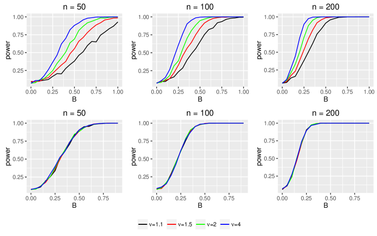
Figure 2: Power function of the test for n=50, 100, 200. First row: under setup 1; second row: under setup 2

Similarly for setup 2, the power of the test goes up when sample size $n$ and $||\beta_{0}||_{\Gamma}$ increase. However the effect of the decay rate $\nu$ can be hardly seen this time. The reason is that when choosing $\zeta$ we did not normalize it as we did in setup1. Therefore even though a larger $\nu$ could lead to a more powerful test, the magnitude of $X(s)$ is significantly decreased due to the faster decay rate, and this counter balanced the effect of $\nu$.

4.2 California air quality data

Back to the California air quality example, as mentioned in the introduction, we are interest in testing the effect of trajectories of oxides of nitrogen ($\text{NO}_{\text{x}}$) on the level of ground-level concentrations of ozone ($\text{O}_{3}$). Data we are using is from the database of California Air Quality Data. $\text{NO}_{\text{x}}$ levels and $\text{O}_{3}$ levels of city Sacramento are recorded from June 1 to August 31 in 2015. There are 91 days on the record, and 3 days are removed due to severe missing data. For the rest 89 days, levels of $\text{NO}_{\text{x}}$ are observed at each hour except for 4am and average $\text{O}_{3}$ level can also be obtained through the recorded data. The left panel of Figure 1 displays the daily trajectories of $\text{NO}_{\text{x}}$ levels, and the middle panel shows the average $\text{O}_{3}$ level each day during the same time period. When applying the proposed testing procedure, every record is rescaled by multiplying 100 due to the small magnitude.

Let $X_{i}(s),\,i=1,...,89$ denote the daily trajectories of $\text{NO}_{\text{x}}$ levels after pre-smoothing and centering, and rescale $s$ so that $s\in[0,1]$. In the introduction, two types of response variables are considered, the average $\text{O}_{3}$ level of the same day as the $\text{NO}_{\text{x}}$ level, and the average $\text{O}_{3}$ level five days later after the recorded $\text{NO}_{\text{x}}$ trajectory. More generally we can examine the relation between the $\text{O}_{3}$ level of a certain day and the $\text{NO}_{\text{x}}$ level $d$ days before that day. If we take $Y_{i},\ i=1,...,89$ as the corresponding $\text{O}_{3}$ level of the day when $X_{i}$ is recorded. Then the regression function is written as

$$Y_{i+d}=\int_{0}^{1}X_{i}(s)\beta(s)ds+\epsilon_{i},$$

for a fixed $d$.

We go through the proposed testing procedure for $d=0,1,...,5$ and all the p-value are listed in Table 2. We can see that for $d$ up to 4, the test returns a significant result at level $\alpha=0.05$, which indicates that daily $\text{NO}_{\text{x}}$ level is significantly related to the $\text{O}_{3}$ level up to four days later. It is also interesting to see that the smallest p-value occurs at $d=1$. A possible way to interpret it is that instead of the current $\text{NO}_{\text{x}}$ level, the average $\text{O}_{3}$ level depends more on the $\text{NO}_{\text{x}}$ level the day before. That is to say there is a delayed effect of $\text{NO}_{\text{x}}$ level on $\text{O}_{3}$ level.

Table 2: P-value

d	0	1	2	3	4	5	6
p-value	3.07e-5	6.78e-9	2.30e-5	3.13e-4	0.0031	0.36	0.70

5 Discussion

We have so far focused on the case with continuously observed functional predictors. If we have densely observed functional predictors, our framework can be applied similarly. An interesting extension of the current work would be to study the case when having sparsely observed functional predictors with/without measurement error. The ideas of Yao et al. (2005a) can be applied. A common strategy is to first have a pre-smoothing step and then apply our methodology. How the number of sparse observations affects the power of the test is beyond the scope of this paper and will be explored in future works.

A continuation of this paper is to study the optimal testing for the generalized functional linear model with a scalar response and a functional predictor (Du and Wang, 2014). Given the functional predictor, the response is assumed to follow some distribution from the exponential family. The main difficulty is that the characterization conditions of the slope estimator becomes complex and nontrivial. This problem hinders further studies in the asymptotic properties. We conjecture that the generalized likelihood ratio test will achieve the optimal rate of testing and the optimal rate still depends on the decay rate of $K^{1/2}\Gamma K^{1/2}$. This issue will be addressed in detail in the future.

6 Proofs of Theorems

6.1 Proof of Theorem 1

We prove this theorem using the calculus of variation. Denote

$$L(\beta)=\frac{1}{n}\sum_{i=1}^{n}\Big{\{}Y_{i}-\int_{0}^{1}X_{i}(s)\beta(s)ds\Big{\}}^{2}+\lambda\int_{0}^{1}\Big{\{}\beta^{(m)}(s)\Big{\}}^{2}ds.$$

For any $\beta,\beta_{1}\in W_{2}^{m}$ and $\delta\in\mathbb{R}$,

$$L(\beta+\delta\beta_{1})-L(\beta)=2\delta L_{1}(\beta,\beta_{1})+O(\delta^{2}),$$ (9)

where

$$L_{1}(\beta,\beta_{1}) = -\frac{1}{n}\sum_{i=1}^{n}\big{\{}Y_{i}-\int_{0}^{1}X_{i}(s)\beta(s)ds\big{\}}\big{\{}\int_{0}^{1}X_{i}(s)\beta_{1}(s)ds\big{\}}$$

$$~{}~{}~{}~{}~{}~{}~{}~{}~{}~{}~{}+\lambda\int_{0}^{1}\beta^{(m)}(s)\beta_{1}^{(m)}(s)ds.$$

By Lemma 1, if $L_{1}(\beta,\beta_{1})=0$ for all $\beta_{1}\in W_{2}^{m}$, letting $\mathcal{I}_{1}=\{t\in[0,1]:L_{2}(\beta)\neq 0\}$ and $\beta_{1}^{(m)}(t)=-I_{\mathcal{I}_{1}}(t)$ gives

$$L_{1}(\beta,\beta_{1})=\int_{\mathcal{I}_{1}}L_{2}(\beta)dt\neq 0,$$

unless $\mathcal{I}_{1}$ is of measure zero. This shows $L_{2}(\beta)=0$ a.e.. This complete the proof of the first part of the theorem.

If $\hat{\beta}$ is the optimal solution, we have

$$\hat{\beta}^{(m)}=\frac{(-1)^{m}}{n}\hat{Q}^{+}\hat{U}^{T}{\bf Y}.$$

It follows from (19) that

$$\hat{H}\widehat{\Upsilon}(1)+\frac{(-1)^{m}}{n}\widetilde{X}(1)\int_{0}^{1}T_{0}^{m}{\bf X}(s)\hat{\beta}^{(m)}(s)ds=\frac{1}{n}\widetilde{X}(1){\bf Y}.$$

Therefore, the second part of the theorem follows from these two facts.

6.2 Proof of Theorem 2

For part (a), under $H_{0}$ with $\beta_{0}\equiv 0$, we have

$$\frac{1}{n}\mbox{RSS}_{0} =\frac{1}{n}\epsilon^{T}\epsilon,$$

$$\frac{1}{n}\mbox{RSS}_{1} =\frac{1}{n}\epsilon^{T}\epsilon+\|\hat{\beta}-\beta_{0}\|_{\hat{\Gamma}}^{2}-\frac{2}{n}\epsilon^{T}\int(\hat{\beta}-\beta_{0}){\bf X}.$$

It follows from Lemma 2 that,

$$\frac{1}{n}\mbox{RSS}_{1} -\frac{1}{n}\mbox{RSS}_{0}$$

$$= \|\hat{\beta}-\beta_{0}\|_{\hat{\Gamma}}^{2}-\frac{2}{n}\epsilon^{T}\int(\hat{\beta}-\beta_{0}){\bf X}$$

$$= \frac{1}{n^{2}}\epsilon^{T}\Big{\{}\int_{0}^{1}\int_{0}^{1}\hat{Q}^{+}\hat{U}(t)\hat{Q}(t,s)\hat{Q}^{+}\hat{U}(s)^{T}dtds-2\int_{0}^{1}\hat{U}(t)\hat{Q}^{+}\hat{U}(t)^{T}dt\Big{\}}\epsilon$$

$$-\frac{1}{n^{2}}\epsilon^{T}\widetilde{X}(1)^{T}\hat{H}^{-1}\widetilde{X}(1)\epsilon$$

$$= -\frac{2}{n}\epsilon^{T}A_{n}\epsilon=o_{p}(n^{-1/2}),$$

provided that $tr(A_{n}^{2})=o(n)$. Hence, with the fact that under $H_{0}$, $\sigma^{2}=\mbox{RSS}_{0}/n+O_{p}(n^{-1/2})$, the likelihood ratio test statistic $\tau_{n,\lambda}$ becomes

$$\tau_{n,\lambda} =-\frac{n}{2}\log\frac{\mbox{RSS}_{1}/n}{\mbox{RSS}_{0}/n}=-\frac{n}{2\sigma^{2}}\Big{(}\frac{1}{n}\mbox{RSS}_{1}-\frac{1}{n}\mbox{RSS}_{0}\Big{)}\big{(}1+o_{p}(n^{-\frac{1}{2}})\big{)}$$

$$=z^{T}A_{n}z+o_{p}(1),$$

where $z=\epsilon/\sigma$.

To show that $\tau_{n,\lambda}$ has an asymptotic normal distribution with mean $\mu_{n}=tr(A_{n})$ and variance $\sigma_{n}^{2}=2tr(A_{n}^{2})$, we need to show that

$$Trace(A_{n}^{4})/\sigma_{n}^{4}\rightarrow 0.$$

Let

$$A_{I}=\frac{1}{n}\int_{0}^{1}\hat{U}(t)\hat{Q}^{+}\hat{U}(t)^{T}dt-\frac{1}{2n}\int_{0}^{1}\int_{0}^{1}\hat{Q}^{+}\hat{U}(t)\hat{Q}(t,s)\hat{Q}^{+}\hat{U}(s)^{T}dtds,$$

and

$$A_{II}=\frac{1}{2}B.$$

So $tr(A)=tr(A_{I})+tr(A_{II})$. Noting that $tr(A_{II})=m/2$, $tr(A)$ is of the same order as $tr(A_{I})$. Recall that $\hat{Q}(t,s)=\sum_{j=1}^{\infty}\hat{\kappa}_{j}\hat{\phi}_{j}(t)\hat{\phi}_{j}(s)$. and $\hat{U}_{X_{i}}(t)=\sum_{k=1}^{\infty}\hat{\xi}_{ik}\hat{\phi}_{k}(t)$ with $n^{-1}\sum_{i=1}^{n}\hat{\xi}_{ik}^{2}=\hat{\kappa}_{k}$ and $n^{-1}\sum_{i=1}^{n}\hat{\xi}_{ik}\hat{\xi}_{ij}=0$ for $k\neq j$. Therefore

$$(A_{I})_{ij}=\frac{1}{n}\sum_{k=1}^{\infty}\frac{(2\lambda+\hat{\kappa}_{k})\hat{\xi}_{ik}\hat{\xi}_{jk}}{2(\lambda+\hat{\kappa}_{k})^{2}}.$$

Further

$$tr(A_{I}) =\sum_{k=1}^{\infty}\frac{\hat{\kappa}_{k}(2\lambda+\hat{\kappa}_{k})}{2(\lambda+\hat{\kappa}_{k})^{2}}\asymp\sum_{k=1}^{\infty}\frac{\hat{\kappa}_{k}}{\lambda+\hat{\kappa}_{k}}.$$

Similarly, we can show that

$$(A_{I}^{2})_{ij}=\frac{1}{n}\sum_{k=1}^{\infty}\frac{(2\lambda+\hat{\kappa}_{k})^{2}\hat{\kappa}_{k}\hat{\xi}_{ik}\hat{\xi}_{jk}}{4(\lambda+\hat{\kappa}_{k})^{4}},\quad\text{ \quad}(A_{I}^{4})_{ij}=\frac{1}{n}\sum_{k=1}^{\infty}\frac{(2\lambda+\hat{\kappa}_{k})^{4}(\hat{\kappa}_{k})^{3}\hat{\xi}_{ik}\hat{\xi}_{jk}}{16(\lambda+\hat{\kappa}_{k})^{8}},$$

and

$$tr(A_{I}^{2})\asymp\sum_{k=1}^{\infty}\frac{\hat{\kappa}_{k}^{2}}{(\lambda+\hat{\kappa}_{k})^{2}},\quad\text{ \quad}tr(A_{I}^{4})\asymp\sum_{k=1}^{\infty}\frac{\hat{\kappa}_{k}^{4}}{(\lambda+\hat{\kappa}_{k})^{4}}.$$

Since $\frac{\hat{\kappa}_{k}^{4}}{(\lambda+\hat{\kappa}_{k})^{4}}\leq\frac{\hat{\kappa}_{k}^{2}}{(\lambda+\hat{\kappa}_{k})^{2}}$, therefore $tr(A_{n}^{4})=O(\sigma_{n}^{2})$, and further $tr(A_{n}^{4})/\sigma_{n}^{4}\rightarrow 0$.

For part (b), Under $H^{\prime}_{1}$,

$$\frac{1}{n}\mbox{RSS}_{0} =\frac{1}{n}\epsilon^{T}\epsilon+\|\beta_{0}\|_{\hat{\Gamma}}^{2}+\frac{2}{n}\epsilon^{T}\int\beta_{0}{\bf X},$$

$$\frac{1}{n}\mbox{RSS}_{1} =\frac{1}{n}\epsilon^{T}\epsilon+\|\hat{\beta}-\beta_{0}\|_{\hat{\Gamma}}^{2}-\frac{2}{n}\epsilon^{T}\int(\hat{\beta}-\beta_{0}){\bf X}$$

$$=\sigma^{2}-\frac{2}{n}\epsilon^{T}A\epsilon$$

$$\qquad+\lambda^{2}\int_{0}^{1}\int_{0}^{1}\hat{Q}(t,s)\hat{Q}^{+}\beta_{0}^{(m)}(t)\hat{Q}^{+}\beta_{0}^{(m)}(s)dtds$$

$$\qquad+(-1)^{m}\frac{2\lambda}{n}\epsilon^{T}\int_{0}^{1}\hat{U}(t)\hat{Q}^{+}\beta_{0}^{(m)}(t)dt-\frac{2}{n}\epsilon^{T}\int\beta_{0}{\bf X}$$

$$\qquad+(-1)^{m+1}\frac{2\lambda}{n}\epsilon^{T}\int_{0}^{1}\int_{0}^{1}\hat{Q}(t,s)\hat{Q}^{+}\beta_{0}^{(m)}(t)\hat{Q}^{+}\hat{U}(s)dtds.$$

For $\frac{1}{n}\mbox{RSS}_{0}$,

$$Var(\frac{2}{n}\epsilon^{T}\int\beta_{0}{\bf X})=\frac{4}{n^{2}}Var(\sum_{i=1}^{n}\epsilon_{i}\int\beta_{0}X_{i})=\frac{4\sigma^{2}}{n^{2}}\sum_{i=1}^{n}\{\int\beta_{0}(s)X_{i}(s)ds\}^{2}=O(\frac{1}{n}||\beta_{0}||_{\hat{\Gamma}}^{2}).$$

For $\frac{1}{n}\mbox{RSS}_{1}$, write $\beta_{0}^{(m)}(t)=\sum_{j=1}^{\infty}\hat{\eta}_{j}\hat{\phi}_{j}(t)$. Since $\beta_{0}^{(m)}\in L_{2}$, we have $\sum_{j=1}^{\infty}\hat{\eta}_{j}^{2}<\infty$. In the above expansion of $\frac{1}{n}\mbox{RSS}_{1}$,

$$\lambda^{2}\int_{0}^{1}\int_{0}^{1}\hat{Q}(t,s) \hat{Q}^{+}\beta_{0}^{(m)}(t)\hat{Q}^{+}\beta_{0}^{(m)}(s)dtds$$

$$= \lambda^{2}\sum_{j=1}^{\infty}\frac{\hat{\kappa}_{j}\hat{\eta}_{j}^{2}}{(\lambda+\hat{\kappa}_{j})^{2}}\leq\lambda^{2}\sum_{j=1}^{\infty}\hat{\eta}_{j}^{2}\sup_{x\geq 0}\frac{x}{(\lambda+x)^{2}}\leq\frac{\lambda}{4}\sum_{j=1}^{\infty}\hat{\eta}_{j}^{2}=O(\lambda).$$

Further,

$$(-1)^{m}\frac{2\lambda}{n}\epsilon^{T}\int_{0}^{1}\hat{U}(t)\hat{Q}^{+}\beta_{0}^{(m)}(t)dt=(-1)^{m}\frac{2\lambda}{n}\sum_{i=1}^{n}\epsilon_{i}\sum_{k=1}^{\infty}\frac{\hat{\xi}_{ik}\hat{\eta}_{k}}{\lambda+\hat{\kappa}_{k}},$$

and its variance is

$$\frac{4\lambda^{2}\sigma^{2}}{n}\sum_{k=1}^{\infty}\frac{\hat{\kappa}_{k}\eta_{k}^{2}}{(\lambda+\hat{\kappa}_{k})^{2}}\leq\frac{4\lambda^{2}\sigma^{2}}{n}\sup_{x\geq 0}\frac{x}{(\lambda+x)^{2}}\sum_{j=1}^{\infty}\hat{\eta}_{j}^{2}\leq\frac{\lambda\sigma^{2}}{n}\sum_{j=1}^{\infty}\hat{\eta}_{j}^{2}=O(\lambda/n).$$

The last term becomes

$$(-1)^{m+1}\frac{2\lambda}{n}\epsilon^{T}\int_{0}^{1}\int_{0}^{1}\hat{Q}(t,s)\hat{Q}^{+}\beta_{0}^{(m)}(t)\hat{Q}^{+}\hat{U}(s)dtds=(-1)^{m+1}\frac{2\lambda}{n}\sum_{i=1}^{n}\epsilon_{i}\sum_{k=1}^{\infty}\frac{\hat{\kappa}_{k}\hat{\eta}_{k}\hat{\xi}_{ik}}{(\lambda+\hat{\kappa}_{k})^{2}}.$$

Since $\sum_{k=1}^{\infty}\frac{\hat{\kappa}_{k}\hat{\eta}_{k}\hat{\xi}_{ik}}{(\lambda+\hat{\kappa}_{k})^{2}}\leq\sum_{k=1}^{\infty}\frac{\hat{\eta}_{k}\hat{\xi}_{ik}}{\lambda+\hat{\kappa}_{k}}$, the variance of last term is controlled by $O(\lambda/n)$. So altogether,

$$\frac{1}{n}\mbox{RSS}_{1}-\frac{1}{n}\mbox{RSS}_{0}=-\frac{2}{n}\epsilon^{T}A\epsilon-\|\beta_{0}\|_{\hat{\Gamma}}^{2}+O\Big{(}\lambda\Big{)}+O_{p}\Big{(}n^{-1/2}\lambda^{1/2}\Big{)}+O_{p}\Big{(}n^{-1/2}\|\beta_{0}\|_{\hat{\Gamma}}\Big{)}.$$

Since $\rho_{n}^{2}=o(n^{-1/2})$ and $\lambda=o(n^{-1/2})$, therefor $\frac{1}{n}\mbox{RSS}_{1}-\frac{1}{n}\mbox{RSS}_{0}=o_{p}(n^{-1/2})$ and

$$\tau_{n,\lambda}=z^{T}Az+\frac{n}{2\sigma^{2}}\|\beta_{0}\|_{\hat{\Gamma}}^{2}+O\Big{(}n\lambda\Big{)}+O_{p}\Big{(}n^{1/2}\lambda^{1/2}\Big{)}+O_{p}\Big{(}n^{1/2}\|\beta_{0}\|_{\hat{\Gamma}}\Big{)}.$$

6.3 Proof of Theorem 3

The proof follows Ingster (1993). First show part (a). Let

$$\rho_{n}=n^{-2r/(1+4r)},$$

and suppose that $\rho_{n}^{\prime}/\rho_{n}\rightarrow 0$. We show that, for any test $\phi_{n}$,

$$\lim\inf_{n\rightarrow\infty}\gamma_{n}(\phi_{n},\rho_{n}^{\prime})\geq 1.$$

The idea of deriving the lower bound is standard. Let $\pi_{n}$ be a probability measure on ${\cal F}_{K,\Gamma}(\rho_{n}^{\prime})$. Then the lower bound is based on the inequality

$$\sup_{f\in{\cal F}_{K,\Gamma}(\rho_{n}^{\prime})}\mathbb{P}_{f}(\phi_{n}=0)\geq\mathbb{P}_{f,\pi_{n}}(\phi_{n}=0),$$

where $\mathbb{P}_{f,\pi_{n}}=\int\mathbb{P}_{f}d\pi_{n}$. Write

$$\gamma_{n,\pi_{n}}=\mathbb{P}_{0}(\phi_{n}=1)+\mathbb{P}_{f,\pi_{n}}(\phi_{n}=0).$$

Denote by $\ell_{n,\pi_{n}}$ the likelihood ratio,

$$\ell_{n,\pi_{n}}=\frac{d~{}\mathbb{P}_{f,\pi_{n}}}{d~{}\mathbb{P}_{0}}=\int\frac{d~{}\mathbb{P}_{f}}{d~{}\mathbb{P}_{0}}d\pi_{n}.$$

For any $f\in{\cal F}_{K,\Gamma}(\rho_{n})$, direct calculation yields that

$$\log\frac{d~{}\mathbb{P}_{f}}{d~{}\mathbb{P}_{0}}=\frac{1}{\sigma^{2}}\sum_{i=1}^{n}Y_{i}\int X_{i}f-\frac{n}{2\sigma^{2}}\|f\|_{\hat{\Gamma}}^{2},$$

where $\hat{\Gamma}$ is the empirical covariance function such as

$$\hat{\Gamma}(t,s)=\frac{1}{n}\sum_{i=1}^{n}X_{i}(t)X_{i}(s).$$

It is convenient to use the following inequalities Ingster (1987):

$$\gamma_{n,\pi_{n}}(\phi_{n},\rho_{n}^{\prime})=1-\frac{1}{2}\mbox{var}(\mathbb{P}_{0},\mathbb{P}_{f,\pi_{n}})\geq 1-\frac{1}{2}\delta_{n,\pi_{n}},$$

where $\mbox{var}(\mathbb{P}_{0},\mathbb{P}_{f,\pi_{n}})$ stands for $L_{1}$ distance between two measures, and

$$\delta_{n,\pi_{n}}^{2}=\mathbb{E}_{0}(\ell_{n,\pi_{n}}-1)^{2}.$$

In the following, we select a probability measure $\pi_{n}$ for which $\gamma_{n,\pi_{n}}$ can be effectively estimated. Recall that $K=TT^{*}$, where $T^{*}$ is the adjoint operator to $T$ such that $\langle f,Tg\rangle=\langle T^{*}f,g\rangle$. Define the linear operator $T\hat{\Gamma}T^{*}$ and let $\hat{s}_{1}\geq\hat{s}_{2}\geq\cdots\geq 0$ be the eigenvalues of $T\hat{\Gamma}T^{*}$ and the $\hat{\varphi}_{k}$ be the corresponding eigenfunctions. Consider

$$f_{\xi}=u\sum_{k=1}^{M}\xi_{k}g_{k},$$ (11)

where $\xi=(\xi_{1},\ldots,\xi_{M})$ and $\xi_{k}=\pm 1$ with probability $1/2$, and $g_{k}=\hat{s}_{k}^{-1/2}T^{*}\hat{\varphi}_{k}$. In (11), we choose $M=2n^{2/(4r+1)}$ and $u=n^{-1/(4r+1)}\rho_{n}^{\prime}$. Note that

$$\Big{\langle}g_{k},g_{j}\Big{\rangle}_{\hat{\Gamma}}=(\hat{s}_{k}\hat{s}_{j})^{-1/2}\Big{\langle}T^{*}\hat{\varphi}_{k},T^{*}\hat{\varphi}_{j}\Big{\rangle}_{\hat{\Gamma}}=(\hat{s}_{k}\hat{s}_{j})^{-1/2}\Big{\langle}T{\hat{\Gamma}}T^{*}\hat{\varphi}_{k},\hat{\varphi}_{j}\Big{\rangle}_{L_{2}}=\delta_{jk},$$

where $\delta_{jk}=1$ for $j=k$, and $0$ for $j\neq k$. Further,

$$\Big{\langle}g_{k},g_{j}\Big{\rangle}_{{\cal H}(K)}=(\hat{s}_{k}\hat{s}_{j})^{-1/2}\Big{\langle}T^{*}\hat{\varphi}_{k},T^{*}\hat{\varphi}_{j}\Big{\rangle}_{{\cal H}(K)}=(\hat{s}_{k}\hat{s}_{j})^{-1/2}\Big{\langle}\hat{\varphi}_{k},\hat{\varphi}_{j}\Big{\rangle}_{L_{2}}=(\hat{s}_{k}\hat{s}_{j})^{-1/2}\delta_{jk}.$$

It is easy to check that

$$\|f_{\xi}\|_{{\cal H}(K)}^{2}=u^{2}\sum_{k=1}^{M}\hat{s}_{k}^{-1}\leq u^{2}M\hat{s}_{M}^{-1}=2(\rho_{n}^{\prime})^{2}s_{M}^{-1}(1+o_{p}(1)),$$

which is bounded since $s_{M}$ has the same order with $\rho_{n}^{2}=n^{-4r/(4r+1)}$ and $\rho_{n}^{\prime}/\rho_{n}=o(1)$. For any $\varphi\in L_{2}$, $T^{*}\varphi\in{\cal H}(K)$ (Cucker and Smale, 2002). Therefore, $f_{\xi}\in{\cal H}(K)$. On the other hand,

$$\|f_{\xi}\|_{\hat{\Gamma}}^{2}=Mu^{2}=2(\rho_{n}^{\prime})^{2}.$$

So, $\|f_{\xi}\|_{\Gamma}^{2}=2(\rho_{n}^{\prime})^{2}(1+o(1))\geq(\rho_{n}^{\prime})^{2}$ and it shows that $f_{\xi}\in{\cal F}_{K,\Gamma}(\rho_{n}^{\prime})$.

For this case, the likelihood ratio is

$$\ell_{n,\pi_{n}} =\mathbb{E}_{\xi}\frac{d~{}\mathbb{P}_{f_{\xi}}}{d~{}\mathbb{P}_{0}}=\exp\Big{(}-\frac{nMu^{2}}{2\sigma^{2}}\Big{)}\mathbb{E}_{\xi}\exp(\frac{u}{\sigma^{2}}\sum_{k=1}^{M}\sum_{i=1}^{n}Y_{i}x_{ik}\xi_{k})$$

$$=\exp\Big{(}-\frac{nMu^{2}}{2\sigma^{2}}\Big{)}\prod_{k=1}^{M}cosh(\frac{u}{\sigma^{2}}\sum_{k=1}^{M}Y_{i}x_{ik}).$$

where $x_{ik}$ is denoted as $x_{ik}=\int X_{i}g_{k}$. Note that $\sum_{i=1}^{n}x_{ik}^{2}=n\|g_{k}\|_{\hat{\Gamma}}^{2}=n$. Given $X_{1},\ldots,X_{n}$, we have

$$\mathbb{E}_{0}\Big{(}\ell_{n,\pi_{n}}\Big{|}X_{1},\ldots,X_{n}\Big{)} =\mathbb{E}_{0}\mathbb{E}_{\xi}\frac{d~{}\mathbb{P}_{f_{\xi}}}{d~{}\mathbb{P}_{0}}=\mathbb{E}_{\xi}\mathbb{E}_{0}\frac{d~{}\mathbb{P}_{f_{\xi}}}{d~{}\mathbb{P}_{0}}$$

$$=\exp\Big{(}-\frac{nMu^{2}}{2\sigma^{2}}\Big{)}\mathbb{E}_{\xi}\prod_{i=1}^{n}\mathbb{E}_{0}\exp(\frac{u}{\sigma^{2}}\sum_{k=1}^{M}\xi_{k}x_{ik}\cdot Y_{i})$$

$$=\exp\Big{(}-\frac{nMu^{2}}{2\sigma^{2}}\Big{)}\mathbb{E}_{\xi}\prod_{i=1}^{n}\exp\{\frac{1}{2}\sigma^{2}(\frac{u}{\sigma^{2}}\sum_{k=1}^{M}\xi_{k}x_{ik})^{2}\}$$

$$=\exp(-\frac{nMu^{2}}{2\sigma^{2}})\exp(\frac{nMu^{2}}{2\sigma^{2}})=1.$$

Noting that

$$\ell_{n,\pi_{n}}^{2} =\exp\Big{(}-\frac{nMu^{2}}{\sigma^{2}}\Big{)}\prod_{k=1}^{M}cosh(\frac{u}{\sigma^{2}}\sum_{k=1}^{M}Y_{i}x_{ik})^{2}$$

$$=\exp\Big{(}-\frac{nMu^{2}}{\sigma^{2}}\Big{)}\prod_{k=1}^{M}(\frac{1}{4}e^{\frac{2u}{\sigma^{2}}\sum_{k=1}^{M}Y_{i}x_{ik}}+\frac{1}{4}e^{-\frac{2u}{\sigma^{2}}\sum_{k=1}^{M}Y_{i}x_{ik}}+\frac{1}{2})$$

$$=\exp\Big{(}-\frac{nMu^{2}}{\sigma^{2}}\Big{)}\mathbb{E}_{\varsigma}\exp(\frac{2u}{\sigma^{2}}\sum_{k=1}^{M}\sum_{i=1}^{n}Y_{i}x_{ik}\varsigma_{k}),$$

where random variable $\varsigma$ takes value $-1,0,1$ with probability $1/4,\,1/2,\,1/4$. Therefore we can calculate $\mathbb{E}_{0}\Big{(}\ell_{n,\pi_{n}}^{2}\Big{|}X_{1},\ldots,X_{n}\Big{)}$ as

$$\mathbb{E}_{0}\Big{(}\ell_{n,\pi_{n}}^{2}\Big{|}X_{1},\ldots,X_{n}\Big{)} =\mathbb{E}_{0}\exp\Big{(}-\frac{nMu^{2}}{\sigma^{2}}\Big{)}\mathbb{E}_{\varsigma}\exp(\frac{2u}{\sigma^{2}}\sum_{k=1}^{M}\sum_{i=1}^{n}Y_{i}x_{ik}\varsigma_{k})$$

$$=\exp\Big{(}-\frac{nMu^{2}}{\sigma^{2}}\Big{)}\mathbb{E}_{\varsigma}\prod_{i=1}^{n}\mathbb{E}_{0}\exp(\frac{2u}{\sigma^{2}}\sum_{k=1}^{M}x_{ik}\varsigma_{k}\cdot Y_{i})$$

$$=\exp\Big{(}-\frac{nMu^{2}}{\sigma^{2}}\Big{)}\mathbb{E}_{\varsigma}\exp(\frac{2u^{2}n}{\sigma^{2}}\sum_{k=1}^{M}\varsigma_{k}^{2})$$

$$=\exp\Big{(}-\frac{nMu^{2}}{\sigma^{2}}\Big{)}\prod_{k=1}^{M}\{\frac{1}{2}\exp(\frac{2u^{2}n}{\sigma^{2}})+\frac{1}{2}\}$$

$$=\{\cosh(\frac{u^{2}n}{\sigma^{2}})\}^{M},$$

and

$$\mathbb{E}_{0}(\ell_{n,\pi_{n}}-1)^{2} =\mathbb{E}_{0}\Big{(}\ell_{n,\pi_{n}}^{2}\Big{|}X_{1},\ldots,X_{n}\Big{)}-2\mathbb{E}_{0}\Big{(}\ell_{n,\pi_{n}}\Big{|}X_{1},\ldots,X_{n}\Big{)}+1$$

$$=\{\cosh(\frac{u^{2}n}{\sigma^{2}})\}^{M}-1.$$

Using the inequality $\log\cosh x\leq Bx^{2}$ for a certain $B$,

$$\{\cosh(\frac{u^{2}n}{\sigma^{2}})\}^{M}-1 \leq\exp\Big{(}\frac{BMu^{4}n^{2}}{\sigma^{4}}\Big{)}-1.$$

Hence

$$\mathbb{E}_{0}(\ell_{n,\pi_{n}}-1)^{2}\leq\exp\Big{(}\frac{Bn^{2}Mu^{4}}{\sigma^{4}}\Big{)}-1.$$

Our choices of $M$ and $u$ guarantees that $n^{2}Mu^{4}\rightarrow 0$, so $\lim\inf_{n\rightarrow}\gamma_{n}(\phi_{n},\rho_{n}^{\prime})=1$. This completes the proof of part (a).

Next, we prove part (b). The proof is similar. In particular, in (11) we choose $M=\log n/(2r)$ and $u=2\rho_{n}^{\prime}\sqrt{2r/\log n}$, where $\rho_{n}^{\prime}/\rho_{n}\rightarrow 0$ with $\rho_{n}=n^{-1/2}(\log n/(2r))^{1/4}$. It is easy to see that $n^{2}Mu^{4}\rightarrow 0$, so that $\lim\inf_{n\rightarrow}\gamma_{n}(\phi_{n},\rho_{n}^{\prime})=1$. This completes the proof of part (b).

6.4 Proof of Theorem 4

Recall that $H^{\prime}_{1}:{\cal F}^{\prime}_{K,\Gamma}(\rho_{n})=\big{\{}\beta\in\mathcal{H}(K):~{}\|\beta\|_{\Gamma}=\rho_{n}\big{\}}$, we only need to show that

$$\lim_{c_{n}\rightarrow\infty}\inf_{\beta_{0}\in{\cal F}^{\prime}_{K,\Gamma}(c_{n}\rho_{n})}\mathbb{P}_{\beta_{0}}\Big{(}\frac{\tau_{n,\lambda}-\mu_{n}}{\sigma_{n}}>z_{\alpha}\Big{)}=1.$$

The power function under $H_{1}^{\prime}$ can be written as

$$\mathbb{P}_{\beta_{0}}\Big{(}\frac{\tau_{n,\lambda}-\mu_{n}}{\sigma_{n}}\geq z_{\alpha}\Big{)}$$

$$= \mathbb{P}_{\beta_{0}}\Big{\{}\frac{z^{T}Az-\mu_{n}}{\sigma_{n}}+\frac{\frac{n}{2\sigma^{2}}\|\beta_{0}\|_{\hat{\Gamma}}^{2}+O\Big{(}n\lambda\Big{)}+O_{p}\Big{(}n^{1/2}\lambda^{1/2}\Big{)}+O_{p}\Big{(}n^{1/2}\|\beta_{0}\|_{\hat{\Gamma}}\Big{)}}{\sigma_{n}}\geq z_{\alpha}\Big{\}}.$$

Recall that $\sigma_{n}^{2}=tr(A^{2})=O(tr(A))$ as shown in the proof as Theorem 2, and by Lemma 3, we have

$$\mu_{n}=O_{p}(\sum_{k=1}^{\infty}\frac{s_{k}}{\lambda+s_{k}})\quad\quad and\quad\quad\sigma_{n}^{2}=O_{p}(\sum_{k=1}^{\infty}\frac{s_{k}}{\lambda+s_{k}}).$$

Therefore $\mu_{n}$ and $\sigma_{n}^{2}$ are of order $O_{p}(\lambda^{-1/2r}$) when $s_{k}\asymp k^{-2r}$, or of order $O_{p}\{(2r)^{-1}\log\lambda^{-1}\}$ when $s_{k}\asymp e^{-2rk}$. Recall that when $\kappa_{k}\asymp k^{-2r}$, the optimal $\lambda$ is of order $n^{-4r/(4r+1)}$; when $\kappa_{k}\asymp exp^{-2rk}$, $\log\lambda^{-1}=O(\log n)$. So, when $\kappa_{k}\asymp k^{-2r}$,

$$\lim_{c_{n}\rightarrow\infty}\inf_{\beta\in{\cal F}_{K,\Gamma}:\|\beta\|_{\Gamma}\geq c_{n}n^{-2r/(4r+1)}}\mathbb{P}_{\beta}\Big{(}\frac{\tau_{n,\lambda}-\mu_{n}}{\sigma_{n}}\geq z_{\alpha}\Big{)}=1,$$

and when $\kappa_{k}\asymp e^{-2rk}$,

$$\lim_{c_{n}\rightarrow\infty}\inf_{\beta\in{\cal F}_{K,\Gamma}:\|\beta\|_{\Gamma}\geq c_{n}\{\log n/(2rn^{2})\}^{1/4}}\mathbb{P}_{\beta}\Big{(}\frac{\tau_{n,\lambda}-\mu_{n}}{\sigma_{n}}\geq z_{\alpha}\Big{)}=1.$$

This finishes the proof of the theorem.

6.5 Proof of Theorem 5

First noting that $s_{k}$ and $\kappa_{k}$ have the same decay rate, so we can replace $s_{k}$ in condition $s_{k}\asymp k^{-2r}$ by $\kappa_{k}$.

Given a symmetric bivariate function $M$, let $|||M|||=(\int\int M^{2})^{1/2}$. Define $\delta_{k}=\min_{1\leq j\leq k}(\kappa_{j}-\kappa_{j+1})$ which is of order $k^{-2r-1}$. $\tilde{\Delta}=|||\tilde{Q}-Q|||$, $\tilde{\Delta}_{j}=\|\int(\tilde{Q}-Q)\phi_{j}\|$, and

$$\tilde{\Delta}_{jj}=\int_{0}^{1}\int_{0}^{1}(\tilde{Q}(t,s)-Q(t,s))\phi_{j}(t)\phi_{j}(s)dtds.$$

It follows from Equation (5.7) of Hall and Horowitz (2007) that

$$\Big{|}\tilde{\kappa}_{j}-\kappa_{j}-\tilde{\Delta}_{jj}\Big{|}\leq\delta_{j}^{-1}\tilde{\Delta}(\tilde{\Delta}+\tilde{\Delta}_{j}),$$

and we also have $\mathbb{E}\tilde{\Delta}_{jj}^{2}\leq C_{1}n^{-1}\kappa_{j}^{2}$ and $\mathbb{E}(\tilde{\Delta}^{2}+\tilde{\Delta}_{j}^{2})\leq C_{2}n^{-1}$ where $C_{1}$ and $C_{2}$ do not depend on $j$. Observe that

$$\sum_{j=1}^{\varrho}|\tilde{\kappa}_{j}-\kappa_{j}|\leq\sum_{j=1}^{\varrho}|\tilde{\Delta}_{j}|+\tilde{\Delta}\sum_{j=1}^{\varrho}\delta_{j}^{-1}(\tilde{\Delta}+\tilde{\Delta}_{j}).$$

Further, $\sum_{j=1}^{\varrho}|\tilde{\Delta}_{jj}|$ is of order $O_{p}(n^{-1/2})$ since

$$\mathbb{E}\sum_{j=1}^{\varrho}|\tilde{\Delta}_{jj}|\leq\sum_{j=1}^{\varrho}\sqrt{\mathbb{E}\tilde{\Delta}_{jj}^{2}}\leq C_{1}n^{-1/2}\sum_{j=1}^{\varrho}\kappa_{j}=O(n^{-1/2}),$$

and $\tilde{\Delta}\sum_{j=1}^{\varrho}\delta_{j}^{-1}(\tilde{\Delta}+\tilde{\Delta}_{j})$ is or order $O_{p}(n^{-1}\varrho^{2r+2})$ since

$$\mathbb{E}\sum_{j=1}^{\varrho}|\delta_{j}^{-1}(\tilde{\Delta}+\tilde{\Delta}_{j})|\leq\sum_{j=1}^{\varrho}\delta_{j}^{-1}\sqrt{2\mathbb{E}(\tilde{\Delta}^{2}+\tilde{\Delta}_{j}^{2})}\leq\sqrt{2C_{2}n^{-1}}\sum_{j=1}^{\varrho}\delta_{j}^{-1}=O(n^{-1/2}\varrho^{2r+2}).$$

Hence,

$$\sum_{j=1}^{\varrho}\Big{|}\tilde{\kappa}_{j}-\kappa_{j}\Big{|}=O_{p}\Big{(}n^{-1/2}+n^{-1}\varrho^{2r+2}\Big{)}.$$

On the other hand, since $E(\tilde{Q}-Q)^{2}=O(n^{-1})$ uniformly on $[0,1]^{2}$,

$$\Big{|}\sum_{j=\varrho+1}^{\infty}(\tilde{\kappa}_{j}-\kappa_{j})\Big{|} =\Big{|}\int\int(\tilde{Q}-Q)(s,t)dsdt-\sum_{j=1}^{\varrho}(\tilde{\kappa}_{j}-\kappa_{j})\Big{|}$$

$$\leq[\int\int(\tilde{Q}-Q)^{2}]^{1/2}+\Big{|}\sum_{j=1}^{\varrho}\Big{(}\tilde{\kappa}_{j}-\kappa_{j}\Big{)}\Big{|}$$

$$=O_{p}(n^{-1/2}+n^{-1}\varrho^{2r+2}).$$

If we choose $\rho\asymp n^{1/(4r+1)}$, we have

$$\Big{|}\sum_{j=1}^{\varrho}(\tilde{\kappa}_{j}-\kappa_{j})\Big{|}=O_{p}(n^{(-2r+1)/(4r+1)}),~{}~{}~{}~{}\Big{|}\sum_{j=\varrho+1}^{\infty}(\tilde{\kappa}_{j}-\kappa_{j})\Big{|}=O_{p}(n^{(-2r+1)/(4r+1)}).$$

Define the event ${\cal E}_{\varrho}$ by

$${\cal E}_{\varrho}={\cal E}_{\varrho}(n)=\{\frac{1}{2}\kappa_{\varrho}\geq\tilde{\Delta}\}.$$

Since $\sup_{k\geq 1}|\tilde{\kappa}_{k}-\kappa_{k}|\leq\tilde{\Delta}$ Bhatia et al. (1983), if ${\cal E}_{\varrho}$ holds, we have $\tilde{\kappa}_{k}\geq\frac{1}{2}\kappa_{k}$ for $1\leq k\leq\varrho$. Here, we choose $\varrho\asymp n^{1/(4r+1)}$, which implies that $n^{1/2}\kappa_{\varrho}\rightarrow\infty$ as $n\rightarrow\infty$. Since $\tilde{\Delta}=O_{p}(n^{-1/2})$, we have $\mathbb{P}({\cal E}_{\varrho})\rightarrow 1$. Therefore, since the result we wish to prove only relates to probabilities of differences (not to moments of differences), it suffices to work with bounds that are established under the assumption that ${\cal E}_{\varrho}$ holds. The optimal choice $\tilde{\lambda}$ is the root of

$$\frac{1}{n}\sum_{k=1}^{\infty}\frac{\tilde{\kappa}_{k}}{(\sqrt{\lambda}+\tilde{\kappa}_{k})^{2}}=2\sqrt{\lambda}.$$

In the following, we derive the asymptotic order of $\sum_{k=1}^{\infty}\frac{\tilde{\kappa}_{k}}{(\sqrt{\lambda}+\tilde{\kappa}_{k})^{2}}$. Note that

$$\sum_{k=1}^{\infty}\frac{\tilde{\kappa}_{k}}{(\sqrt{\lambda}+\tilde{\kappa}_{k})^{2}} =\sum_{k=1}^{\varrho}\frac{\tilde{\kappa}_{k}}{(\sqrt{\lambda}+\tilde{\kappa}_{k})^{2}}+\sum_{k=\varrho+1}^{\infty}\frac{\tilde{\kappa}_{k}}{(\sqrt{\lambda}+\tilde{\kappa}_{k})^{2}}$$

$$\leq\sum_{k=1}^{\varrho}\tilde{\kappa}_{k}^{-1}+\lambda^{-1}\sum_{k=\varrho+1}^{\infty}\tilde{\kappa}_{k}$$

$$\leq 2\sum_{k=1}^{\varrho}\kappa_{k}+\lambda^{-1}\sum_{k=\varrho+1}^{\infty}\kappa_{k}+\lambda^{-1}\Big{|}\sum_{j=\varrho+1}^{\infty}(\tilde{\kappa}_{j}-\kappa_{j})\Big{|}$$

$$=O_{p}\Big{(}n^{(2r+1)/(4r+1)}+\lambda^{-1}n^{(-2r+1)/(4r+1)}\Big{)}.$$ (12)

We also need the lower bound for $\sum_{k=1}^{\infty}\frac{\tilde{\kappa}_{k}}{(\sqrt{\lambda}+\tilde{\kappa}_{k})^{2}}$. This follows from

$$\sum_{k=1}^{\infty}\frac{\tilde{\kappa}_{k}}{(\sqrt{\lambda}+\tilde{\kappa}_{k})^{2}} \geq\sum_{k=\varrho+1}^{\infty}\frac{\tilde{\kappa}_{k}}{(\sqrt{\lambda}+\tilde{\kappa}_{k})^{2}}$$

$$\geq\frac{1}{(\sqrt{\lambda}+\tilde{\kappa}_{\varrho})^{2}}\sum_{k=\varrho+1}^{\infty}\tilde{\kappa}_{k}$$

$$\geq\frac{1}{2(\lambda+O_{p}(n^{-4r/(4r+1)}))}O_{p}(n^{(-2r+1)/(4r+1)}).$$ (13)

Combining (12) and (13), we obtain that $\tilde{\lambda}$ is of order $O_{p}(n^{4r/(4r+1)})$.

7 Proof of Propositions and Lemmas

Proof of Proposition 1. Let ${\cal D}_{k}=\mbox{span}\{f_{1},\ldots,f_{k}:K^{1/2}f_{j}=T^{*}\varphi_{j},j=1,\ldots,k\}$. It follows from the minimax principal that

$$\tilde{s}_{k} \leq\sup_{f\in{\cal D}_{k}^{\perp}}\frac{\Big{\langle}K^{1/2}\Gamma K^{1/2}f,~{}f\Big{\rangle}}{\langle f,f\rangle}=\sup_{f\in{\cal D}_{k}^{\perp}}\frac{\Big{\langle}\Gamma K^{1/2}f,~{}K^{1/2}f\Big{\rangle}}{\langle f,f\rangle}$$

$$=\sup_{g\in\tilde{{\cal D}}_{k}^{\perp}}\frac{\Big{\langle}\Gamma T^{*}g,~{}T^{*}g\Big{\rangle}}{\langle g,g\rangle}\frac{\langle g,g\rangle}{\langle T^{*}g,T^{*}g\rangle}\leq cs_{k},$$

where $\tilde{s}_{k}$ is the $k$th eigenvalue of $K^{1/2}\Gamma K^{1/2}$, $\tilde{{\cal D}}_{k}=\mbox{span}\{\varphi_{1},\ldots,\varphi_{k}\}$ and the constant $c>0$ does not depend on $k$. Using a similar argument, we may show that $s_{k}\leq c\tilde{s}_{k}$. Therefore, the eigenvalues of $T\Gamma T^{*}$ and $K^{1/2}\Gamma K^{1/2}$ have the same decay rate. ∎

Lemma 1.

The following statements are true:

(a). The $\beta\in W_{2}^{m}$ minimizes $L(\beta)$, if and only if, $L_{1}(\beta,\beta_{1})=0$ for all $\beta_{1}\in W_{2}^{m}$.

(b). If $\beta\in W_{2}^{m}$ minimizes $L(\beta)$, then for all $\beta_{1}\in W_{2}^{m}$,

$$L_{1}(\beta,\beta_{1})=\int_{0}^{1}L_{2}(\beta)(t)~{}\beta_{1}^{(m)}(t)dt,$$ (14)

where

$$L_{2}(\beta)=(\lambda I+\hat{Q})\beta^{(m)}-\frac{(-1)^{m}}{n}\hat{U}^{T}{\bf Y}.$$ (15)

Proof.

First show part (a). If $\hat{\beta}\in W_{2}^{m}$ minimizes $L(\beta)$, then $L(\hat{\beta}+\delta\beta_{1})-L(\hat{\beta})\geq 0$ for all $\beta_{1}\in W_{2}^{m}$ and any $\delta\in\mathbb{R}$. Then $L_{1}(\hat{\beta},\beta_{1})=0$ follows since $\delta$ can be either negative or positive. On the other hand, if $L_{1}(\hat{\beta},\beta_{1})=0$, we have $L(\hat{\beta}+\delta\beta_{1})-L(\hat{\beta})\geq 0$ by (9). Thus, $\hat{\beta}$ minimizes $L(\beta)$. Therefore, part (a) follows.

Let $\beta_{1}(t)=t^{(k-1)}$, $k=1,\ldots,m$ in (6.1). If $\hat{\beta}$ minimizes $L(\beta)$, then

$$\frac{1}{n}\sum_{i=1}^{n}\big{\{}Y_{i}-\int_{0}^{1}X_{i}(s)\hat{\beta}(s)ds\big{\}}\big{\{}\int_{0}^{1}X_{i}(s)s^{(k-1)}ds\big{\}}=0.$$ (16)

Let $X_{i}^{(-k)}(t)=T_{0}^{k}X_{i}(t)=\int_{0}^{1}\frac{(t-s)_{+}^{(k-1)}}{(k-1)!}X_{i}(s)ds$. When $k=1$, $\int_{0}^{1}X_{i}(s)s^{(k-1)}ds=X_{i}^{(-1)}(1)$ and further (16) becomes

$$\frac{1}{n}\sum_{i=1}^{n}X_{i}^{(-1)}(1)\big{\{}Y_{i}-\int_{0}^{1}X_{i}(s)\hat{\beta}(s)ds\big{\}}=0.$$

When $k=2$, we have

$$\frac{1}{n}\sum_{i=1}^{n} \big{\{}Y_{i}-\int_{0}^{1}X_{i}(s)\hat{\beta}(s)ds\big{\}}\big{\{}\int_{0}^{1}X_{i}(s)sds\big{\}}$$

$$=-\frac{1}{n}\sum_{i=1}^{n}\big{\{}Y_{i}-\int_{0}^{1}X_{i}(s)\hat{\beta}(s)ds\big{\}}\big{\{}\int_{0}^{1}X_{i}(s)(1-s)ds\big{\}}$$

$$=-\frac{1}{n}\sum_{i=1}^{n}\big{\{}Y_{i}-\int_{0}^{1}X_{i}(s)\hat{\beta}(s)ds\big{\}}\big{\{}X_{i}^{(-2)}(1)\big{\}}.$$

Hence,

$$\frac{1}{n}\sum_{i=1}^{n}X_{i}^{(-2)}(1)\big{\{}Y_{i}-\int_{0}^{1}X_{i}(s)\hat{\beta}(s)ds\big{\}}=0.$$

Following the same procedure, it can be shown that

$$\frac{1}{n}\sum_{i=1}^{n}X_{i}^{(-k)}(1)\big{\{}Y_{i}-\int_{0}^{1}X_{i}(s)\hat{\beta}(s)ds\big{\}}=0,~{}k=1,\ldots,m.$$ (17)

Considering that

$$\beta_{1}(s)=\sum_{k=0}^{m-1}(-1)^{k}\frac{\beta_{1}^{(k)}(1)}{k!}(1-s)^{k}+(-1)^{m}\int_{0}^{1}\frac{\beta_{1}^{(m)}(t)}{(m-1)!}(t-s)_{+}^{m-1}dt.$$

Therefore

$$\int_{0}^{1} X_{i}(s)\beta_{1}(s)ds$$

$$=\sum_{k=0}^{m-1}(-1)^{k}\beta_{1}^{(k)}(1)\int_{0}^{1}X_{i}(s)\frac{(1-s)^{k}}{k!}ds$$

$$\quad\quad+(-1)^{m}\int_{0}^{1}\int_{0}^{1}X_{i}(s)\frac{\beta_{1}^{(m)}(t)}{(m-1)!}(t-s)_{+}^{m-1}dtds$$

$$=\sum_{k=1}^{m}(-1)^{k-1}\beta_{1}^{(k-1)}(1)~{}X_{i}^{(-k)}(1)+(-1)^{m}\int_{0}^{1}\beta_{1}^{(m)}(t)X_{i}^{(-m)}(t)dt.$$ (18)

If (17) holds, direct calculation yields

$$\frac{1}{n}\sum_{i=1}^{n} \big{\{}Y_{i}-\int_{0}^{1}X_{i}(s)\hat{\beta}(s)ds\big{\}}\big{\{}\int_{0}^{1}X_{i}(s)\beta_{1}(s)ds\big{\}}$$

$$=\frac{(-1)^{m}}{n}\sum_{i=1}^{n}\big{\{}Y_{i}-\int_{0}^{1}X_{i}(s)\hat{\beta}(s)ds\big{\}}\big{\{}\int_{0}^{1}X_{i}^{(-m)}(t)\beta_{1}^{(m)}(t)dt\big{\}}.$$

Recall the definition of $L_{2}(\beta)$, we have

$$L_{2}(\hat{\beta}) =\lambda~{}\hat{\beta}^{(m)}(t)+\frac{(-1)^{m}}{n}\sum_{i=1}^{n}X_{i}^{(-m)}(t)\big{\{}\int_{0}^{1}X_{i}(s)\hat{\beta}(s)ds-Y_{i}\big{\}}$$

$$=\lambda~{}\hat{\beta}^{(m)}(t)+\frac{(-1)^{m}}{n}T_{0}^{(m)}{\bf X}(t)^{T}\Big{\{}\int_{0}^{1}{\bf X}(s)\hat{\beta}(s)ds-{\bf Y}\Big{\}}.$$

Similar to (18),

$$\int_{0}^{1}X_{i}(s)\hat{\beta}(s)ds=\widehat{\Upsilon}(1)^{T}\widetilde{X}_{i}(1)+(-1)^{m}\int_{0}^{1}X_{i}^{(-m)}(s)\hat{\beta}^{(m)}(s)ds,~{}~{}~{}j=1,\ldots,m.$$

which gives

$$\int_{0}^{1}{\bf X}(s)\hat{\beta}(s)ds=\widetilde{X}(1)^{T}\widehat{\Upsilon}(1)+(-1)^{m}\int_{0}^{1}T_{0}^{m}{\bf X}(s)\hat{\beta}^{(m)}(s)ds.$$

This, combining (17), gives

$$\hat{H}\widehat{\Upsilon}(1)+\frac{(-1)^{m}}{n}\widetilde{X}(1)\int_{0}^{1}T_{0}^{m}{\bf X}(s)\hat{\beta}^{(m)}(s)ds=\frac{1}{n}\widetilde{X}(1){\bf Y}.$$ (19)

So for $\beta\in W_{2}^{m}$ minimizes $L(\beta)$,

$$L_{2}(\beta)=\lambda~{}\beta^{(m)}+\hat{Q}\beta^{(m)}-\frac{(-1)^{m}}{n}\hat{U}^{T}{\bf Y}.$$

So, part (b) follows. ∎

Lemma 2.

Let $\epsilon=(\epsilon_{1},\ldots,\epsilon_{n})^{T}$. The following statements hold:

(a)

$$\int_{0}^{1} {\bf X}(t)\Big{\{}\hat{\beta}(t)-\beta_{0}(t)\Big{\}}dt$$ (20)

$$=(-1)^{m+1}\lambda\int_{0}^{1}\hat{U}(t)\hat{Q}^{+}\beta_{0}^{(m)}(t)dt+\frac{1}{n}\Big{\{}\int_{0}^{1}\hat{U}(t)\hat{Q}^{+}\hat{U}(t)^{T}dt+\widetilde{X}(1)^{T}\hat{H}^{-1}\widetilde{X}(1)\Big{\}}\epsilon;$$

(b)

$$\Big{\|}\hat{\beta}-\beta_{0}\Big{\|}_{\hat{\Gamma}}^{2} =\lambda^{2}\int_{0}^{1}\int_{0}^{1}\hat{Q}(t,s)\hat{Q}^{+}\beta_{0}^{(m)}(t)\hat{Q}^{+}\beta_{0}^{(m)}(s)dtds$$ (21)

$$+\frac{1}{n^{2}}\epsilon^{T}\Big{\{}\int_{0}^{1}\int_{0}^{1}\hat{Q}^{+}\hat{U}(s)\hat{Q}(t,s)\hat{Q}^{+}\hat{U}(t)^{T}dsdt+\widetilde{X}(1)^{T}\hat{H}^{-1}\widetilde{X}(1)\Big{\}}\epsilon$$

$$+(-1)^{m+1}\frac{2\lambda}{n}\epsilon^{T}\int_{0}^{1}\int_{0}^{1}\hat{Q}(t,s)\hat{Q}^{+}\beta_{0}^{(m)}(t)\hat{Q}^{+}\hat{U}(s)dtds.$$

Proof.

Denote

$$\Upsilon_{0}(1)=\Big{[}\beta_{0}(1),-\beta_{0}^{\prime}(1),\ldots,(-1)^{m-1}\beta_{0}^{(m-1)}(1)\Big{]}^{T}.$$

Direct calculation yields

$$\frac{1}{n}\widetilde{X}(1){\bf Y}=\hat{H}\Upsilon_{0}(1)+(-1)^{m}\frac{1}{n}\widetilde{X}(1)\int_{0}^{1}T_{0}^{m}{\bf X}(s)\beta_{0}^{(m)}(s)ds+\frac{1}{n}\widetilde{X}(1)\epsilon.$$

Combining this with (19) gives

$$\widehat{\Upsilon}(1)-\Upsilon_{0}(1)=(-1)^{m+1}\frac{1}{n}\hat{H}^{-1}\widetilde{X}(1)\int_{0}^{1}T_{0}^{m}X(s)\Big{\{}\hat{\beta}^{(m)}(s)-\beta_{0}^{(m)}(s)\Big{\}}ds+\frac{1}{n}\hat{H}^{-1}\widetilde{X}(1)\epsilon.$$

Therefore,

$$\int_{0}^{1} {\bf X}(s)\Big{\{}\hat{\beta}(s)-\beta_{0}(s)\Big{\}}ds$$

$$=\widetilde{X}(1)^{T}\Big{\{}\widehat{\Upsilon}(1)-\Upsilon_{0}(1)\Big{\}}+(-1)^{m}\int_{0}^{1}T_{0}^{m}{\bf X}(s)\Big{\{}\hat{\beta}^{(m)}(s)-\beta_{0}^{(m)}(s)\Big{\}}ds$$

$$=(-1)^{m}\int_{0}^{1}\hat{U}(s)~{}\Big{\{}\hat{\beta}^{(m)}(s)-\beta_{0}^{(m)}(s)\Big{\}}ds+\frac{1}{n}\widetilde{X}(1)^{T}\hat{H}^{-1}\widetilde{X}(1)\epsilon.$$ (22)

Recall that $\hat{Q}^{+}=(\lambda I+\hat{Q})^{-1}$. It follows from Theorem 1 that

$$\hat{\beta}^{(m)}-\beta_{0}^{(m)} =(-1)^{m}n^{-1}{\bf Y}^{T}\hat{Q}^{+}\hat{U}-\beta_{0}^{(m)}$$

$$=\frac{(-1)^{m}}{n}\hat{Q}^{+}\hat{U}^{T}\{\int_{0}^{1}{\bf X}(s)\beta_{0}(s)ds\}-\beta_{0}^{(m)}+(-1)^{m}\frac{1}{n}\epsilon^{T}\hat{Q}^{+}\hat{U}$$

$$=\frac{(-1)^{m}}{n}\hat{Q}^{+}\hat{U}^{T}\widetilde{X}(1)^{T}\Upsilon_{0}(1)+\hat{Q}^{+}\hat{Q}\beta_{0}^{(m)}-\beta_{0}^{(m)}+(-1)^{m}\frac{1}{n}\epsilon^{T}\hat{Q}^{+}\hat{U}$$

$$=-\lambda\hat{Q}^{+}\beta_{0}^{(m)}+(-1)^{m}\frac{1}{n}\epsilon^{T}\hat{Q}^{+}\hat{U}.$$

The last equation follows from the fact that $\widetilde{X}(1)\hat{U}(s)=0$. Then, this, combing with (22), leads to part (a). Furthermore, part (b) follows that

$$\Big{\|}\hat{\beta}-\beta_{0}\Big{\|}_{\hat{\Gamma}}^{2}=\frac{1}{n}\Big{[}\int_{0}^{1}{\bf X}(t)^{T}\Big{\{}\hat{\beta}(t)-\beta_{0}(t)\Big{\}}dt\Big{]}~{}\Big{[}\int_{0}^{1}{\bf X}(s)\Big{\{}\hat{\beta}(s)-\beta_{0}(s)\Big{\}}ds\Big{]}.$$

This completes the proof of the lemma.∎

Lemma 3.

If $\lambda^{-1}=O(n)$, then $tr(A)$ is of the same order of $\sum_{k=1}^{\infty}\frac{s_{k}}{\lambda+s_{k}}$.

Proof.

In Theorem 2, we have shown that

$$tr(A)=O(\sum_{k=1}^{\infty}\frac{\hat{\kappa}_{k}}{\lambda+\hat{\kappa}_{k}}).$$

Define that $\tilde{Q}=T_{0}^{m}\hat{\Gamma}T_{1}^{m}$. Noting that the eigenvalues of $\hat{Q}=T_{0}^{m}\big{(}\hat{\Gamma}-\hat{\Gamma}_{0}\big{)}T_{1}^{m}$ and $\tilde{Q}$ have the same decay rate. If we write $\tilde{Q}(t,s)=\sum_{j=1}^{\infty}\tilde{\kappa}_{j}\tilde{\phi}_{j}(t)\tilde{\phi}_{j}(s)$, then $tr(A)$ is of the same order as $\sum_{k=1}^{\infty}\frac{\tilde{\kappa}_{k}}{\lambda+\tilde{\kappa}_{k}}$. On the other hand, recall that linear operator $Q=T_{0}^{m}\Gamma T_{1}^{m}$. Following spectral theorem, we have $Q(t,s)=\sum_{j=1}^{\infty}\kappa_{j}\phi_{j}(t)\phi_{j}(s)$. $\{\kappa_{k}\}$ and $\{s_{k}\}$ have the same decay rate. So we only need to show that $\sum_{k=1}^{\infty}\frac{\tilde{\kappa}_{k}}{\lambda+\tilde{\kappa}_{k}}=O_{p}(\sum_{k=1}^{\infty}\frac{\kappa_{k}}{\lambda+\kappa_{k}})$.

Let $Q^{+}=(Q+\lambda I)^{-1}$ and $\tilde{Q}^{+}=(\tilde{Q}+\lambda I)^{-1}$. It is easy to see that $Q^{+}(t,s)=\sum_{j=1}^{\infty}\frac{1}{\lambda+\kappa_{j}}\phi_{j}(t)\phi_{j}(s)$ and $\tilde{Q}^{+}(t,s)=\sum_{j=1}^{\infty}\frac{1}{\lambda+\tilde{\kappa}_{j}}\tilde{\phi}_{j}(t)\tilde{\phi}_{j}(s)$. Then

$$\sum_{k=1}^{\infty}\frac{\tilde{\kappa}_{k}}{\lambda+\tilde{\kappa}_{k}} =\int\int\tilde{Q}(s,t)\tilde{Q}^{+}(s,t)dsdt$$

$$=\int\int Q(s,t)Q^{+}(s,t)dsdt$$

$$\quad\quad+\int\int Q^{+}(s,t)(\tilde{Q}-Q)(s,t)dsdt+\int\int(\tilde{Q}^{+}-Q^{+})(s,t)Q(s,t)dsdt$$

$$\quad\quad+\int\int(\tilde{Q}-Q)(s,t)(\tilde{Q}^{+}-Q^{+})(s,t)dsdt.$$

We are going to show that all four terms above in the last equation are either of the same order of or of $\sum_{k=1}^{\infty}\frac{\kappa_{k}}{\lambda+\kappa_{k}}$ or smaller than that.

For the first term, it is easy to see that

$$\int\int Q(s,t)Q^{+}(s,t)dsdt =\sum_{k=1}^{\infty}\frac{\kappa_{k}}{\lambda+\kappa_{k}}.$$

For the second term, let $\Delta(s,t)=(\tilde{Q}-Q)(s,t)$ and $\hat{\Delta}_{jk}=|\int\int\Delta(s,t)\phi_{j}(s)\phi_{k}(t)dsdt|$. It follows Section 5.3 of Hall and Horowitz (2007) that

$$\hat{\Delta}_{jj}=|\int\int\Delta(s,t)\phi_{j}(s)\phi_{j}(t)|=O_{p}(n^{-1/2}\kappa_{j}).$$

And similarly we can show that $\hat{\Delta}_{jk}=O_{p}(n^{-1/2}\kappa_{j}^{1/2}\kappa_{k}^{1/2})$ for any $j\neq k$, which will be used later in calculating the order of the fourth term. The second term becomes

$$\int\int Q^{+}(s,t)(\tilde{Q}-Q)(s,t)dsdt$$

$$\quad=\sum_{k=1}^{\infty}\frac{1}{\lambda+\kappa_{k}}\int\int\Delta(s,t)\phi_{j}(s)\phi_{j}(t)dsdt$$

$$\quad\leq O_{p}(n^{-1/2}\sum_{k=1}^{\infty}\frac{\kappa_{k}}{\lambda+\kappa_{k}}).$$

For the third term, we refer to (6.7) of Hall and Horowitz (2005) that $||(I+Q^{+}\Delta)^{-1}||=O_{p}(1)$. Here $||\cdot||$ as a norm of a functional from $L_{2}[0,1]$ to itself, is defined as

$$||\chi||=\sup_{\phi\in L_{2}[0,1],||\phi||=1}||\chi(\phi)||.$$

Noting that $\tilde{Q}^{+}-Q^{+}=-(I+Q^{+}\Delta)^{-1}Q^{+}\Delta Q^{+}$, then

$$\int\int(\tilde{Q}^{+}-Q^{+})(s,t)Q(s,t)dsdt$$

$$\quad=-\sum_{k=1}^{\infty}\kappa_{k}\int\int(I+Q^{+}\Delta)^{-1}Q^{+}\Delta Q^{+}(s,t)\phi_{k}(s)\phi_{k}(t)dsdt$$

$$\quad=-\sum_{k=1}^{\infty}\frac{\kappa_{k}}{\lambda+\kappa_{k}}\int\int(I+Q^{+}\Delta)^{-1}Q^{+}\Delta(s,t)\phi_{k}(s)\phi_{k}(t)dsdt$$

$$\quad\leq\sum_{k=1}^{\infty}\frac{\kappa_{k}}{\lambda+\kappa_{k}}||(I+Q^{+}\Delta)^{-1}Q^{+}\Delta(s,t)\phi_{k}(s)||\,||\phi_{k}(t)||$$

$$\quad=O_{p}(\sum_{k=1}^{\infty}\frac{\kappa_{k}}{\lambda+\kappa_{k}}).$$

The last equation follows from the fact that

$$||(I+Q^{+}\Delta)^{-1}Q^{+}\Delta(s,t)\phi_{k}(s)||$$

$$\quad=||\phi_{k}(s)-(I+Q^{+}\Delta)^{-1}\phi_{k}(s)||$$

$$\quad\leq||\phi_{k}(s)||+||(I+Q^{+}\Delta)^{-1}||\,||\phi_{k}(s)||$$

$$\quad=1+||(I+Q^{+}\Delta)^{-1}||.$$

For the last term, by Cauchy-Schwarz inequality

$$\int\int(\tilde{Q}-Q) (s,t)(\tilde{Q}^{+}-Q^{+})(s,t)dsdt$$

$$\leq\big{\{}\int\int(\tilde{Q}-Q)^{2}(s,t)dsdt\cdot\int\int(\tilde{Q}^{+}-Q^{+})^{2}(s,t)dsdt\big{\}}^{1/2}$$

$$\leq n^{-1/2}\big{\{}\int\int(\tilde{Q}^{+}-Q^{+})^{2}(s,t)dsdt\big{\}}^{1/2}$$

$$=n^{-1/2}\big{\{}\sum_{k=1}^{\infty}||-(I+Q^{+}\Delta)^{-1}Q^{+}\Delta Q^{+}\phi_{k}||^{2}\big{\}}^{1/2}$$

$$\leq n^{-1/2}||(I+Q^{+}\Delta)^{-1}||^{-1/2}\big{\{}\sum_{k=1}^{\infty}||Q^{+}\Delta Q^{+}\phi_{k}||^{2}\big{\}}^{1/2}.$$

Recall that $\hat{\Delta}_{jk}=O_{p}(n^{-1/2}\kappa_{j}^{1/2}\kappa_{k}^{1/2})$ for any $j\neq k$. Then,

$$||Q^{+}\Delta Q^{+}\phi_{k}||^{2} =\int\big{\{}\int\int Q^{+}\Delta(s,u)\sum_{j=1}^{\infty}\frac{1}{\lambda+\kappa_{j}}\phi_{j}(u)\phi_{j}(t)\phi_{k}(t)dtdu\big{\}}^{2}ds$$

$$=\frac{1}{(\lambda+\kappa_{k})^{2}}\int\big{\{}\int Q^{+}\Delta(s,u)\phi_{k}(u)du\big{\}}^{2}ds$$

$$=\frac{1}{(\lambda+\kappa_{k})^{2}}\int\big{\{}\int\int\sum_{j=1}^{\infty}\frac{1}{\lambda+\kappa_{j}}\phi_{j}(s)\phi_{j}(v)\Delta(v,u)\phi_{k}(u)dudv\big{\}}^{2}ds$$

$$=\frac{1}{(\lambda+\kappa_{k})^{2}}\sum_{j=1}^{\infty}\frac{\hat{\Delta}_{jk}^{2}}{(\lambda+\kappa_{j})^{2}}$$

$$=O_{p}(\frac{\kappa_{k}}{(\lambda+\kappa_{k})^{2}}n^{-1}\sum_{j=1}^{\infty}\frac{\kappa_{j}}{(\lambda+\kappa_{j})^{2}})$$

$$=O_{p}\big{(}n^{-1}\lambda^{-2}(\sum_{j=1}^{\infty}\frac{\kappa_{j}}{\lambda+\kappa_{j}})\frac{\kappa_{k}}{\lambda+\kappa_{k}}\big{)}.$$

Therefore

$$\int\int(\tilde{Q}-Q)(s,t)(\tilde{Q}^{+}-Q^{+})(s,t)dsdt=O_{p}(n^{-1}\lambda^{-1}\sum_{j=1}^{\infty}\frac{\kappa_{j}}{\lambda+\kappa_{j}}).$$

All together we show that $\sum_{k=1}^{\infty}\frac{\tilde{\kappa}_{k}}{\lambda+\tilde{\kappa}_{k}}=O_{p}(\sum_{k=1}^{\infty}\frac{\kappa_{k}}{\lambda+\kappa_{k}})$ provided that $\lambda^{-1}=O(n)$. ∎

References

• Bhatia et al. (1983) Bhatia, R., Davis, C., and McIntosh, A. (1983). Perturbation of spectral subspaces and solution of linear operator equations. Linear Algebra and its Applications 52, 45–67.
• Cai and Hall (2006) Cai, T. T. and Hall, P. (2006). Prediction in functional linear regression. The Annals of Statistics 34(5), 2159–2179.
• Cai and Yuan (2012) Cai, T. T. and Yuan, M. (2012). Minimax and adaptive prediction for functional linear regression. Journal of the American Statistical Association 107(499), 1201–1216.
• Cardot et al. (2003) Cardot, H., Ferraty, F., Mas, A., and Sarda, P. (2003). Testing hypotheses in the functional linear model. Scandinavian Journal of Statistics 30(1), 241–255.
• Cardot et al. (2004) Cardot, H., Goia, A., and Sarda, P. (2004). Testing for no effect in functional linear regression models, some computational approaches. Communications in Statistics-Simulation and Computation 33(1), 179–199.
• Crambes et al. (2009) Crambes, C., Kneip, A., and Sarda, P. (2009). Smoothing splines estimators for functional linear regression. The Annals of Statistics, 35–72.
• Cucker and Smale (2002) Cucker, F. and Smale, S. (2002). On the mathematical foundations of learning. American Mathematical Society 39(1), 1–49.
• Du and Wang (2014) Du, P. and Wang, X. (2014). Penalized likelihood functional regression. Statistica Sinca 24(10.5705), 1017–1041.
• González-Manteiga and Martínez-Calvo (2011) González-Manteiga, W. and Martínez-Calvo, A. (2011). Bootstrap in functional linear regression. Journal of Statistical Planning and Inference 141(1), 453–461.
• Hall and Horowitz (2005) Hall, P. and Horowitz, J. L. (2005). Nonparametric methods for inference in the presence of instrumental variables. The Annals of Statistics 33(6), 2904–2929.
• Hall and Horowitz (2007) Hall, P. and Horowitz, J. L. (2007). Methodology and convergence rates for functional linear regression. The Annals of Statistics 35(1), 70–91.
• Hilgert et al. (2013) Hilgert, N., Mas, A., and Verzelen, N. (2013). Minimax adaptive tests for the functional linear model. The Annals of Statistics 41(2), 838–869.
• Ingster (1987) Ingster, Y. I. (1987). Minimax testing of nonparametric hypotheses on a distribution density in the $l_{p}$ metrics. Theory of Probability & Its Applications 31(2), 333–337.
• Ingster (1993) Ingster, Y. I. (1993). Asymptotically minimax hypothesis testing for nonparametric alternatives. i, ii, iii. Mathematical Methods of Statistics 2(2), 85–114.
• James (2002) James, G. M. (2002). Generalized linear models with functional predictors. Journal of the Royal Statistical Society: Series B (Statistical Methodology) 64(3), 411–432.
• Lei (2014) Lei, J. (2014). Adaptive global testing for functional linear models. Journal of the American Statistical Association 109(506), 624–634.
• Li and Hsing (2007) Li, Y. and Hsing, T. (2007). On rates of convergence in functional linear regression. Journal of Multivariate Analysis 98(9), 1782–1804.
• Ramsay and Silverman (2005) Ramsay, J. O. and Silverman, B. W. (2005). Functional data analysis. Springer New York.
• Shang and Cheng (2015) Shang, Z. and Cheng, G. (2015, 08). Nonparametric inference in generalized functional linear models. Ann. Statist. 43(4), 1742–1773.
• Wahba (1990) Wahba, G. (1990). Spline models for observational data, Volume 59. Siam.
• Wang and Ruppert (2015) Wang, X. and Ruppert, D. (2015). Optimal prediction in an additive functional model. Statistica Sinca 25, 567–590.
• Yao et al. (2005a) Yao, F., Müller, H.-G., and Wang, J.-L. (2005a). Functional data analysis for sparse longitudinal data. Journal of the American Statistical Association 100(470), 577–590.
• Yao et al. (2005b) Yao, F., Müller, H.-G., and Wang, J.-L. (2005b). Functional linear regression analysis for longitudinal data. The Annals of Statistics 33(6), 2873–2903.
• Yuan and Cai (2010) Yuan, M. and Cai, T. T. (2010). A reproducing kernel hilbert space approach to functional linear regression. The Annals of Statistics 38(6), 3412–3444.