Scalable Tucker Factorization for
Sparse Tensors - Algorithms and Discoveries

Abstract

Given sparse multi-dimensional data (e.g., (user, movie, time; rating) for movie recommendations), how can we discover latent concepts/relations and predict missing values? Tucker factorization has been widely used to solve such problems with multi-dimensional data, which are modeled as tensors. However, most Tucker factorization algorithms regard and estimate missing entries as zeros, which triggers a highly inaccurate decomposition. Moreover, few methods focusing on an accuracy exhibit limited scalability since they require huge memory and heavy computational costs while updating factor matrices.

In this paper, we propose P-Tucker, a scalable Tucker factorization method for sparse tensors. P-Tucker performs alternating least squares with a row-wise update rule in a fully parallel way, which significantly reduces memory requirements for updating factor matrices. Furthermore, we offer two variants of P-Tucker: a caching algorithm P-Tucker-Cache and an approximation algorithm P-Tucker-Approx, both of which accelerate the update process. Experimental results show that P-Tucker exhibits 1.7-14.1$\times$ speed-up and 1.4-4.8$\times$ less error compared to the state-of-the-art. In addition, P-Tucker scales near linearly with the number of observable entries in a tensor and number of threads. Thanks to P-Tucker, we successfully discover hidden concepts and relations in a large-scale real-world tensor, while existing methods cannot reveal latent features due to their limited scalability or low accuracy.

I Introduction

Given a large-scale sparse tensor, how can we discover latent concepts/relations and predict missing entries? How can we design a time and memory efficient algorithm for analyzing a given tensor? Various real-world data can be modeled as tensors or multi-dimensional arrays (e.g., (user, movie, time; rating) for movie recommendations). Many real-world tensors are sparse and partially observable, i.e., composed of a vast number of missing entries and a relatively small number of observable entries. Examples of such data include item ratings [1], social network [2], and web search logs [3] where most entries are missing. Tensor factorization has been used effectively for analyzing tensors [4, 5, 6, 7, 8, 9, 10]. Among tensor factorization methods [11], Tucker factorization has received much interest since it is a generalized form of other factorization methods like CANDECOMP/PARAFAC (CP) decomposition, and it allows us to examine not only latent factors but also relations hidden in tensors.

While many algorithms have been developed for Tucker factorization [12, 13, 14, 15], most methods produce highly inaccurate factorizations since they assume and predict missing entries as zeros, and the values of whose missing entries are unknown. Moreover, existing methods focusing only on observed entries exhibit limited scalability since they exploit tensor operations and singular value decomposition (SVD), leading to heavy memory and computational requirements. In particular, tensor operations generate huge intermediate data for large-scale tensors, which is a problem called intermediate data explosion [16]. A few Tucker algorithms [17, 18, 19, 20] have been developed to address the above problems, but they fail to solve the scalability and accuracy issues at the same time. In summary, the major challenges for decomposing sparse tensors are 1) how to handle missing entries for an accurate and scalable factorization, and 2) how to avoid intermediate data explosion and high computational costs caused by tensor operations and SVD.

TABLE I: Scalability summary of our proposed method P-Tucker and competitors. A check-mark of a method indicates that the algorithm is scalable with a particular aspect. P-Tucker is the only method scalable with all aspects of tensor scale, factorization speed, memory requirement, and accuracy of decomposition; on the other hand, competitors have limited scalability for some aspects.

Method	Scale	Speed	Memory	Accuracy
Tucker-wOpt [18]				✓
Tucker-CSF [20]	✓	✓
$\text{S-HOT}_{\text{scan}}$ [17]	✓	✓	✓
P-Tucker	✓	✓	✓	✓

In this paper, we propose P-Tucker, a scalable Tucker factorization method for sparse tensors. P-Tucker performs alternating least squares (ALS) with a row-wise update rule, which focuses only on observed entries of a tensor. The row-wise updates considerably reduce the amount of memory required for updating factor matrices, enabling P-Tucker to avoid the intermediate data explosion problem. Besides, to speed up the update procedure, we provide its time-optimized versions: a caching method P-Tucker-Cache and an approximation method P-Tucker-Approx. P-Tucker fully employs multi-core parallelism by carefully allocating rows of a factor matrix to each thread considering independence and fairness. Table I summarizes a comparison of P-Tucker and competitors with regard to various aspects.

Our main contributions are the following:

• Algorithm. We propose P-Tucker, a scalable Tucker factorization method for sparse tensors. The key ideas of P-Tucker include 1) row-wise updates of factor matrices, 2) careful parallelization, and 3) time-optimized variants: P-Tucker-Cache and P-Tucker-Approx.

• Theory. We theoretically derive a row-wise update rule of factor matrices, and prove the correctness and convergence of it. Moreover, we analyze the time and memory complexities of P-Tucker and other methods, as summarized in Table III.

• Performance. P-Tucker provides the best performance across all aspects: tensor scale, factorization speed, memory requirement, and accuracy of decomposition. Experimental results demonstrate that P-Tucker achieves 1.7-14.1$\times$ speed-up with 1.4-4.8$\times$ less error for large-scale tensors, as summarized in Figures 6, 7, and 11.

The code of P-Tucker and datasets used in this paper are available at https://datalab.snu.ac.kr/ptucker/ for reproducibility. The rest of this paper is organized as follows. Section II explains preliminaries on a tensor, its operations, and its factorization methods. Section III describes our proposed method P-Tucker. Section IV presents experimental results of P-Tucker and other methods. Section V describes our discovery results on the MovieLens dataset. After introducing related works in Section VI, we conclude in Section VII.

II Preliminaries

We describe the preliminaries of a tensor in Section II-A, its operations in Section II-B, and its factorization methods in Section II-C. Notations are summarized in Table II.

II-A Tensor

Tensors, or multi-dimensional arrays, are a generalization of vectors ($1$-order tensors) and matrices ($2$-order tensors) to higher orders. As a matrix has rows and columns, an $N$-order tensor has $N$ modes; their lengths (also called dimensionalities) are denoted by $I_{1}$ through $I_{N}$, respectively. We denote tensors by boldface Euler script letters (e.g., $\boldsymbol{\mathscr{X}}$), matrices by boldface capitals (e.g., $\mathbf{A}$), and vectors by boldface lowercases (e.g., $\mathbf{a}$). An entry of a tensor is denoted by the symbolic name of the tensor with its indices in subscript. For example, $a_{i_{1}j_{1}}$ indicates the $(i_{1},j_{1})$th entry of $\mathbf{A}$, and $\boldsymbol{\mathscr{X}}_{(i_{1},...,i_{N})}$ denotes the $(i_{1},...,i_{N})$th entry of $\boldsymbol{\mathscr{X}}$. The $i_{1}$th row of $\mathbf{A}$ is denoted by $\mathbf{a}_{i_{1}:}$, and the $i_{2}$th column of $\mathbf{A}$ is denoted by $\mathbf{a}_{:i_{2}}$.

TABLE II: Table of symbols.

Symbol	Definition
$\boldsymbol{\mathscr{X}}$	input tensor $(\in\mathbb{R}^{I_{1}\times...\times I_{N}})$
$\boldsymbol{\mathscr{G}}$	core tensor $(\in\mathbb{R}^{J_{1}\times...\times J_{N}})$
$N$	order of $\boldsymbol{\mathscr{X}}$
$I_{n},J_{n}$	dimensionality of the $n$th mode of $\boldsymbol{\mathscr{X}}$ and $\boldsymbol{\mathscr{G}}$
$\mathbf{A}^{(n)}$	$n$th factor matrix $(\in\mathbb{R}^{I_{n}\times J_{n}})$
$a^{(n)}_{i_{n}j_{n}}$	$(i_{n},j_{n})$th entry of $\mathbf{A}^{(n)}$
$\Omega$	set of observable entries of $\boldsymbol{\mathscr{X}}$
$\Omega_{i_{n}}^{(n)}$	set of observable entries whose $n$th mode’s index is $i_{n}$
$|\Omega|,|\boldsymbol{\mathscr{G}}|$	number of observable entries of $\boldsymbol{\mathscr{X}}$ and $\boldsymbol{\mathscr{G}}$
$\lambda$	regularization parameter for factor matrices
$\|\boldsymbol{\mathscr{X}}\|$	Frobenius norm of tensor $\boldsymbol{\mathscr{X}}$
$T$	number of threads
$\alpha$	an entry $(i_{1},...,i_{N})$ of input tensor $\boldsymbol{\mathscr{X}}$
$\beta$	an entry $(j_{1},...,j_{N})$ of core tensor $\boldsymbol{\mathscr{G}}$
$Pres$	cache table $(\in\mathbb{R}^{|\Omega|\times|\boldsymbol{\mathscr{G}}|})$
$p$	truncation rate

II-B Tensor Operations

We review some tensor operations used for Tucker factorization. More tensor operations are summarized in [11].

Definition 1 (Frobenius Norm)

Given an N-order tensor $\boldsymbol{\mathscr{X}}$ $(\in\mathbb{R}^{I_{1}\times...\times I_{N}})$, the Frobenius norm $||\boldsymbol{\mathscr{X}}||$ of $\boldsymbol{\mathscr{X}}$ is given by $||\boldsymbol{\mathscr{X}}||=\sqrt{\sum_{\forall{(i_{1},...,i_{N})}\in\boldsymbol{\mathscr{X}}}{\boldsymbol{\mathscr{X}}^{2}_{(i_{1},...,i_{N})}}}$.

Definition 2 (Matricization/Unfolding)

Matricization transforms a tensor into a matrix. The mode-$n$ matricization of a tensor $\boldsymbol{\mathscr{X}}\in\mathbb{R}^{I_{1}\times I_{2}\times\cdots\times I_{N}}$ is denoted as $\mathbf{X}_{(n)}$. The mapping from an element $(i_{1},...,i_{N})$ of $\boldsymbol{\mathscr{X}}$ to an element $(i_{n},j)$ of $\mathbf{X}_{(n)}$ is given as follows:

$$j=1+\sum_{k=1,k\neq n}^{N}\bigg{[}(i_{k}-1)\prod_{m=1,m\neq n}^{k-1}I_{m}\bigg{]}.$$ (1)

Note that all indices of a tensor and a matrix begin from 1.

Definition 3 (n-Mode Product)

n-mode product enables multiplications between a tensor and a matrix. The n-mode product of a tensor $\boldsymbol{\mathscr{X}}\in\mathbb{R}^{I_{1}\times I_{2}\times\cdots\times I_{N}}$ with a matrix $\mathbf{U}\in\mathbb{R}^{J_{n}\times I_{n}}$ is denoted by $\boldsymbol{\mathscr{X}}\times_{n}\mathbf{U}$ ($\in\mathbb{R}^{I_{1}\times\cdots\times I_{n-1}\times J_{n}\times I_{n+1}\times\cdots\times I_{N}}$). Element-wise, we have

$${(\boldsymbol{\mathscr{X}}\times_{n}\mathbf{U})}_{i_{1}\cdots i_{n-1}j_{n}i_{n+1}\cdots i_{N}}=\sum_{i_{n}=1}^{I_{n}}(\boldsymbol{\mathscr{X}}_{(i_{1}i_{2}\cdots i_{N})}{u}_{j_{n}i_{n}}).$$ (2)

II-C Tensor Factorization Methods

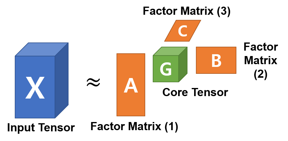
Figure 1: Tucker factorization for a 3-way tensor.

Our proposed method P-Tucker is based on Tucker factorization, one of the most popular decomposition methods. More details about other factorization algorithms are summarized in Section VI and [11].

Definition 4 (Tucker Factorization)

Given an N-order tensor $\boldsymbol{\mathscr{X}}$ $(\in\mathbb{R}^{I_{1}\times...\times I_{N}})$, Tucker factorization approximates $\boldsymbol{\mathscr{X}}$ by a core tensor $\boldsymbol{\mathscr{G}}$ $(\in\mathbb{R}^{J_{1}\times...\times J_{N}})$ and factor matrices $\{\mathbf{A}^{(n)}\in\mathbb{R}^{I_{n}\times J_{n}}|n=1...N\}$. Figure 1 illustrates a Tucker factorization result for a 3-way tensor. Core tensor $\boldsymbol{\mathscr{G}}$ is assumed to be smaller and denser than the input tensor $\boldsymbol{\mathscr{X}}$, and factor matrices $\mathbf{A}^{(n)}$ to be normally orthogonal. Regarding interpretations of factorization results, each factor matrix $\mathbf{A}^{(n)}$ represents the latent features of the object related to the $n$th mode of $\boldsymbol{\mathscr{X}}$, and each element of a core tensor $\boldsymbol{\mathscr{G}}$ indicates the weights of the relations composed of columns of factor matrices. Tucker factorization with tensor operations is presented as follows:

$$\min_{\boldsymbol{\mathscr{G}},\mathbf{A}^{(1)},...,\mathbf{A}^{(N)}}||\boldsymbol{\mathscr{X}}-\boldsymbol{\mathscr{G}}\times_{1}\mathbf{A}^{(1)}\cdots\times_{N}\mathbf{A}^{(N)}||.$$ (3)

Note that the loss function (3) is calculated by all entries of $\boldsymbol{\mathscr{X}}$, and whole missing values of $\boldsymbol{\mathscr{X}}$ are regarded as zeros. Concurrently, an element-wise expression is given as follows:

$$\boldsymbol{\mathscr{X}}_{(i_{1},...,i_{N})}\approx\sum_{\forall{(j_{1},...,j_{N})}\in\boldsymbol{\mathscr{G}}}\boldsymbol{\mathscr{G}}_{(j_{1},...,j_{N})}\prod_{n=1}^{N}a^{(n)}_{i_{n}j_{n}}.$$ (4)

Equation (4) is used to predict values of missing entries after $\boldsymbol{\mathscr{G}},\mathbf{A}^{(1)},...,\mathbf{A}^{(N)}$ are found. We define the reconstruction error of Tucker factorization of $\boldsymbol{\mathscr{X}}$ by the following rule. Note that $\Omega$ is the set of observable entries of $\boldsymbol{\mathscr{X}}$.

$$\footnotesize\sqrt{\sum_{\forall{(i_{1},...,i_{N})}\in\Omega}{\left(\boldsymbol{\mathscr{X}}_{(i_{1},...,i_{N})}-\sum_{\forall{(j_{1},...,j_{N})}\in\boldsymbol{\mathscr{G}}}\boldsymbol{\mathscr{G}}_{(j_{1},...,j_{N})}\prod_{n=1}^{N}a^{(n)}_{i_{n}j_{n}}\right)^{2}}}$$ (5)

Definition 5 (Sparse Tucker Factorization)

Given a tensor $\boldsymbol{\mathscr{X}}~{}(\in\mathbb{R}^{I_{1}\times...\times I_{N}})$ with observable entries $\Omega$, the goal of sparse Tucker factorization of $\boldsymbol{\mathscr{X}}$ is to find factor matrices $\mathbf{A}^{(n)}$ $(\in\mathbb{R}^{I_{n}\times J_{n}},n=1,\cdots,N)$ and a core tensor $\boldsymbol{\mathscr{G}}~{}(\in\mathbb{R}^{J_{1}\times...\times J_{N}})$, which minimize (6).

$$L(\boldsymbol{\mathscr{G}},\mathbf{A}^{(1)},...,\mathbf{A}^{(N)})=\\ \sum_{\forall(i_{1},...,i_{N})\in\Omega}{\left(\boldsymbol{\mathscr{X}}_{(i_{1},...,i_{N})}-\sum_{\forall(j_{1},...,j_{N})\in\boldsymbol{\mathscr{G}}}\boldsymbol{\mathscr{G}}_{(j_{1},...,j_{N})}\prod_{n=1}^{N}a^{(n)}_{i_{n}j_{n}}\right)^{2}}\\ +\lambda\sum_{n=1}^{N}{{\|\mathbf{A}^{(n)}\|}^{2}}$$ (6)

Note that the loss function (6) only depends on observable entries of $\boldsymbol{\mathscr{X}}$, and $L_{2}$ regularization is used in (6) to prevent overfitting, which has been generally utilized in machine learning problems [21, 22, 23].

Definition 6 (Alternating Least Squares)

To minimize the loss functions (3) and (6), an alternating least squares (ALS) technique is widely used [11, 14], which updates a factor matrix or a core tensor while keeping all others fixed.

Input :  Tensor $\boldsymbol{\mathscr{X}}\in\mathbb{R}^{I_{1}\times I_{2}\times\cdots\times I_{N}}$, and

core tensor dimensionality $J_{1},...,J_{N}$.

Output :  Updated factor matrices $\mathbf{A}^{(n)}\in\mathbb{R}^{I_{n}\times J_{n}}$ $(n=1,...,N)$, and

updated core tensor $\boldsymbol{\mathscr{G}}\in\mathbb{R}^{J_{1}\times J_{2}\times\cdots\times J_{N}}$.

1 initialize all factor matrices $\mathbf{A}^{(n)}$

2 repeat

3       for $n=1...N$ do

4             $\boldsymbol{\mathscr{Y}}\leftarrow\boldsymbol{\mathscr{X}}\times_{1}\mathbf{A}^{(1)\mathbf{T}}\cdots\times_{n-1}\mathbf{A}^{(n-1)\mathbf{T}}\times_{n+1}\mathbf{A}^{(n+1)\mathbf{T}}\cdots\times_{N}\mathbf{A}^{(N)\mathbf{T}}$

5             $\mathbf{A}^{(n)}\leftarrow J_{n}$ leading left singular vectors of $\boldsymbol{\mathscr{Y}}_{(n)}$

6      

7until the max. iteration or reconstruction error converges;

$\boldsymbol{\mathscr{G}}\leftarrow\boldsymbol{\mathscr{X}}\times_{1}\mathbf{A}^{(1)\mathsf{T}}\cdots\times_{N}\mathbf{A}^{(N)\mathsf{T}}$

Algorithm 1 Tucker-ALS

Algorithm 1 describes a conventional Tucker factorization based on the ALS, which is called the higher-order orthogonal iteration (HOOI) (see [11] for details). The computational and memory bottleneck of Algorithm 1 is updating factor matrices $\mathbf{A}^{(n)}$ (lines 4-5), which requires tensor operations and SVD. Specifically, Algorithm 1 requires storing a full-dense matrix $\boldsymbol{\mathscr{Y}}_{(n)}$, and the amount of memory needed for storing $\boldsymbol{\mathscr{Y}}_{(n)}$ is $O(I_{n}\prod_{m\neq n}{J_{m}})$. The required memory grows rapidly when the order, the dimensionality, or the rank of a tensor increase, and ultimately causes intermediate data explosion [16]. Moreover, Algorithm 1 computes SVD for a given $\boldsymbol{\mathscr{Y}}_{(n)}$, where the complexity of exact SVD is $O(\min(I_{n}\prod_{m\neq n}{J_{m}^{2}},I_{n}^{2}\prod_{m\neq n}{J_{m}}))$. The computational costs for SVD increase rapidly as well for a large-scale tensor. Notice that Algorithm 1 assumes missing entries of $\boldsymbol{\mathscr{X}}$ as zeros during the update process (lines 4-5), and core tensor $\boldsymbol{\mathscr{G}}$ (line 7) is uniquely determined and relatively easy to be computed by an input tensor and factor matrices.

In summary, applying the naive Tucker-ALS algorithm on sparse tensors generates severe accuracy and scalability issues. Therefore, Algorithm 1 needs to be revised to focus only on observed entries and scale for large-scale tensors at the same time. In that case, an alternative ALS approach is applicable to Algorithm 1, which is utilized for partially observable matrices [23] and CP factorizations [24]. The alternative ALS approach is discussed in Section III.

Definition 7 (Intermediate Data)

We define intermediate data as memory requirements for updating $\mathbf{A}^{(n)}$ (lines 4-5 in Algorithm 1), excluding memory space for storing $\boldsymbol{\mathscr{X}}$, $\boldsymbol{\mathscr{G}}$, and $\mathbf{A}^{(n)}$. The size of intermediate data plays a critical role in determining which Tucker factorization algorithms are space-efficient, as we will discuss in Section III-E2.

III Proposed Method

We describe P-Tucker, our proposed Tucker factorization algorithm for sparse tensors. As described in Definition 6, the computational and memory bottleneck of the standard Tucker-ALS algorithm occurs while updating factor matrices. Therefore, it is imperative to update them efficiently in order to maximize scalability of the algorithm. However, there are several challenges in designing an optimized algorithm for updating factor matrices.

1. Exploit the characteristic of sparse tensors. Sparse tensors are composed of a vast number of missing entries and a small number of observable entries. How can we exploit the sparsity of given tensors to design an accurate and scalable algorithm for updating factor matrices?

2. Maximize scalability. The aforementioned Tucker-ALS algorithm suffers from intermediate data explosion and high computational costs while updating factor matrices. How can we formulate efficient algorithms for updating factor matrices in terms of time and memory?

3. Parallelization. It is crucial to avoid race conditions and adjust workloads between threads to thoroughly employ multi-core parallelism. How can we apply data parallelism on updating factor matrices in order to scale up linearly with respect to the number of threads?

To overcome the above challenges, we suggest the following main ideas, which we describe in later subsections.

1. Row-wise update rule fully exploits the sparsity of a given tensor and enhances the accuracy of a factorization (Figure 3 and Section III-B).

2. P-Tucker-Cache and P-Tucker-Approx accelerate the update process by caching intermediate calculations and truncating “noisy” entries from a core tensor, while P-Tucker itself provides a memory-optimized algorithm by default (Section III-C).

3. Careful distribution of work assures that each thread has independent tasks and balanced workloads when P-Tucker updates factor matrices. (Section III-D).

We first suggest an overview of how P-Tucker factorizes sparse tensors using Tucker method in Section III-A. After that, we describe details of our main ideas in Sections III-B$\thicksim$III-D, and we offer a theoretical analysis of P-Tucker in Section III-E.

III-A Overview

P-Tucker provides an efficient Tucker factorization algorithm for sparse tensors.

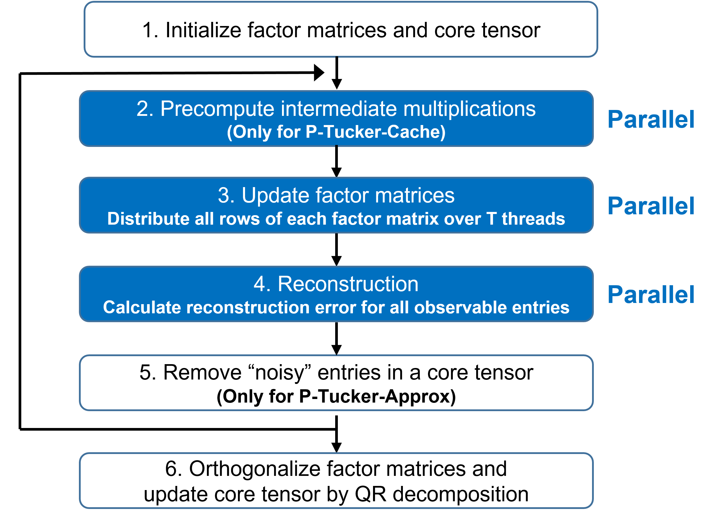
Figure 2: An overview of P-Tucker. After initialization, P-Tucker updates factor matrices in a fully-parallel way. When the reconstruction error converges, P-Tucker performs QR decomposition to make factor matrices orthogonal and updates a core tensor.

Figure 2 and Algorithm 2 describe the main process of P-Tucker. First, P-Tucker initializes all $\mathbf{A}^{(n)}$ and $\boldsymbol{\mathscr{G}}$ with random real values between 0 and 1 (step 1 and line 1). After that, P-Tucker updates factor matrices (steps 2-3 and line 3) by Algorithm 3 explained in Section III-B. When all factor matrices are updated, P-Tucker measures reconstruction error using (5) (step 4 and line 4). In case of P-Tucker-Approx (step 5 and lines 5-6), P-Tucker-Approx removes “noisy” entries of $\boldsymbol{\mathscr{G}}$ by Algorithm 4 explained in Section III-C. P-Tucker stops iterations if the error converges or the maximum iteration is reached (line 7). Finally, P-Tucker performs QR decomposition on all $\mathbf{A}^{(n)}$ to make them orthogonal and updates $\boldsymbol{\mathscr{G}}$ (step 6 and lines 8-11). Specifically, QR decomposition [25] on each $\mathbf{A}^{(n)}$ is defined as follows:

$$\mathbf{A}^{(n)}=\mathbf{Q}^{(n)}\mathbf{R}^{(n)},~{}n=1...N\\$$ (7)

where $\mathbf{Q}^{(n)}\in\mathbb{R}^{I_{n}\times J_{n}}$ is column-wise orthonormal and $\mathbf{R}^{(n)}\in\mathbb{R}^{J_{n}\times J_{n}}$ is upper-triangular. Therefore, by substituting $\mathbf{Q}^{(n)}$ for $\mathbf{A}^{(n)}$, P-Tucker succeeds in making factor matrices orthogonal. Core tensor $\boldsymbol{\mathscr{G}}$ must be updated accordingly in order to maintain the same reconstruction error. According to [26], the update rule of core tensor $\boldsymbol{\mathscr{G}}$ is given as follows:

$$\boldsymbol{\mathscr{G}}\leftarrow\boldsymbol{\mathscr{G}}\times_{1}\mathbf{R}^{(1)}\cdots\times_{N}\mathbf{R}^{(N)}.$$ (8)

Input :  Tensor $\boldsymbol{\mathscr{X}}\in\mathbb{R}^{I_{1}\times I_{2}\times\cdots\times I_{N}}$,

core tensor dimensionality $J_{1},...,J_{N}$, and

truncation rate $p$ (P-Tucker-Approx only).

Output :  Updated factor matrices $\mathbf{A}^{(n)}\in\mathbb{R}^{I_{n}\times J_{n}}(n=1,...,N)$,

and updated core tensor $\boldsymbol{\mathscr{G}}\in\mathbb{R}^{J_{1}\times J_{2}\times\cdots\times J_{N}}$.

1 initialize factor matrices $\mathbf{A^{(n)}}~{}(n=1,...,N)$ and core tensor $\boldsymbol{\mathscr{G}}$

2 repeat

3       update factor matrices $\mathbf{A}^{(n)}~{}(n=1,...,N)$ by Algorithm 3

4       calculate reconstruction error using (5)

5       if P-Tucker-Approx then $\triangleright$ $\boldsymbol{\mathscr{G}}$ Truncation

6             remove “noisy” entries of $\boldsymbol{\mathscr{G}}$ by Algorithm 4

7      

8until the maximum iteration or $\|\boldsymbol{\mathscr{X}}-\boldsymbol{\mathscr{X^{\prime}}}\|$ converges;

9for n = 1…$N$ do

10       $\mathbf{A}^{(n)}\rightarrow\mathbf{Q}^{(n)}\mathbf{R}^{(n)}$ $\triangleright$ QR decomposition

11       $\mathbf{A}^{(n)}\leftarrow\mathbf{Q}^{(n)}$ $\triangleright$ Orthogonalize $\mathbf{A}^{(n)}$

12       $\boldsymbol{\mathscr{G}}\leftarrow\boldsymbol{\mathscr{G}}\times_{n}\mathbf{R}^{(n)}$ $\triangleright$ Update core tensor $\boldsymbol{\mathscr{G}}$

Algorithm 2 P-Tucker for Sparse Tensors

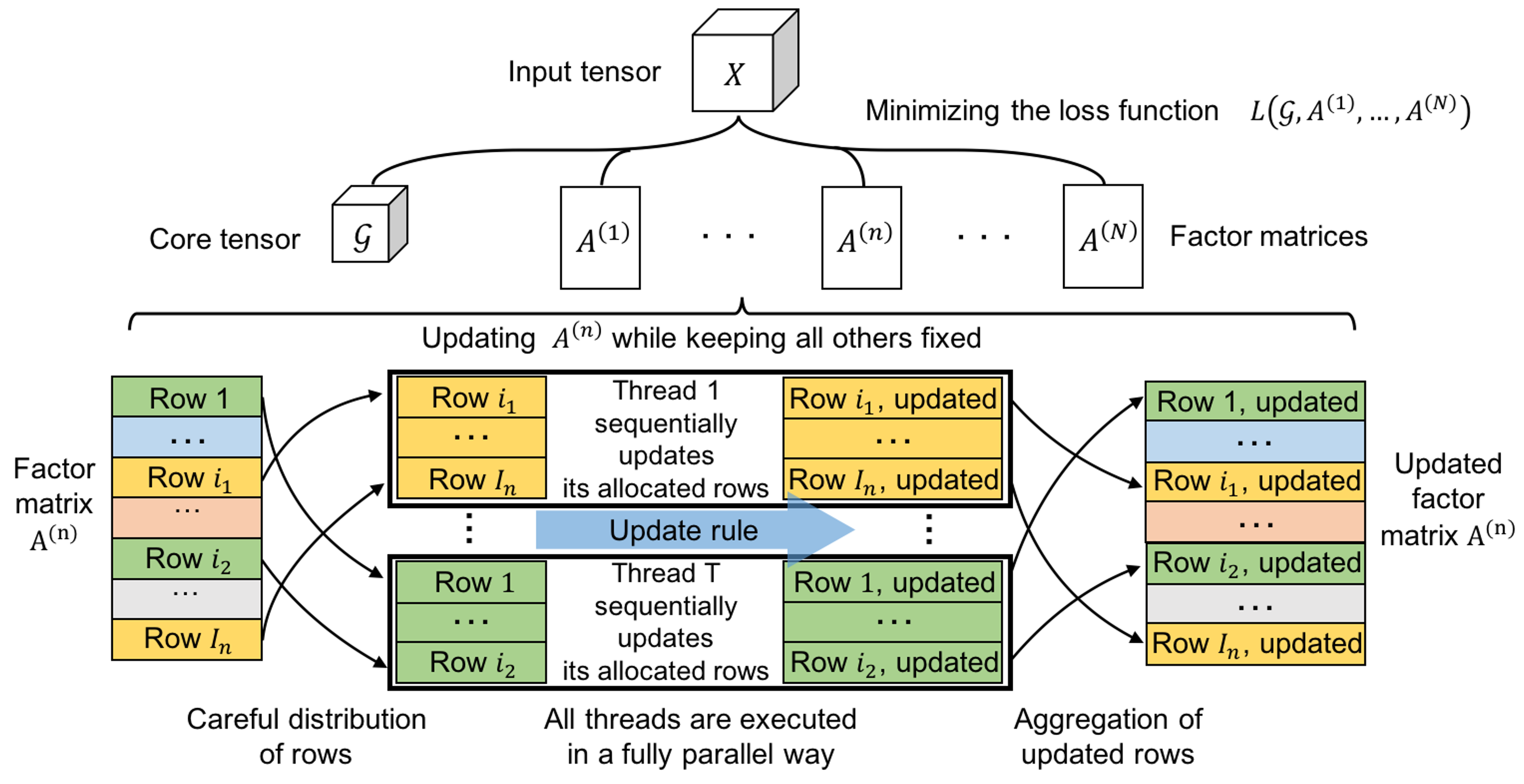
Figure 3: An overview of updating factor matrices. P-Tucker performs a row-wise ALS which updates each row of a factor matrix $\mathbf{A}^{(n)}$ while keeping all the others fixed. Since all rows of a factor matrix are independent of each other in terms of minimizing the loss function (6), P-Tucker fully exploits multi-core parallelism to update all rows of $\mathbf{A}^{(n)}$. First, all rows are carefully distributed to all threads to achieve a uniform workload among them. After that, all threads update their allocated rows in a fully parallel way. In a single thread, the allocated rows are updated in a sequential way. Finally, P-Tucker aggregates all updated rows from all threads to update $\mathbf{A}^{(n)}$. P-Tucker iterates this update procedure for all factor matrices one by one.

III-B Row-wise Updates of Factor Matrices

P-Tucker updates factor matrices in a row-wise manner based on ALS, where an update rule for a row is computed by only observed entries of a tensor. From a high-level point of view, as most ALS methods do, P-Tucker updates a factor matrix at a time while maintaining all others fixed. However, when all other matrices are fixed, there are several approaches [24] for updating a single factor matrix. Among them, P-Tucker selects a row-wise update method; a key benefit of the row-wise update is that all rows of a factor matrix are independent of each other in terms of minimizing the loss function (6). This property enables applying multi-core parallelism on updating factor matrices. Given a row of a factor matrix, an update rule is derived by computing a gradient with respect to the given row and setting it as zero, which minimizes the loss function (6). The update rule for the $i_{n}$th row of the $n$th factor matrix $\mathbf{A}^{(n)}$ (see Figure 4) is given as follows; the proof of Equation (9) is in Theorem 1.

$$\begin{aligned} \leftarrow\underset{[a^{(n)}_{i_{n}1},...,a^{(n)}_{i_{n}J_{n}}]}{\operatorname{arg}\,\operatorname{min}}\;{L(\boldsymbol{\mathscr{G}},\mathbf{A}^{(1)},...,\mathbf{A}^{(N)})}\\ =\mathbf{c}_{i_{n}:}^{(n)}\times[\mathbf{B}_{i_{n}}^{(n)}+\lambda\mathbf{I}_{J_{n}}]^{-1}\end{aligned}$$ (9)

where $\mathbf{B}_{i_{n}}^{(n)}$ is a ${J_{n}\times J_{n}}$ matrix whose $(j_{1},j_{2})$th entry is

$$\sum_{\forall(i_{1},...,i_{N})\in\Omega_{i_{n}}^{(n)}}\delta_{(i_{1},...,i_{N})}^{(n)}(j_{1})\delta_{(i_{1},...,i_{N})}^{(n)}(j_{2}),$$ (10)

$\mathbf{c}_{i_{n}:}^{(n)}$ is a length ${J_{n}}$ vector whose $j$th entry is

$$\sum_{\forall(i_{1},...,i_{N})\in\Omega_{i_{n}}^{(n)}}\boldsymbol{\mathscr{X}}_{(i_{1},...,i_{N})}\delta_{(i_{1},...,i_{N})}^{(n)}(j),$$ (11)

$\delta_{(i_{1},...,i_{N})}^{(n)}$ is a length ${J_{n}}$ vector whose $j$th entry is

$$\sum_{\forall(j_{1}...j_{n}=j...j_{N})\in\boldsymbol{\mathscr{G}}}\boldsymbol{\mathscr{G}}_{(j_{1}...j_{n}=j...j_{N})}\prod_{k\neq n}a^{(k)}_{i_{k}j_{k}},$$ (12)

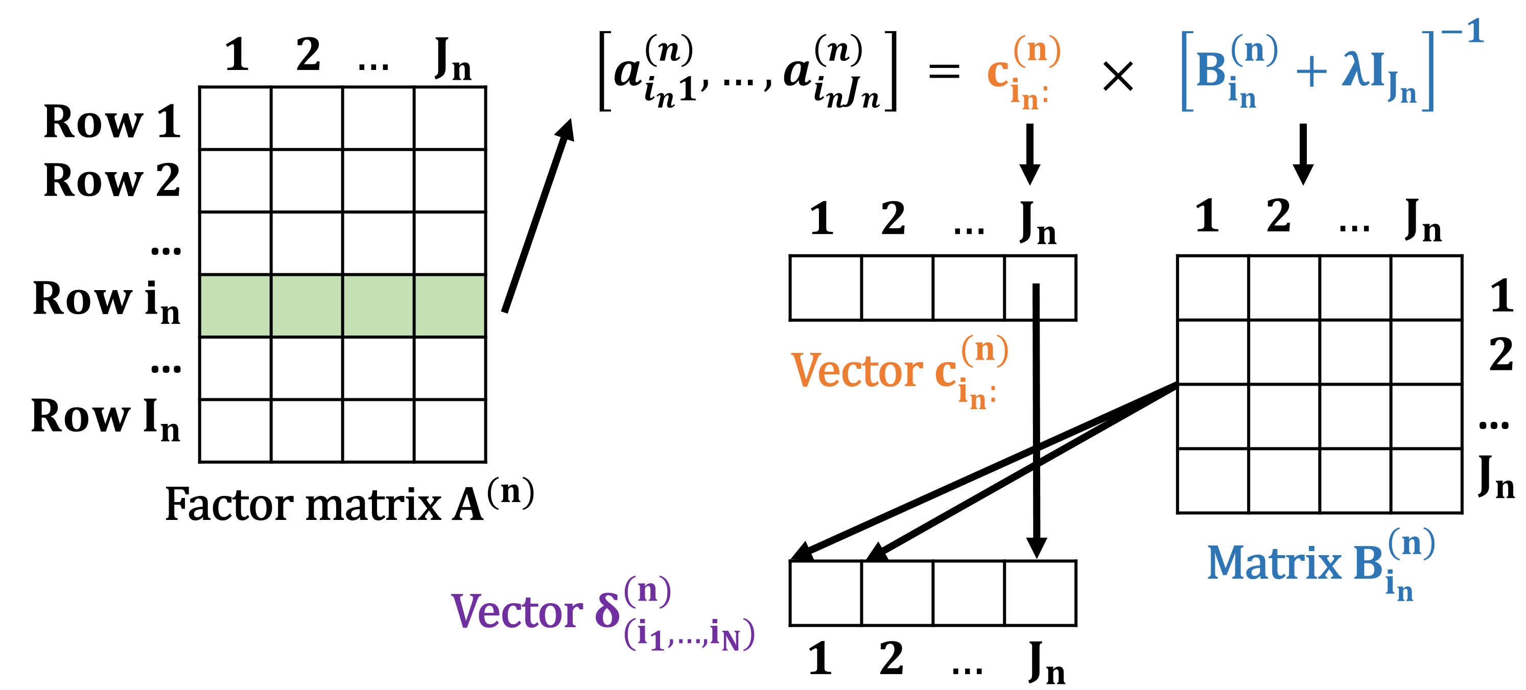
Figure 4: An illustration of an update rule for a row of a factor matrix. P-Tucker requires three intermediate data $\mathbf{B}_{i_{n}}^{(n)}$, $\mathbf{c}_{i_{n}:}^{(n)}$, and $\delta_{(i_{1},...,i_{N})}^{(n)}$ for updating the $i_{n}$th row of $\mathbf{A^{(n)}}$. Note that $\lambda$ is a regularization parameter, and $\mathbf{I}_{J_{n}}$ is a $J_{n}\times J_{n}$ identity matrix.

$\Omega_{i_{n}}^{(n)}$ indicates the subset of $\Omega$ whose $n$th mode’s index is $i_{n}$, $\lambda$ is a regularization parameter, and $\mathbf{I}_{J_{n}}$ is a $J_{n}\times J_{n}$ identity matrix. As shown in Figure 4, the update rule for the $i_{n}$th row of $\mathbf{A}^{(n)}$ requires three intermediate data $\mathbf{B}_{i_{n}}^{(n)}$, $\mathbf{c}_{i_{n}:}^{(n)}$, and $\delta_{(i_{1},...,i_{N})}^{(n)}$. Those data are computed by the subset of observable entries $\Omega_{i_{n}}^{(n)}$. Thus, computational costs of updating factor matrices are proportional to the number of observable entries, which lets P-Tucker fully exploit the sparsity of given tensors. Moreover, P-Tucker predicts missing values of a tensor using (4), not as zeros. Equation (4) is computed by updated factor matrices and a core tensor, and they are learned by observed entries of a tensor. Hence, P-Tucker not only enhances the accuracy of factorizations, but also reflects the latent-characteristics of observed entries of a tensor. Note that a matrix $[\mathbf{B}_{i_{n}}^{(n)}+\lambda\mathbf{I}_{J_{n}}]$ is positive-definite and invertible, and a proof of the update rule is summarized in Section III-E1.

Input :  Tensor $\boldsymbol{\mathscr{X}}\in\mathbb{R}^{I_{1}\times I_{2}\times\cdots\times I_{N}}$,

factor matrices $\mathbf{A}^{(n)}\in\mathbb{R}^{I_{n}\times J_{n}}~{}(n=1,...,N)$,

core tensor $\boldsymbol{\mathscr{G}}\in\mathbb{R}^{J_{1}\times J_{2}\times\cdots\times J_{N}}$ , and

cache table $Pres\in\mathbb{R}^{|\Omega|\times|\boldsymbol{\mathscr{G}}|}$ (P-Tucker-Cache only).

Output :  Updated factor matrices $\mathbf{A}^{(n)}\in\mathbb{R}^{I_{n}\times J_{n}}~{}(n=1,...,N)$.

1 if P-Tucker-Cache then $\triangleright$ Precompute $Pres$

2       for ${\alpha=\forall(i_{1},...,i_{N})}\in\Omega$ do $\triangleright$ In parallel

3             for ${\beta=\forall(j_{1},...,j_{N})}\in\boldsymbol{\mathscr{G}}$ do

4                   $Pres[\alpha][\beta]\leftarrow\boldsymbol{\mathscr{G}}_{\beta}\prod_{k=1}^{N}{a_{i_{k}j_{k}}^{(k)}}$

5            

6      

7for n = 1…$N$ do $\triangleright$ nth factor matrix

8       for $i_{n}$ = 1…$I_{n}$ do $\triangleright$ $i_{n}$th row, in parallel

9             for $\alpha=\forall(i_{1},...,i_{N})\in\Omega_{i_{n}}^{(n)}$ do

10                   for $\beta=\forall(j_{1},...,j_{N})\in\boldsymbol{\mathscr{G}}$ do $\triangleright$ Compute $\delta$

11                         if P-Tucker then

12                               $\delta_{\alpha}^{(n)}(j_{n})\leftarrow\delta_{\alpha}^{(n)}(j_{n})+\boldsymbol{\mathscr{G}}_{\beta}\prod_{k\neq n}a_{i_{k}j_{k}}^{(k)}$

13                              

14                        if P-Tucker-Cache then

15                               $\delta_{\alpha}^{(n)}(j_{n})\leftarrow\delta_{\alpha}^{(n)}(j_{n})+\frac{Pres[\alpha][\beta]}{a_{i_{n}j_{n}}^{(n)}}$

16                              

17                        

18                  calculate $\mathbf{B}_{i_{n}}^{(n)}$ and $\mathbf{c}_{i_{n}:}^{(n)}$ using (10) and (11)

19                  

20            find the inverse matrix of $[\mathbf{B}_{i_{n}}^{(n)}+\lambda\mathbf{I}_{J_{n}}]$

21             update $[a_{i_{n}1}^{(n)},\cdots,a_{i_{n}J_{n}}^{(n)}]$ using (9)

22      if P-Tucker-Cache then $\triangleright$ Update $Pres$

23             for $\alpha=\forall(i_{1},...,i_{N})\in\Omega$ do $\triangleright$ In parallel

24                   for $\beta=\forall(j_{1},...,j_{N})\in\boldsymbol{\mathscr{G}}$ do

25                         $Pres[\alpha][\beta]\leftarrow\frac{Pres[\alpha][\beta]}{(a,old)_{i_{n}j_{n}}^{(n)}}\times(a,new)_{i_{n}j_{n}}^{(n)}$

26                  

27            

28      

Algorithm 3 P-Tucker for Updating Factor Matrices

Algorithm 3 describes how P-Tucker updates factor matrices. First, in case of P-Tucker-Cache (lines 1-4), it computes the values of all entries in a cache table $Pres$ $(\in\mathbb{R}^{|\Omega|\times|\boldsymbol{\mathscr{G}}|})$ which caches intermediate multiplication results generated while updating factor matrices. This memoization technique allows P-Tucker-Cache to be a time-efficient algorithm. Next, P-Tucker chooses a row $\mathbf{a}_{i_{n}:}^{(n)}$ of a factor matrix $\mathbf{A}^{(n)}$ to update (lines 5-6). After that, P-Tucker computes $\mathbf{B}_{i_{n}}^{(n)}$ and $\mathbf{c}_{i_{n}:}^{(n)}$ required for updating a row $\mathbf{a}_{i_{n}:}^{(n)}$ (lines 7-13). P-Tucker performs matrix inverse operation on $[\mathbf{B}_{i_{n}}^{(n)}+\lambda\mathbf{I}_{J_{n}}]$ (line 14) and updates a row $\mathbf{a}_{i_{n}:}^{(n)}$ by the multiplication of $\mathbf{c}_{i_{n}:}^{(n)}$ and $[\mathbf{B}_{i_{n}}^{(n)}+\lambda\mathbf{I}_{J_{n}}]^{-1}$ (line 15). In case of P-Tucker-Cache, it recalculates $Pres$ using the existing and updated $\mathbf{A}^{(n)}$ (lines 16-19) whenever $\mathbf{A}^{(n)}$ is updated. Note that $\alpha$ and $\beta$ indicate an entry of $\boldsymbol{\mathscr{X}}$ and $\boldsymbol{\mathscr{G}}$, respectively.

III-C Variants: P-Tucker-Cache and P-Tucker-Approx

As discussed in Section III-B, P-Tucker requires three intermediate data: $\mathbf{B}_{i_{n}}^{(n)}$, $\mathbf{c}_{i_{n}:}^{(n)}$, and $\delta_{(i_{1},...,i_{N})}^{(n)}$ whose memory requirements are $O(J_{n}^{2})$. Considering the memory complexity of the naive Tucker-ALS, which is $O(I_{n}\prod_{m\neq n}{J_{m}})$, P-Tucker successfully provides a memory-optimized algorithm. We can further optimize P-Tucker in terms of time by a caching algorithm (P-Tucker-Cache) and an approximation algorithm (P-Tucker-Approx).

The crucial difference between P-Tucker and P-Tucker-Cache lies in the computation of the intermediate vector $\delta$ (lines 9-12 in Algorithm 3). In case of P-Tucker, updating $\delta$ requires $N$ times of multiplications for a given entry pair $(\alpha,\beta)$ (line 10), which takes $O(N)$. However, if we cache the results of those multiplications for all entry pairs, the update only takes $O(1)$ (line 12). This trade-off distinguishes P-Tucker-Cache and P-Tucker. P-Tucker-Cache accelerates intermediate calculations by the memoization technique with the cache table $Pres$. Meanwhile, P-Tucker requires only small vectors $\mathbf{c}_{i_{n}:}^{(n)}$ and $\delta_{(i_{1},...,i_{N})}^{(n)}$ ($\in\mathbb{R}^{J_{n}}$) and a small matrix $\mathbf{B}_{i_{n}}^{(n)}$ ($\in\mathbb{R}^{J_{n}\times J_{n}}$) as intermediate data. Note that when $a_{i_{n}j_{n}}^{(n)}$ is 0 (lines 12 and 19), P-Tucker-Cache conducts the multiplications as P-Tucker does (line 10).

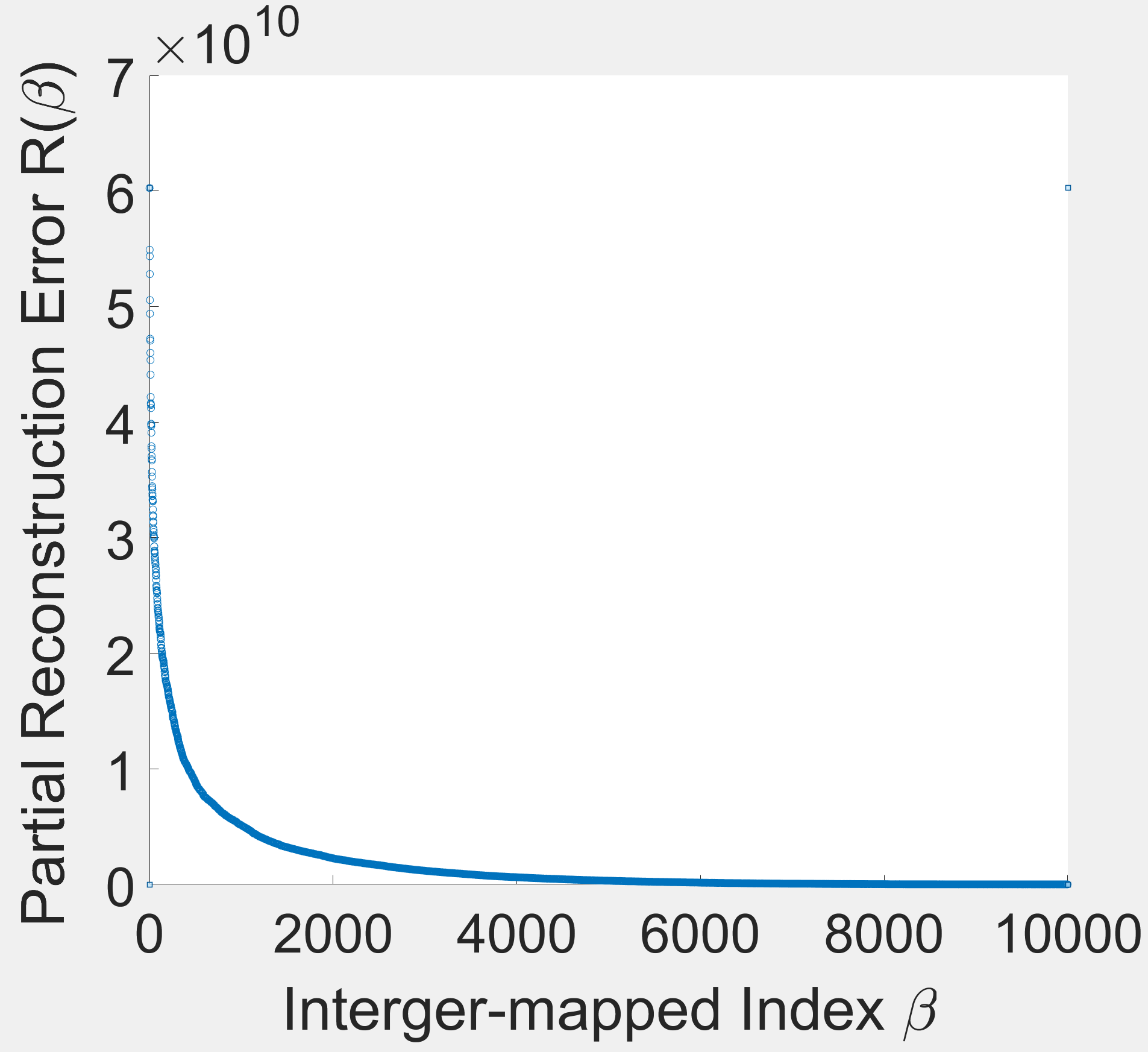
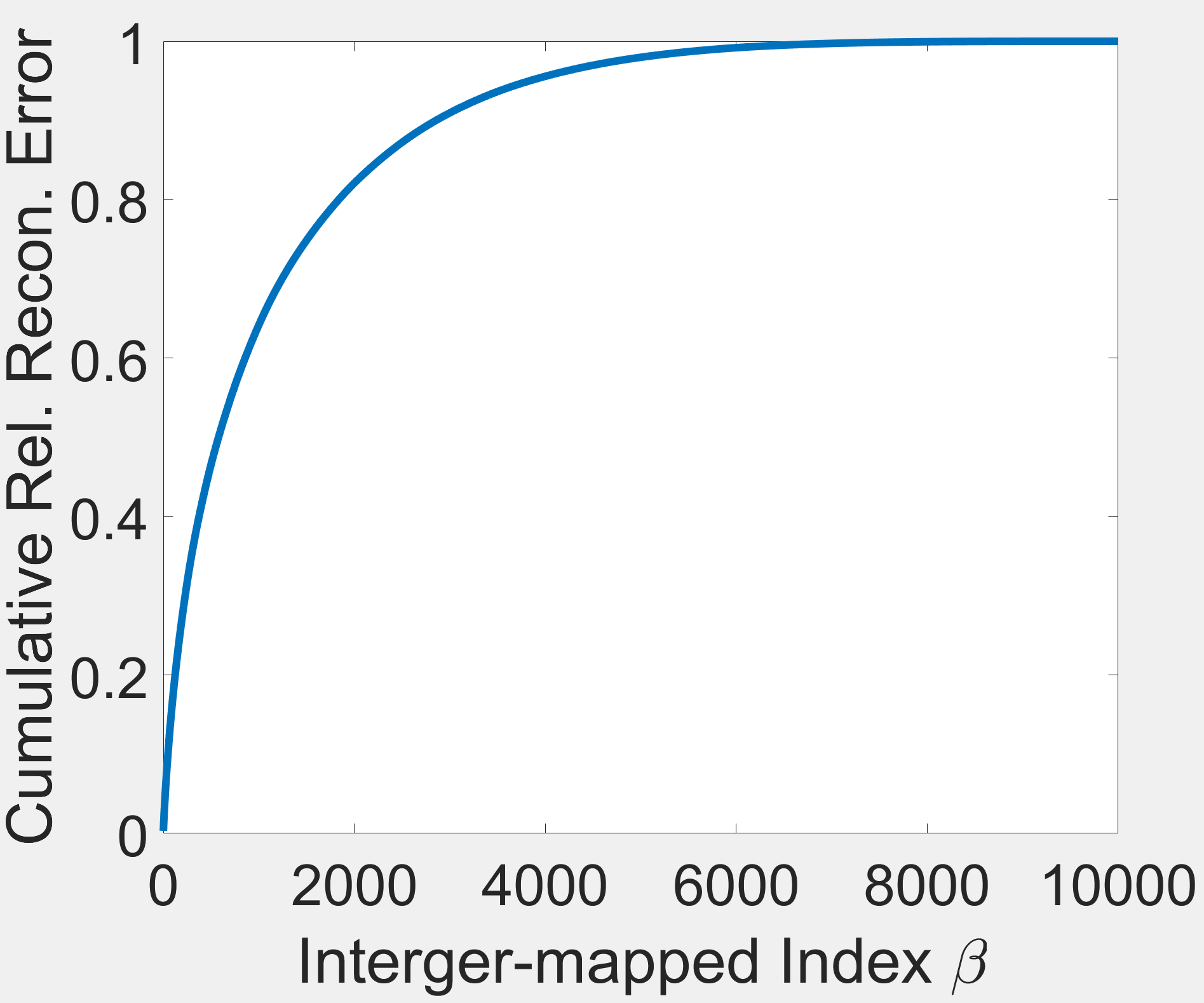
Figure 5: Distribution of partial reconstruction error $\boldsymbol{\mathscr{R}}(\beta)$ and accumulation of relative reconstruction error produced by an entry $\beta=(j_{1},...,j_{N})$ of a core tensor $\boldsymbol{\mathscr{G}}$. Note that 20% “noisy“ entries of $\boldsymbol{\mathscr{G}}$ generate 80% of total reconstruction error.

The main intuition of P-Tucker-Approx is that there exist “noisy” entries in a core tensor $\boldsymbol{\mathscr{G}}$, and we can accelerate the update process by truncating these “noisy” entries of $\boldsymbol{\mathscr{G}}$. Then, how can we determine whether an entry of $\boldsymbol{\mathscr{G}}$ is “noisy” or not? A naive approach could be treating an entry $(j_{1},...,j_{N})\in\boldsymbol{\mathscr{G}}$ with small $\boldsymbol{\mathscr{G}}_{(j_{1},...,j_{N})}$ value as ”noisy” like the truncated SVD [27]. However, in this case, small-value entries are not always negligible since their contributions to minimizing the error (5) can be larger than that of large-value ones. Hence, we propose more precise criterion which regards an entry $\beta=(j_{1},...,j_{N})\in\boldsymbol{\mathscr{G}}$ with a high $\boldsymbol{\mathscr{R}}(\beta)$ value as “noisy”. $\boldsymbol{\mathscr{R}}(\beta)$ indicates a partial reconstruction error produced by an entry $\beta$, derived from the sum of terms only related to $\beta$ in (5). Given an entry $\beta=(j_{1},...,j_{N})\in\boldsymbol{\mathscr{G}}$, $\boldsymbol{\mathscr{R}}(\beta)$ is given as follows:

$$\footnotesize\sum_{\forall{\alpha}\in\Omega}\Bigg{(}{\bigg{(}\boldsymbol{\mathscr{X}}_{\alpha}-\sum_{\forall{\gamma}\in\boldsymbol{\mathscr{G}}}\boldsymbol{\mathscr{G}}_{\gamma}\prod_{n=1}^{N}a^{(n)}_{i_{n}j_{n}}\bigg{)}^{2}}-~{}{\bigg{(}\boldsymbol{\mathscr{X}}_{\alpha}-\sum_{\forall{\gamma}\neq\beta}\boldsymbol{\mathscr{G}}_{\gamma}\prod_{n=1}^{N}a^{(n)}_{i_{n}j_{n}}\bigg{)}^{2}}\Bigg{)}=\\ \footnotesize\sum_{\forall{\alpha}\in\Omega}{(\boldsymbol{\mathscr{G}}_{\beta}\prod_{n=1}^{N}a^{(n)}_{i_{n}j_{n}})\left(-2\boldsymbol{\mathscr{X}}_{\alpha}+\boldsymbol{\mathscr{G}}_{\beta}\prod_{n=1}^{N}a^{(n)}_{i_{n}j_{n}}+2\sum_{\forall{\gamma}\neq\beta}\boldsymbol{\mathscr{G}}_{\gamma}\prod_{n=1}^{N}a^{(n)}_{i_{n}j_{n}}\right)}.$$ (13)

Note that we use $\alpha$, $\beta$, and $\gamma$ symbols to simplify the equation. $\boldsymbol{\mathscr{R}}(\beta)$ suggests a more precise guideline of “noisy” entries since $\boldsymbol{\mathscr{R}}(\beta)$ is a part of (5), while the naive approach assumes the error based on the value $\boldsymbol{\mathscr{G}}_{(j_{1},...,j_{N})}$. Figure 5 illustrates a distribution of $\boldsymbol{\mathscr{R}}(\beta)$ and a cumulative function of relative reconstruction error on the latest MovieLens dataset ($J=10$). As expected by our intuition, only 20% entries of $\boldsymbol{\mathscr{G}}$ generate about 80% of total reconstruction error. Algorithm 4 describes how P-Tucker-Approx truncates “noisy” entries in $\boldsymbol{\mathscr{G}}$. It first computes $\boldsymbol{\mathscr{R}}(\beta)$ (lines 1-2) for all entries in $\boldsymbol{\mathscr{G}}$, and sort $\boldsymbol{\mathscr{R}}(\beta)$ in descending order (line 3) as well as their indices. Finally, it truncates top-$p|\boldsymbol{\mathscr{G}}|$ “noisy” entries of $\boldsymbol{\mathscr{G}}$ (line 4). P-Tucker-Approx performs Algorithm 4 for each iteration (lines 3-6 in Algorithm 2), which reduces the number of non-zeros in $\boldsymbol{\mathscr{G}}$ step-by-step. Therefore, the elapsed time per iteration also decreases since the time complexity of P-Tucker-Approx depends on the number of non-zeros $|\boldsymbol{\mathscr{G}}|$. Practically, we note that P-Tucker-Approx may require few iterations to run faster than P-Tucker due to overheads from calculating $\boldsymbol{\mathscr{R}}(\beta)$, which is computed for all iterations.

Input :  Tensor $\boldsymbol{\mathscr{X}}\in\mathbb{R}^{I_{1}\times I_{2}\times\cdots\times I_{N}}$,

factor matrices $\mathbf{A}^{(n)}\in\mathbb{R}^{I_{n}\times J_{n}}(n=1,...,N)$,

core tensor $\boldsymbol{\mathscr{G}}\in\mathbb{R}^{J_{1}\times J_{2}\times\cdots\times J_{N}}$, and

truncation rate $p~{}(0<p<1).$

Output :  Truncated core tensor $\boldsymbol{\mathscr{G^{\prime}}}\in\mathbb{R}^{J_{1}\times J_{2}\times\cdots\times J_{N}}$.

1 for $\beta=\forall(j_{1},...,j_{N})\in\boldsymbol{\mathscr{G}}$ do

2       compute a partial reconstruction error $\boldsymbol{\mathscr{R}}(\beta)$ by (13)

3sort $\boldsymbol{\mathscr{R}}(\beta)$ in descending order with their indices

remove $p|\boldsymbol{\mathscr{G}}|$ entries in $\boldsymbol{\mathscr{G}}$, whose $\boldsymbol{\mathscr{R}}(\beta)$ value are ranked within top-$p|\boldsymbol{\mathscr{G}}|$ among all $\boldsymbol{\mathscr{R}}(\beta)$ values.

Algorithm 4 Removing noisy entries of a core tensor $\boldsymbol{\mathscr{G}}$ in P-Tucker-Approx

With the above optimizations, P-Tucker becomes the most time and memory efficient method in theoretical and experimental perspectives (see Table III).

III-D Careful Distribution of Work

There are three sections where multi-core parallelization is applicable in Algorithms 2 and 3. The first section (lines 2-4 and 17-19 in Algorithm 3) is for P-Tucker-Cache when it computes and updates the cache table $Pres$. The second section (lines 6-15 in Algorithm 3) is for updating factor matrices, and the last section (line 4 in Algorithm 2) is for measuring the reconstruction error. For each section, P-Tucker carefully distributes tasks to threads while maintaining the independence between them. Furthermore, P-Tucker utilizes a dynamic scheduling method [28] to assure that each thread has balanced workloads, which directly affects the performance (see Section IV-D). The details of how P-Tucker parallelizes each section are as follows. Note that $T$ indicates the number of threads used for parallelization.

• Section 1: Computing and Updating Cache Table $Pres$ (Only for P-Tucker-Cache). All rows of $Pres$ are independent of each other when they are computed or updated. Thus, P-Tucker distributes all rows equally over $T$ threads, and each thread computes or updates allocated rows independently using static scheduling.

• Section 2: Updating Factor Matrices. All rows of $\mathbf{A}^{(n)}$ are independent of each other regarding minimizing the loss function (6). Therefore, P-Tucker distributes all rows uniformly to each thread, and updates them in parallel. Since $|\Omega_{i_{n}}^{(n)}|$ differs for each row, the workload of each thread may vary considerably. Thus, P-Tucker employs dynamic scheduling in this part.

• Section 3: Calculating Reconstruction Error. All observable entries are independent of each other in measuring the reconstruction error. Thus, P-Tucker distributes them evenly over $T$ threads, and each thread computes the error separately using static scheduling. At the end, P-Tucker aggregates the partial error from each thread.

III-E Theoretical Analysis

III-E1 Convergence Analysis

We theoretically prove the correctness and the convergence of P-Tucker.

Theorem 1 (Correctness of P-Tucker)

The proposed row-wise update rule (14) minimizes the loss function (6) regarding the updated parameters.

$$\underset{[a^{(n)}_{i_{n}1},...,a^{(n)}_{i_{n}J_{n}}]}{\operatorname{arg}\,\operatorname{min}}\;{L(\boldsymbol{\mathscr{G}},\mathbf{A}^{(1)},...,\mathbf{A}^{(N)})}=\mathbf{c}_{i_{n}:}^{(n)}\times[\mathbf{B}_{i_{n}}^{(n)}+\lambda\mathbf{I}_{J_{n}}]^{-1}$$ (14)

Proof 1

$$\frac{\partial L}{\partial a_{i_{n}j_{n}}^{(n)}}=0,\forall{j_{n}},1\leq j_{n}\leq J_{n}\quad$$

$$\Leftrightarrow\sum_{\forall{\alpha}\in\Omega_{i_{n}}^{(n)}}\Bigg{(}\bigg{(}\boldsymbol{\mathscr{X}}_{\alpha}-\sum_{\forall{\beta}\in\boldsymbol{\mathscr{G}}}\boldsymbol{\mathscr{G}}_{\beta}\prod_{n=1}^{N}a^{(n)}_{i_{n}j_{n}}\bigg{)}\times\bigg{(}-\delta_{\alpha}^{(n)}(j_{n})\bigg{)}\Bigg{)}+\lambda a_{i_{n}j_{n}}^{(n)}=0$$

$$\Leftrightarrow[a^{(n)}_{i_{n}1},...,a^{(n)}_{i_{n}J_{n}}]\Bigg{(}\sum_{\forall{\alpha}\in\Omega_{i_{n}}^{(n)}}\bigg{(}\delta_{\alpha}^{(n)\mathbf{T}}\delta_{\alpha}^{(n)}\bigg{)}+\lambda\mathbf{I}_{J_{n}}\Bigg{)}=\sum_{\forall{\alpha}\in\Omega_{i_{n}}^{(n)}}\Bigg{(}\boldsymbol{\mathscr{X}}_{\alpha}\delta_{\alpha}^{(n)}\Bigg{)}$$

$$\Leftrightarrow[a^{(n)}_{i_{n}1},...,a^{(n)}_{i_{n}J_{n}}]=\mathbf{c}_{i_{n}:}^{(n)}\times[\mathbf{B}_{i_{n}}^{(n)}+\lambda\mathbf{I}_{J_{n}}]^{-1}$$

Note that the full proof of Theorem 1 is in the supplementary material of P-Tucker [29].

Theorem 2 (Convergence of P-Tucker)

P-Tucker converges since (6) is bounded and decreases monotonically.

Proof 2

According to Theorem 1, the loss function (6) never increases since every update in P-Tucker minimizes it, and (6) is bounded by 0. Thus, P-Tucker converges.

TABLE III: Complexity analysis of P-Tucker and other methods with respect to time and memory. The optimal complexities are in bold. P-Tucker and its variants exhibit the best time and memory complexity among all methods. Note that memory complexity indicates the space requirement for intermediate data.

Algorithm	Time Complexity	Memory
	(per iteration)	Complexity
P-Tucker	$O(NIJ^{3}+N^{2}|\Omega|J^{N})$	$\mathbf{O(TJ^{2})}$
P-Tucker-Cache	$O(NIJ^{3}+N|\Omega|J^{N})$	$O(|\Omega|J^{N})$
P-Tucker-Approx	$\mathbf{O(NIJ^{3}+N^{2}|\Omega||\boldsymbol{\mathscr{G}}|)}$	$O(J^{N})$
Tucker-wOpt [18]	$O(N\sum_{k=0}^{k=N}(I^{N-k}J^{k}))$	$O(I^{N-1}J)$
Tucker-CSF [20]	$O(NJ^{N-1}(|\Omega|+J^{2(N-1)}))$	$O(IJ^{N-1})$
$\text{S-HOT}_{\text{scan}}$ [17]	$O(NJ^{N}+N|\Omega|J^{N})$	$O(J^{N-1})$

III-E2 Complexity Analysis

We analyze time and memory complexities of P-Tucker and its variants. For simplicity, we assume $I_{1}=...=I_{N}=I$ and $J_{1}=...=J_{N}=J$. Table III summarizes the time and memory complexities of P-Tucker and other methods. As expected in Section III-C, P-Tucker presents the best memory complexity among all algorithms. While P-Tucker-Cache shows better time complexity than that of P-Tucker, P-Tucker-Approx exhibits the best time complexity thanks to the reduced number of non-zeros in $\boldsymbol{\mathscr{G}}$. Note that we calculate time complexities per iteration (lines 3-6 in Algorithm 2), and we focus on memory complexities of intermediate data, not of all variables.

Theorem 3 (Time complexity of P-Tucker)

The time complexity of P-Tucker is $O(NIJ^{3}+N^{2}|\Omega|J^{N})$.

Proof 3

Given the $i_{n}$th row of $\mathbf{A}^{(n)}$ (lines 5-6) in Algorithm 3 , computing $\delta_{\alpha}^{(n)}(j_{n})$ (line 10) takes $O(N|\Omega_{i_{n}}^{(n)}|J^{N})$. Updating $\mathbf{B}_{i_{n}}^{(n)}$ and $\mathbf{c}_{i_{n}:}^{(n)}$ (line 13) takes $O(|\Omega_{i_{n}}^{(n)}|J^{2})$ since $\delta_{\alpha}^{(n)}$ is already calculated. Inverting $[\mathbf{B}_{i_{n}}^{(n)}+\lambda\mathbf{I}_{J_{n}}]$ (line 14) takes $O(J^{3})$, and updating a row (line 15) takes $O(J^{2})$. Thus, the time complexity of updating the $i_{n}$th row of $\mathbf{A}^{(n)}$ (lines 7-15) is $O(J^{3}+N|\Omega_{i_{n}}^{(n)}|J^{N})$. Iterating it for all rows of $\mathbf{A}^{(n)}$ takes $O(IJ^{3}+N|\Omega|J^{N})$. Finally, updating all $\mathbf{A}^{(n)}$ takes $O(NIJ^{3}+N^{2}|\Omega|J^{N})$. According to (5), reconstruction (line 4 in Algorithm 2) takes $O(N|\Omega|J^{N})$. Thus, the time complexity of P-Tucker is $O(NIJ^{3}+N^{2}|\Omega|J^{N})$.

Theorem 4 (Memory complexity of P-Tucker)

The memory complexity of P-Tucker is $O(TJ^{2})$.

Proof 4

The intermediate data of P-Tucker consist of two vectors $\delta_{\alpha}^{(n)}$ and $\mathbf{c}_{i_{n}:}^{(n)}$ ($\in\mathbb{R}^{J}$) , and two matrices $\mathbf{B}_{i_{n}}^{(n)}$ and $[\mathbf{B}_{i_{n}}^{(n)}+\lambda\mathbf{I}_{J_{n}}]^{-1}$ ($\in\mathbb{R}^{J\times J}$). Memory spaces for those variables are released after updating the $i_{n}$th row of $\mathbf{A}^{(n)}$. Thus, they are not accumulated during the iterations. Since each thread has their own intermediate data, the total memory complexity of P-Tucker is $O(TJ^{2})$.

Theorem 5 (Time complexity of P-Tucker-Cache)

The time complexity of P-Tucker-Cache is $O(NIJ^{3}+N|\Omega|J^{N})$.

Proof 5

In Algorithm 3, computing $\delta$ (line 12) takes $O(N|\Omega|J^{N})$ by the caching method. Precomputing and updating $Pres$ (lines 2-4 and 17-19) also take $O(N|\Omega|J^{N})$. Since all the other parts of P-Tucker-Cache are equal to those of P-Tucker, the time complexity of P-Tucker-Cache is $O(NIJ^{3}+N|\Omega|J^{N})$.

Theorem 6 (Memory complexity of P-Tucker-Cache)

The memory complexity of P-Tucker-Cache is $O(|\Omega|J^{N})$.

Proof 6

The cache table $Pres$ requires $O(|\Omega|J^{N})$ memory space, which is much larger than that of other intermediate data (see Theorem 4). Thus, the memory complexity of P-Tucker-Cache is $O(|\Omega|J^{N})$.

Theorem 7 (Time complexity of P-Tucker-Approx)

The time complexity of P-Tucker-Approx is $O(NIJ^{3}+N^{2}|\Omega||\boldsymbol{\mathscr{G}}|)$.

Proof 7

Refer to the supplementary material [29].

Theorem 8 (Memory complexity of P-Tucker-Approx)

The memory complexity of P-Tucker-Approx is $O(J^{N})$.

Proof 8

Refer to the supplementary material [29].

IV Experiments

We present experimental results to answer the following questions.

1. Data Scalability (Section IV-B). How well do P-Tucker and competitors scale up with respect to the following aspects of a given tensor: 1) the order, 2) the dimensionality, 3) the number of observable entries, and 4) the rank?

2. Effectiveness of P-Tucker-Cache and P-Tucker-Approx (Section IV-C). How successfully do P-Tucker-Cache and P-Tucker-Approx suggest the trade-offs between time-memory and time-accuracy, respectively?

3. Effectiveness of Parallelization (Section IV-D). How well does P-Tucker scale up with respect to the number of threads used for parallelization? How much does the dynamic scheduling accelerate the update process?

4. Real-World Accuracy (Section IV-E). How accurately do P-Tucker and other methods factorize real-world tensors and predict their missing entries?

We describe the datasets and experimental settings in Section IV-A, and answer the questions in Sections IV-B, IV-C, IV-D and IV-E.

TABLE IV: Summary of real-world and synthetic tensors used for experiments. M: million, K: thousand.

Name	Order	Dimensionality	$|\Omega|$	Rank
Yahoo-music	4	(1M, 625K, 133, 24)	252M	10
MovieLens	4	(138K, 27K, 21, 24)	20M	10
Video (Wave)	4	(112,160,3,32)	160K	3
Image (Lena)	3	(256,256,3)	20K	3
Synthetic	3$\thicksim$10	100$\thicksim$10M	$\thicksim$100M	3$\thicksim$11

IV-A Experimental Settings

IV-A1 Datasets

We use both real-world and synthetic tensors to evaluate P-Tucker and competitors. Table IV summarizes the tensors we used in experiments, which are available at https://datalab.snu.ac.kr/ptucker/. For real-world tensors, we use Yahoo-music, MovieLens, Sea-wave video, and ‘Lena’ image. Yahoo-music is music rating data which consist of (user, music, year-month, hour, rating). MovieLens is movie rating data which consist of (user, movie, year, hour, rating). Sea-wave video and ‘Lena’ image are 10%-sampled tensors from original data. Note that we normalize all values of real-world tensors to numbers between 0 to 1. We also use 90% of observed entries as training data and the rest of them as test data for measuring the accuracy of P-Tucker and competitors. For synthetic tensors, we create random tensors, which we describe in Section IV-B.

IV-A2 Competitors

We compare P-Tucker and its variants with three state-of-the-art Tucker factorization (TF) methods. Descriptions of all methods are given as follows:

• P-Tucker (default): the proposed method which minimizes intermediate data by a row-wise update rule, used by default throughout all experiments.

• P-Tucker-Cache: the time-optimized variant of P-Tucker, which caches intermediate multiplications to update factor matrices efficiently.

• P-Tucker-Approx: the time-optimized variant of P-Tucker, which shows a trade-off between time and accuracy by truncating “noisy” entries of a core tensor.

• Tucker-wOpt [18]: the accuracy-focused TF method utilizing a nonlinear conjugate gradient algorithm for updating factor matrices and a core tensor.

• Tucker-CSF [20]: the speed-focused TF algorithm which accelerates a tensor-times-matrix chain (TTMc) by a compressed sparse fiber (CSF) structure.

• $\text{S-HOT}_{\text{scan}}$ [17]: the TF method designed for large-scale tensors, which avoids intermediate data explosion [16] by on-the-fly computation.

Notice that other Tucker methods (e.g., [19, 30]) are excluded since they present similar or limited scalability compared to that of competitors mentioned above.

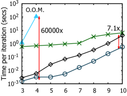
(a) Tensor order.

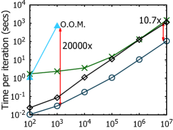
(b) Tensor dimensionality.

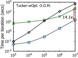
(c) Number of observable entries.

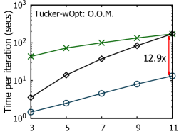
(d) Tensor rank.

Figure 6: The scalability of P-Tucker and competitors for large-scale synthetic tensors. O.O.M.: out of memory. P-Tucker exhibits 7.1-14.1x speed up compared to the state-of-the-art with respect to all aspects. Notice that Tucker-wOpt presents O.O.M. in most cases due to their limited scalability, and P-Tucker indicates the default memory-optimized version, not P-Tucker-Cache or P-Tucker-Approx.

IV-A3 Environment

P-Tucker is implemented in C with OpenMP and Armadillo libraries utilized for parallelization and linear algebra operations. From a practical viewpoint, P-Tucker does not automatically choose which optimizations to be used. Hence, users ought to select a method from P-Tucker and its variations in advance. For competitors, we use the original implementations provided by the authors ($\text{S-HOT}_{\text{scan}}$ , Tucker-CSF , and Tucker-wOpt ). We run experiments on a single machine with 20 cores/20 threads, equipped with an Intel Xeon E5-2630 v4 2.2GHz CPU and 512GB RAM. The default values for P-Tucker parameters $\lambda$ and $T$ are set to 0.01 and 20, respectively; for P-Tucker-Approx, the truncation rate per iteration is set to 0.2; for Tucker-CSF, we set the number of CSF allocations to 1 and choose a LAPACK SVD routine. We set the maximum running time per iteration to 2 hours and the maximum number of iterations to 20. In reporting running times, we use average elapsed time per iteration instead of total running time in order to confirm the theoretical complexities (see Table III), which are analyzed per iteration.

IV-B Data Scalability

We evaluate the data scalability of P-Tucker and other methods using both synthetic and real-world tensors.

IV-B1 Synthetic Data

We generate random tensors of size $I_{1}\!=\!I_{2}\!=\!...\!=\!I_{N}$ with real-valued entries between 0 and 1, varying the following aspects: tensor order, tensor dimensionality, the number of observable entries, and tensor rank. We assume that the core tensor $\boldsymbol{\mathscr{G}}$ is of size $J_{1}\!=\!J_{2}\!=\!...\!=\!J_{N}$.

Order. We increase the order $N$ of an input tensor from 3 to 10, while fixing $I_{n}\!=\!10^{2}$, $|\Omega|\!=\!10^{3}$, and $J_{n}\!=\!3$. As shown in Figure 6(a), P-Tucker exhibits the fastest running time with respect to the order. Although $\text{S-HOT}_{\text{scan}}$ and Tucker-CSF can decompose up to the highest-order tensor, they run 11$\times$ and 7.1$\times$ slower than P-Tucker, respectively. Tucker-wOpt runs 60000$\times$ (when $N=4$) slower than P-Tucker and shows O.O.M. (out of memory error) when $N\geq 5$. The enormous speed-gap between P-Tucker and Tucker-wOpt is explained by their time complexities. The speed of Tucker-wOpt mainly depends on the dimensionality term $I^{N}$, while P-Tucker relies on the rank term $J^{N}$ where $I>>J$.

Dimensionality. We increase the dimensionality $I_{n}$ of an input tensor from $10^{2}$ to $10^{7}$, while setting $N\!=\!3$, $|\Omega|\!=\!10\times I_{n}$, and $J_{n}\!=\!10$. As shown in Figure 6(b), P-Tucker consistently runs faster than other methods across all dimensionality. Tucker-wOpt runs $20000\times$ (when $I_{n}=10^{3}$) slower than P-Tucker and presents O.O.M. when $I_{n}\geq 10^{4}$. The speed-gap between P-Tucker and Tucker-wOpt is also described in a similar way to that of the order case. Though $\text{S-HOT}_{\text{scan}}$ and Tucker-CSF scale up to the largest tensor as well, they run 13.8$\times$ and 10.7$\times$ slower than P-Tucker, respectively.

Number of Observable Entries. We increase the number $|\Omega|$ of observable entries from $10^{3}$ to $10^{7}$, while fixing $N\!=\!3$, $I_{n}\!=\!10^{7}$, and $J_{n}\!=\!10$. As shown in Figure 6(c), P-Tucker, $\text{S-HOT}_{\text{scan}}$, and Tucker-CSF scale up to the largest tensor, while Tucker-wOpt shows O.O.M. for all tensors. P-Tucker presents the fastest factorization speed across all $|\Omega|$ and runs 14.1$\times$ and 44.3$\times$ faster than $\text{S-HOT}_{\text{scan}}$ and Tucker-CSF on the largest tensor with $|\Omega|=10^{7}$, respectively. Note that P-Tucker scales near linearly with respect to the number of observable entries.

Rank. We increase the rank $J_{n}$ from 3 to 11 with an increment of 2, while fixing $N\!=\!3$, $I_{n}\!=\!10^{6}$, and $|\Omega|\!=\!10^{7}$. As shown in Figure 6(d), P-Tucker, $\text{S-HOT}_{\text{scan}}$, and Tucker-CSF successfully factorize input tensors for all ranks. P-Tucker is the fastest in all cases; in particular, P-Tucker runs 12.9$\times$ and 13.0$\times$ faster than $\text{S-HOT}_{\text{scan}}$ and Tucker-CSF when $J_{n}=11$, respectively. Tucker-wOpt causes O.O.M. errors for all ranks.

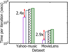
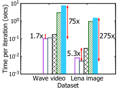
Figure 7: The scalability of P-Tucker and competitors on real-world tensors. P-Tucker and P-Tucker-Approx show the fastest running time across all datasets. An empty bar indicates that the corresponding method shows O.O.M. while factorizing the dataset.

IV-B2 Real-world Data

We measure the average running time per iteration of P-Tucker and other methods on the real-world datasets introduced in Section IV-A1. Due to the large scale of real-world tensors, Tucker-wOpt shows O.O.M. for two of them, which are set to blanks as shown in Figure 7. Notice that P-Tucker and P-Tucker-Approx succeed in decomposing the large-scale real-world tensors and run $1.7-275\times$ faster than competitors.

IV-C P-Tucker-Cache and P-Tucker-Approx

To investigate the effectiveness of P-Tucker-Cache, we vary the tensor order $N$ from $6$ to $10$, while fixing $I_{n}\!=\!10^{2}$, $|\Omega|\!=\!10^{3}$, and $J_{n}\!=\!3$. Figure 8 shows the running time and memory usage of P-Tucker and P-Tucker-Cache. P-Tucker uses $29.5\times$ less memory than P-Tucker-Cache for the largest order $N=10$. However, P-Tucker-Cache runs up to $1.7\times$ faster than P-Tucker, where the gap between the running times grows as tensor order $N$ grows since running times of P-Tucker-Cache and P-Tucker are mainly proportional to $N$ and $N^{2}$, respectively.

In the case of P-Tucker-Approx, we measure per-iteration time and full running time until convergence. Figures 9(a) and  9(b) illustrate the effectiveness of P-Tucker-Approx for the MovieLens dataset ($J_{n}\!=\!5$). P-Tucker-Approx gets faster than P-Tucker when iteration $\geq 3$ and converges $1.7\times$ earlier than P-Tucker. Moreover, the reconstruction error of P-Tucker-Approx is almost the same as that of P-Tucker. Note that one iteration corresponds to lines 3-6 in Algorithm 2.

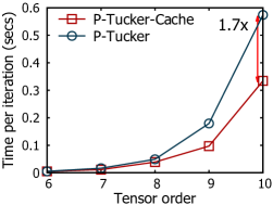
(a) Running time of P-Tucker
and P-Tucker-Cache.

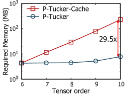
(b) Memory usage of P-Tucker
and P-Tucker-Cache.

Figure 8: Comparison results of P-Tucker and P-Tucker-Cache. P-Tucker-Cache runs up to 1.7$\times$ faster than P-Tucker for higher-order tensors, while P-Tucker decomposes the highest-order tensor with 29.5$\times$ less memory than P-Tucker-Cache.

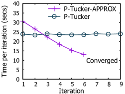
(a) Per-iteration running time of P-Tucker
and P-Tucker-Approx.

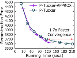
(b) Accuracy of P-Tucker and P-Tucker-Approx until convergence.

Figure 9: Comparison results of P-Tucker and P-Tucker-Approx. P-Tucker-Approx gets faster at every iteration and eventually runs quicker than P-Tucker (when iteration $\geq 3$). Furthermore, P-Tucker-Approx converges $1.7\times$ faster than P-Tucker with almost the same accuracy.

IV-D Effectiveness of Parallelization

We measure the speed-ups ($Time_{1}/Time_{T}$ where $Time_{T}$ is the running time using $T$ threads) and memory requirements of P-Tucker by increasing the number of threads from 1 to 20, while fixing $N\!=\!3$, $I_{n}\!=\!10^{6}$, and $|\Omega|\!=\!10^{7}$. Figure 10 shows near-linear speed up and memory requirements of P-Tucker regarding the number of threads. The linear speed-up implies that our parallelization works successfully, and the linearity of memory usage demonstrates that our theoretical memory complexity of P-Tucker matches the empirical result well. In addition, in order to verify the speed-up of dynamic scheduling, we compare P-Tucker with a naive parallelization which does not consider workload distributions. For the MovieLens dataset ($J_{n}=10$), the running time of P-Tucker (367.5s) is $1.5\times$ faster than that of the naive approach (552.7s), which demonstrates the effectiveness of dynamic scheduling.

Figure 10: The parallelization scalability of P-Tucker. Notice that the speed of P-Tucker increases linearly in terms of the number of threads, and the memory requirements of P-Tucker also scale near linearly with regard to the number of threads.

IV-E Real-World Accuracy

We evaluate the accuracy of P-Tucker and other methods on the real-world tensors. The evaluation metrics are reconstruction error and test root mean square error (RMSE); the former describes how precisely a method factorizes a given tensor, and the latter indicates how accurately a method estimates missing entries of a tensor, which is widely used by recommender systems. As shown in Figure 11, P-Tucker factorizes the tensors with 1.4-4.8$\times$ less reconstruction error and predicts missing entries of given tensors with 1.4-4.3$\times$ less test RMSE compared to the state-of-the-art. In particular, P-Tucker exhibits 1.4-2.6$\times$ higher accuracy than that of Tucker-wOpt, which also focuses on observed entries during factorizations. In Figure 11, we present $\text{S-HOT}_{\text{scan}}$ and Tucker-CSF with the same bar since they have similar accuracy, and the methods have low accuracies as they try to estimate missing entries as zeros. An omitted bar indicates that the corresponding method shows O.O.M. while decomposing the dataset.

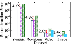
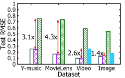
Figure 11: The accuracy of P-Tucker and competitors on the real-world tensors. P-Tucker achieves 1.4-4.8$\times$ higher accuracy compared to that of existing methods. An empty bar indicates that the corresponding method shows O.O.M. while factorizing the dataset.

V Discovery

We present discoveries on the latest MovieLens dataset introduced in Section IV-A. Existing methods cannot detect meaningful concepts or relations owing to their limited scalability or low accuracy. For instance, $\text{S-HOT}_{\text{scan}}$ and Tucker-CSF produce factor matrices mostly filled with zeros, which trigger highly inaccurate clustering. In contrast, P-Tucker successfully reveals the hidden concepts and relations such as a ‘Thriller’ concept, and a relation between a ‘Drama’ concept and hours (see Tables V and VI).

Concept Discovery. Our intuition for concept discovery is that each row of factor matrices represents latent features of the row. Thus, we can apply K-means clustering algorithm [31] on factor matrices to discover hidden concepts. In the case of movie-associated factor matrix, each row represents a latent feature of a movie. Therefore, by analyzing the clustered rows, P-Tucker excavates diverse movie genres, such as ‘Thriller’, ‘Comedy’, and ‘Drama’, and all the movies belonging to those genres are closely related (see Table V).

Relation Discovery. Core tensor $\boldsymbol{\mathscr{G}}$ plays an important role in discovering relations. An entry $(j_{1},...,j_{N})$ of $\boldsymbol{\mathscr{G}}$ is associated with the $j_{n}$th column of $\mathbf{A^{(n)}}$, and it implies that those columns are related to each other with a strength $\boldsymbol{\mathscr{G}}_{(j_{1},...,j_{N})}$. Hence, examining large values in $\boldsymbol{\mathscr{G}}$ gives us clues to find strong relations in a given tensor. For instance, P-Tucker succeeds in revealing relations between year and hour attributes such as $(2015,2pm)$ by investigating the $top-3$ largest value of a core tensor. In a similar way, P-Tucker finds strong relations between movie, year, and hour attributes, as summarized in Table VI.

VI Related Work

We review related works on CP and Tucker factorizations, and applications of Tucker decomposition.

CP Decomposition (CPD). Many algorithms have been developed for scalable CPD. GigaTensor [16] is the first distributed CP method running on the MapReduce framework. Park et al. [32] propose a distributed algorithm, DBTF, for fast and scalable Boolean CPD. In [33], Papalexakis et al. present a sampling-based, parallelizable method named ParCube for sparse CPD. AdaTM [34] is an adaptive tensor memoization algorithm for CPD of sparse tensors, which automatically tunes algorithm parameters. Kaya and Uçar [35] propose distributed memory CPD methods based on hypergraph partitioning of sparse tensors. Those algorithms are based on the ALS similarly to the conventional Tucker-ALS.

Since the above CP methods predict missing entries as zeros, tensor completion algorithms using CPD have gained increasing attention in recent years. Tomasi et al. [36] and Acar et al. [37] first address CPD models for tensor completion problems. Karlsson et al. [38] discuss parallel formulations of ALS and CCD++ for tensor completion in the CP format. Smith et al. [39] explore three optimization algorithms for high performance, parallel tensor completion: alternating least squares (ALS), stochastic gradient descent (SGD), and coordinate descent (CCD++). For distributed platforms, Shin et al. [24] propose CDTF and SALS, which are ALS-based CPD methods for partially observable tensors; Yang et al. [40] also offer SGD-based formulations for sparse tensors. Note that [24] and [39] offer a row-wise parallelization for CPD as P-Tucker does for Tucker decomposition.

TABLE V: Concept discoveries on the MovieLens dataset ($J=8,K=100$). Three notable movie concepts are found by P-Tucker.

Concept	Index	Attributes
	15535	Inception, 2010, $Action|Crime|Sci-Fi$
C1: Thriller	4880	Vanilla Sky, 2001, $Mystery|Romance$
	24694	The Imitation Game, 2014, $Drama|Thriller$
	6373	Bruce Almighty, 2003, $Drama|Fantasy$
C2: Comedy	16680	Home Alone 4, 2002, $Children|Comedy$
	12811	Mamma Mia!, 2008, $Musical|Romance$
	19822	Life of Pi, 2012, $Adventure|Drama|IMAX$
C3: Drama	11873	Once, 2006, $Drama|Musical|Romance$
	214	Before Sunrise, 1995, $Drama|Romance$

TABLE VI: Relation discoveries on the MovieLens dataset. Three notable relations between movie, year, and hour are found by P-Tucker.

Relations	$\boldsymbol{\mathscr{G}}$ Value	Details
R1:	$1.65\times 10^{6}$	Most preferred hours for drama genre
Drama-Hour		8 am, 4 pm, 1 am, 9 pm, and 6 pm
R2:	$1.29\times 10^{6}$	Comedy genre is favored in this period
Comedy-Year		(1997, 1998, 1999), (2005, 2006, 2007)
R3:	$2.29\times 10^{6}$	Most preferred hour for watching movies
Year-Hour		(2015, 2 pm), (2014, 0 am), (2013, 9 pm)

Tucker Factorization (TF). Several algorithms have been developed for TF. [12] presents an early work on TF, which is known as HOSVD. De Lathauwer et al. [13] propose Tucker-ALS, described in Algorithm 1. As the size of real-world tensors increases rapidly, there has been a growing need for scalable TF methods. One major challenge is the “intermediate data explosion” problem [16]. MET (Memory Efficient Tucker) [14] tackles this challenge by adaptively ordering computations and performing them in a piecemeal manner. HaTen2 [15] reduces intermediate data by reordering computations and exploiting the sparsity of real-world tensors in MapReduce. However, both MET and HaTen2 suffer from a limitation called M-bottleneck [17] that arises from explicit materialization of intermediate data. S-HOT [17] avoids M-bottleneck by employing on-the-fly computation. Kaya and Uçar [19] discuss a shared and distributed memory parallelization of an ALS-based TF for sparse tensors. [41] proposes optimizations of HOOI for dense tensors on distributed systems. The above methods depend on SVD for updating factor matrices, while P-Tucker utilizes a row-wise update rule.

There are also various accuracy-focused TF methods including Tucker-wOpt [18]. Yang et al. [42] propose another TF method that automatically finds a concise Tucker representation of a tensor via an iterative reweighted algorithm. Liu et al. [30] define the trace norm of a tensor, and present three convex optimization algorithms for low-rank tensor completion. Liu et al. [43] propose a core tensor Schatten 1-norm minimization method with a rank-increasing scheme for tensor factorization and completion. Note that these algorithms have limited scalability compared to P-Tucker since they are not fully optimized with respect to time and memory.

Applications of Tucker Factorization. Tucker factorization (TF) has been used for various applications. Sun et al. [3] apply a 3-way TF to a tensor consisting of (users, queries, Web pages) to personalize Web search. Bro et al. [44] use TF for speeding up CPD by compressing a tensor. Sun et al. [45] propose a framework for content-based network analysis and visualization which employs a biased sampling-based TF method. TF is also used for analyzing trends in the blogosphere [46].

VII Conclusion

We propose P-Tucker, a scalable Tucker factorization method for sparse tensors. By using ALS with a row-wise update rule, and with careful distributions of works for parallelization, P-Tucker successfully offers time and memory optimized algorithms with theoretical proof and analysis. P-Tucker runs 1.7-14.1$\times$ faster than the state-of-the-art with 1.4-4.8$\times$ less error, and exhibits near-linear scalability with respect to the number of observable entries and threads. We discover hidden concepts and relations on the latest MovieLens dataset with P-Tucker, which cannot be identified by existing methods due to their limited scalability or low accuracy. Future works include extending P-Tucker to distributed platforms such as Hadoop or Spark, and applying sampling techniques on observable entries to accelerate decompositions, while sacrificing little accuracy.

References

- [1] G. Dror, N. Koenigstein, Y. Koren, and M. Weimer, “The yahoo! music dataset and kdd-cup’11,” in KDD Cup, 2011, pp. 3–18.
- [2] D. M. Dunlavy, T. G. Kolda, and E. Acar, “Temporal link prediction using matrix and tensor factorizations,” TKDD, vol. 5, no. 2, pp. 10:1–10:27, 2011.
- [3] J.-T. Sun, H.-J. Zeng, H. Liu, Y. Lu, and Z. Chen, “Cubesvd: A novel approach to personalized web search,” in WWW, 2005, pp. 382–390.
- [4] J. Zhang, Y. Han, and J. Jiang, “Tucker decomposition-based tensor learning for human action recognition,” Multimedia Systems, vol. 22, no. 3, pp. 343–353, 2016.
- [5] X. Zhang, G. Wen, and W. Dai, “A tensor decomposition-based anomaly detection algorithm for hyperspectral image,” TGRS, vol. 54, no. 10, pp. 5801–5820, 2016.
- [6] N. Zheng, Q. Li, S. Liao, and L. Zhang, “Flickr group recommendation based on tensor decomposition,” in SIGIR, 2010, pp. 737–738.
- [7] E. E. Papalexakis, U. Kang, C. Faloutsos, N. D. Sidiropoulos, and A. Harpale, “Large scale tensor decompositions: Algorithmic developments and applications,” IEEE Data Eng. Bull., vol. 36, no. 3, pp. 59–66, 2013.
- [8] L. Sael, I. Jeon, and U. Kang, “Scalable tensor mining,” Big Data Research, vol. 2, no. 2, pp. 82 – 86, 2015, visions on Big Data.
- [9] N. Park, B. Jeon, J. Lee, and U. Kang, “Bigtensor: Mining billion-scale tensor made easy,” in CIKM, 2016.
- [10] B. Jeon, I. Jeon, L. Sael, and U. Kang, “Scout: Scalable coupled matrix-tensor factorization - algorithm and discoveries,” in ICDE, 2016.
- [11] T. G. Kolda and B. W. Bader, “Tensor decompositions and applications,” SIAM Review, vol. 51, no. 3, pp. 455–500, 2009.
- [12] L. R. Tucker, “Some mathematical notes on three-mode factor analysis,” Psychometrika, vol. 31, no. 3, pp. 279–311, 1966.
- [13] L. D. Lathauwer, B. D. Moor, and J. Vandewalle, “On the best rank-1 and rank-(R , R, … , R) approximation of higher-order tensors,” SIMAX, vol. 21, no. 4, pp. 1324–1342, 2000.
- [14] T. G. Kolda and J. Sun, “Scalable tensor decompositions for multi-aspect data mining,” in ICDM, 2008, pp. 363–372.
- [15] I. Jeon, E. E. Papalexakis, C. Faloutsos, L. Sael, and U. Kang, “Mining billion-scale tensors: algorithms and discoveries,” VLDB J., vol. 25, no. 4, pp. 519–544, 2016.
- [16] U. Kang, E. E. Papalexakis, A. Harpale, and C. Faloutsos, “Gigatensor: scaling tensor analysis up by 100 times - algorithms and discoveries,” in KDD, 2012, pp. 316–324.
- [17] J. Oh, K. Shin, E. E. Papalexakis, C. Faloutsos, and H. Yu, “S-hot: Scalable high-order tucker decomposition,” in WSDM, 2017.
- [18] M. Filipović and A. Jukić, “Tucker factorization with missing data with application to low-n-rank tensor completion,” Multidimensional systems and signal processing, vol. 26, no. 3, pp. 677–692, 2015.
- [19] O. Kaya and B. Uçar, “High performance parallel algorithms for the tucker decomposition of sparse tensors,” in ICPP, 2016, pp. 103–112.
- [20] S. Smith and G. Karypis, “Accelerating the tucker decomposition with compressed sparse tensors,” in Europar, 2017.
- [21] P.-L. Chen, C.-T. Tsai, Y.-N. Chen, K.-C. Chou, C.-L. Li, C.-H. Tsai, K.-W. Wu, Y.-C. Chou, C.-Y. Li, W.-S. Lin et al., “A linear ensemble of individual and blended models for music rating prediction,” KDDCup 2011, pp. 21–60, 2011.
- [22] Y. Koren, R. Bell, and C. Volinsky, “Matrix factorization techniques for recommender systems,” Computer, vol. 42, no. 8, pp. 30–37, 2009.
- [23] Y. Zhou, D. Wilkinson, R. Schreiber, and R. Pan, “Large-scale parallel collaborative filtering for the netflix prize,” in AAIM, 2008, pp. 337–348.
- [24] K. Shin, L. Sael, and U. Kang, “Fully scalable methods for distributed tensor factorization,” TKDE, vol. 29, no. 1, pp. 100–113, 2017.
- [25] L. N. Trefethen and D. Bau, Numerical Linear Algebra. SIAM, 1997.
- [26] T. G. Kolda, “Multilinear operators for higher-order decompositions,” Sandia National Laboratories, Tech. Rep., 2006.
- [27] P. C. Hansen, “The truncatedsvd as a method for regularization,” BIT Numerical Mathematics, vol. 27, no. 4, pp. 534–553, 1987.
- [28] OpenMP Architecture Review Board, “OpenMP application program interface version 4.0,” 2013.
- [29] S. Oh, N. Park, S. Lee, and U. Kang, “Supplementary material of p-tucker,” 2017. [Online]. Available: https://datalab.snu.ac.kr/ptucker/supple.pdf
- [30] J. Liu, P. Musialski, P. Wonka, and J. Ye, “Tensor completion for estimating missing values in visual data,” Pattern Anal. Mach. Intell., vol. 35, pp. 208–220, 2013.
- [31] T. Kanungo, D. M. Mount, N. S. Netanyahu, C. D. Piatko, R. Silverman, and A. Y. Wu, “An efficient k-means clustering algorithm: analysis and implementation,” TPAMI, vol. 24, no. 7, pp. 881–892, 2002.
- [32] N. Park, S. Oh, and U. Kang, “Fast and scalable distributed boolean tensor factorization,” in ICDE, 2017.
- [33] E. E. Papalexakis, C. Faloutsos, and N. D. Sidiropoulos, “Parcube: Sparse parallelizable tensor decompositions,” in ECML PKDD, 2012, pp. 521–536.
- [34] J. Li, J. Choi, I. Perros, J. Sun, and R. Vuduc, “Model-driven sparse cp decomposition for higher-order tensors,” in IPDPS, 2017, pp. 1048–1057.
- [35] O. Kaya and B. Uçar, “Scalable sparse tensor decompositions in distributed memory systems,” in SC, 2015, pp. 1–11.
- [36] G. Tomasi and R. Bro, “Parafac and missing values,” Chemometr. Intell. Lab. Syst., vol. 75, no. 2, pp. 163–180, 2005.
- [37] “Scalable tensor factorizations for incomplete data,” Chemometrics and Intelligent Laboratory Systems, vol. 106, pp. 41 – 56, 2011.
- [38] L. Karlsson, D. Kressner, and A. Uschmajew, “Parallel algorithms for tensor completion in the cp format,” Parallel Computing, vol. 57, pp. 222 – 234, 2016.
- [39] S. Smith, J. Park, and G. Karypis, “An exploration of optimization algorithms for high performance tensor completion,” SC, 2016.
- [40] F. Yang, F. Shang, Y. Huang, J. Cheng, J. Li, Y. Zhao, and R. Zhao, “Lftf: A framework for efficient tensor analytics at scale,” Proc. VLDB Endow., vol. 10, no. 7, pp. 745–756, Mar. 2017.
- [41] V. T. Chakaravarthy, J. W. Choi, D. J. Joseph, X. Liu, P. Murali, Y. Sabharwal, and D. Sreedhar, “On optimizing distributed tucker decomposition for dense tensors,” CoRR, vol. abs/1707.05594, 2017.
- [42] L. Yang, J. Fang, H. Li, and B. Zeng, “An iterative reweighted method for tucker decomposition of incomplete tensors,” IEEE Trans. Signal Processing, vol. 64, no. 18, pp. 4817–4829, 2016.
- [43] Y. Liu, F. Shang, W. Fan, J. Cheng, and H. Cheng, “Generalized higher-order orthogonal iteration for tensor decomposition and completion,” in NIPS, 2014, pp. 1763–1771.
- [44] R. Bro, N. Sidiropoulos, and G. Giannakis, “A fast least squares algorithm for separating trilinear mixtures,” in Int. Workshop Independent Component and Blind Signal Separation Anal, 1999, pp. 11–15.
- [45] J. Sun, S. Papadimitriou, C.-Y. Lin, N. Cao, S. Liu, and W. Qian, “Multivis: Content-based social network exploration through multi-way visual analysis,” in SDM, 2009, pp. 1064–1075.
- [46] Y. Chi, B. L. Tseng, and J. Tatemura, “Eigen-trend: trend analysis in the blogosphere based on singular value decompositions,” in CIKM, 2006.