Helioseismic and Neutrino Data Driven Reconstruction of Solar Properties

Abstract

In this work we use Bayesian inference to quantitatively reconstruct the solar properties most relevant to the solar composition problem using as inputs the information provided by helioseismic and solar neutrino data. In particular, we use a Gaussian process to model the functional shape of the opacity uncertainty to gain flexibility and become as free as possible from prejudice in this regard. With these tools we first readdress the statistical significance of the solar composition problem. Furthermore, starting from a composition unbiased set of standard solar models we are able to statistically select those with solar chemical composition and other solar inputs which better describe the helioseismic and neutrino observations. In particular, we are able to reconstruct the solar opacity profile in a data driven fashion, independently of any reference opacity tables, obtaining a 4% uncertainty at the base of the convective envelope and 0.8% at the solar core. When systematic uncertainties are included, results are 7.5% and 2% respectively. In addition we find that the values of most of the other inputs of the standard solar models required to better describe the helioseismic and neutrino data are in good agreement with those adopted as the standard priors, with the exception of the astrophysical factor $S_{11}$ and the microscopic diffusion rates, for which data suggests a 1% and 30% reduction respectively. As an output of the study we derive the corresponding data driven predictions for the solar neutrino fluxes.

1 Introduction

Standard Solar Models (SSMs; Bahcall & Ulrich, 1988; Turck-Chieze et al., 1988; Bahcall & Pinsonneault, 1992, 1995; Bahcall et al., 2001, 2005b; Peña-Garay & Serenelli, 2008; Serenelli et al., 2011; Vinyoles et al., 2017) describe the Sun present day properties as a result of its evolution starting at the pre-main sequence. A set of observational parameters are taken as constraints that SSMs calculations have to satisfy by construction. They include the present surface abundances of heavy elements and surface luminosity of the Sun, as well as its age, radius and mass. The modeling relies on some simplifying assumptions such as hydrostatic equilibrium, spherical symmetry, homogeneous initial composition, and evolution at constant mass. SSMs have been constantly refined by including updated experimental results and observations regarding the values in physical input parameters. Examples include the values of the nuclear reaction rates and the surface abundances. There have also been improvements on the accuracy of the calculation of the constituent quantities like the equation of state and the radiative opacity, as well as the inclusion of new physical effects like the diffusion of elements.

The Sun burns, i.e. it generates power through nuclear fusion, with the basic energy source being the burning of four protons into an alpha particle, two positrons, and two neutrinos. Being only weakly interacting, the neutrinos can exit the Sun relatively unaffected. Thus they give us the opportunity to learn about the solar interior and test in an almost direct way our understanding of nuclear energy production in the solar core (Bahcall, 1964). With this objective the original neutrino experiments were designed, their goal being somewhat diverted by the appearance of the then called “solar neutrino problem” (Bahcall et al., 1968; Bahcall & Davis, 1976). Thanks to the increasing experimental accuracy of the measured neutrino flux in radiochemical experiments Chlorine (Cleveland et al., 1998), Gallex/GNO (Kaether et al., 2010) and SAGE (Abdurashitov et al., 2009), together with the upcoming of the real-time experiments, Super-Kamiokande (Hosaka et al., 2006; Cravens et al., 2008; Abe et al., 2011; Koshio, 2015), SNO (Aharmim et al., 2013) and Borexino (Bellini et al., 2011, 2014b, 2010, 2014a), we have now reached the solution of the problem. It implied the modification of the Standard Model (of particle physics) with the addition of neutrino masses and leptonic mixing which imply both flavour transition of the solar neutrinos from production to detection (Pontecorvo, 1968; Gribov & Pontecorvo, 1969), and non-trivial effects in their flavour evolution when crossing dense regions of matter, the so called LMA-MSW flavour transitions (Wolfenstein, 1978; Mikheev & Smirnov, 1985).

Moreover the Sun beats. In first approximation it can be considered to be a non-radial oscillator and the study of its frequency pattern offers powerful insights as well (for example, see Basu & Antia 2008). In particular, the sound speed as a function of depth can be reconstructed to precision of order 0.1%. The transition from radiative to convective energy transport, or abrupt changes in the solar thermal structure from ionization, induce acoustic glitches that can be precisely localized; thus with that level of precision it is possible to infer the depth of the convective envelope with 0.2% accuracy and the surface helium abundance with 1.5% accuracy. This is, the solar structure is well constrained and the Sun can be used as a solid benchmark for stellar evolution and as a laboratory for fundamental physics (see e.g. Fiorentini et al., 2001; Ricci & Villante, 2002; Bottino et al., 2002; Gondolo & Raffelt, 2009; Vinyoles et al., 2015; Vinyoles & Vogel, 2016).

As usual in the history of physics, better experimental information opens new questions. So in parallel to the increased precision on both solar neutrino detection and helioseismic solar results, a new puzzle emerged in the consistency of SSMs (Bahcall et al., 2005a). SSMs built in the last decade of the last century had notable successes in predicting the helioseismology related measurements (Bahcall & Pinsonneault, 1992, 1995; Christensen-Dalsgaard et al., 1996; Bahcall et al., 2001, 2005b). A key element to this agreement was the input value of the abundances of heavy elements on the surface of the Sun used to compute SSMs (Grevesse & Sauval, 1998). But in the second half of the first decade of the 21st century new determinations of these abundances became available and they pointed towards substantially lower values (Asplund et al., 2006, 2009). The SSMs built incorporating such lower metallicities failed at explaining the helioseismic observations (Bahcall et al., 2005a).

So far there has not been a successful solution of this puzzle as no obvious changes in the Sun modeling have been found which could be able to account for this discrepancy  (Castro et al., 2007; Guzik & Mussack, 2010; Serenelli et al., 2011). This has led to the construction of two different sets of SSMs, one based on the older solar abundances (Grevesse & Sauval, 1998) implying high metallicity, and one assuming lower metallicity as inferred from the “newer” determinations of the solar abundances (Asplund et al., 2006, 2009). In a subsequent set of works (Serenelli et al., 2009; Serenelli et al., 2011; Vinyoles et al., 2017) the neutrino fluxes and helioseismic predictions corresponding to such two models were detailed, based on updated versions of the solar model calculations.

Alternatively, attempts to use the information from helioseismic and neutrino observations to better determine the solar chemical composition and other solar properties started to be put forward (Delahaye & Pinsonneault, 2006; Villante et al., 2014). The technical complication arises from the fact that both neutrino and helioseismic results are outputs of the standard solar model simulations while chemical composition and the other properties to be inferred are inputs. We are faced then with a common issue in multivariable analysis, the consistent estimation of the values of input parameters (some even with unknown functional dependence) which can provide a valid set of outputs within a given statistical level of agreement with some data. Before the advent of fast computing facilities this could only be attempted by partially reducing the number of inputs to be allowed to vary. For example, in Villante et al. (2014) the problem was analyzed in terms of three continuous multiplicative factors (the abundance of volatiles, that of refractories and that of Ne) to parametrize the allowed departures of the standard solar model inputs from the adopted priors of the two model versions. Furthermore, for the opacity profile – an input which is not a parameter but a function – assumptions about its functional form and allowed range of functional variation had to be assumed.

In this work we take a step forward in this program by making use of Bayesian inference methods applied with specific numerical tools such as MultiNest (Feroz & Hobson, 2008; Feroz et al., 2009; Feroz et al., 2013) which have been developed precisely to make such inference in large parameter spaces which may contain multiple modes and pronounced degeneracies. Furthermore we introduce the use of Gaussian process (GP), a non-parametric regression method, to reconstruct the opacity profile and its uncertainty without assuming a specific functional form.

The outline of the paper is as follows. In Sec. 2 we present a brief introduction to the Bayesian parameter inference methods which we are using in this work. Section 3 discusses the issues arising in the parametrization of the opacity profile function for which we first describe the traditional linear form in Sec. 3.1. Section 3.2 presents the alternative non-parametric GP method to reconstruct the opacity profile (see also appendix B where we introduce the main concepts in GP method for non-parametric functional reconstruction). In Section 4 we first apply this methodology to readdress the solar composition problem by evaluating a test of significance of the two B16 SSMs (Vinyoles et al., 2017) and using the two prescriptions of the profiles of the opacity and its uncertainty (linear and GP). We find, as expected, that allowing for the most flexible GP form of the opacity uncertainty profile decreases the evidence against the B16-AGSS09met model but it is still strongly disfavoured. Section 5 contains our evaluation of the optimum solar composition, opacity profile and other solar parameters, to describe the helioseismic and neutrino data by Bayesian inference starting with a composition unbiased set of standard solar models. As an output of the study we derive the corresponding prediction for the solar neutrino fluxes. Finally in section 6 we summarize our conclusions. Details of the construction of the Likelihood function used in the analysis of the helioseismic and neutrino data are summarized in the Appendix A.

2 Statistical Framework

Bayesian inference methods provide a consistent approach to the estimation of a set of parameters $\boldsymbol{\Theta}$ in a model $M$ for the data $\boldsymbol{D}$. Bayes’ theorem states that under the assumption that a model $M$ is true, complete inference of its parameters is given by the posterior distribution,

$$\Pr(\boldsymbol{\Theta}|\boldsymbol{D},M)=\frac{\Pr(\boldsymbol{D}|\boldsymbol{\Theta},M)\Pr(\boldsymbol{\Theta}|M)}{\Pr(\boldsymbol{D}|M)}=\frac{\mathcal{L}(\boldsymbol{\Theta})\pi(\boldsymbol{\Theta})}{\mathcal{Z}},$$ (1)

where $\mathcal{L}(\boldsymbol{\Theta})\equiv\Pr(\boldsymbol{D}|\boldsymbol{\Theta},M)$ is the likelihood function. The prior probability density of the parameters is given by $\pi(\boldsymbol{\Theta})\equiv\Pr(\boldsymbol{\Theta}|M)$, and should always be normalized, i.e., it should integrate to unity. Conversely the evidence, $\mathcal{Z}_{i}=\Pr(\boldsymbol{D}|M_{i})$, is the likelihood for the model quantifying how well the model describes the data.

From the posterior distribution one can construct reparametrization invariant Bayesian credible intervals by defining the “credible level” of a value $\eta=\eta_{0}$ of a subset of parameters simply as the posterior volume within the likelihood of that value,

$${\rm CL}(\eta_{0})=\int_{\mathcal{L}(\eta)>\mathcal{L}(\eta_{0})}\Pr(\eta|\boldsymbol{D}){\rm d}\eta.$$ (2)

This function can be converted to the “number of $\sigma$’s” in the usual manner as

$$S=\sqrt{2}{\rm erfc}^{-1}(1-{\rm CL}).$$ (3)

Bayesian statistics is mostly suited to make a relative statement about the plausibility of a given model $M_{i}$ versus another $M_{j}$ by comparing their respective posterior probabilities. This is quantified by means of the Bayes factor

$$\mathcal{B}_{ij}=\frac{\mathcal{Z}_{i}}{\mathcal{Z}_{j}}$$ (4)

which is the ratio of the evidences. Jeffrey’s scale is often used for the interpretation of the Bayes factors (see Table 1).

$\left|\ln(\mathcal{B}_{ij})\right|$	Strength of Evidence
$<1.0$	Inclusive
1.0–2.5	Weak to Moderate
2.5–5	Moderate to Strong
$>5.0$	Strong to Very Strong/Decisive

Table 1: Jeffrey’s scale for interpretation of the Bayes factors

This gives what the ratio of posterior probabilities for the models would be if the overall prior probabilities for the two models were equal. Or in other words it shows by how much the probability ratio of model $M_{i}$ to model $M_{j}$ changes in the light of the data, and thus can be viewed as a numerical measure of evidence supplied by the data in favour of one hypothesis over the other.

It is also possible to make an absolute test of significance of a given model $M$ by using the prior predictive distribution, which is to be understood as a distribution of the possible observable outputs $\vec{\cal O}$,

$$\Pr(\vec{\cal O})=\int\Pr(\vec{\cal O}|\boldsymbol{\Theta})\pi(\boldsymbol{\Theta}){\rm d}^{N}\boldsymbol{\Theta}$$ (5)

to determine the probability distribution function for some statistics $\mathcal{T}(\vec{\cal O})$ and compare it with what was actually observed. This would be done as usual by calculating the p-value

$$p=\Pr(\mathcal{T}(\vec{\cal O})\geq\mathcal{T}(\vec{\cal O}^{\rm dat}))$$ (6)

In this work we use MultiNest (Feroz & Hobson, 2008; Feroz et al., 2009; Feroz et al., 2013), a Bayesian inference tool which, given the prior and the likelihood, calculates the evidence with an uncertainty estimate, and generates posterior samples from distributions that may contain multiple modes and pronounced (curving) degeneracies in high dimensions.

The general procedure which we will follow is to use MC generated sets of SSMs obtained for different choices of the model input parameters. These are 20 quantities: the Sun luminosity – $L_{\odot}$– , the Sun diffusion, the Sun age – $t_{\odot}$– , 8 Nuclear Rates – $S_{11}$, $S_{33}$, $S_{34}$, $S_{17}$, $S_{e7}$, $S_{114}$, $S_{\rm hep}$, $S_{116}$ –, and 9 Element Abundances – C, N, O, Ne, Mg, Si, S, Ar, Fe –. Finally, one must also input some parametrization of the Opacity profile and its uncertainty (more below).

The sets of models are generated according to priors for these inputs which reflect our knowledge of those (knowledge which is independent of the data used in our analysis). Generically the priors are assumed to be Gaussian distributed. The numerical values for the mean and standard distributions for the first 20 inputs are given in Vinyoles et al. (2017). The assumed priors for the first 11 inputs are common to all models generated, while for the abundances there are two different sets of priors corresponding to high-Z and low-Z compositions leading to the B16-GS98 and B16-AGSS09met model subsets respectively.

Following the procedure outlined above we confront these models with the data from helioseismology and neutrino oscillation experiments described in the Appendix A. They amount to an effective number of 32 data points from helioseismic data plus a large number of points from the global analysis of neutrino oscillation data used in Bergström et al. (2016) with which we build the likelihood function

$$-2\ln\mathcal{L}(\boldsymbol{\Theta})=\sum_{i,j}\frac{({\cal O}^{\rm mod}_{i}(\boldsymbol{\Theta})-{\cal O}^{\rm dat}_{i})}{\sigma^{\rm dat}_{i}}(\rho^{\rm dat})^{-1}_{ij}\frac{({\cal O}^{\rm mod}_{j}(\boldsymbol{\Theta})-{\cal O}^{\rm dat}_{j})}{\sigma^{\rm dat}_{j}}$$ (7)

where ${\cal O}^{\rm mod}_{i}(\boldsymbol{\Theta})$ are the model predicted values for all these observables obtained by MC generation for a given set of values of the model inputs $\boldsymbol{\Theta}$. The correlation matrix $\rho^{\rm dat}_{ij}=\delta_{ij}$ for $i,j=1,32$ but it is not diagonal for all the other entries which correspond to the neutrino oscillation data. Effectively the neutrino oscillation part of the likelihood can be approximated by 8 data points corresponding to the extracted solar flux normalizations given in the last column in table 6 and with the correlation matrix in Eq. (23).

With these likelihood functions we can obtain the posterior distribution for some (or all) of the input parameters. These posterior distributions will quantify how the inclusion of this additional data affects our knowledge of those properties of the Sun.

Also, as described above, we can use the prior predictive distribution corresponding to the two variants of the SSM’s to carry out a test of significance and to obtain their corresponding p-values. For this, we define the statistical test $\mathcal{T}(\vec{\cal O})$ (where $\vec{\cal O}$ is an n-dimensional vector containing possible values for the n observables):

$$\mathcal{T}(\vec{\cal O})=(\vec{\cal O}-\vec{\langle}\vec{\cal O}^{\rm mod}\rangle)^{T}(C_{\rm dat}+C_{\rm mod})^{-1}(\vec{\cal O}-\vec{\langle}\vec{\cal O}^{\rm mod}\rangle)$$ (8)

where $C_{{\rm dat},ij}=\rho^{\rm dat}_{ij}\sigma^{\rm dat}_{i}\sigma^{\rm dat}_{j}$ is the covariance matrix associated to the experimental uncertainties, and

$$C_{{\rm mod},ij} = \langle({\cal O}^{\rm mod}_{i}-\bar{\cal O}^{\rm mod}_{i})({\cal O}^{\rm mod}_{j}-\bar{\cal O}^{\rm mod}_{j})\rangle$$ (9)

$$\equiv \langle({\cal O}^{\rm mod}_{i}-\bar{\cal O}^{\rm mod}_{i})\rangle\rho_{{\rm mod},ij}\langle({\cal O}^{\rm mod}_{i}-\bar{\cal O}^{\rm mod}_{i})\rangle$$

is the model covariance matrix obtained from the MC generated model predictions by sampling over the model input priors about their means $\bar{\cal O}^{\rm mod}_{i}\equiv\langle{\cal O}^{\rm mod}_{i}\rangle$.

The probability distribution of $\mathcal{T}(\vec{\cal O})$ can be determined from the MC model predictions by generating pseudo experimental results $\vec{\cal O}$ normally distributed according to $C_{\rm dat}$ around each $\vec{\cal O}^{\rm mod}$ in the MC generated model samples, and computing for each pseudo experimental result the corresponding value of $\mathcal{T}$. We find that, as expected, the probability distribution of $\mathcal{T}(\vec{\cal O})$ follows very closely a $\chi^{2}_{n}$-distribution.

Unlike the first twenty inputs listed above, the opacity profile is not a numerical parameter but a function. We describe next two different procedures to parametrize the uncertainty in its prior.

3 Treatment of the radiative opacity

A fundamentally important physical ingredient in solar models that cannot be quantified by just one parameter is the radiative opacity, which is a complicated function of temperature ($T$), density ($\rho$) and chemical composition of the solar plasma expressed here in terms of the helium ($Y$) and heavy elements mass fractions ($Z_{i}$, where $i$ runs over all metals included in opacity calculations). In our calculations, we take as a reference the atomic opacities from OP (Badnell et al., 2005) complemented at low temperatures by molecular opacities from Ferguson et al. (2005). The magnitude and functional form of its uncertainty is currently not well constrained in available opacity calculations. As a result, representation of the uncertainty in radiative opacity by a single parameter (Serenelli et al., 2013) or by taking the difference between two alternative sets of opacity calculations (Bahcall et al., 2006; Villante et al., 2014) are strong simplifications, at best. In this paper, instead, we choose to follow a general and flexible approach based on opacity kernels originally developed by Tripathy & Christensen-Dalsgaard (1998) and later on by Villante (2010), which we describe next.

The reference opacity calculation $\bar{\kappa}(\rho,T,Y,Z_{i})$ can be modified by a generic function of T, $\rho$, $Y$ and $Z_{i}$. For simplicity, we assume that opacity variations are parametrized as a function of $T$ alone such that

$$\kappa(\rho,\,T,\,Y,\,Z_{\rm i})=\left[1+\delta\kappa_{\rm I}(T)\right]\,\overline{\kappa}(\rho,\,T,\,Y,\,Z_{\rm i})$$ (10)

where $\delta\kappa_{\rm I}(T)$ is an arbitrary function that we call intrinsic opacity change. The Sun responds linearly even to relatively large opacity variations $\delta\kappa_{\rm I}(T)$ Tripathy & Christensen-Dalsgaard (1998); Villante (2010). Thus, the fractional variation of a generic SSM prediction

$$\delta Q\equiv Q/\bar{Q}-1,$$ (11)

where $Q$ ($\bar{Q}$) corresponds to the modified (reference) value, can be described as

$$\delta Q=\int\frac{dT}{T}K_{Q}(T)\delta\kappa_{\rm I}(T)$$ (12)

by introducing a suitable kernel $K_{Q}(T)$ that describes the response of $Q$ to changes in the opacity at a given temperature. We determine the kernels $K_{Q}(T)$ numerically by studying the response of solar models to localized opacity changes as it was done in Tripathy & Christensen-Dalsgaard (1998). Our results agree very well in all cases except for variations in the chemical composition because our models include gravitational settling.

The evaluation of $\delta Q$ is subject to the choice we make for $\delta\kappa_{\rm I}(T)$. In Haxton & Serenelli (2008) and Serenelli et al. (2013) the opacity error was modeled as a 2.5% constant factor at $1\sigma$ level, comparable to the maximum difference between the OP and OPAL (Iglesias & Rogers, 1996) opacities in the solar radiative region. Villante (2010) showed that this prescription underestimates the contribution of opacity uncertainty to the sound speed and convective radius error budgets because the opacity kernels for these quantities are not positive definite and integrate to zero for $\delta\kappa(T)={\rm const}$. Later on, Villante et al. (2014) considered the temperature-dependent difference between OP and OPAL opacities as $1\sigma$ opacity uncertainty. However, it is by no means clear that this difference is a sensible measure of the actual level of uncertainty in current opacity calculations.

Based on the previous reasons, here we follow a different approach inspired by the most recent experimental and theoretical results and some simple assumptions. The contribution of metals to the radiative opacity is larger at the bottom of the convective envelope ($\sim 70\%$) than at the solar core ($\sim 30\%$). Moreover, at the base of the convective envelope, relevant metals like iron are predominantly in an L-shell configuration, for which atomic models are more uncertain than for the K-shell configuration that predominates at solar core conditions. Also, in a recent theoretical analysis of line broadening modeling in opacity calculations, Krief et al. (2016) have found that uncertainties linked to it are larger at the base of the convective envelope than in the core. These arguments suggest that opacity calculations are more accurate at the solar core than in the region around the base of the convective envelope. It is thus natural to consider error parameterizations that allow opacity to fluctuate by a larger amount in the external radiative region than in the center of the Sun.

3.1 Linear Parametrization of Intrinsic Opacity Profile Uncertainty

Taking all this into account, we consider the following parameterization for the intrinsic opacity change (relative to some reference value):

$$\delta\kappa_{I}(T)=a+b\;\frac{\log_{10}(T_{\rm C}/T)}{\tau}$$ (13)

where $\tau=\log_{10}(T_{\rm C}/T_{\rm CZ})=0.9$, $T_{\rm C}$ and $T_{\rm CZ}$ are the temperatures at the solar center and at the bottom of the convective zone respectively. This equation is applied only up to the lower regions of the convective envelope, where convection is adiabatic and changes in the opacity do not modify the solar structure. Opacity changes in the uppermost part of the convective envelope and atmosphere are absorbed in the solar calibration by changes in the mixing length parameter and, in sound speed inversions, by the surface term. In the context of SSMs, they will not produce changes in the solar properties considered in the present work.

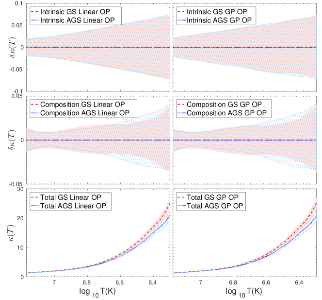
Technically, the opacity uncertainty is incorporated in our model generation by extending the parameter space with 2 more independent inputs, $a$ and $b$, each with a gaussian prior with zero mean and variances $\sigma_{a}$ and $\sigma_{b}$, respectively. This corresponds to assuming that the opacity error at the solar center is $\sigma_{\rm min}=\sigma_{a}$, while it is given by $\sigma_{\rm out}\simeq\sqrt{\sigma^{2}_{a}+\sigma^{2}_{b}}$ at the base of the convective zone. We fix $\sigma_{\rm in}=\sigma_{a}=2\%$ which is the average difference of the OP and OPAL opacity tables. This is also comparable to differences found with respect to the new OPAS opacity tables (Mondet et al., 2015) for the AGSS09 solar composition, the only one available in OPAS. The more recent OPLIB tables from Los Alamos (Colgan et al., 2016) show much larger differences in the solar core, about 10 to 12% lower than OP and up to 15% lower than OPAS. However, OPLIB opacities lead to solar models that predict too low $Y_{S}$ and $\Phi({\rm{}^{7}Be})$ and $\Phi({\rm{}^{8}B})$ fluxes that cannot be reconciled with data. For $\sigma_{\rm out}$ we choose 7% (i.e. $\sigma_{b}=6.7\%$), motivated by the recent experimental results of Bailey et al. (2015) that have measured the iron opacity at conditions similar to those at the base of the solar convective envelope and have found a $7\%\pm 4\%$ increase with respect to the theoretical expectations. The resulting prior for the intrinsic opacity profile uncertainty is shown in the upper left panel in Fig. 1 for both B16 models. Given the generated values for those two parameters we construct the function $\delta\kappa_{I}(T)$ as in Eq. (13) and with that we compute the corresponding change in the output quantities as in Eq. (12).

As we will see below and was also discussed by Vinyoles et al. (2017), it turns out that our ad-hoc linear parametrization of the intrinsic opacity uncertainty is not flexible enough to accommodate the tension between B16-AGSS09met model and data (especially sound speed data). This parametrization was chosen for its simplicity, whereas in fact the shape of the opacity uncertainty function is unknown. Thus, in the next section we turn to a more general modeling of the intrinsic opacity uncertainty based on a Gaussian Process approach. A brief introduction of the general method is given in Appendix B.

Figure 1: Priors for the intrinsic opacity change (upper panels), the composition opacity change, Eq. (20) (central panels), and the total opacity profile (lower panels). Left correspond to the linear parametrization of the intrinsic opacity uncertainty while right corresponds to the Gaussian Process one.

3.2 Gaussian Process Reconstruction of the Opacity Profile

Our goal is to define the uncertainty of the opacity profile without using parameterized functions and to reconstruct the intrinsic opacity change $\delta\kappa_{\rm I}(T)$ that can lead to a better agreement with the data. In order to do this, following the discussion in Sec. 3.1, we assume that $\delta\kappa_{\rm I}(T)$ is a gaussian variable with mean is $\mu_{P}(T)\equiv 0$ with a temperature dependent variance $\sigma(T)$ which allows for 2% uncertainty in the solar center and 7% at the base of the convective zone, i.e.:

$$\sigma(T)=0.02+(0.07-0.02)\cdot\frac{\log_{10}(T_{\rm C}/T)}{\tau}\;.$$ (14)

As the values of the opacity at two different temperatures $T$ and $T^{\prime}$ may be not independent, we introduce a prior covariance function $C_{P}(T,T^{\prime})$. A possible choice is

$$C_{P}(T,T^{\prime})=\sigma(T)\sigma(T^{\prime})\rho(T,T^{\prime}),$$ (15)

with

$$\rho(T,T^{\prime})=\mathrm{exp}\left[-\frac{1}{2}\left(\frac{\log_{10}T-\log_{10}T^{\prime}}{\tau\,L}\right)^{2}\right].$$ (16)

Here $L$ determines the characteristic correlation length over which $\delta\kappa_{\rm I}(T)$ can vary significantly and it is the only hyperparameter in our analysis. According to the above definition, $L=1$ means maximum correlation between the opacity at the edge of the convective zone and at the center. If $L$ is too large the correlation is too strong and the model is over constrained. If, on the other hand, $L$ is too small, we are allowing opacity errors to dominate the output of solar models, and we can barely learn anything from the data. Moreover, there is a physically motivated lower bound for $L$ given by the temperature range over which the opacity can vary substantially. In the solar interior $|\partial\ln{\kappa}/\partial\ln{T}|<2$ (Colgan et al., 2016). From this, the smallest temperature range over which $\Delta\ln{\kappa}\approx 1$ is $\Delta\ln{T}\approx 0.5$, i.e. $L_{\rm min}\approx 0.2$.

To implement the Gaussian Process intrinsic opacity uncertainty in our analysis we start by choosing a set of $N$ points in which we evaluate the function $\delta\kappa_{{\rm I}i}=\delta\kappa_{\rm I}(T_{i})$. We take $N=11$ and choose the points to be uniformly distributed in $\log_{10}T$ between 6.3 and 7.2. The parameter space for model generation is thus extended with 12 more input parameters: the length $L$ and the 11 $\delta\kappa_{{\rm I}i}$ values. For the correlation length we assume a uniform prior in $\log_{10}L$ between $\log_{10}0.2$ and $\log_{10}1$. The values $\delta\kappa_{{\rm I}i}$ are generated according to prior distribution defined by Eqs. (14-16), together with $\mu_{P}(T)\equiv 0$. Given a set of values for the 11 $\delta\kappa_{Ii}$’s we construct the full function $\delta\kappa_{I}(T)$ by linear interpolation between these values and with that we compute the corresponding change in the output predictions as in Eq. (12). The resulting prior distribution of the intrinsic opacity change is shown in the upper right panel of Fig. 1. As seen in the figure, the ranges of uncertainty profiles for the linear parametrization and the GP opacity are very similar. They do, however, lead to different conclusions when testing the SSM’s models versus the data (in particular vs helioseismic data) as described in Sec. 4.

3.3 The Degeneracy between Opacity and Composition Effects

The properties of the Sun depend on its opacity profile $\kappa_{\rm SSM}(T)$ that we define as:

$$\kappa_{\rm SSM}(T)=\kappa(\rho(T),\,T,\,Y(T),\,Z_{i}(T))$$ (17)

where $\rho(T)$, $Y(T)$ and $Z_{i}(T)$ describe the density, helium and heavy element abundances stratifications as a function of the temperature of the solar plasma in a given SSM. This is indeed the quantity that determines the efficiency of radiative energy transport and, thus, the temperature gradient at each point of the Sun and that is plotted in the lower panels of Fig. 1 for both B16 models. When considering an intrinsic opacity change $\delta\kappa_{\rm I}(T)$ and/or other input parameters in the SSMs are varied, the SSM needs to be recalibrated, thus obtaining different density and chemical abundances stratifications with respect to the reference SSM. As a consequence, the total variation of the solar opacity profile is given by:

$$\delta\kappa_{\rm SSM}(T) \equiv \kappa_{\rm SSM}(T)/\overline{\kappa}_{\rm SSM}(T)-1\simeq$$ (18)

$$\simeq \delta\kappa_{\rm I}(T)+\frac{\partial\ln\kappa}{\partial\ln\rho}\delta\rho(T)+\frac{\partial\ln\kappa}{\partial\ln Y}\delta Y(T)+$$

$$+\sum_{i}\frac{\partial\ln\kappa}{\partial\ln Z_{i}}\delta Z_{i}(T)$$

where $\delta\rho(T)$, $\delta Y(T)$ and $\delta Z_{i}(T)$ are the fractional variations of density and elemental abundances in the perturbed Sun with respect to the reference SSM, evaluated at a fixed temperature $T$.

As discussed above, the metal abundances $Z_{i}(T)$ are derived quantities that have to be obtained as a results of numerical solar modeling. However, when we consider a modification of the surface composition $\{z_{i}\}$, expressed here in terms of the quantities $z_{i}\equiv Z_{i,\rm S}/X_{\rm S}$ where $Z_{i,\rm S}$ is the surface abundance of the $i-$element and $X_{\rm S}$ is that of hydrogen, we can approximately assume $\delta Z_{i}(T)\simeq\delta z_{i}$ where $\delta z_{i}$ is the fractional variation of $z_{i}$ with respect to some reference value. As a consequence, Eq. (18) can be rewritten as:

$$\delta\kappa_{\rm SSM}(T)=\delta\kappa_{\rm I}(T)+\delta\kappa_{\rm Z}(T)+\frac{\partial\ln\kappa}{\partial\ln\rho}\delta\rho(T)+\frac{\partial\ln\kappa}{\partial\ln Y}\delta Y(T)$$ (19)

where the composition opacity change $\delta\kappa_{\rm Z}(T)$ is defined as:

$$\delta\kappa_{\rm Z}(T)\equiv\sum_{i}\frac{\partial\ln\kappa}{\partial\ln Z_{i}}\delta z_{i}$$ (20)

We define the total opacity change $\delta\kappa(r)$ as:

$$\delta\kappa(T)=\delta\kappa_{\rm I}(T)+\delta\kappa_{\rm Z}(T),$$ (21)

which groups together the contributions to $\delta\kappa_{\rm SSM}(T)$ directly related to the variations of the input parameters.

Note that metals have a negligible role in determining the equation of state of the solar plasma and in solar energy generation (except for carbon, nitrogen and oxygen that determine the efficiency of the CNO cycle which is, however, largely subdominant in the Sun). Thus, the only structural effect produced by a modification of the surface composition $\{z_{i}\}$ is through the changes in the efficiency of radiative energy transport induced by the composition opacity change $\delta\kappa_{\rm Z}(T)$ defined above. In this respect, Eq. (21) although being approximate, is quite useful because it makes explicit the connection (and the degeneracy) between the effects produced by an intrinsic modification of the radiative opacity and those produced by a modification of the heavy element admixture. The physical quantity that drives the modification of the solar properties and that can be constrained by observational data is the total opacity change $\delta\kappa(T)$, not the intrinsic $\delta\kappa_{\rm I}(T)$ or the composition opacity change $\delta\kappa_{\rm Z}(T)$ separately.

For completeness, we show in the middle panels of Fig. 1 the prior distributions of the composition opacity changes for both B16-SSMs, calculated by considering the relative variations of the individual abundances $\delta z_{j}$ around their mean values for GS98 and AGSS09met surface compositions. The logarithmic derivatives $\partial\ln\kappa/\partial\ln Z_{i}$ can be found in the left panel of Figure 10 in Villante et al. (2014). The prior distributions for $\delta\kappa_{\rm Z}(T)$ are identical in the left and right (middle) panels because the adopted procedure for describing the intrinsic opacity uncertainty does not alter the sampling in surface composition.

4 Test of Significance and Model Comparison

We start by performing a test of significance of the two B16 SSMs using the linear and GP models of the opacity uncertainty described in the previous section. Results are given in Tab. 2 where we show the value of the test statistics $\mathcal{T}$ in Eq. (8) for different combination of observables.

		LIN-OP				GP-OP
		GS98		AGSS09met		GS98		AGSS09met
$\vec{\cal O}$	n	$\mathcal{T}(\vec{\cal O})$	p-value $(\sigma)$	$\mathcal{T}(\vec{\cal O})$	p-value $(\sigma)$	$\mathcal{T}(\vec{\cal O})$	p-value $(\sigma)$	$\mathcal{T}(\vec{\cal O})$	p-value $(\sigma)$
$Y_{\rm S}+R_{\rm CZ}$	2	0.9	0.5	6.5	2.1	0.7	0.35	6.9	2.2
$\delta c$	30	58.0	3.2	76.1	4.5	35.6	1.2	40.2	1.6
all $\nu$-fluxes	8	6.0	0.5	7.0	0.6	5.9	0.44	7.0	0.6
global	40	65.0	2.7	94.2	4.7	45.1	1.1	57.1	2.1

Table 2: Comparison of B16 SSMs against different ensembles of solar observables.

As seen from the table, global p-values are dominated by the sound speed for both models, although $Y_{\rm S}$ and $R_{\rm CZ}$ are also relevant for B16-AGSS09met. We also read from the table that when using the linear opacity uncertainty parametrization the global analysis yields a not too good p-value of 2.7$\sigma$ for B16-GS98 and considerably worse (4.7$\sigma$) for the B16-AGSS09met. The results are different when the GP opacity uncertainty is used which yields p-value of 1.1$\sigma$ and 2.1 $\sigma$ for B16-GS98 and B16-AGSS09met, respectively.

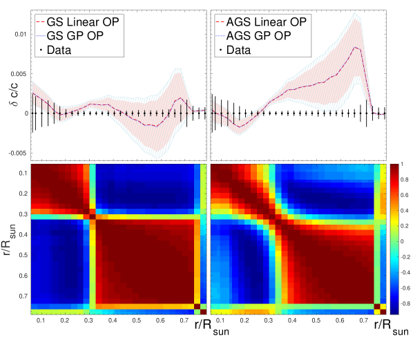
In Fig. 2 we plot the fractional sound speed difference $\delta c(r)\equiv(c_{\rm obs}(r)-c(r))/c(r)$, where $c_{\rm obs}(r)$ is the sound speed inferred from helioseismic data while $c(r)$ represent the sound speed profile predicted by the B16-GS98 (left) and B16-AGSS09met (right) model, respectively. The blue (lighter) hatched area and the red (darker) shaded area corresponds to the 1$\sigma$ theoretical uncertainties in sound speed predictions obtained for linear and GP opacity uncertainty priors. As seen from the figure, and expected from the comparison of the top panels in Fig. 1, they are not very different in the two considered cases. Moreover, we observe from the figure that at almost all radii, independently of the adopted prescription, the sound speed profile of B16-GS98 fits well within the 1$\sigma$ data uncertainties. It may be thus surprising that the B16-GS98 model is not providing a good p-value in the case of linear opacity uncertainty parametrization.

The reason for the bad p-value obtained for the B16-GS98 model is that, as discussed in Vinyoles et al. (2017), changes in input quantities do not lead to variations in SSM sound speeds on very small radial scales, so values of the sound speed at different radii in solar models are strongly correlated, i.e. the model correlation matrix $\rho_{{\rm mod},ij}$ in Eq. (9) is highly non-diagonal. This is shown in the lower panels of Fig. 2 where we graphically display the values for the entries of the correlation matrix between the predicted sound speeds at the 30 locations (the correlation matrix is the same for both B16 models). As seen in the figure, the characteristic correlation length (i.e. the distance $|r_{i}-r_{j}|$ over which correlations between the predicted values of the sound speeds are strong, say $|\rho_{{\rm mod},ij}|\gtrsim 0.5$) is much larger for the linear opacity profile parametrization than for the GP profile.

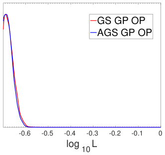
The more flexible implementation of the opacity profile uncertainty provided by the GP procedure permits to obtain a better description of the observational data for both B16-GS98 and B16-AGSS09met models. To illustrate this point, Fig. 3 shows the posterior distribution of $L$, the correlation length hyperparameter (Eq. (15)). As seen from the figure, the best possible description of the data is achieved with correlation lengths of average $\langle L\rangle\sim 0.2$, i.e. close to the lowest value permitted by the adopted prior that allows for short scale modifications of the sound speed profiles.

Figure 2: $1\sigma$ range of variation of the fractional sound speed profiles as predicted by the priors the B16 SSM models and for both opacity profile priors discussed in the text (upper panels) compared with the 30 data points used in the analysis. The lower panels graphically display the values of the entries in the $30\times 30$ model correlation matrix between between the predicted sound speeds at the 30 points (which are the same for B16-GS98 and B16-AGSS09met models) for the linear opacity uncertainty parametrization (left) and the GP opacity uncertainty(right).

We finish this section by giving in Table 3 the Bayes factors for the two models as obtained with their posterior probability distributions after including the neutrino and helioseismic data for the two assumed opacity profile uncertainties. From the table we conclude that the B16-AGSS09met models are always somewhat disfavoured with respect to the B16-GS98 model by all data sets but the most statistical significant effect is driven by the sound speed profile data. This is particularly the case for the linear opacity uncertainty profile for which the Bayes factor of -14.7 is enough for rejection of the model. Allowing for the most flexible GP form of the opacity uncertainty decreases the evidence against the B16-AGSS09met model to close to strong.

	B16-AGSS09met/B16-GS98
Data	LIN-OP	GP-OP
$\nu$	-0.23	-0.27
+$Y_{S}$+$R_{CZ}$	-1.6	-2.2
+ sound speeds	-14.7	-4.1

Table 3: Bayes factor, $\ln(\mathcal{B})$, for the B16-AGSS09met vs B16-GS98 model obtained with the different data sets (see table 1 for interpretation).

Figure 3: Posterior probability distribution for the correlation length hyperparameter $L$ of the GP opacity uncertainty for runs with the models B16-GS98 and B16-AGSS09met priors for the abundances.

5 Determination of the Optimum Composition and Opacity Profile

We now turn to the determination of the optimum solar composition which best describes the helioseismic and neutrino data. In order to do so we perform Bayesian parameter inference by using a top hat prior for the logarithmic abundances $\varepsilon_{i}\equiv\log_{10}(N_{i}/N_{\rm H})+12$ that accommodates both the AGSS09met and GS98 admixtures, i.e. with value 1 between the $3\sigma$ lower value of the AGSS09met composition and the $3\sigma$ upper value of the GS998 composition for all the nine elements relevant for solar model construction given in Tab. 4, and zero outside this range. As before we study the dependence of our results on the two models for the opacity uncertainty.

Figure 4: Posterior probability distribution for the logarithmic abundances ($\varepsilon_{j}-\varepsilon_{j,\rm GS98})$ from the analysis of neutrino and helioseismic data with uniform priors for the abundances and for the two choices of the prior opacity uncertainties. The distributions are given in arbitrary units and they have been normalized in such a way that the maximum of all distributions lays at the same height. See text for details.

Figure 5: Graphical representation of correlations between the posterior distributions of individual elemental abundances (elements in the same order as in Table 4) for the linear (left) and GP (right) models of intrinsic opacity uncertainty.

Element	GS98	AGSS09met	Linear	GP
C	$8.52\pm 0.06$	$8.43\pm 0.05$	[8.32, 8.56]	[8.31, 8.51]
N	$7.92\pm 0.06$	$7.83\pm 0.05$	[7.88, 8.10]	[7.81, 8.05]
O	$8.83\pm 0.06$	$8.69\pm 0.05$	[8.82, 8.91]	[8.80, 8.94]
Ne	$8.08\pm 0.06$	$7.93\pm 0.10$	[7.87, 8.06]	[7.90, 8.16]
Mg	$7.58\pm 0.01$	$7.53\pm 0.01$	[7.54, 7.60]	[7.52, 7.58]
Si	$7.56\pm 0.01$	$7.51\pm 0.01$	[7.57, 7.59]	[7.54, 7.59]
S	$7.20\pm 0.06$	$7.15\pm 0.02$	[7.35, 7.38]	[7.27, 7.37]
Ar	$6.40\pm 0.06$	$6.40\pm 0.13$	[6.14, 6.44]	[6.20, 6.50]
Fe	$7.50\pm 0.01$	$7.45\pm 0.01$	[7.42, 7.44]	[7.42, 7.48]
CNO	$9.04\pm 0.04$	$8.92\pm 0.03$	[9.03, 9.08]	[9.00, 9.09]
meteor.	$8.09\pm 0.01$	$8.04\pm 0.01$	[8.08, 8.10]	[8.07, 8.10]

Table 4: 1-$\sigma$ ranges for the logarithmic abundances $\varepsilon_{j}$. The first two columns show the mean values and uncertainties of the GS98 and AGSS09met heavy element admixtures. The last two columns give the ranges of the posterior distributions from the analysis of neutrino and helioseismic data for the two choices of the prior opacity uncertainties with uniform priors for the abundances.

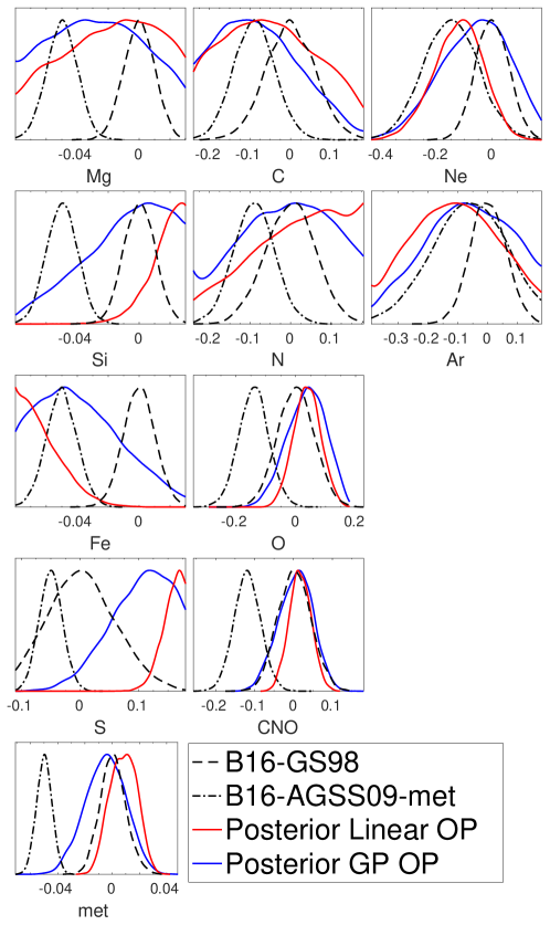
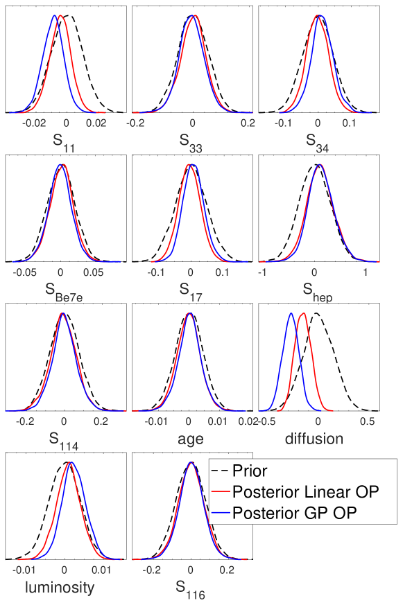
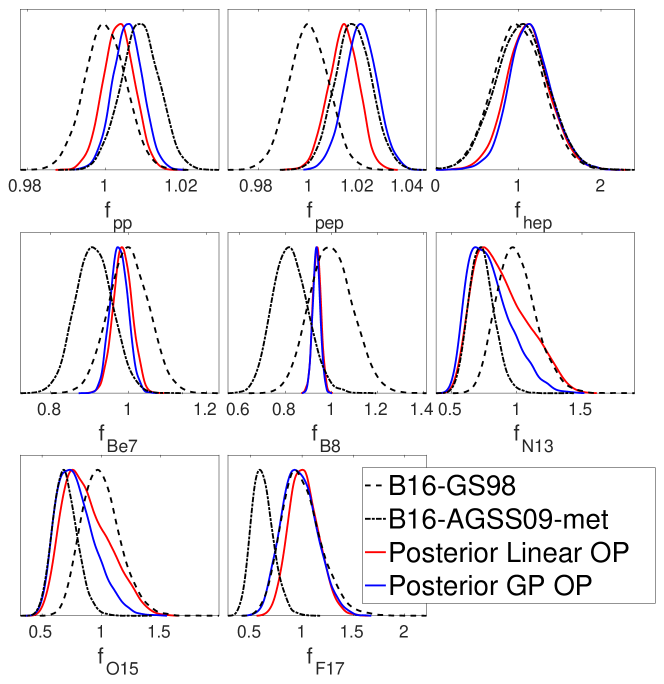
We show in Fig. 4 the posterior probability distributions for the nine abundance parameters centered for reference around the GS98 ones, i.e. $\Delta\varepsilon_{j}=\varepsilon_{j}-\varepsilon_{j,\rm GS98}$, and for the two choices of priors of the opacity uncertainties (Linear or GP). The window for each abundance corresponds to the allowed range, i.e. where prior=1. Outside each window the value of the prior is zero. For the sake of comparison we also show in the figure the corresponding prior distributions for the B16-GS98 and B16-AGSS09met models. Notice that the distributions are given in arbitrary units and have been normalized in such a way that the maximum of all distributions lays at the same height to help comparison.

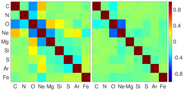
We list in the last two columns of Table 4 the corresponding $\pm 1$-$\sigma$ ranges for the logarithmic abundances $\varepsilon_{j}$ extracted from these posterior distribution. These can be compared with the determination of the same quantities in GS98 and AGSS09met compilations reported in the first two columns of the same table. From the figure and table we see that the available data are not capable of setting tight constraints on all the elements simultaneously. However we find that the posterior for the combinations of CNO (C+N+O) and meteorite (Mg+Si+S+Fe) abundances (Delahaye & Pinsonneault, 2006; Villante et al., 2014) have a comparable precision to GS98 and AGSS09met observational determinations for either choice of the opacity uncertainty parametrization. It is important to stress here that the distributions for these combinations have been obtained without assuming any prior correlation between the individual elements. This is in contrast to previous work (Delahaye & Pinsonneault, 2006; Villante et al., 2014), where abundances of all elements within a group were forced to have the same proportional change. Correlations among the posterior distributions of the abundances appear exclusively as output of the data analysis. For the sake of illustration we provide in Fig. 5 a graphic representation of the correlation among the posterior probability distributions of the different elemental abundances. As expected, the correlations are smaller for the run with the more flexible GP description of the opacity profile uncertainty. But in general for both GP and Linear opacity uncertainties, the correlation among the posterior distributions of the abundances included either the CNO or the meteorite groups are not very large. The exception is provided by the large anticorrelation between the posterior distributions of C and O for the analysis with Linear opacity uncertainty. We have verified that because the allowed ranges of C and O are strongly anticorrelated in this case, the allowed range of CNO group abundance results to be more precise than any of the model priors as seen in the lower central panel in Fig. 4.

The posterior distributions for the other solar input parameters – luminosity, diffusion, age, and the eight nuclear rates, are shown in Fig. 6 together with their gaussian priors. From the figure we see that with the exception of $S_{11}$ and diffusion coefficients, all others parameters do not get significantly modified with respect to the model priors by the inclusion of the neutrino and helioseismic data, irrespective of the form of the opacity uncertainty. We have verified that the helioseismic data – the surface helium abundance $Y_{\rm S}$ and the location of the bottom of the convective envelope $R_{\rm CZ}$ – are the most relevant in driving the shift in $S_{11}$. We see from the figure that the posterior distributions for $S_{11}$ show a preferred value about 1% lower than our prior central value taken from (Marcucci et al., 2013) and 1.5% lower than the newer determination of $S_{11}$ by (Acharya et al., 2016). A reassessment of this relevant rate might be therefore important. The sound speed data are instead responsible for the preference of lower values of the diffusion coefficients. The reduction in diffusion efficiency that we obtain is in line with previous work (Villante et al., 2014). Our analysis, however, points towards a $30\pm 10$% reduction, larger in comparison with 12% found in (Villante et al., 2014) and closer to 21% found in (Bahcall et al., 2001).

Figure 6: Posterior probability distribution for the Sun luminosity, Sun diffusion, the Sun age, and the eight nuclear rates from the analysis of neutrino and helioseismic data with uniform priors for the abundances and for the two choices of the prior opacity uncertainties. For comparison we also show their prior distribution. The distributions are given in arbitrary units and they have been normalized in such a way that the maximum of all distributions lay at the same height.

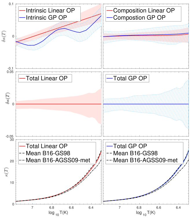
The posterior distributions for the opacity profiles are shown in Fig. 7. In the upper left panel, we plot the 1$\sigma$ range of the intrinsic opacity change $\delta\kappa_{I}(T)$. This is obtained from the posteriors of the parameters characterizing this function, i.e. the parameters $a$ and $b$ for the linear opacity parametrization given by Eq. (13), and the 11 values $\delta\kappa_{Ii}=\delta\kappa_{I}(T_{i})$ that sample the function $\delta\kappa_{I}(r)$ (after marginalizing over the correlation length $L$) for GP. By construction, the intrinsic opacity change $\delta\kappa_{I}(T)$ is defined with respect to a reference opacity calculation $\overline{\kappa}(\rho,T,Y,Z_{i})$ that in our analysis include the atomic opacities from OP (Badnell et al., 2005) complemented at low temperatures by molecular opacities from (Ferguson et al., 2005). The fact that the posterior distribution of $\delta\kappa_{I}(T)$ is not centered at zero (and, moreover, individuates a trend as a function of $T$) indicates that there are features of the observational data, namely the wiggle in the sound speed profile for $0.3<r/R_{\odot}<0.6$, that cannot be optimally fitted by using the reference opacities, even with the freedom of varying the solar input parameters within their uncertainty ranges and the solar composition in a large intervals considered in this paper, that accommodate both AGSS09met and GS98 observational results. The preference for a slight modification of the OP opacity is consistent with what found in (Villante et al., 2014) where indeed it was emphasized that the sound speed is better fitted by using the old OPAL opacity tables.

As explained in Sec. 3.3, the quantity that is directly constrained by observational data is the SSM opacity profile $\kappa_{\rm SSM}(T)$, defined according to Eq. (17), that is affected by composition modifications (and solar model recalibration) in addition to the effects of the intrinsic opacity change $\delta\kappa_{I}(T)$. In the lower panels of Fig. 7, we show the posterior distributions for $\kappa_{\rm SSM}(T)$ for the linear (left) and GP (right) description of opacity uncertainty. The posterior distributions for $\kappa_{\rm SSM}(T)$ are compared with the opacity profiles of B16-GS98 and B16-AGSS09met models. We see that they are almost coincident with the the opacity profile of B16-GS98 model, as it is expected by considering that the best fit CNO and meteoritic elemental abundances, that drive the change in the opacity, are close to GS98 determinations. The optimal opacity profile is well defined by observational data, as it is seen in the central left (right) panels of Fig. 7 where we show the $1\sigma$ relative dispersion of $\kappa_{\rm SSM}(r)$ with respect to its mean posterior value. The uncertainty for $\kappa_{\rm SSM}(r)$ is somewhat larger for the GP opacity uncertainty description, ranging from 0.8% at the center to 4% at the base of the convective envelope, while for the linear uncertainty parameterization it varies from 0.5% to 2.5%.

Finally, we note that the uncertainty in $\kappa_{\rm SSM}(r)$ is smaller than that of the intrinsic opacity change. In fact, $\delta\kappa_{I}(r)$ is not directly constrained by the observational properties of the Sun and its determination suffers from the degeneracy with the composition opacity change $\delta\kappa_{\rm Z}(T)$ that is quantified by Eq. (21). For completeness, we report in the upper (right) panel of Fig. 7, the $1\sigma$ range for the composition opacity change $\delta\kappa_{Z}(r)$, obtained from Eq. (20) with $\delta z_{j}$ being the variance of the posterior distributions of the abundances in Fig. 4 defined relative to the mean of those posteriors. Being defined with respect to the mean of the posterior, the corresponding $\delta\kappa_{Z}$ are centered around zero.

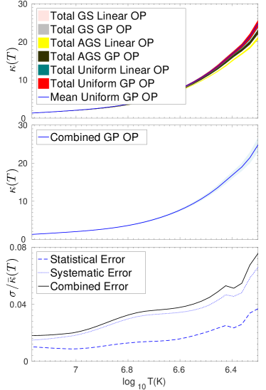
The result obtained with the uniform composition and with GP opacity uncertainty prior represents our best estimate of the radiative opacity profile in the solar interior. On the other hand, the profiles obtained with other choices of priors, such us the uniform composition with linear opacity uncertainty, or the four cases with B16-GS98 and B16-AGSSmet composition priors with either choice of the opacity uncertainty prior presented in Sec. 4, can serve as a measure of the systematic uncertainty in this estimate that reflects dependence on the choice of priors. We show in the top panel in Fig. 8 the 1$\sigma$ range of the posteriors for these six priors. From those we construct a systematic uncertainty in the opacity, at each temperature, defined as the standard deviation of the six reconstructed opacity profiles. The final opacity profile with both error sources added in quadrature is shown in the central panel in Fig. 8 and it ranges from 2% at the center to 7.5% at the bottom of the convective zone.

Figure 7: Posterior distribution for the opacity profiles for the analysis with uniform priors for the abundances and the two choices of priors of the opacity uncertainties. See text for discussion.

Figure 8: Top: 1$\sigma$ ranges for the posteriors of the opacity profiles corresponding to the six choice of priors for the composition and intrinsic uncertainty variation used in this work. Central: Posterior distribution for the opacity profiles for the analysis with uniform priors for the abundances and the GP opacity uncertainty. The panel shows the mean and 1$\sigma$ range of this distribution combining both statistical and systematic uncertainties. Lower: The panel shows its “statistical” 1$\sigma$ uncertainty defined as the corresponding variance of the posterior (shown also as “total” in the central right panel in Fig. 7) and its “systematic” uncertainty defined defined as the standard deviation of the six profiles shown on the top window.

Finally, for completeness, we show the resulting posterior distribution for the neutrino fluxes in Fig. 9. By construction they constitute the predicted solar neutrino fluxes by models which better describe both the helioseismic and neutrino data. We denote them as helioseismic and neutrino data driven fluxes, B17-HNDD. We list in Table 5 their best values and 1$\sigma$ uncertainties and in Eq. (22) their correlations.

$$\rho=\left(\begin{tabular}[]{cccccccc}1.00&0.80&0.03&-0.41&-0.02&-0.27&-0.27&0.12\\ 0.80&1.00&0.06&-0.33&-0.05&-0.28&-0.29&0.01\\ 0.03&0.06&1.00&-0.01&-0.01&-0.02&-0.02&0.01\\ -0.41&-0.33&-0.01&1.00&0.13&-0.03&-0.02&-0.03\\ -0.02&-0.05&-0.01&0.13&1.00&0.04&0.06&0.06\\ -0.27&-0.28&-0.02&-0.03&0.04&1.00&0.99&-0.14\\ -0.27&-0.29&-0.02&-0.02&0.06&0.99&1.00&-0.12\\ 0.12&0.01&0.01&-0.03&0.06&-0.14&-0.12&1.00\\ \end{tabular}\right)$$ (22)

Figure 9: Posterior distributions for the neutrino fluxes for the analysis with uniform priors for the abundances and the two choices of priors of the opacity uncertainties. For the sake of comparison we show the corresponding priors for the B16-GS98 and B16-AGSS09met models. The distributions are given in arbitrary units and they have been normalized in such a way that the maximum of all distributions lay at the same height. The fluxes are shown normalized to the B16-GS98 prediction $f_{i}=\phi_{i}/\phi_{i}^{\rm B16-GS98}$.

B17-HNDD $\nu$-Fluxes
$\Phi({\rm pp})$	$6.017\,(1^{+0.0033}_{-0.0041})$
$\Phi({\rm pep})$	$1.470\,(1\pm 0.0061)$
$\Phi({\rm hep})$	$9.04\,(1^{+0.22}_{-0.21})$
$\Phi({\rm{}^{7}Be})$	$4.79\,({1^{+0.027}_{-0.019}})$
$\Phi({\rm{}^{8}B})$	$5.10\,(1\pm 0.018)$
$\Phi({\rm{}^{13}N})$	$1.89\,(1^{+0.32}_{-0.14})$
$\Phi({\rm{}^{15}O})$	$1.50\,(1^{+0.23}_{-0.20})$
$\Phi({\rm{}^{17}F})$	$4.90\,(1^{+0.22}_{-0.18})$

Table 5: Posterior solar neutrino fluxes for uniform-GP models. Units are: $10^{10}$ (pp), $10^{9}$ (⁷Be), $10^{8}$ (pep, ¹³N, ¹⁵O), $10^{6}$ (⁸B, ¹⁷ F) and $10^{3}$(hep) cm⁻²s⁻¹.

As expected, we find that for those neutrino fluxes which are at present most precisely determined in solar neutrino experiments, ⁸B and ⁷Be, the B17-HNDD flux is very close to their experimental value used to construct the neutrino data part of the Likelihood function (see last column in table 6) but with a smaller uncertainty because of the additional indirect constraints imposed by the helioseismic data. Interestingly we find that with the inclusion of the helioseismic data the precision of the predicted B17-HNDD CNO fluxes is only at most a factor ${\cal O}(2)$ weaker than those of the B16-GS98 or B16-AGSS09met composition models.

6 Summary

In this work we have used Bayesian parameter inference and Gaussian process for non-parametric functional reconstruction of the radial opacity profile, with the goal of making an statistically consistent use of the information from helioseismic and neutrino observations for solar modeling. In particular to better determine the solar chemical composition and other solar properties (as well as their uncertainties) which are relevant to the solar composition problem.

In Secs. 2 and  3 we have presented a brief summary of the statistical methodology followed and the application of Gaussian process for functional reconstruction, and in particular to the radial opacity profile parametrization. Sections  4 and  5 contain our results which we can be summarized as follows:

• B16-GS98 vs B16-AGSS09met comparison. This improves over results in (Vinyoles et al., 2017) because the linear parametrization of opacities was not flexible enough. Now GP adds more flexibility to the models so our results are now more general and much less dependent on the choice of opacity tables. Helioseismic and neutrino data favors the B16-GS98 model over B16-AGSS09met, but the more flexible modeling of the opacity uncertainty allowed by the GP approach makes this preference less marked.

• Best composition. In our analysis all elements have uncorrelated prior distributions. Therefore, our results are more general than those from previous works (Villante et al., 2014). When considering individual elements, constraints are not very stringent on their abundances. This was expected. The best case is O, with a well defined gaussian distribution with 1$\sigma$=0.07 dex, close to the spectroscopic value. When elements are grouped as CNO or meteoritic, the posterior distributions of these groups are well peaked with uncertainties in the linear(GP) analysis of 0.025(0.045) dex and 0.01(0.015) dex respectively, comparable to those obtained from spectroscopic measurements. Due to our adoption of a flat prior for elemental abundances and our introduction of the GP approach for modeling opacity uncertainties, our results are quite general, with as little dependence on modeling assumptions as possible (e.g. the bounds in in Villante et al. 2014 are obtained in the assumption that the difference OP-OPAL is the measure of the intrinsic opacity uncertainty).

• Non-composition input parameters. The posterior distributions of these parameters have also been determined and are the most general results available to date. $S_{11}$ varies at the 1$\sigma$ level (1% with respect to (Marcucci et al., 2013) when compared to (Acharya et al., 2016). This is not a large difference, but further work on this important rate might be worth. Our best estimate of the rate of microscopic diffusion is also lower, by about 2$\sigma$, than the standard rate used in solar models. This is qualitatively expected, but the 30% reduction is quantitatively larger than previous estimates that suggested reductions in the range of 15-20% (Delahaye & Pinsonneault, 2006; Villante et al., 2014)

• Opacity reconstruction. This is the most important result of our work. We have been able to reconstruct the solar opacity profile in a data driven way, i.e. without strong assumptions on the solar composition or the underlying opacity tables. Considering uncertainties due to the solar data alone, the opacity uncertainty is about 4% at the base of the convective zone and less than 1% at the solar core. Different sets of priors help us quantify a systematic uncertainty in this estimate. From a broad range of assumptions, our more conservative estimate of the total opacity uncertainty (data + priors) is 7.5% at the base of the convective envelope and 1.8% at the solar core.

• Neutrino fluxes. We have obtained the posterior distributions of solar $\nu$-fluxes based on the uniform prior distribution of solar abundances and GP treatment of opacity uncertainties. These fluxes represent the best data driven reconstruction of the expected solar models $\nu$-fluxes. For the well measured ⁸B and ⁷Be fluxes, the final uncertainties reflect experimental uncertainties. For CN fluxes, the predicted values are approximately only a factor of 2 larger than in the B16 SSMs ($\sim$ 20-25%). This is remarkable because their uncertainty is dominated in our analysis by the C+N abundance, that has a much larger prior range of variation.

Appendix A Data included in the analysis

We construct the likelihood function with data from helioseismology and neutrino oscillation experiments. In particular we include the two helioseismic quantities widely used in assessing the quality of SSMs: the surface helium abundance $Y_{\rm S}$ and the location of the bottom of the convective envelope $R_{\rm CZ}$. In Table 6 we include the experimentally determined value for those two quantities. For illustration we also show the mean and variation of their expected values in the B16 SSM’s (which however are not directly use in building the corresponding likelihood). In building the corresponding likelihood function we assume the experimental errors to be totally uncorrelated.

Qnt.	B16-GS98	B16-AGSS09met	Solar
$Y_{\rm S}$	$0.2426\pm 0.0059$	$0.2317\pm 0.0059$	$0.2485\pm 0.0035$
$R_{\rm CZ}/{\rm R_{\odot}}$	$0.7116\pm 0.0048$	$0.7223\pm 0.0053$	$0.713\pm 0.001$
$\Phi({\rm pp})$	$5.98(1\pm 0.006)$	$6.03(1\pm 0.005)$	$5.971^{(1+0.006)}_{(1-0.005)}$
$\Phi({\rm pep})$	$1.44(1\pm 0.01)$	$1.46(1\pm 0.009)$	$1.448(1\pm 0.009)$
$\Phi({\rm hep})$	$7.98(1\pm 0.30)$	$8.25(1\pm 0.30)$	$19^{(1+0.63)}_{(1-0.47)}$
$\Phi({\rm{}^{7}Be})$	$4.93(1\pm 0.06)$	$4.50(1\pm 0.06)$	$4.80^{(1+0.050)}_{(1-0.046)}$
$\Phi({\rm{}^{8}B})$	$5.46(1\pm 0.12)$	$4.50(1\pm 0.12)$	$5.16^{(1+0.025)}_{(1-0.017)}$
$\Phi({\rm{}^{13}N})$	$2.78(1\pm 0.15)$	$2.04(1\pm 0.14)$	$\leq 13.7$
$\Phi({\rm{}^{15}O})$	$2.05(1\pm 0.17)$	$1.44(1\pm 0.16)$	$\leq 2.8$
$\Phi({\rm{}^{17}F})$	$5.29(1\pm 0.20)$	$3.26(1\pm 0.18)$	$\leq 85$

Table 6: Main characteristics for the different SSMs with the correspondent model errors and the values for the observational values and their error. For the fluxes units are: $10^{10}$ (pp), $10^{9}$ (⁷Be), $10^{8}$ (pep, ¹³N, ¹⁵O), $10^{6}$ (⁸B, ¹⁷ F) and $10^{3}$(hep) cm⁻²s⁻¹. For the fluxes the last column “Solar” corresponds to the values obtained from direct fit to the solar neutrino data in Bergström et al. (2016).

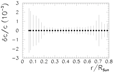
We also include the fractional sound speed differences in 30 points along the solar radius determined by performing sound speed inversions as described in (Basu et al., 2009). In Vinyoles et al. (2017) we give a detailed summary of the sources of uncertainties for the sound speed profile. These “experimental” uncertainties are conservatively assumed to be uncorrelated. For completeness we plot in Fig. 10 the fractional sound speed differences used in our statistical analysis which, by definition, have zero central values.

Finally we include the results from oscillation experiments in the form of the likelihood of the global analysis of neutrino oscillation data used and described in Bergström et al. (2016) in terms of 3-$\nu$ oscillations with arbitrary normalization of each of the components of the solar flux. For the sake of illustration we list in the last column in Table 6 the central values and errors of the solar flux normalizations extracted in that analysis. Effectively the effect of the inclusion of the neutrino oscillation data can be understood in terms of a reduced gaussian likelihood constructed with these extracted eight solar fluxes and uncertainties and with the correlation matrix:

$$\rho=\left(\begin{tabular}[]{cccccccc}1&0.99&-0.05&0.08&-0.14&-0.20&-0.19&-0.11\\ 0.99&1&-0.05&0.08&-0.14&-0.20&-0.19&-0.11\\ -0.05&-0.05&1&-0.08&0.10&-0.01&-0.00&-0.00\\ 0.08&0.08&-0.08&1&-0.17&-0.31&0.09&0.10\\ -0.14&-0.14&0.10&-0.17&1&-0.02&-0.03&-0.01\\ -0.20&-0.20&-0.01&-0.31&-0.02&0&0.18&0.09\\ -0.19&-0.19&-0.00&0.09&-0.03&0.18&1&0.36\\ -0.11&-0.11&-0.00&0.10&-0.01&0.09&0.36&1\\ \end{tabular}\right)$$ (23)

Figure 10: Fractional sound speed data $\delta c/c=(c_{\odot}-\bar{c}^{\rm mod})/\bar{c}^{\rm mod}$ used in our analysis.

Appendix B Gaussian Process for Function Reconstruction

Gaussian process (GP) is a non-parametric regression method widely used in statistics and machine learning to reconstruct a function which best describes some data without assuming a parametrization of the function (see e.g. Murphy 2012; Rasmussen & Williams 2006; Mackay 2003 or the Gaussian Process webpage for details). It is used for example in data analysis in cosmology to reconstruct some of the evolution dependent properties (like the dark energy equation of state; Holsclaw et al., 2010b, a; Seikel et al., 2012). Seikel et al. (2012) contains a pedagogical description of the process which we briefly sketch here.

The starting assumption is that the value of the function $f$ evaluated at a point $x$ is a Gaussian random variable of mean $\mu(x)$ and variance ${\rm Var}(x)$. As the values of the function in two points $x$ and $x^{\prime}$ are not independent, in general one can define a covariant function ${\rm cov}(f(x),f(x^{\prime}))\equiv C(x,x^{\prime})$. The assumed “prior” covariance function is arbitrary although the obvious hypothesis is that it depends only on the distance between the points. For example, a common choice is a square exponential

$$C_{P}(x,x^{\prime})=\sigma_{f}^{2}\,\mathrm{exp}\left(-\frac{(x-x^{\prime})^{2}}{2\lambda^{2}}\right),$$ (24)

which depends on the parameters $\sigma_{f}$ and $\lambda$, often referred to as “hyperparameters” as they do not specify the form of the function but give a measure of its characteristic variations. $\lambda$ can be seen as the characteristic length over which the function changes significantly while $\sigma_{f}$ is its range of variation at each point.

The procedure aims at determining the posterior mean and variance value of the function at some predetermined points, $f_{i}=f(x_{i})$, $i=1,N$. This is, to determine $\mu_{i}=\mu(x_{i})$ and $C_{ij}=C(x_{i},x_{j})$ starting from some prior mean function $\mu_{p}(x)$ and the chosen prior for the covariant function. It does so by finding the optimum values of $\sigma_{f}$ and $\lambda$ (or marginalizing over them) by confronting them with the data.

In the simplest case the data to be described corresponds to the value of the function at specific points $\tilde{x}_{a}$, $y_{a}=f(\tilde{x}_{a})$ with $a=1$ to $\tilde{N}$, known with some uncertainties $\sigma_{a}$ (or what is the same with some experimental covariance $\tilde{C}_{ab}$). In this case it can be shown that the likelihood for the hyperparameters takes the form

$$-2\ln\mathcal{L}(\sigma_{f},L)=$$ (25)

$$\sum_{ab=1}^{\tilde{N}}\left\{(y_{a}-\mu_{a})(C_{t})^{-1}_{ab}(y_{b}-\mu_{b})+\ln(C_{t})_{ab}\right\}+\,\rm{const}$$

where $\mu_{a}=\mu_{p}(x_{a})$ and $C_{t}=C_{P}+\tilde{C}$. The posterior mean and covariance for the function at the specific points are

$$\bar{f}_{i}=\mu_{p}(x_{i})+\sum_{ab=1}^{\tilde{N}}{C_{P}}_{ia}(C_{t})^{-1}_{ab}(y_{b}-\mu_{b})$$ (26)

$$C_{ij}={C_{P}}_{ij}-\sum_{ab=1}^{\tilde{N}}{C_{P}}_{ia}(C_{t})^{-1}_{ab}C_{bj}\,.$$ (27)

For the problem at hand, the data – neutrino fluxes, helioseismic data, and sound speeds – are functions of the opacity function that we want to determine (not some values of it) so the procedure to use Gaussian Process has to be adapted as described in Sec. 3.2

References

- Abdurashitov et al. (2009) Abdurashitov J. N., et al., 2009, Phys. Rev., C80, 015807
- Abe et al. (2011) Abe K., et al., 2011, Phys. Rev., D83, 052010
- Acharya et al. (2016) Acharya B., Carlsson B. D., Ekstr嗄 A., Forss始 C., Platter L., 2016, Phys. Lett., B760, 584
- Aharmim et al. (2013) Aharmim B., et al., 2013, Phys. Rev. C, 88, 025501
- Asplund et al. (2006) Asplund M., Grevesse N., Sauval J., 2006, Nucl. Phys., A777, 1
- Asplund et al. (2009) Asplund M., Grevesse N., Sauval A. J., Scott P., 2009, Ann. Rev. Astron. Astrophys., 47, 481
- Badnell et al. (2005) Badnell N. R., Bautista M. A., Butler K., Delahaye F., Mendoza C., Palmeri P., Zeippen C. J., Seaton M. J., 2005, Mon. Not. Roy. Astron. Soc., 360, 458
- Bahcall (1964) Bahcall J. N., 1964, Phys. Rev. Lett., 12, 300
- Bahcall & Davis (1976) Bahcall J. N., Davis R., 1976, Science, 191, 264
- Bahcall & Pinsonneault (1992) Bahcall J. N., Pinsonneault M. H., 1992, Rev. Mod. Phys., 64, 885
- Bahcall & Pinsonneault (1995) Bahcall J. N., Pinsonneault M. H., 1995, Rev. Mod. Phys., 67, 781
- Bahcall & Ulrich (1988) Bahcall J. N., Ulrich R. K., 1988, Rev. Mod. Phys., 60, 297
- Bahcall et al. (1968) Bahcall J. N., Bahcall N. A., Shaviv G., 1968, Phys. Rev. Lett., 20, 1209
- Bahcall et al. (2001) Bahcall J. N., Pinsonneault M. H., Basu S., 2001, Astrophys. J., 555, 990
- Bahcall et al. (2005a) Bahcall J. N., Basu S., Pinsonneault M., Serenelli A. M., 2005a, Astrophys. J., 618, 1049
- Bahcall et al. (2005b) Bahcall J. N., Serenelli A. M., Basu S., 2005b, Astrophys. J., 621, L85
- Bahcall et al. (2006) Bahcall J. N., Serenelli A. M., Basu S., 2006, ApJS, 165, 400
- Bailey et al. (2015) Bailey J. E., et al., 2015, Nature, 517, 56
- Basu & Antia (2008) Basu S., Antia H. M., 2008, Phys. Rept., 457, 217
- Basu et al. (2009) Basu S., Chaplin W. J., Elsworth Y., New R., Serenelli A. M., 2009, ApJ, 699, 1403
- Bellini et al. (2010) Bellini G., et al., 2010, Phys. Rev., D82, 033006
- Bellini et al. (2011) Bellini G., et al., 2011, Phys.Rev.Lett., 107, 141302
- Bellini et al. (2014a) Bellini G., et al., 2014a, Nature, 512, 383
- Bellini et al. (2014b) Bellini G., et al., 2014b, Phys. Rev., D89, 112007
- Bergström et al. (2016) Bergström J., Gonzalez-Garcia M. C., Maltoni M., Peña-Garay C., Serenelli A. M., Song N., 2016, Journal of High Energy Physics, 3, 132
- Bottino et al. (2002) Bottino A., Fiorentini G., Fornengo N., Ricci B., Scopel S., Villante F. L., 2002, Phys. Rev., D66, 053005
- Castro et al. (2007) Castro M., Vauclair S., Richard O., 2007, Astron. & Astrophys., 463, 755
- Christensen-Dalsgaard et al. (1996) Christensen-Dalsgaard J., et al., 1996, Science, 272, 1286
- Cleveland et al. (1998) Cleveland B. T., et al., 1998, Astrophys. J., 496, 505
- Colgan et al. (2016) Colgan J., et al., 2016, ApJ, 817, 116
- Cravens et al. (2008) Cravens J., et al., 2008, Phys. Rev., D78, 032002
- Delahaye & Pinsonneault (2006) Delahaye F., Pinsonneault M. H., 2006, ApJ, 649, 529
- Ferguson et al. (2005) Ferguson J. W., Alexander D. R., Allard F., Barman T., Bodnarik J. G., Hauschildt P. H., Heffner-Wong A., Tamanai A., 2005, Astrophys. J., 623, 585
- Feroz & Hobson (2008) Feroz F., Hobson M., 2008, Mon. Not. Roy. Astron. Soc., 384, 449
- Feroz et al. (2009) Feroz F., Hobson M., Bridges M., 2009, Mon. Not. Roy. Astron. Soc., 398, 1601
- Feroz et al. (2013) Feroz F., Hobson M. P., Cameron E., Pettitt A. N., 2013, preprint, (arXiv:1306.2144)
- Fiorentini et al. (2001) Fiorentini G., Ricci B., Villante F. L., 2001, Phys. Lett., B503, 121
- Gondolo & Raffelt (2009) Gondolo P., Raffelt G. G., 2009, Phys. Rev. D, 79, 107301
- Grevesse & Sauval (1998) Grevesse N., Sauval A. J., 1998, Space Sci. Rev., 85, 161
- Gribov & Pontecorvo (1969) Gribov V. N., Pontecorvo B., 1969, Phys. Lett., B28, 493
- Guzik & Mussack (2010) Guzik J. A., Mussack K., 2010, ApJ, 713, 1108
- Haxton & Serenelli (2008) Haxton W. C., Serenelli A. M., 2008, ApJ, 687, 678
- Holsclaw et al. (2010a) Holsclaw T., Alam U., Sanso B., Lee H., Heitmann K., Habib S., Higdon D., 2010a, Phys. Rev. Lett., 105, 241302
- Holsclaw et al. (2010b) Holsclaw T., Alam U., Sanso B., Lee H., Heitmann K., Habib S., Higdon D., 2010b, Phys. Rev., D82, 103502
- Hosaka et al. (2006) Hosaka J., et al., 2006, Phys. Rev., D73, 112001
- Iglesias & Rogers (1996) Iglesias C. A., Rogers F. J., 1996, ApJ, 464, 943
- Kaether et al. (2010) Kaether F., Hampel W., Heusser G., Kiko J., Kirsten T., 2010, Phys. Lett., B685, 47
- Koshio (2015) Koshio Y., 2015, in American Institute of Physics Conference Series. p. 090001, doi:10.1063/1.4915566
- Krief et al. (2016) Krief M., Feigel A., Gazit D., 2016, preprint, (arXiv:1603.01153)
- Mackay (2003) Mackay D. J. C., 2003, Information Theory, Inference and Learning Algorithms
- Marcucci et al. (2013) Marcucci L. E., Schiavilla R., Viviani M., 2013, Physical Review Letters, 110, 192503
- Mikheev & Smirnov (1985) Mikheev S. P., Smirnov A. Yu., 1985, Sov. J. Nucl. Phys., 42, 913
- Mondet et al. (2015) Mondet G., Blancard C., Cossé P., Faussurier G., 2015, ApJS, 220, 2
- Murphy (2012) Murphy K. P., 2012, Machine learning: a probabilistic perspective
- Peña-Garay & Serenelli (2008) Peña-Garay C., Serenelli A., 2008, preprint, (arXiv:0811.2424)
- Pontecorvo (1968) Pontecorvo B., 1968, Sov. Phys. JETP, 26, 984
- Rasmussen & Williams (2006) Rasmussen C. E., Williams C. K. I., 2006, Gaussian Processes for Machine Learning
- Ricci & Villante (2002) Ricci B., Villante F. L., 2002, Phys. Lett., B549, 20
- Seikel et al. (2012) Seikel M., Clarkson C., Smith M., 2012, JCAP, 1206, 036
- Serenelli et al. (2009) Serenelli A., Basu S., Ferguson J. W., Asplund M., 2009, Astrophys. J., 705, L123
- Serenelli et al. (2011) Serenelli A. M., Haxton W. C., Pena-Garay C., 2011, Astrophys. J., 743, 24
- Serenelli et al. (2013) Serenelli A., Peña-Garay C., Haxton W. C., 2013, Phys. Rev. D, 87, 043001
- Tripathy & Christensen-Dalsgaard (1998) Tripathy S. C., Christensen-Dalsgaard J., 1998, Astron. Astrophys., 337, 579
- Turck-Chieze et al. (1988) Turck-Chieze S., Cahen S., Casse M., Doom C., 1988, Astrophys. J., 335, 415
- Villante (2010) Villante F. L., 2010, ApJ, 724, 98
- Villante et al. (2014) Villante F. L., Serenelli A. M., Delahaye F., Pinsonneault M. H., 2014, ApJ, 787, 13
- Vinyoles & Vogel (2016) Vinyoles N., Vogel H., 2016, J. Cosmology Astropart. Phys., 3, 002
- Vinyoles et al. (2015) Vinyoles N., Serenelli A., Villante F. L., Basu S., Redondo J., Isern J., 2015, J. Cosmology Astropart. Phys., 10, 015
- Vinyoles et al. (2017) Vinyoles N., et al., 2017, Astrophys. J., 835, 202
- Wolfenstein (1978) Wolfenstein L., 1978, Phys. Rev., D17, 2369