Probing Subsurface Flows in Active Region NOAA 12192 - Comparison with NOAA 10486

Abstract

Active Region (AR) 12192 is the biggest AR observed in solar cycle 24 so far. This was a long-lived AR which survived for four Carrington rotations (CR) and exhibited several unusual phenomena. We measure the horizontal subsurface flows in this active region in multiple rotations using the ring-diagram technique of local helioseismology and the Global Oscillation Network Group (GONG+) Dopplergrams, and investigate how different was the plasma flow in AR 12192 from that in AR 10486. Both regions produced several high M- and X-class flares but had different CME productivity. Our analysis suggests that these ARs had unusually large horizontal flow amplitude with distinctly different directions. While meridional flow in AR 12192 was poleward that supports the flux transport to poles, it was equatorward in AR 10486. Furthermore, there was a sudden increase in the magnitude of estimated zonal flow in shallow layers in AR 12192 during the X3.1 flare, however, it reversed direction in AR 10486 with X17.2 flare. These flow patterns produced strong twists in horizontal velocity with depth in AR 10486 that persisted throughout the disk passage as opposed to AR 12192, which produced a twist only after the eruption of the X3.1 flare that disappeared soon after. Our study indicates that the sunspot rotation combined with the re-organization of magnetic field in AR 10486 was not sufficient to decrease the flow energy even after several large flares that might have triggered CMEs. Furthermore, in the absence of sunspot rotation in AR 12192, this re-organization of magnetic field contributed significantly to the substantial release of flow energy after the X3.1 flare.

1 Introduction

During the course of each solar activity cycle, hundreds of ARs form and decay with time. These regions are responsible for producing energetic events, e.g., flares and coronal mass ejections (CMEs), thus, known as the major drivers of space weather. Observations show that a significant number of CMEs originate from flares (Yashiro et al., 2006). There are further evidences that big ARs are generally formed during the declining phase of the cycle and produce more flares and CMEs than in ascending and maximum activity periods. Many authors have investigated the possible relationships between flare properties and the CMEs physical parameters (Compagnino et al., 2017, and references therein), and also tried to determine the flare characteristics that may lead to the CME production (Liu et al., 2016, and references therein). In general, big ARs do produce both flares and CMEs. However, there are few examples where large regions did produce flares but no CMEs.

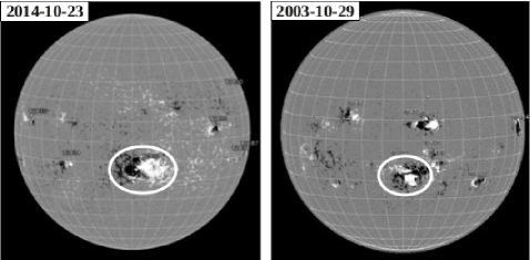
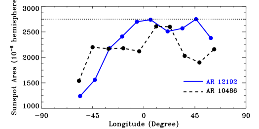
Figure 1: (Top): Magnetograms showing AR 12192 (left: from SDO/HMI) and AR 10486 (right: from SOHO/MDI) near the central meridian in Solar Cycles 24 and 23, respectively. These regions are marked by white circles. (Bottom): Temporal evolution of sunspot area in both ARs during their disk passage (Source: NOAA/SWPC). Dotted line indicates the maximum area acquired by AR 12192.

The most recent example is the NOAA 12192, the biggest AR in last 25 years which produced significant number of flares during its disk passage. However, only one small CME was reported to originate from this region. In total, there were total 73 C-class, 35 M-class and 6 X-class flares during 14 days of the disk passage (ftp://ftp.swpc.noaa.gov/pub/warehouse/). Among them, the most intense flare produced was X3.1 on 2014 October 24. In contrast to AR 12192, the biggest AR of Solar Cycle 23, AR 10486, produced 16 C-class, 16 M-class, 7 X-class flares (including X17.2 flare on 2003 October 28) and several associated halo CMEs (https://cdaw.gsfc.nasa.gov/CME_list/). In Figure 1, we show sample magnetograms of 12192 (top left) and AR 10486 (top right) around the same location on the solar disk but almost 11 years apart. The lower panel illustrates the variation of sunspot area in AR 10486 and 12192 as these pass through the Earth-facing side of the Sun. It can be seen that AR 12192 was much bigger in size than AR 10486.

Since the appearance of AR 12192, several studies have been carried out to explore its properties (Chen et al., 2015; Sun et al., 2015; Jiang et al., 2016; Liu et al., 2016; Inoue et al., 2016). However, these were confined to studying the magnetic conditions during the X3.1 flare with a focus on understanding its CME-poor nature. Sun et al. (2015) found a weaker non-potential core region in AR 12192 with stronger overlying fields, and smaller flare-related field changes when compared with other major flare-CME-productive ARs 11158 and 11429 of Cycle 24. By studying various magnetic indices, they further added that the large amount of magnetic free energy in AR 12192 did not translate into the CME productivity. The strong confinement from the overlying magnetic field responsible for the poor CME production was also confirmed by Chen et al. (2015). In a different study, Jing et al. (2015) also compared the characteristics of the X3.1 flare of AR 12192 with the X2.2 flare of CME-productive AR 11158 in terms of magnetic free energy, relative magnetic helicity and decay index of these ARs. The major difference between them was found to lie in the time-dependent change of magnetic helicity of the ARs. AR 11158 showed a significant decrease in magnetic helicity starting 4 hours prior to the flare, but no apparent decrease in helicity was observed in AR 12192. By studying decay index, these authors also confirmed the earlier findings of Sun et al. (2015) and Chen et al. (2015) that the strong overlying magnetic field was mainly responsible for low-CME productivity in AR 12192. In order to provide more insight on this, Liu et al. (2016) suggested that the large ARs may have enough current and free energy to power flares, but whether or not a flare is accompanied by a CME is related to the presence of a mature sheared or twisted core field serving as the seed of the CME, or a weak enough constraint of the overlying arcades. In a recent study, by analyzing SDO/HMI, SDO/AIA and Hinode/SOT observations, Bamba et al. (2017) studied the X1.0 flare that occurred in the same region on 2014 October 25, which also did not trigger any CME. They found that reversed magnetic shear at the flaring location was responsible for this 3-ribbon flare, and the closed magnetic field overlying a flux rope did not reach the critical decay index that prohibited the CME eruption.

Despite many studies describing the properties of AR 12192 above the solar surface, none has been published so far on the subsurface characteristics. There are no well-defined parameters from helioseismic studies that favor the CME-poor or CME-rich nature of any AR. However, in order to explore the subsurface signatures of eruptive events, Reinard et al. (2010) studied the temporal changes in subsurface helicity preceding AR flaring. Tripathy et al. (2008) also investigated the changes in acoustic mode parameters before, during, and after the onset of several halo CMEs. They found that the CMEs associated with a low value of magnetic flux regions have line widths smaller than the quiet regions, implying the longer life-time for oscillation modes. However, an opposite trend was found in the regions of high-magnetic field which is a common characteristic of the ARs (Jain et al., 2008). Both these studies were based on limited samples of ARs, hence a general conclusion was not achieved.

In this paper, we study subsurface flows associated with AR 12192 and compare with those in AR 10486. We also investigate the differences between them in order to understand the CME-poor nature of AR 12192. The paper is organized as follows; the observations of AR 12192 in multiple CRs are described in Section 2. We briefly describe the ring-diagram technique in Section 3, and subsurface flows in AR 12192 and their comparison with AR 10486 in Section 4. We discuss possible scenario supporting different characteristics of both ARs in Section 5, and finally our results are summarized in Section 6.

2 Observations

2.1 Early observations of AR 12192 in EUV

Two ARs, NOAA 12172 and 12173, appeared near the east limb in CR 2155. These regions were formed on the backside of the Sun and were closely located. Continuous observations show that both regions survived till they reached the west limb, however, AR 12173 decayed within a few days after crossing the limb while AR 12172 went through rapid evolution. The AR 12172 was later labeled as AR 12192 after its appearance on the east limb in CR 2156. To track the growth and decay of AR 12172 and AR 12173, respectively, in particular on the invisible surface the the Sun, we use “all Sun” EUV Carrington maps as described in Liewer et al. (2014). These maps are produced by combining EUV frontside images from Atmospheric Imaging Assembly (AIA) on board Solar Dynamics Observatory (SDO) with the backside images from Solar Terrestrial Relations Observatory (STEREO).

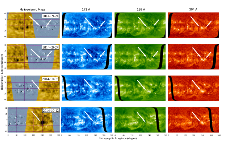
Figure 2: (left) Composite ”All Sun” Carrington maps of farside helioseismic images (yellow) and frontside line-of-sight magnetograms (grey), and corresponding maps in three EUV lines: (2nd left column) 171Å, (3rd left column) 195Å  and (right) 304Å. The location of AR 12192 is marked by the large arrow in each panel. Panels in first two rows have small arrows showing the location of AR 12173 which decayed after crossing the western limb. Following the standard practice adopted by the NOAA, AR 12192 was identified as AR 12172 in CR 2155.

In Figure 2, we show sample helioseismic and corresponding EUV maps in 195Å, 171Å and 304Å,  and for four days. The helioseismic maps are the composite images of the far- and near-side solar hemispheres, where the near hemisphere is represented by the line-of-sight magnetic field and the farside by an image showing sound wave travel time variations. The locations of shorter travel times are darker regions indicating the locations of high-magnetic field concentration on the farside. The top two rows provide maps when AR 12172 and 12173 were present on the front side, and bottom two rows for those days when they crossed the west limb. Similar to travel time maps, the high magnetic field regions in EUV images can easily be determined in the form of brightening in these images. It should be noted that communications with the STEREO Behind spacecraft were interrupted on 2014 Oct 1 that hampered the required telemetry of the data. Nevertheless, a few images from STEREO do exist that indicate the decay of AR 12173 between Sept 27 and Oct 5. A closer inspection of the images on Sept 24 (Top row) clearly shows two well-developed ARs in both photospheric magnetogram (last column) and EUV observations while in 2nd row, showing observations for Sept 27, we notice dimming in the brightness of one AR. This kind of reduction in EUV brightness is generally referred to as the decaying phase of the AR or the depletion of magnetic field strength. We further notice that only one AR was present in EUV images on Oct 5 indicating that AR 12173 was completely decayed by this time. Although there is a gap in the STEREO observations between Oct 5 and Oct 12, the helioseismic maps strongly support the rapid growth of a strong magnetic field region on the farside which is discussed below. This region could not be further tracked in EUV due to the interrupted communications with STEREO Behind spacecraft.

2.2 AR 12192 in multiple Carrington rotations - helioseismic imaging

Direct and continuous observations of the visible surface and the helioseismic far-side imaging suggest that the AR 12192 was a long-lived active region. A careful examination of these images clearly indicates that the AR survived at least for four CRs and went through various evolutionary phases. Although this is the biggest region of the current solar cycle till date, it did not produce the largest flare of the cycle or any CME. Since NOAA assigns new numbers to all ARs whenever these appear on the east limb irrespective of their reappearance after completing a solar rotation, the far-side images are crucial to ascertain the life of such ARs. The reliability of far-side images of ARs was tested in a series of papers by Liewer et al. (2012, 2014) where helioseismic farside maps were compared with backside images of the Sun from NASA’s STEREO mission. They found that approximately 90% of the helioseismic active-region predictions matched with the activity/brightness observed in EUV at the same locations. It should be noted that despite providing reasonable information on the existence of ARs in the non-earth facing side of Sun, the current method of helioeseimic imaging has a limitation on sensing strong signal near the limb. However, the signal becomes stronger when the ARs move towards the far-side central meridian.

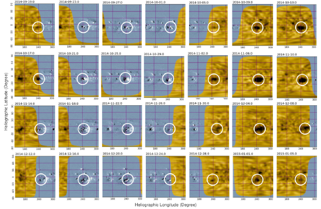
Figure 3: Far- and near-side images of AR 12192 in four consecutive CRs: CR 2155 (Top row), CR 2156 (2nd row), CR 2157 (3rd row) and CR 2158 (bottom row). Different NOAA numbers were assigned to the AR in each CR. These images are produced by the farside pipeline of SDO/HMI and are available at http://jsoc.stanford.edu/data/farside/. The existence of AR 12192 is marked by white circle in each image. Note that the AR disappeared after crossing the western limb in CR2158. Gray portions in images display the front-side line-of-sight magnetic field while yellow regions illustrates the far-side helioseismic maps. The farside maps produced by the NSO/NISP pipeline using GONG Dopplergrams (available at http://gong2.nso.edu/products/) also display similar results. Dates corresponding to these maps are given at the top of each panel.

In Figure 3, we show the images of AR 12192 in four consecutive CRs (CR 2155 - 2158) by including images of both visible and invisible surfaces. Here we shown images for every fourth day with each row corresponding to AR’s appearance in the next CR. The region of interest is marked by the white circle. Daily helioseismic maps of far side are available at http://jsoc.stanford.edu/data/farside/ using HMI and http://gong2.nso.edu/products/ using GONG observations. The evolution of AR 12192 in multiple CRs is summarized in Table 1.

3 Data and Technique

We utilize 1k $\times$ 1k continuous Doppler images from GONG at a cadence of 60 s. Although better spatial resolution space observations from MDI on board SOHO during the Dynamics run from 1995 – 2010 (1k $\times$ 1k at a cadence of 60 s) and from HMI on board SDO (4k $\times$ 4k at a cadence of 45 s) are available since 2010, the GONG observations provide a unique advantage in this work. All these instruments use photospheric lines; the GONG and MDI observations are in the Ni I 6768Å line as opposed to HMI observations in Fe I 6173Å line. Although the inference of subsurface flow should not be influenced by the spectral line used in observations (Jain et al., 2006), the different spatial resolution may introduce some bias on the results mainly due to the sensitivity to different mode sets for inversion (Jain et al., 2013a). In addition, every instrument has some type of systematic effects, thus the use of consistent data for both ARs as well as quiet regions will minimize instrument related bias, if any. Furthermore, the GONG observations will allow us to use the same quiet region values from the deep minimum phase between cycles 23 and 24 as reference. It is worth mentioning that there have been changes in the GONG instrumentation over the period of this analysis, however these were limited to adding new capabilities only, e.g., the modulator upgrade in 2006 to obtain high-cadence magnetograms and adding H-$\alpha$ filter in 2010 at a 20 s cadence for space weather studies, thus the Doppler observations were not affected. Therefore, the GONG network provides unique consistent data set of continuous high-cadence and high-spatial resolution Dopplergrams for last one and half solar cycles that can be used to study long-term solar variability.

We use the technique of ring diagrams (Hill, 1988) to study the subsurface plasma flow in AR 12192 in multiple CRs. This method has been used in numerous studies to investigate the acoustic mode parameters beneath ARs (Rajaguru et al., 2001; Tripathy et al., 2012; Rabello-Soares et al., 2016) as well as long-term and short-term variations in near-surface flows (Komm et al., 2015; Greer et al., 2015; Bogart et al., 2015; Howe et al., 2015; Tripathy et al., 2015; Jain et al., 2015). It is widely understood that the strong concentration of magnetic field alters the behavior of acoustic waves by absorbing their power. As a result, the inferences in these regions often encounter with large uncertainties. In a recent study, the credibility of the ring-diagram method was tested by comparing near-surface flows with the surface flows in three ARs calculated from ring-diagram and the local correlation tracking methods, respectively (Jain et al., 2016). The authors reported a good correlation between these two quantities. Studies further show that the uncertainties in inferences tend to increase towards the limb (Jain et al., 2013b), hence our analysis is restricted to within $\pm$45${\arcdeg}$ from the disk center.

In the ring-diagram method, high-degree waves propagating in localized areas over the solar surface are used to obtain acoustic mode parameters in the region of interest. In this work, we track and remap the regions of $15^{\arcdeg}\times 15^{\arcdeg}$ (128 $\times$ 128 pixels in the spatial directions) for 1664 min (referred to as 1 ring day) at the surface rotation rate (Snodgrass, 1984). The tracking rate of each central latitude in these regions is of the form cos($\theta$)[$a_{0}+a_{2}$sin${}^{2}(\theta)+a_{4}$ sin${}^{4}(\theta)$], where $\theta$ is the latitude and the coefficients $a_{0}$ = 451.43 nHz, $a_{2}$ = $-$ 54.77 nHz, and $a_{4}$ = $-$ 81.17 nHz. We then apodize each tracked area with a circular function and a three-dimensional FFT is applied in both spatial and temporal directions to obtain a three-dimensional power spectrum that is fitted using a Lorentzian profile model (Haber et al., 2002),

$$P(k_{x},k_{y},\omega) = {A\over(\omega-\omega_{0}+k_{x}U_{x}+k_{y}U_{y})^{2}+\Gamma^{2}}+{b\over k^{3}}$$ (1)

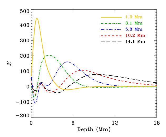
Figure 4: Representative averaging kernels used in the RLS inversion as a function of depth. The centroids of these kernels are located at depths mentioned in the figure. The kernels become less localized with the increase in centroids’ depths.

where $P$ is the oscillation power for a wave with a temporal frequency ($\omega$) and the total wave number $k^{2}=k_{x}^{2}+k_{y}^{2}$. There are six parameters to be fitted: two Doppler shifts ($k_{x}U_{x}$ and $k_{y}U_{y}$) for waves propagating in the orthogonal zonal and meridional directions, the background power ($b$), the mode central frequency ($\omega_{0}$), the mode width ($\Gamma$), and the amplitude ($A$). Finally, frequencies along with the fitted velocities ($U_{x}$ and $U_{y}$) and formal errors are used as input to a regularized least square (RLS) method to estimate depth dependence of various components of the horizontal velocity (zonal: $V_{x}$ and meridional: $V_{y}$). While the zonal component provides an estimate of the flow in east-west direction, the meridional component is for the north-south direction. The depth dependences of mode kernels used in the inversion are shown in Figure 4. It can be seen that the kernels sharply peaks near the surface due to the availability of large modes for the kernel construction, however as the centroids of the kernels increases in depth, the kernels become broader and the inversion’s depth resolution becomes poorer.

In order to investigate the subsurface variability with the evolution/decay of ARs, we use quiet region values as a reference and subtract them from the AR values in various time samples. Our analysis is restricted to radial order $n$ = 0 – 6 in the frequency range of 1700$\mu$Hz $\leq\nu\leq$ 5200$\mu$Hz. It should be noted that we have used custom patches processed through the latest version of the GONG ring-diagram pipeline (version 3.6.1). Although both active regions studied in this paper were located close to the multiple of $7^{\arcdeg}.5$ in both directions (the grid spacing used in ring-diagram pipeline), the standard products provided different locations for AR 10486 on the solar disk from those for AR 12192. Hence, for the direct comparison between these ARs, we have customized the time series in AR 10486 which means the start and end times for each set are different from the standard products.

3.1 Quantitative estimates of magnetic activity

In our study, we also quantify the magnetic activity in various regions by calculating the Magnetic Activity Index (MAI) in each sample using the line-of-sight magnetic field from the magnetograms. Here we convert magnetogram data to absolute values, average over the length of a ring day and apodise them into circular areas to match the size of the Dopplergram patches used in the ring-diagram analysis. We use both SOHO/MDI and GONG magnetograms to calculate MAI. Since the entire period under study is not covered by the MDI magnetograms alone, we use the 96 minute MDI magnetograms for 2003 and GONG magnetograms sampled every 32 minutes for 2008 and 2014. Lower threshold values of 50 and 8.8 G are used for MDI (Basu et al., 2004) and GONG (Tripathy et al., 2015), respectively, which are approximately 2.5 times the estimated noise in the individual magnetograms. In addition, we also correct the magnetic field data from space for cosmic-ray strikes. To generate a uniform set of MAIs, the MDI MAI values are scaled to GONG values using a conversion factor of 0.31, which was obtained by relating the line-of-sight magnetic field measurements between these two instruments using a histogram-equalizing technique (Riley et al., 2014).

4 Results

4.1 Systematics and the selection of quiet regions

In a study of the subsurface characteristics of any active region in multiple time samples, the first step is to eliminate the influence of systematic effects, if any. The most common error comes from the foreshortening that may arise due to the change in heliographic locations of the tracked regions during the disk passage. To overcome this effect, we calculate reference values of quiet regions at the same heliographic locations as the AR and subtract them from the AR values as described in Jain et al. (2012, 2015). As a result, we obtain residuals that provide estimates of flows due to the change in magnetism. Another problem is the selection of quiet regions which may also influence the inferences. Tripathy et al. (2009) have examined the role of the choice of quiet regions in helioseismic studies and demonstrated that the results derived for the pairs of quiet and ARs were biased by the selection of quiet regions. They further suggested that an ensemble average of quiet regions should be used in such studies.

In previous studies, we have chosen quiet regions from the neighboring Carrington rotations (Jain et al., 2012, 2015). However, for an unbiased comparison between ARs 12192 (CR 2155) and 10486 (CR 2009), we use same quiet regions from the deep minimum phase between cycles 23 and 24 for both ARs. Note that this was the period of extremely low solar activity, hence the values obtained with reference to this period can be termed as “true” AR values. Although, both ARs appeared in two different solar cycles, this selection of quiet regions is supported by the following observational facts; (i) both ARs were observed in same phase of the year when the values of the solar inclination angle ($B_{0}$) were comparable, and (ii) both ARs were located around the same latitude in the southern hemisphere (Figure 1). Thus the projection effect in both cases can be uniformly removed by using the same quiet-region values. The period of 2008 September thru December is used to determine the quiet-region values.

We compute error-weighted averages of the MAIs for 13 ring days (approximate time for any region to cross the disk) at each heliographic location. Since we are interested in studying the temporal variation in the subsurface properties of AR 12192 in four CRs and $B_{0}$ varies from +7${\arcdeg}$.0 (September) to $-$1${\arcdeg}$.5 (December) during the period of analysis, the quiet regions are selected in such a way that the values of MAI do not significantly change from region to region. Average MAIs for quiet regions at 15 disk positions along latitude 15${\arcdeg}$ for four different ranges of $B_{0}$ are summarized in Table 2. The $B_{0}$ values chosen here correspond to those for the active regions analyzed in this paper. The regions along the latitude 15${\arcdeg}$ are separated by 7${\arcdeg}$.5 and cover the solar surface from $60{\arcdeg}$E to $60{\arcdeg}$W. It can be seen that the MAIs vary from 0.3 to 0.6 G and the standard deviation is within 18% with largest values near the limb decreasing to about 8% near central meridian.

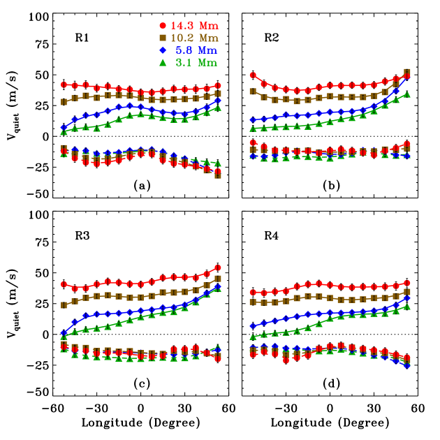
Figure 5: Variation of error-weighted averages of zonal (solid) and meridional (dashed) components of the horizontal velocity as a function of disk location at 4 target depths during the minimum activity period in 2008. Symbols represent the calculated values while lines represent for the 3-point running mean. Each panel corresponds to a fixed range of $B_{0}$; (a) R1: 7^°.05 – 6^°.51, (b) R2: 5^°.31 – 3^°.99, (c) R3: 2^°.58 – 0^°.91, and (d) R4: $-$0^°.69 – $-$2^°.39. These four ranges of $B_{0}$ correspond to the data obtained from 2008 September to 2008 December.

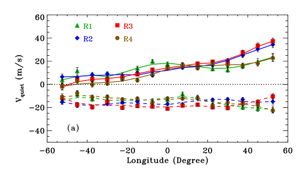
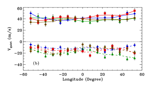
Figure 6: Variation of error-weighted averages of zonal (solid) and meridional (dashed) components of the horizontal velocity as a function of disk location at fixed depths (a) 3.1 Mm and (b) 14.3 Mm. Symbols represent the calculated values while lines are for the 3-point running mean of the calculated values in different ranges of $B_{0}$; R1: 7^°.05 – 6^°.51, R2: 5^°.31 – 3^°.99, R3: 2^°.58 – 0^°.91, and R4: $-$0^°.69 – $-$2^°.39. These four ranges of $B_{0}$ correspond to the data obtained from 2008 September to 2008 December.

We further calculate the components of horizontal velocity corresponding to these quiet regions and compute error-weighted averages of 13 ring days at each location as for MAIs. As our selected regions have an overlap of 7${\arcdeg}$.5, we smooth these components with 3-point running mean which are later used as reference in the active-region analysis. The longitudinal variation of these components across the disk is displayed in Figure 5 where different panels represent the averages for different $B_{0}$ ranges at four target depths below the surface, i.e. 3.1, 5.8, 10.2 and 14.2 Mm. It is clearly seen that the magnitude of $V_{x}$ increases with depth which is in agreement with the observations where rotation rate is found to increase with depth in the outer 5% of the Sun. There are some variations in the magnitude of $V_{y}$ as well, however these are within 1$\sigma$. Further, both zonal and meridional velocities show an east-west trend but it is more prominent in the zonal component. Also, the shallower layers are more affected by this systematic, which decreases with depth. To highlight the variation in east-west trend with time, we plot, in Figure 6, the variation of both components with disk location at depths 3.1 Mm and 14.2 Mm. We notice significant variations in these components with both time and depth. These systematics were also noticed by Zhao et al. (2012) in the the time-distance analysis where they found both travel-time magnitude and variation trends to be different for different observables. Though these authors did not provide any physical basis for this effect, they suggested that these systematics must be taken into account for the accurate determination of flows. Later, Baldner & Schou (2012) explained this effect in terms of highly asymmetrical nature of the solar granulation which results in the net radial flow. This east-west trend was also studied by Komm et al. (2015) in flows from the ring-diagram analysis for both GONG and HMI observations, where different data sets exhibited different systematics. They concluded that the trends could be removed adequately by selecting reference values from the same data source. Thus, in our study of the temporal variation of flows at different depths, we use reference values that depend on both depth and the disk location of the active region.

4.2 AR 12192 and subsurface horizontal flows

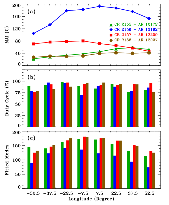
Figure 7: (a) Temporal variation of magnetic activity index (MAI) in AR 12192 in four consecutive CRs. Note that different NOAA numbers are assigned to the same region in different CR, (b) histogram showing the duty cycle corresponding to each region, and (c)the number of fitted modes used in inversion to calculate the depth-dependence of flow fields. Note that the histograms are shown at fixed eight locations as described in text.

Manifestation of strong magnetic fields is not only visible on the solar surface and beyond in the solar atmosphere, it also has significant influence on the subsurface properties. While most acoustic mode parameters tend to change linearly with the increase or decrease in magnetic field strength (Tripathy et al., 2015, and references therein), the velocity vectors have a complex relationship. These are modified in the presence of strong fields, however there are several other factors that may dominate amplitude and the direction of velocity vectors. In general, the topology of ARs plays an important role in defining the velocity components. Also, moderately large number of modes are needed in inversion for reliably calculating the depth dependence of flows. The evolution or decay of the magnetic activity in AR 12192 in multiple CRs is illustrated in Figure 7. Locations of the reference image (i.e. the image at the center of each timeseries) are given in Table 3. Since the Carrington longitude identifies the unique location of any region on the solar surface, we have made sure that it does not change with time. The heliographic location for this AR is 247${\arcdeg}$.5 longitude and $-15^{\mathrm{o}}$ latitude. It can be seen that the magnetic field strength in this AR became stronger in the second rotation (CR 2156) which decayed to a moderate level in third rotation (CR 2157). It further decayed in the fourth rotation and the MAI values became comparable to those in the first rotation (CR 2155).

Among additional factors that may influence the inference of flow vectors, the high duty cycle is crucial in obtaining reliable flows. The large gaps in observations or low duty cycle reduce the number of fitted modes that have significant effect on the inverted flows and produce large errors. Since the duty cycle in GONG observations varies from day-to-day, primarily due to the changing weather conditions at observing sites or to system maintenance/breakdown, the results may be altered. To authenticate our results, we also include duty cycles in Table 3 and Figure 7 for each timeseries. It can be seen that these are $\geq$ 70% in all time series which is above the lower threshold set in earlier studies (R. Komm, private communication). The mean duty cycles for eight ring days in each CR are 88.0%, 85.4%, 91.8% and 88.3% with the variation between 1.2$\sigma$ to 2.3$\sigma$ within the CR. Another factor is the heliographic location of the region which also influences the number of modes. Thus, fitted modes are predominantly governed by all three factors; higher magnetic field, low duty cycle and the larger distance from disk center lead to a lower number of fitted modes. It is evident from the lower panel in Figure 7 that the number of modes in CR 2156 at each location is relatively low though the duty cycles at some locations are comparable to other CRs. This clearly demonstrates the effect of the significantly strong magnetic field in CR 2156 on the acoustic modes, which reduces their amplitude and as a result, produces large errors. We estimate the variation in number of modes is less than 2$\sigma$ in each CR which is higher than the variation in duty cycle.

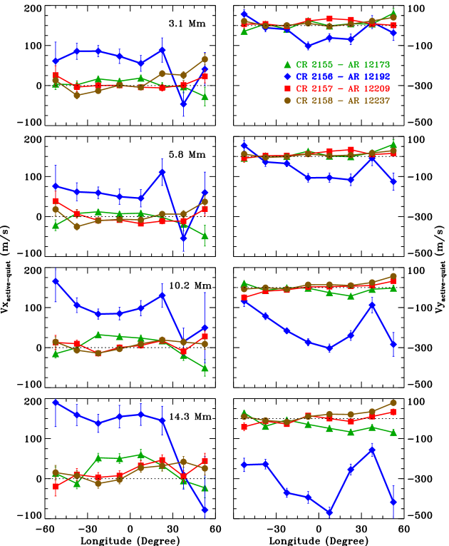
Figure 8: Temporal variation of zonal (left) and meridional (right) components of the horizontal velocity below AR 12192 in four CRs at four depths below the surface. The uncertainties in velocity determination in all rotations except CR 2156 are smaller than the size of the symbols. Note that the velocity ranges are different for both zonal and meridional components.

Temporal variation of $V_{x}$ and $V_{y}$ for the AR in each CR are displayed in Figure 8. These values are obtained by subtracting the quiet Sun values at the same locations. In the absence of any high magnetic field region, the meridional component is typically poleward (negative values in the southern hemisphere) that provide basis for the magnetic flux transport from low latitudes to the poles, and the zonal component is in the direction of solar rotation. However, as mentioned above, their amplitudes as well as directions are modified due to the change in the characteristics of AR. We obtain maximum values of both velocity components in CR 2156 in comparison to other three CRs. It is further noted that the values of both components are comparable (within 1$\sigma$) in shallow layers in all CRs except CR 2156, however these differ moderately in deeper layers. We also find very large flows in deeper layers in CR 2156. Since the MAI values are significantly large in CR 2156 (Figure 7), these could be responsible for the large flows and different behavior in this Carrington rotation. We also notice exceptionally large errors at $\pm$52${\arcdeg}$.5 in CR 2156 that may arise due to lower number of modes available for inversion as shown in Figure 7.

4.3 Comparison with AR 10486

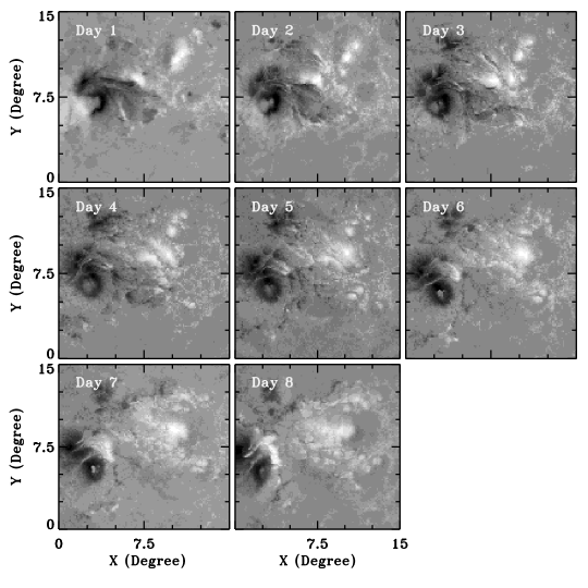
Figure 9: SDO/HMI magnetograms showing the evolution of AR 12192 in $15^{\arcdeg}\times 15^{\arcdeg}$ tiles for eight consecutive ring days in CR 2156. The locations of these regions are described in Table 3.

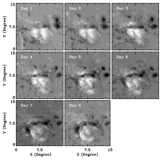
Figure 10: SOHO/MDI magnetograms showing the evolution of AR 10486 in $15^{\arcdeg}\times 15^{\arcdeg}$ tiles for eight consecutive ring days in CR 2009. The locations of these regions are described in Table 4.

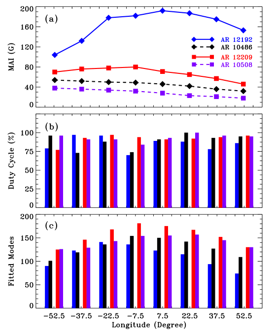
Figure 11: (a) Temporal variation of magnetic activity index (MAI) in AR 12192 (12209) and AR 10486 (10508) for two consecutive CRs are shown by solid and dashed lines, respectively. Note that different NOAA numbers are assigned to these ARs in next CRs and these are in parenthesis, (b) histogram showing the duty cycle corresponding to each region, and (c) the number of fitted modes used in inversion to calculate the depth-dependence of flow fields. Note that the histograms are shown at fixed eight locations as described in text, and AR 12192 (12209) and AR 10486 (10508) are grouped together for comparison at each location.

The active region 10486 was a long-lived AR (González Hernández et al., 2007) that produced several X- and M-class flares and associated CMEs in cycle 23. The magnetic classification of this region was similar to AR 12192, however the field strength was not as strong as it was in AR 12192. There was a slow decrease in the magnetic field in AR 10486 in the next CR while it decreased significantly in AR 12192. In order to compare the horizontal flows from both active regions, the position of ARs in the tracked cubes is crucial. If one region is off centered from the other, the inferences of mode parameters and the flows will be biased by the area covered. Further, quiet areas within the tile will modify the results as calculated flows are averaged over the entire tile. To reduce the biasing of these factors, as mentioned in Section 3, both regions are tracked at the Snodgrass rotation rate which allows us to cover the same area in tracking ensuring that the ARs stay at the same location in the tracked cube. Sample images of the evolution of ARs 12192 and 10486 in the tracked cubes for eight consecutive ring days are shown in Figures 9 and 10, respectively. These are the magnetogram regions near or at the reference image which is the center of the each time series. Since both ARs are large, it is clearly visible that these cover a reasonably large area of the tracked regions with stable positions of ARs within the tiles. The start and end of each time series representing AR 12192 and AR 10486 at different disk locations are listed in Tables 3 and 4, respectively. Temporal variations of MAI, duty cycle and the number of fitted modes in both regions for two consecutive CRs are displayed in Figure 11. As illustrated, the number of modes in AR 12192 and 10486 were comparable in the first two days and then differences started to arise which increased as ARs moved towards the west. These differences may introduce some bias in the flow estimates and the errors are also large when different mode sets are available for inversion. For convenience, in the following analysis, we will refer to regions in different CRs by their NOAA numbers. We, therefore, compare the subsurface properties of AR 12192 with those of AR 10486, and AR 12209 with AR 10508 in the next rotation.

Figure 12 illustrates the daily variation of zonal and meridional velocities. Our analysis reveals a number of similarities as well as differences between ARs 12192 and 10486. We find that both ARs maintained significantly large flows during their disk passages but distinctly different directions. Locations of X3.1 and X17.2 flares in ARs 12192 and 10486, respectively are also marked in Figure 12 and also tabulated in Tables 3 and 4. The resultant amplitude of both components is found to increase with depth. While there is a small change in $V_{x}$ in AR 12192 several days before the X3.1 flare, the gradient is sharp in the case of AR 10486. In fact, direction was reversed in AR 10486 a day before the flare around 6 Mm producing a twist in the horizontal velocity, whose amplitude continued to increase with time. Interestingly, there was an increase in $V_{x}$ in AR 12192 at the time of X3.1 flare which then decreased significantly with a small twist near the surface despite producing another X2.0 flare. Furthermore, the calculated meridional components showed a different trend; although there was a small temporal variation in AR 10486, the maximum values in AR 12192 in deeper layers were achieved a day before the X3.1 flare with the decreasing trend after that.

Figures 13a and 13b illustrate the depth variation of estimated total horizontal velocity at eight disk locations where each panel represents an individual ring day. It is evident that there are strong twists in the flows for AR 10486 and that the pattern persists for the first five days. Previous studies show that this kind of twist is generally associated with strong flares. As indicated in Table 4, there were a series of X- and M-class flares from this AR before and after the major X17.2 flare on Day 4, which we find to be responsible for the observed twists for several days. Note that there was X8.3 flare on Day 8 that started near the end of time series used in the analysis but continued beyond the end time. We find a slight twist near the surface in this case too but a complete flow pattern associated with this flare was not achieved. Nevertheless, the twist appears in AR 12192 on Day 7 only after the X3.1 flare despite the fact that there were other major flares before and after this event (see Table 3). Our analysis suggests that the twist disappeared thereafter when the region was centered at longitude 52^°5W. It is clear from Figure 11 that the number of fitted modes depends on the location of the region on the solar disk, decreasing as the AR moves away from the disk center making the inferences noisier with higher uncertainties. In addition, any magnetic field within the region and the duty cycle influence this number. Further, the outer boundary of the reliable inferences depends on the spatial resolution of input Dopplergrams and the GONG resolution puts this limit at around 45^° in either direction (Jain et al., 2013b). However, we have plotted flows at 52^°5W to understand their behavior after large flares, where we find the twist has disappeared and the values are expected to be biased by moderately large uncertainties. In next CRs, as evident from Figure 12, there was a significant decrease in the flow amplitude in both ARs.

5 The plausible scenario

It is believed that the magnetic fields are generated in a thin layer at the base of convection zone, known as the tachocline, hence the subsurface properties may provide useful information on their evolution. The techniques of local helioseismology are widely used to obtain vital information from the convection zone beneath quiet as well active regions. In last couple of decades, with the availability of high-resolution continuous observations at high cadence, it has become possible to map plasma flow in the convection zone and derive quantities that are directly linked with the measurements on the surface (Komm & Gosain, 2015). Further, Komm et al. (2012, and references therein) carried out several studies on a large sample of ARs to understand the overall behavior in their evolutionary and decaying phases. In addition, helioseismic studies describing subsurface characteristics beneath individual ARs are also available (Zhao & Kosovichev, 2003; Komm et al., 2008; Jain et al., 2012; Zhao et al., 2014; Jain et al., 2015). All these studies converge to a common conclusion that the magnetic regions show considerably higher subsurface velocities compared to the quiet regions and the velocities increase or decrease with the strength of magnetic elements within the region. In this study, we find significantly large velocities in ARs as compared to the quiet regions, however the quantitative measures of these velocity fields depend on various factors that are described below.

In this paper we studied two big ARs, NOAA 12192 and 10486, from two different solar cycles. There are many similarities as well as differences in the morphology of these regions. Both were large in size at the time of their appearance on the east limb and maintained a complex magnetic configuration, $\beta\gamma\delta$, throughout their disk passages. Despite being larger in size and also having stronger magnetic field than in 10486, the sunspot counts in AR 12192 were significantly lower. In contrast, AR 10486 had several rotating sunspots with high rotational velocity. These rotating sunspots are identified by their rotation around the umbral center or other sunspots within the same AR. The large positive-polarity sunspot in this region was reported to rotate uniformly at a rate of 2$\arcdeg$.67 hr^-1 for about 46 hours prior to the major flare on 2003 October 28 (Kazachenko et al., 2010). Studies show that the role of sunspot rotation in flare energetics is complex and it is often argued that the rotation of the sunspot produces energy and magnetic helicity more than the non-rotating case, thus triggering large flares. Kazachenko et al. (2010) suggested that the sunspot rotation in AR 10486 contributed significantly to the energy and helicity budgets of the whole AR. They further emphasized that the shearing motions alone stored sufficient energy and helicity in AR 14086 to account for the flare energetics and interplanetary coronal mass ejection helicity content within their observational uncertainties. In our previous study, we investigated the subsurface flows in AR 11158 that had several rotating sunspots and was the source region of first X-class flare with a halo CME in cycle 24 (Jain et al., 2015). The characteristics of subsurface flows in AR 11158 are similar to those in AR 10486 reported in this paper but the amplitude is significantly lower. A series of CMEs erupted from both AR 11158 (Kay et al., 2017) and AR 10486 (Gopalswamy et al., 2005). A closer comparison of flows in AR 10486 (Figure 12) and AR 11158 (Figure 8 of Jain et al. (2015)) clearly shows that the meridional flows are more affected by the CME eruption while rotating sunspots play a critical role in defining the zonal flows. Note that first CMEs reported from ARs 10486 and 11158 were on 2003 Oct 18 and 2011 Feb 13, respectively. Thus, we obtain similar flow patterns in these two ARs. However, the flows in AR 12192 display different characteristics, which we interpret in terms of its CME-poor nature. Further, by exploiting the high spatial resolution of HMI, we also studied flows in three sub-regions within AR 11158 and found that the leading and trailing polarity regions move faster than the mixed-polarity region. Since the spatial resolution of GONG Dopplergrams does not provide sufficient modes near the surface to obtain reliable inferences in individual polarity regions, our present study is confined to the investigation of subsurface flows in ARs as a whole.

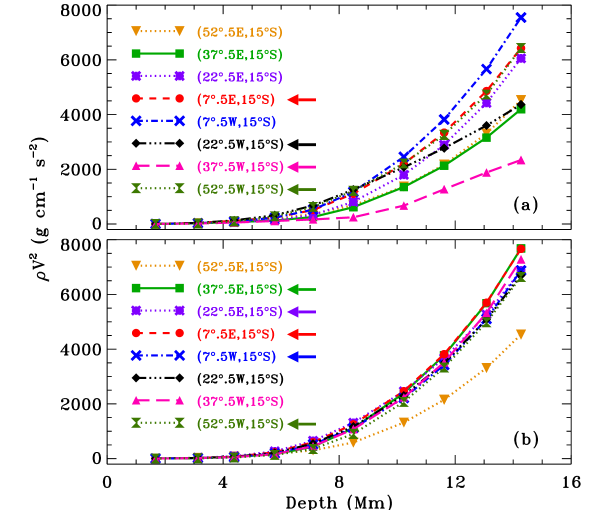
Figure 14: Depth variation of flow energy density in (a) AR 12192 and (b) AR 10486 at eight disk locations during as they move across the disk. Both ARs produced several X- and high M-class flares (see Tables 3 and 4). The regions associated with these flares are marked by arrows.

We show, in Figure 14, the depth variation of flow kinetic energy in AR 12192 and AR 10486 for 8 consecutive days when several large flares were triggered. The regions corresponding to major flares are also marked in the Figure. Here, the energy density values are calculated using the density profile in the solar interior from model “S” of Christensen-Dalsgaard et al. (1996). It can be seen that energy density increases exponentially with depth, mainly due to the rapidly increasing density. Note that these are the resultant energy density values which are elevated from the quiet region values due to the presence of high magnetic field. We notice a significant variation in energy density with time in the case of AR 12192 (upper panel) while no significant variation is seen in AR 10486 except on Day 1. It increases gradually in AR 12192 for the first 5 days although there were two large flares (M8.7 and X1.6) on Day 4. It appears that the energy released by these flares was not sufficient to disrupt the flow which eventually decreased significantly with the eruption of the X3.1 flare on Day 6. After this event, at a depth of about 13 Mm, almost 50% of the energy was dissipated which further decreased from Day 6 to Day 7 and increased from Day 7 to Day 8 with the eruption of several big flares. In all cases, this change in kinetic energy was relatively small in the upper 4 Mm. However, below this depth, there were significant changes in flow energy - from 400% around 5.8 Mm to 650% around 7.2 Mm, and this variation gradually decreased in much deeper layers. In contrast to these results, the energy variation was minimal in AR 10486, which produced several major flares on four consecutive days, including an X1.2 on Day 2, M6.7 on Day 3, X17.2 on Day 4 and X10.0 on Day 5. We believe that all these flares must have lowered the kinetic energy, however there were some other processes that rapidly supplied energy to AR 10486. Thus, the small variation in flow energy with time in AR 10486 provided favorable conditions for more energetic eruptions, e.g. CMEs in this case.

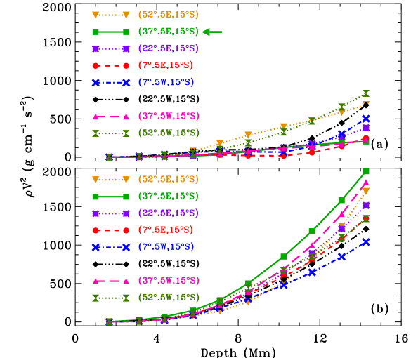
Figure 15: Depth variation of flow energy density in (a) AR 12209 (12192) and (b) AR 10508 (10486) eight disk locations during as they move across the disk. These ARs reappeared on the Earth-side limb after completing the Sun’s rotation and their NOAA numbers in the previous rotation are given in parenthesis. The AR 12209 produced a high M-class flare (see Table 3) and the region associated with this flare is marked by the arrow.

In the next rotation, as shown in Figure 15, the flow energy decreased substantially, almost by a factor of 4, in both regions. Further, the flow energy in AR 10508 (10486) is significantly higher than in AR 12209 (12192) in deeper layers while it is comparable in both regions above 4 Mm. Our study suggests that additional factors, e.g., the sunspot rotation combined with the re-organization of magnetic field in AR 10486, were not sufficient to decrease the flow energy even after several large flares and triggered CMEs. Furthermore, in the absence of sunspot rotation in AR 12192, the re-organization of magnetic field contributed significantly in the substantial release of flow energy after the X3.1 flare.

6 Summary

AR 12192 is the biggest AR observed in solar cycle 24 till date. It appeared on the east limb on 2014 October 18 and grew rapidly into the largest such region since 1990. Composite images of helioseismic farside maps and the direct frontside observations, in conjunction with STEREO and SDO/AIA EUV observations, clearly show that it was a long-lived ARs that survived at least four CRs and exhibited several unusual phenomena. Over the period of four rotations, it had the most complex magnetic configuration, $\beta\gamma\delta$, during second rotation, i.e in CR 2156 with very strong magnetic field and several large flares without any associated CMEs. We measured the horizontal subsurface flows in AR 12192 in multiple rotations applying the ring-diagram technique to the GONG+ Dopplergrams. Our analysis suggests that it had unusually large horizontal flow amplitudes before the X3.1 flare on 2014 October 24 which were comparable to those in AR 10486 during Halloween solar events in 2003. Both regions were located around the same latitude in southern hemisphere and produced several high M- and X-class flares but had different CME productivity. In order to compare the horizontal flows from both active regions, the position of ARs in the tracked cubes is crucial. If one region is off centered from the other, the inferences of mode parameters and the flows are biased by the area covered. Further, quiet areas within the tile also modifies the results as inferred quantities are averaged over the entire tile. To reduce the biasing of these factors, both regions are tracked at the Snodgrass rotation rate, which allows us to cover the same area in tracking ensuring that the ARs stay at the same location in the tracked cube. In the case of ARs 12192 and 10486, if one AR is slightly off-centered from the other AR, both cover significantly large areas of the tiles and we believe that our results are less affected by the positioning of these ARs within the tiles.

Our analysis further suggests that flow directions in these ARs were distinctly different; while meridional flow in the AR 12192 was poleward that support flux transport to the poles, it was equatorward in AR 10486. Furthermore, there was a sudden increase in the magnitude of estimated zonal flow in shallow layers in AR 12192 during the X3.1 flare, however, it reversed direction in AR 10486 with X17.2 flare. These different flow patterns provided strong twists in the horizontal velocity with depth that persisted in AR 10486 throughout the disk passage as opposed to AR 12192, which produced a twist only after the eruption of the X3.1 flare that disappeared soon after. Over the period of eight ring days, we find different flow energy patterns in these regions; there was significant variation in flow energy with time in the case of AR 12192 while no significant variation is seen in AR 10486. It increased gradually in AR 12192 for first four days until the X3.1 was produced and then declined sharply. We conclude that the sunspot rotation combined with the re-organization of magnetic field in AR 10486 was not sufficient to decrease the flow energy even after triggering several large flares that might have been responsible for CMEs. Furthermore, in the absence of rotating sunspots in AR 12192, the re-organization of magnetic field contributed significantly to the substantial release of kinetic energy after the X3.1 flare.

In future studies, we plan to identify flaring regions with and without rotating sunspots in both CME-rich and CME-poor categories to obtain a comprehensive picture linking the role of subsurface flows in the energetic eruptions. A study based on a large number of dataset may be crucial for providing subsurface thresholds for the extreme space weather events. It would also be interesting to investigate the subsurface characteristics of unique regions with CMEs but which are not associated with flares.

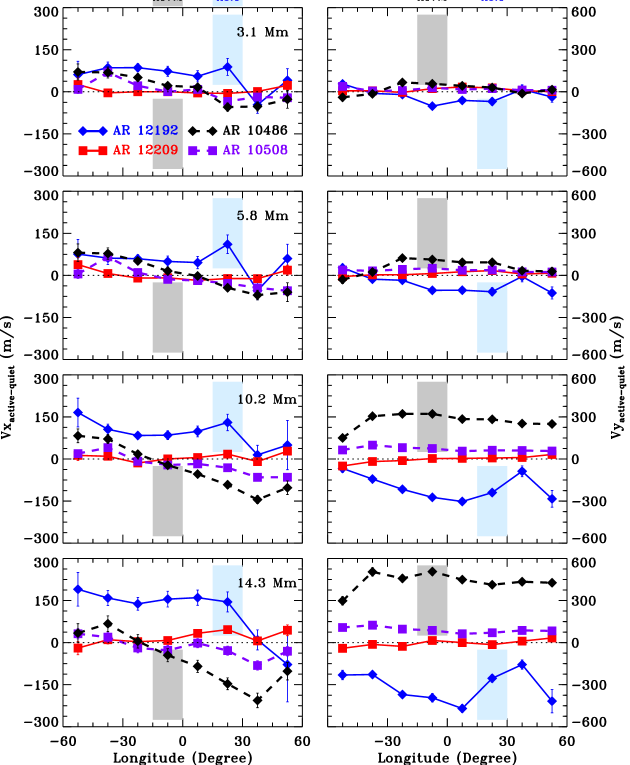
Figure 12: Temporal variation of zonal (left) and meridional (right) components of the horizontal velocity in AR 12192 (solid) and AR 10486 (dashed) in two consecutive CRs at four depths below the surface. The uncertainties in velocity determination are smaller than the size of the symbols. Note that the velocity ranges are different for both zonal and meridional components. Colored boxes show the locations of largest flares originated from these active regions.

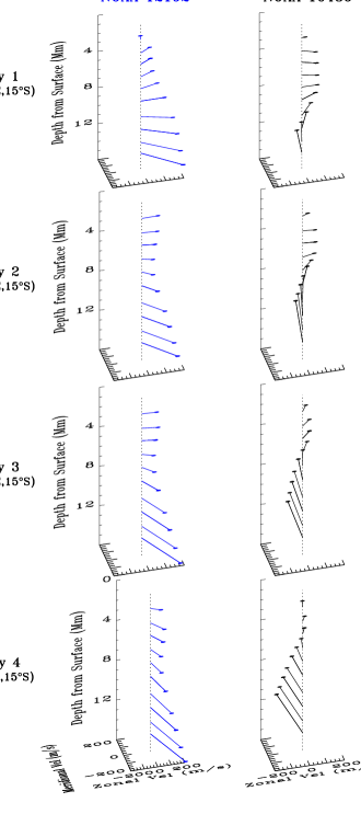
Figure 13a: Depth variation of total horizontal velocity vectors in AR 12192 (left) and AR 10486 (right) at four disk locations in eastern hemisphere in CR 2156 and 2009, respectively. Individual zonal and meridional components are plotted in Figure 12. Note that the time progresses downwards.

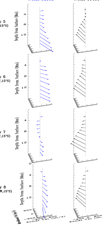
Figure 13b: Depth variation of total horizontal velocity vectors in AR 12192 (left) and AR 10486 (right) at four disk locations in western hemisphere in CR 2156 and 2009. Individual zonal and meridional components are plotted in Figure 12. Note that the time progresses downwards.

Table 1: Evolution of AR 12192 in multiple CRs. Note that different NOAA numbers were assigned to this region in each CR.

Carrington	Assigned	Number of Flares
Rotation	AR Number	C	M	X
2155	12173	19	2	0
2156	12192	73	35	6
2157	12209	33	3	0
2158	12237	3	0	0

Note. —

Table 2: Mean Magnetic Activity Index (MAI) and Standard Deviation (STDDEV) for Quiet Regions.

Reference Longitude		R1			R2			R3			R4
		MAI	STDDEV		MAI	STDDEV		MAI	STDDEV		MAI	STDDEV
(Degree)		(G)	(%)		(G)	(%)		(G)	(%)		(G)	(%)
$-$52.5		0.32	15.6		0.35	17.1		0.29	17.2		0.35	17.1
$-$45.0		0.38	13.1		0.42	14.3		0.39	12.8		0.39	12.8
$-$37.5		0.43	11.6		0.47	10.6		0.45	11.1		0.44	13.6
$-$30.0		0.48	10.4		0.50	10.0		0.50	10.0		0.43	11.6
$-$22.5		0.50	10.0		0.54	9.2		0.52	9.6		0.44	11.3
$-$15.0		0.49	10.2		0.55	9.0		0.49	10.2		0.48	10.4
$-$7.5		0.53	9.4		0.60	8.3		0.54	9.2		0.53	9.4
0		0.53	9.4		0.58	8.6		0.55	9.0		0.55	9.1
7.5		0.53	9.4		0.58	8.6		0.54	9.2		0.52	9.6
15.0		0.51	9.8		0.57	8.8		0.56	8.9		0.53	11.3
22.5		0.50	10.0		0.54	9.2		0.53	9.4		0.51	11.7
30.0		0.49	12.2		0.50	9.0		0.51	9.8		0.50	12.0
37.5		0.42	14.3		0.44	13.6		0.48	10.4		0.49	12.2
45.0		0.36	13.9		0.40	15.0		0.42	11.9		0.47	12.7
52.5		0.31	16.1		0.32	18.7		0.33	18.1		0.38	15.8

Note. — Values are given at 15^°S and 15 different locations across the disk for four ranges of $B_{0}$; R1: 7^°.05 – 6^°.51, R2: 5^°.31 – 3^°.99, R3: 2^°.58 – 0^°.91, and R4: $-$0^°.69 – $-$2^°.39. These ranges of $B_{0}$ correspond to the data obtained from 2008 September to 2008 December.

Table 3: Various regions representing AR 12192 in four rotations.

CR	AR	QR	Day		Timeseries			Location		DC
			#		Start	End		Long	Lat	(%)
2155	12172	R1
			1		2014 Sep 21 16:28UT	2014 Sep 22 20:11UT		$-$52o.5	$-$15o	86
			2		2014 Sep 22 19:44UT	2014 Sep 23 23:27UT		$-$37o.5	$-$15o	92
			3		2014 Sep 23 23:01UT	2014 Sep 25 02:44UT		$-$22o.5	$-$15o	98
			4		2014 Sep 2502:17UT	2014 Sep 26 06:00UT		$-$7o.5	$-$15o	89
			5		2014 Sep 26 05:34UT	2014 Sep 27 09:17UT		7o.5	$-$15o	84
			6		2014 Sep 27 08:51UT	2014 Sep 28 12:34UT		22o.5	$-$15o	94
			7		2014 Sep 28 12:08UT	2014 Sep 29 15:51UT		37o.5	$-$15o	77
			8		2014 Sep 29 15:24UT	2014 Sep 30 19:07UT		52o.5	$-$15o	81
2156	12192	R2
			1		2014 Oct 18 23:18UT	2014 Oct 20 03:01UT		$-$52o.5	$-$15o	79
			2		2014 Oct 20 02:36UT	2014 Oct 21 06:19UT		$-$37o.5	$-$15o	97
			3		2014 Oct 21 05:53UT	2014 Oct 22 09:36UT		$-$22o.5	$-$15o	96
			4		2014 Oct 22 09:11UT	2014 Oct 23 12:54UT		$-7$o.5	$-$15o	70
			5		2014 Oct 23 12:29UT	2014 Oct 24 16:12UT		7o.5	$-$15o	89
			6		2014 Oct 24 15:47UT	2014 Oct 25 19:30UT		22o.5	$-$15o	88
			7		2014 Oct 25 19:05UT	2014 Oct 26 22:48UT		37o.5	$-$15o	78
			8		2014 Oct 26 22:22UT	2014 Oct 28 02:05UT		52o.5	$-$15o	86
2157	12209	R3
			1		2014 Nov 15 06:32UT	2014 Nov 16 10:15UT		$-$52o.5	15o	77
			2		2014 Nov 16 09:51UT	2014 Nov 17 13:34UT		$-$37o.5	$-$15o	93
			3		2014 Nov 17 13:09UT	2014 Nov 18 16:52UT		$-$22o.5	$-$15o	97
			4		2014 Nov 18 16:28UT	2014 Nov 19 20:11UT		$-$7o.5	$-$15o	94
			5		2014 Nov 19 19:46UT	2014 Nov 20 23:29UT		7o.5	$-$15o	91
			6		2014 Nov 20 23:05UT	2014 Nov 22 02:48UT		22o.5	$-$15o	92
			7		2014 Nov 22 02:24UT	2014 Nov 23 06:07UT		37o.5	$-$15o	94
			8		2014 Nov 23 05:43UT	2014 Nov 24 09:26UT		52o.5	$-$15o	96
2158	12237	R4
			1		2014 Dec 12 14:07UT	2014 Dec 13 17:50UT		$-$52o.5	$-$15o	79
			2		2014 Dec 13 17:26UT	2014 Dec 14 21:09UT		$-$37o.5	$-$15o	83
			3		2014 Dec 14 20:46UT	2014 Dec 16 00:29UT		$-$22o.5	$-$15o	88
			4		2014 Dec 16 00:05UT	2014 Dec 17 03:48UT		$-$7o.5	$-$15o	96
			5		2014 Dec 17 03:25UT	2014 Dec 18 07:08UT		7o.5	$-$15o	97
			6		2014 Dec 18 06:44UT	2014 Dec 19 10:27UT		22o.5	$-$15o	94
			7		2014 Dec 19 10:04UT	2014 Dec 20 13:47UT		37o.5	$-$15o	93
			8		2014 Dec 20 13:23UT	2014 Dec 21 17:06UT		52o.5	$-$15o	75

Note. — The analysis is carried out using 1664 60-s Dopplergrams at each disk location. The locations are listed for the reference image which is the center image in each timeseries. Corresponding quiet region (QR) sets used in individual CRs and the duty cycle (DC) for each timeseries are also given. Regions associated with major M- ($\geq$ 5.0) and X- class flares are listed in bold.

^a M8.7 (Oct 22: 01:16UT – 02:28UT, X1.6 (Oct 22: 14:02UT – 22:30UT)

^b X3.1 (Oct 24: 20:50UT – 00:14UT), X1.0 (Oct 25: 16:55UT – 18:11UT)

^c X2.0 (Oct 26: 10:04UT – 11:18UT)

^d M7.1 (Oct 27: 00:01UT – 10:22UT), M6.7 (Oct 27: 09:59UT – 10:26UT), X2.0 (Oct 27: 14:04UT – 15:31UT)

^e M5.7 (Nov 16: 17:35UT – 17:57UT).

Table 4: Various regions representing AR 10486 in two rotations.

CR	AR	QR	Day		Timeseries			Location		DC
			#		Start	End		Long	Lat	(%)
2009	10486	R2
			1		2003 Oct 24 15:58UT	2003 Oct 25 19:41UT		-52o.5	$-$15o	96
			2		2003 Oct 25 19:16UT	2003 Oct 26 22:59UT		$-$37o.5	$-$15o	73
			3		2003 Oct 26 22:34UT	2003 Oct 28 02:17UT		$-$22o.5	$-$15o	88
			4		2003 Oct 28 01:50UT	2003 Oct 29 05:33UT		$-$7o.5	$-$15o	74
			5		2003 Oct 29 05:08UT	2003 Oct 30 08:51UT		7o.5	$-$15o	91
			6		2003 Oct 30 08:26UT	2003 Oct 31 12:09UT		22o.5	$-$15o	100
			7		2003 Oct 31 11:44UT	2003 Nov 01 15:27UT		37o.5	$-$15o	93
			8		2003 Nov 01 15:02UT	2003 Nov 02 18:45UT		52o.5	$-$15o	95
2010	10508	R3
			1		2003 Nov 20 23:22UT	2003 Nov 21 03:05UT		$-$52o.5	$-$15o	96
			2		2003 Nov 22 02:40UT	2003 Nov 23 06:23UT		$-$37o.5	$-$ 15o	91
			3		2003 Nov 23 05:58UT	2003 Nov 24 09:41UT		$-$22o.5	$-$15o	91
			4		2003 Nov 24 09:16UT	2003 Nov 25 12:59UT		$-$7o.5	$-$15o	84
			5		2003 Nov 25 12:34UT	2003 Nov 26 16:17UT		7o.5	$-$15o	93
			6		2003 Nov 26 15:52UT	2003 Nov 27 19:35UT		22o.5	$-$ 15o	100
			7		2003 Nov 27 19:10UT	2003 Nov 28 22:53UT		37o.5	$-$15o	96
			8		2003 Nov 28 22:28UT	2003 Nov 30 02:11UT		52o.5	$-$ 15o	95

Note. — The analysis is carried out using 1664 60-s Dopplergrams at each disk location. The locations are listed for the reference image which is the center image in each timeseries. Corresponding quiet region (QR) sets used in individual CRs and the duty cycle (DC) for each timeseries are also given. Regions associated with major M- ($\geq$ 5.0) and X- class flares are listed in bold.

^a X1.2(Oct 26: 06:17UT – )

^b M6.7 (Oct 27: 12:51UT -13:04UT)

^c X17.2 (Oct 28: 10:01UT – 14:20UT)

^d X10.0 (Oct 29: 20:37UT – 22:53UT)

^e X8.3 (Nov 02: 17:04UT – 19:54UT).

References

- Baldner & Schou (2012) Baldner, C. S., & Schou, J. 2012, ApJ, 760, L1
- Bamba et al. (2017) Bamba, Y., Inoue, S., Kusano, K., & Shiota, D. 2017, ApJ, 838, 134
- Basu et al. (2004) Basu, S., Antia, H. M., & Bogart, R. S. 2004, ApJ, 610, 1157
- Bogart et al. (2015) Bogart, R. S., Baldner, C. S., & Basu, S. 2015, ApJ, 807, 125
- Chen et al. (2015) Chen, H., Zhang, J., Ma, S., et al. 2015, ApJ, 808, L24
- Christensen-Dalsgaard et al. (1996) Christensen-Dalsgaard, J., Dappen, W., Ajukov, S. V., et al. 1996, Science, 272, 1286
- Compagnino et al. (2017) Compagnino, A., Romano, P., & Zuccarello, F. 2017, Sol. Phys., 292, 5
- González Hernández et al. (2007) González Hernández, I., Hill, F., & Lindsey, C. 2007, ApJ, 669, 1382
- Gopalswamy et al. (2005) Gopalswamy, N., Yashiro, S., Liu, Y., et al. 2005, Journal of Geophysical Research (Space Physics), 110, A09S15
- Greer et al. (2015) Greer, B. J., Hindman, B. W., Featherstone, N. A., & Toomre, J. 2015, ApJ, 803, L17
- Haber et al. (2002) Haber, D. A., Hindman, B. W., Toomre, J., et al. 2002, ApJ, 570, 855
- Hill (1988) Hill, F. 1988, ApJ, 333, 996
- Howe et al. (2015) Howe, R., Komm, R. W., Baker, D., et al. 2015, Sol. Phys., 290, 3137
- Inoue et al. (2016) Inoue, S., Hayashi, K., & Kusano, K. 2016, ApJ, 818, 168
- Jain et al. (2006) Jain, K., Hill, F., González Hernández, I., et al. 2006, in ESA Special Publication, Vol. 624, Proceedings of SOHO 18/GONG 2006/HELAS I, Beyond the spherical Sun, 127.1
- Jain et al. (2008) Jain, K., Hill, F., Tripathy, S. C., et al. 2008, in Astronomical Society of the Pacific Conference Series, Vol. 383, Subsurface and Atmospheric Influences on Solar Activity, ed. R. Howe, R. W. Komm, K. S. Balasubramaniam, & G. J. D. Petrie , 389
- Jain et al. (2012) Jain, K., Komm, R. W., González Hernández, I., Tripathy, S. C., & Hill, F. 2012, Sol. Phys., 279, 349
- Jain et al. (2013a) Jain, K., Tripathy, S., Basu, S., et al. 2013a, in Journal of Physics Conference Series, Vol. 440, Journal of Physics Conference Series, 012012
- Jain et al. (2013b) Jain, K., Tripathy, S. C., Basu, S., et al. 2013b, in Astronomical Society of the Pacific Conference Series, Vol. 478, Fifty Years of Seismology of the Sun and Stars, ed. K. Jain, S. C. Tripathy, F. Hill, J. W. Leibacher, & A. A. Pevtsov, 193
- Jain et al. (2015) Jain, K., Tripathy, S. C., & Hill, F. 2015, ApJ, 808, 60
- Jain et al. (2016) Jain, K., Tripathy, S. C., Ravindra, B., Komm, R., & Hill, F. 2016, ApJ, 816, 5
- Jiang et al. (2016) Jiang, C., Wu, S. T., Yurchyshyn, V., et al. 2016, ApJ, 828, 62
- Jing et al. (2015) Jing, J., Xu, Y., Lee, J., et al. 2015, Res. Astron. Astrophys., 15, 1537
- Kay et al. (2017) Kay, C., Gopalswamy, N., Xie, H., & Yashiro, S. 2017, Sol. Phys., 292, 78
- Kazachenko et al. (2010) Kazachenko, M. D., Canfield, R. C., Longcope, D. W., & Qiu, J. 2010, ApJ, 722, 1539
- Komm et al. (2015) Komm, R., González Hernández, I., Howe, R., & Hill, F. 2015, Sol. Phys., 290, 1081
- Komm & Gosain (2015) Komm, R., & Gosain, S. 2015, ApJ, 798, 20
- Komm et al. (2012) Komm, R., Howe, R., & Hill, F. 2012, Sol. Phys., 277, 205
- Komm et al. (2008) Komm, R., Morita, S., Howe, R., & Hill, F. 2008, ApJ, 672, 1254
- Liewer et al. (2014) Liewer, P. C., González Hernández, I., Hall, J. R., Lindsey, C., & Lin, X. 2014, Sol. Phys., 289, 3617
- Liewer et al. (2012) Liewer, P. C., González Hernández, I., Hall, J. R., Thompson, W. T., & Misrak, A. 2012, Sol. Phys., 281, 3
- Liu et al. (2016) Liu, L., Wang, Y., Wang, J., et al. 2016, ApJ, 826, 119
- Rabello-Soares et al. (2016) Rabello-Soares, M. C., Bogart, R. S., & Scherrer, P. H. 2016, ApJ, 827, 140
- Rajaguru et al. (2001) Rajaguru, S. P., Basu, S., & Antia, H. M. 2001, ApJ, 563, 410
- Reinard et al. (2010) Reinard, A. A., Henthorn, J., Komm, R., & Hill, F. 2010, ApJ, 710, L121
- Riley et al. (2014) Riley, P., Ben-Nun, M., Linker, J. A., et al. 2014, Sol. Phys., 289, 769
- Snodgrass (1984) Snodgrass, H. B. 1984, Sol. Phys., 94, 13
- Sun et al. (2015) Sun, X., Bobra, M. G., Hoeksema, J. T., et al. 2015, ApJ, 804, L28
- Tripathy et al. (2009) Tripathy, S. C., Antia, H. M., Jain, K., & Hill, F. 2009, in Astronomical Society of the Pacific Conference Series, Vol. 416, Solar-Stellar Dynamos as Revealed by Helio- and Asteroseismology: GONG 2008/SOHO 21, ed. M. Dikpati, T. Arentoft, I. González Hernández, C. Lindsey, & F. Hill, 139
- Tripathy et al. (2015) Tripathy, S. C., Jain, K., & Hill, F. 2015, ApJ, 812, 20
- Tripathy et al. (2012) Tripathy, S. C., Jain, K., Howe, R., Bogart, R. S., & Hill, F. 2012, Astronomische Nachrichten, 333, 1013
- Tripathy et al. (2008) Tripathy, S. C., Wet, S., Jain, K., Clark, R., & Hill, F. 2008, J. Astrophys. Astron., 29, 207
- Yashiro et al. (2006) Yashiro, S., Akiyama, S., Gopalswamy, N., & Howard, R. A. 2006, ApJ, 650, L143
- Zhao & Kosovichev (2003) Zhao, J., & Kosovichev, A. G. 2003, ApJ, 591, 446
- Zhao et al. (2014) Zhao, J., Kosovichev, A. G., & Bogart, R. S. 2014, ApJ, 789, L7
- Zhao et al. (2012) Zhao, J., Nagashima, K., Bogart, R. S., Kosovichev, A. G., & Duvall, Jr., T. L. 2012, ApJ, 749, L5