Prompt Electromagnetic Transients from Binary Black Hole Mergers

Abstract

Binary black hole (BBH) mergers provide a prime source for current and future interferometric GW observatories. Massive BBH mergers may often take place in plasma-rich environments, leading to the exciting possibility of a concurrent electromagnetic (EM) signal observable by traditional astronomical facilities. However, many critical questions about the generation of such counterparts remain unanswered. We explore mechanisms that may drive EM counterparts with magnetohydrodynamic simulations treating a range of scenarios involving equal-mass black-hole binaries immersed in an initially homogeneous fluid with uniform, orbitally aligned magnetic fields. We find that the time development of Poynting luminosity, which may drive jet-like emissions, is relatively insensitive to aspects of the initial configuration. In particular, over a significant range of initial values, the central magnetic field strength is effectively regulated by the gas flow to yield a Poynting luminosity of $10^{45}-10^{46}{\rho_{\textnormal{-}13}}{M_{8}}^{2}\,{\rm erg}\,{\rm s}^{-1}$, with BBH mass scaled to $M_{8}\equiv M/(10^{8}M_{\odot})$ and ambient density ${\rho_{\textnormal{-}13}}\equiv\rho/(10^{-13}\,{\rm g}\,{\rm cm}^{-3})$. We also calculate the direct plasma synchrotron emissions processed through geodesic ray-tracing. Despite lensing effects and dynamics, we find the observed synchrotron flux varies little leading up to merger.

I Introduction

One of the more provocative developments associated with the recent detections of gravitational waves (GWs) from mergers of stellar-mass black holes (BHs) by Advanced LIGO Abbott et al. (2016a, b) was the subsequent announcement of a possible electromagnetic (EM) counterpart signal, 0.4s after the GW150914 signal was observed. Fermi found a sub-threshold gamma-ray source in a region of the sky that overlapped the $\sim 600$-square-degree LIGO uncertainty region for GW150914 Connaughton et al. (2016). Though it may be impossible to confirm that the events are indeed physically related, the EM observation has inspired a number of papers exploring potential scenarios linking EM counterparts to stellar-mass black hole mergers Perna et al. (2016); Li et al. (2016); Zhang (2016); Loeb (2016); Morsony et al. (2016); Murase et al. (2016); Janiuk et al. (2017)—mergers that theorists had expected to be electromagnetically dark.

These events draw attention to the high potential value of multimessenger observations of GW events. While GW observations can provide extraordinarily detailed information about the merging black holes themselves, they may not provide any direct information about the black holes’ environment. Even the location of the event will be poorly determined unless an associated EM event can be identified. Such localization could also deepen our understanding of the astrophysical processes that form and influence BBH systems.

Unlike the situation for stellar-mass black holes, astronomers have long recognized the potential for EM counterparts to binary supermassive ($10^{6}$ – $10^{9}M_{\odot}$) black hole (SMBH) mergers occurring in the millihertz GW band. These mergers are a key target of future space-based GW observatories such as the LISA mission, which was recently approved by the European Space Agency Audley et al. (2017). Pre-merger GWs from these systems are a key target of nanoHertz GW searches with pulsar timing arrays Arzoumanian et al. (2014).

The large cross-section of SMBHs interacting with the ample supplies of gas common in galactic nuclear regions allows them to power some of the brightest, most long-lasting EM sources in existence, including active galactic nuclei (AGN), quasars, or radio jet emissions. A number of mechanisms may provide signals associated with these sources across a broad range of timescales from $\sim 10^{9}$ years before merger to $\sim 10^{9}$ years after merger Schnittman (2011). Considerable evidence for binary SMBH systems has already been observed, but is restricted to those either well before merger Komossa et al. (2003); Comerford et al. (2009); Smith et al. (2010); Rodriguez et al. (2006); Valtonen et al. (2008); Gabányi et al. (2016); Frey et al. (2012); Yang et al. (2017), or well after merger Merritt et al. (2004); Boylan-Kolchin et al. (2004); Gualandris and Merritt (2008); Komossa et al. (2008); Guedes et al. (2009); Batcheldor et al. (2010); Chiaberge et al. (2017).

The greatest potential for direct association with BBH mergers would come from strong EM emissions or modulations coincident with the GW event. Since LISA will observe GW emission from BBH mergers for an extended period of time, direct EM counterparts may be caused by interaction of the BBH with a circumbinary disk, perhaps during the final $\sim 10^{3}$ orbits prior to merger. Our objective, however, is to explore the mechanisms that may potentially drive EM signals directly associated with the strongest GW emissions within hours of the merger event itself. Such emissions could be crucial, for example, in LISA-based redshift-distance studies Tamanini et al. (2016).

Unlike the clean GW predictions that numerical relativity provides, one challenge of understanding EM counterpart signatures is their potential dependence on myriad details of the gas distribution, its properties, and the structure and strength of associated magnetic fields. For prompt merger-associated signals, the challenge is enhanced because the merger occurs on a very short timescale. Accretion disks, and indeed circumbinary disks, are characterized by variation over a wide range of timescales Vaughan et al. (2003); after “decoupling”, the gravitational-radiation-induced infall timescale becomes shorter than the disk accretion timescale, leading to a merger in a magnetized matter environment whose detailed structure may be impossible to predict. Even though binary torques tend to evacuate much of the surrounding region, studies in 2D & 3D reveal that dense infalling streams persist, maintaining accretion rates at levels comparable to that of a single-BH disk Farris et al. (2014); Shi and Krolik (2015).

The most valuable sort of counterpart prediction would be insensitive to these details, and have distinguishing features that clearly identify the source as a binary SMBH. While one approach to exploring this could be to seek universal features in a large number of full circumbinary-disk-plus-merger simulations, our approach here is to explore robust EM counterpart signatures from BBHs embedded in a number of simple plasma configurations.

In this paper, we employ a new tool—the IllinoisGRMHD code Etienne et al. (2015)—to study potential EM signals deriving from perhaps the simplest such initial configuration: a plasma with uniform density and magnetic fields, in which the magnetic fields are aligned with the orbital angular momentum vector.

The rest of this paper is laid out as follows. In Sec. II, we summarize relevant numerical results obtained with various methods and codes. In Sec. III, we briefly introduce our numerical code and MHD diagnostics, and compare with results from earlier work that used the WhiskyMHD code Giacomazzo et al. (2012). Section IV presents the results of our new simulations: the global state of the MHD fields (IV.1), the rate of mass accretion into the pre-merger and post-merger BHs (IV.2), the detailed behavior of the resulting Poynting luminosity (IV.3), and possible direct emission of observable photons (IV.4). We summarize our conclusions and discuss future work in Sec. V. The Appendices contain more detail on the calculation of the Poynting luminosity, effects of varying numerical resolution, and conversion between code and cgs units.

II GRMHD simulations

As dynamical, strong-field gravitational fields may drive EM counterparts to GW mergers, it is essential to build our models using the techniques of numerical relativity. Building on a revolution in methodology Pretorius (2005); Campanelli et al. (2006a); Baker et al. (2006a), numerical relativity simulations provided the first predictions Baker et al. (2006b) of astrophysical GW signals like GW150914 almost ten years before the observation. Moving beyond GW predictions in vacuum spacetimes and into EM counterpart predictions requires physics-rich simulation studies that couple the general relativistic (GR) field equations to the equations of GR magnetohydrodynamics (GRMHD), so that magnetized plasma flows in strong, dynamical gravitational fields may be properly modeled.

Over the last decade several research teams have gradually and systematically added the layers of physics necessary to begin to understand the potential for counterpart signals. Studies of test particle motion (i.e. non-interacting gases) during the last phase of inspiral and merger of MBHs showed that a fraction of particles can collide with each other at speeds approaching the speed of light, suggesting the possibility of a burst of radiation accompanying black hole coalescence van Meter et al. (2010). Other studies investigated possible EM emission from purely hydrodynamic fluids near the merging BHs O’Neill et al. (2009); Farris et al. (2010); Bode et al. (2010); Bogdanovic et al. (2011); Bode et al. (2012); Farris et al. (2011).

These studies neglected the important role that magnetic fields are likely to have in forming jets, driving disk dynamics, or in photon emission mechanisms. EM fields were first included in ground-breaking GR force-free electrodynamics (GRFFE) simulations Palenzuela et al. (2009); Palenzuela et al. (2010a); Mösta et al. (2010), investigating mergers in a magnetically dominated plasma, indicating that a separate jet formed around each BH during the inspiral. At the time of the merger, these two collimated jets would coalesce into a single jet directed from the spinning BH formed by the merger Palenzuela et al. (2010b, c); Mösta et al. (2012). Based on the black hole membrane paradigm, analysis of these studies suggested a simple formula relating the binary orbital velocity to the Poynting flux available to drive EM emissions Neilsen et al. (2011): $L_{\rm Poynt}\sim v^{2}_{\rm orbital}$.

More recent studies have begun to explore the behavior of moderately magnetized plasmas around BBH systems in an ideal GRMHD context, finding that significant EM signatures may be produced by these systems. Studies of circumbinary disk dynamics Noble et al. (2012); Farris et al. (2012); Gold et al. (2014a) have used initially circular binary BH orbits to reach a pseudo-steady state in a circumbinary disk before allowing the binary to inspiral and merge. In Gold et al. (2014b), the final merger of an equal-mass BBH was modeled in full GR, and the observed Poynting luminosity declined gradually through inspiral, only to rise significantly some time after merger.

In Giacomazzo et al. (2012) we first studied the physics of moderately magnetized plasmas near the moment of merger, using the WhiskyMHD code. Though that study was limited to just a few orbits because of technical challenges, it showed a rapid amplification of the magnetic field of approximately two orders of magnitude. This contributed to the creation, after merger, of a magnetically dominated funnel aligned with the spin axis of the final BH. The resulting Poynting luminosity was estimated to be $\sim 10^{48}\,{\rm erg}\,{\rm s}^{-1}$ (assuming an initial BBH system mass of $10^{8}\,M_{\odot}$, an initial plasma rest-mass density of $10^{-11}\,{\rm g}\,{\rm cm}^{-3}$, and an initial magnetic field strength of $\sim 10^{4}{\rm G}$). In comparison, the force-free simulations of Palenzuela et al. (2010b, c); Neilsen et al. (2011); Mösta et al. (2012) produced peak luminosities of $\lesssim 10^{44}\,{\rm erg}\,{\rm s}^{-1}$, four orders of magnitude lower than what we obtained with ideal GRMHD, despite similar initial magnetic field strengths.

These results indicate that the dynamics of BBH inspirals and mergers play an important role in driving the magnetic fields in their environment. When the BBH is embedded in an initially non-magnetically dominated plasma, accretion onto the merging BHs compresses and twists the magnetic field lines, which may strongly amplify the magnetic fields. Strengthened magnetic fields may then influence gas inflow, powering a strong EM energy (Poynting) outflow through a magnetically dominated funnel. As noted in Giacomazzo et al. (2012), such a mechanism cannot exist in the force-free regime.

Despite the ability to track GRFFE/GRMHD flows, there have been no fully GR simulations of EM counterparts to BBH mergers that actually track photons, or that could produce spectra. Instead, EM luminosity estimates have often been based on Poynting flux measurements provided directly from GRMHD fluid variables. A first step in bridging this gap was made in Schnittman (2013) using the Pandurata code Schnittman and Krolik (2013) to post-process the MHD fields around the merging binary, but assuming a fixed Kerr BH background instead of the dynamical spacetime of the GRMHD evolution itself, and also assuming a fixed electron temperature. Synchrotron, bremsstrahlung, and inverse-Compton effects combined to produce a spectrum that peaked near 100 keV. As described in Sec. IV.4, we apply a slightly more sophisticated spacetime procedure with Pandurata to obtain estimates of synchrotron luminosity and spectra from simulations presented here.

III Numerical Methods

We revisit the scenario studied in Giacomazzo et al. (2012) with fully 3D dynamical GRMHD evolutions carried out with the Einstein Toolkit Löffler et al. (2012); etk on adaptive-mesh refinement (AMR) grids supplied by the Cactus/Carpet infrastructure Schnetter et al. (2004), adopting a fully general-relativistic, BSSN-based Nakamura et al. (1987); Shibata and Nakamura (1995); Baumgarte and Shapiro (1999) spacetime metric evolution provided by the Kranc-based Husa et al. (2006) McLachlan Brown et al. (2009); mcl module, and crucially, fluid and magnetic field evolution performed with the recently released IllinoisGRMHD code Etienne et al. (2015). Initial metric data was of the Bowen-York type commonly used for moving puncture evolutions Bowen and York Jr. (1980); Brandt and Brügmann (1997), conditioned to satisfy the Hamiltonian and momentum constraints using the TwoPunctures code Ansorg et al. (2004).

The IllinoisGRMHD code is a complete rewrite of (yet agrees to roundoff-precision with) the long-standing GRMHD code used for more than a decade by the Illinois Numerical Relativity group to model a large variety of dynamical-spacetime GRMHD phenomena (see, e.g., Etienne et al. (2006); Paschalidis et al. (2011, 2012, 2015); Gold et al. (2014b) for a representative sampling). It evolves a set of conservative MHD fields $E\equiv\{\rho_{*},\tilde{\tau},\vec{\tilde{S}},\vec{\tilde{B}}\}$, derived from the primitive fields $\rho$ (baryonic density), $p$ (fluid pressure), $v^{i}$ (fluid three-velocity $\equiv u^{i}/u^{0}$, where $u^{\mu}$ is the fluid four-velocity), and $B^{i}$ (spatial magnetic field measured by Eulerian observers normal to the spatial slice).

For an ideal gas with adiabatic index $\Gamma$, the pressure $p$ obeys

$$p=\rho\epsilon(\Gamma-1),$$ (1)

where $\epsilon$ is the specific internal energy of the gas. The fluid specific enthalpy is

$$h=(1+\epsilon)+\frac{p}{\rho}=1+\Gamma\epsilon.$$ (2)

More specifically, we choose the gas to initially obey a polytropic equation of state:

$$p=\kappa\rho^{\Gamma},$$ (3)

with $\Gamma=4/3$, consistent with a radiation-dominated plasma.

We also use the magnetic four-vector $b^{\mu}$ given by (see e.g. Section II.B of Duez et al. (2005)):

$$b^{\mu}=\frac{1}{\sqrt{4\pi}\alpha}\left(u_{m}B^{m},\frac{B^{i}+(u_{m}B^{m})u^{i}}{u^{0}}\right),$$ (4)

where repeated Latin indices denote implied sums over spatial components only. We define a specific magnetic + fluid enthalpy by

$$h^{*}=h+\frac{b^{2}}{\rho}.$$ (5)

The total stress-energy tensor of the magnetized fluid is the sum of fluid and EM parts:

$$T^{\mu\nu} =T_{\rm fluid}^{\mu\nu}+T_{\rm EM}^{\mu\nu},$$ (6a)

$$T_{\rm fluid}^{\mu\nu} =\rho hu^{\mu}u^{\nu}-pg^{\mu\nu},$$ (6b)

$$T_{\rm EM}^{\mu\nu} =b^{2}\left(u^{\mu}u^{\nu}+\frac{1}{2}g^{\mu\nu}\right)-b^{\mu}b^{\nu}.$$ (6c)

GR provides that the stress-energy tensor is equal to a multiple of the Einstein tensor, containing information about the spacetime geometry. However, the low-density fluids we study possess negligible self-gravity, so as in Giacomazzo et al. (2012), we ignore the plasma contribution to the GR field equations. In this case we are then free to rescale $T^{\mu\nu}\approx 0$ (and thus an appropriate combination of the plasma field variables) independently of the scaling of geometric properties, represented by the total black hole mass $M$. To justify this approach more quantitatively, we note that in Fedrow et al. (2017), the authors found plasma densities of around $10^{6}{\rm g}\,{\rm cm}^{-3}$ were necessary to noticeably affect the binary’s coalescence dynamics — 17 orders of magnitude larger than the densities considered here.

The original simulations of Giacomazzo et al. (2012) were carried out with an equal-mass binary with initial separation $d=8.4M$, where $M$ is the sum of Arnowitt-Deser-Misner (ADM) masses Baker (2002) of the pre-merger black holes. As reviewed in Sec. III.2, in this work we explore a variety of additional separations, better resolve the spacetime fields near the black holes, allow for plasma shock-heating, and adopt the new IllinoisGRMHD code for modeling the GRMHD dynamics.

To each BBH configuration, we add an initially uniform, radiation-dominated polytropic fluid: $p_{0}=\kappa\rho_{0}^{\Gamma}$, with $\kappa=0.2$, $\Gamma=4/3$. This fluid is threaded by an initially uniform magnetic field, everywhere directed along the $z$ axis (i.e. parallel to the orbital angular momentum of the binary). Our canonical initial fluid density and magnetic field strengths are $\rho_{0}=1,b_{0}=10^{-1}$ in code units; this is equivalent to $B_{0}=3.363\times 10^{4}\,{\rm G}$ for a physical density of $10^{-11}\,{\rm g}\,{\rm cm}^{-3}$, or $B_{0}=3.363\times 10^{3}\,{\rm G}$ for a physical density of $10^{-13}\,{\rm g}\,{\rm cm}^{-3}$.

III.1 Diagnostics

To better interpret the results of our simulations, we rely on several diagnostics of the plasma and the black hole geometry. For completeness, we describe these here.

To assess the extent of induced rotation for the system, we measure the fluid’s angular velocity $\Omega_{\rm fluid}$ about the orbital axis, defined as

$$\Omega_{\rm fluid}=\frac{xv^{y}-yv^{x}}{(x^{2}+y^{2})}.$$ (7)

For a test particle moving around a Kerr black hole of mass $M$ and spin parameter $a=J/M$, the Keplerian angular frequency is (see, e.g. Bardeen et al. (1972))

$$\Omega_{K}=\frac{1}{M}\left[\left(\frac{r_{\rm KBL}}{M}\right)^{3/2}+\frac{a}{M}\right]^{-1},$$ (8)

where $r_{\rm KBL}$ is the areal radius of Kerr-Boyer-Lindquist coordinates.

Another angular frequency of interest is that of a zero-angular-momentum particle infalling from infinity in a Kerr spacetime:

$$\Omega_{\rm infall}=\frac{2Ma}{(r^{3}_{\rm KBL}+a^{2}r_{\rm KBL}+2Ma^{2})}.$$ (9)

The relativistic Alfvén velocity of the magnetized fluid is defined as Gedalin (1993)

$$v_{\rm Alf} =\sqrt{\frac{b^{2}}{\rho(1+\epsilon)+p+b^{2}}}=\sqrt{\frac{b^{2}}{\rho(1+\Gamma\epsilon)+b^{2}}}$$

$$=\sqrt{\frac{b^{2}}{\rho+4p+b^{2}}},$$ (10)

where the second line holds for a polytrope with $\Gamma=4/3$, as we use here.

To make contact with the results of Giacomazzo et al. (2012), we look primarily at the Poynting vector. In terms of the MHD fields evolved, this can be calculated as

$$S^{i}\equiv\alpha T^{i}_{{\rm EM},0}=\alpha\left(b^{2}u^{i}u_{0}+\frac{1}{2}b^{2}g^{i}_{\;0}-b^{i}b_{0}\right).$$ (11)

We frequently use $S^{z}_{(1,0)}$, the $(l=1,m=0)$ spherical harmonic mode of $S^{z}$, as a measure of Poynting luminosity:

$$L_{\rm Poynt}\approx\lim_{R\rightarrow\infty}\oint R^{2}S^{z}\cos\theta d\Omega=\lim_{R\rightarrow\infty}2R^{2}\sqrt{\frac{\pi}{3}}S^{z}_{(1,0)}.$$ (12)

In Appendix A, we justify this choice, and relate it to the EM flux measured by Neilsen et al. (2011); Palenzuela et al. (2010c).

To estimate the rate of accretion of fluid into the black holes, we use the Outflow code module in the Einstein Toolkit. Outflow calculates the flux of fluid across each apparent horizon $S$ via:

$$\dot{M}=-\oint_{S}\sqrt{\gamma}\alpha D\left(v^{i}-\frac{\beta^{i}}{\alpha}\right)d\sigma_{i},$$ (13)

where $D\equiv\rho\alpha u^{0}$ is the Lorentz-weighted fluid density, and $\sigma_{i}$ is the ordinary (flat-space) directed surface element of the horizon. BH apparent horizons are located using the AHFinderDirect code Thornburg (2004).

III.2 Comparison with Whisky 2012 Results

In this paper we apply recent advances in numerical relativity techniques encoded in IllinoisGRMHD to achieve longer-duration simulations covering a broader variety of simulation scenarios than those studied in Giacomazzo et al. (2012) using WhiskyMHD. As a preliminary step, we first make contact with those earlier results, treating the same scenario with the new numerical methods.

While IllinoisGRMHD is a newer code than WhiskyMHD, its lineage traces back more than a decade to the development of the Illinois Numerical Relativity group’s original GRMHD code Duez et al. (2006); Etienne et al. (2010, 2012) The algorithms underlying WhiskyMHD and IllinoisGRMHD were chosen through years of trial and error to maximize robustness and reliability in a variety of dynamical spacetime contexts: the Piecewise Parabolic Method Colella and Woodward (1984) for reconstruction, the Harten-Lax-van Leer approximate Riemann solver, and an AMR-compatible vector-potential formalism for both evolving the GRMHD induction equation and maintaining divergenceless magnetic fields.

Despite their algorithmic similarities, WhiskyMHD and IllinoisGRMHD were developed independently and as such, adopted formalisms and algorithmic implementations are different. Most of these differences should largely result in solutions that converge with increasing grid resolution. For example, IllinoisGRMHD reconstructs the 3-velocity that appears in the induction equation, $v^{i}\equiv u^{i}/u^{0}$ and WhiskyMHD chooses to reconstruct the “Valencia” 3-velocity $v_{(n)}^{i}\equiv(u^{i}/u^{0}+\beta^{i})/\alpha$. Also, WhiskyMHD defines the vector potential at vertices on our Cartesian grid, while IllinoisGRMHD adopts a staggered formalism Balsara and Spicer (1999).

Beyond algorithmic implementations, two key choices made in the 2012 WhiskyMHD paper Giacomazzo et al. (2012) may result in significant differences with this work. First, in Giacomazzo et al. (2012), WhiskyMHD actively maintained the exact polytropic relationship (3), while with the new IllinoisGRMHD evolutions, the value of $\kappa$ is allowed to change. This means that in the principal simulations of Giacomazzo et al. (2012), no shock heating was allowed.

Second, the electromagnetic gauge condition adopted in Giacomazzo et al. (2012) was later found to exhibit zero-speed modes that manifest as an accumulation of errors at AMR grid boundaries Etienne et al. (2012). The impact of these gauge modes was somewhat mitigated by the choice of very large high-resolution AMR grids near the binary. IllinoisGRMHD adopts a generalization of the Lorenz gauge Farris et al. (2012) that removes the zero-speed modes, and thus enables us to select a more optimal AMR grid structure for the problem. To this end, Fig. 1 presents the initial set of refinement “radii” (actually cube half-side) and associated resolutions for both the WhiskyMHD and the standard low-resolution IllinoisGRMHD runs. While the WhiskyMHD runs have a higher resolution throughout the wider region of radius $1M\lesssim r\lesssim 7M$ centered on each puncture, the new IllinoisGRMHD runs better resolve the region immediately around ($r\lesssim 1M$) each black hole. The lower WhiskyMHD resolution around the horizons had a significant impact on the BH dynamics: with the grids used in the original WhiskyMHD runs, the black holes merge at $t_{\rm merge}\sim 350M$, compared with $t_{\rm merge}\sim 450M$ for grids used in the IllinoisGRMHD runs presented here.

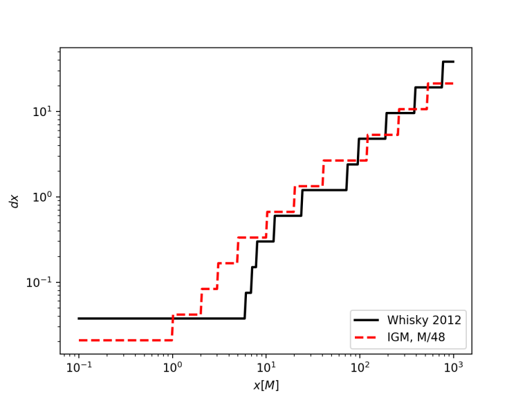
Figure 1: Initial numerical mesh refinement structure for original WhiskyMHD run of Giacomazzo et al. (2012) (black, solid), and lowest-resolution IllinoisGRMHD runs (red, dashed), expressed as local grid spacing $dx$ as a function of “radial distance” $x$ from the puncture at the center of the grid. Both grids have 11 refinement levels, with similar outer resolutions. The IllinoisGRMHD run is better-resolved in the regions immediately around the individual horizons, but the WhiskyMHD run maintained uniformly high resolution for all points within $6M$ of each puncture.

In Fig. 2, we show the resulting Poynting luminosity from both the WhiskyMHD run and the new IllinoisGRMHD run. The peak luminosity is very similar in both cases, but the rise to this peak is sharper in the WhiskyMHD case because under-resolved horizon regions result in a considerably earlier merger time of the black holes in the WhiskyMHD run. We have verified that the different treatment of the polytropic coefficient $\kappa$ between WhiskyMHD and IllinoisGRMHD has minimal effect on the luminosity, by performing a modified IllinoisGRMHD simulation with fixed $\kappa$ (i.e., with shock-heating disabled) (blue curve in Fig. 2).

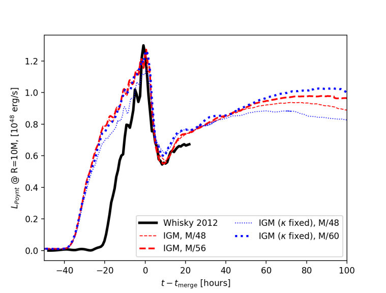
Figure 2: $L_{\rm Poynt}$ for original WhiskyMHD run of Giacomazzo et al. (2012) (black, solid), compared with the new IllinoisGRMHD runs for the same initial separation (red, dashed). All luminosities have been time-shifted by the time of merger for that run, and scaled to reflect the canonical case in Giacomazzo et al. (2012): a plasma of uniform initial density $\rho_{0}=10^{-11}\,{\rm g}\,{\rm cm}^{-3}$ and magnetic field strength $B_{0}=3.363\times 10^{4}\,{\rm G}$, in the vicinity of a black-hole binary of total mass $M=10^{8}M_{\odot}$. An IllinoisGRMHD simulation keeping the polytropic coefficient $\kappa$ fixed to its initial value everywhere (i.e., disabling shock heating) shows very similar behavior (blue, dotted).

IV Results

Our simulations are designed to explore the MHD physics that may give rise to EM counterparts to black hole mergers. These simulations, however, are not appropriate over the large temporal and spatial scales required to simulate the emission of EM radiation to a very distant observer (“at infinity”); the black hole region is fully enshrouded by an infinite region of finite-density gas which would soon block any radiation or other outflows. Our focus instead is to examine near-zone mechanisms that could drive EM outflows. Two broad channels of emission are considered. First, the development of familiar jet-like structures leading to strong Poynting flux on the axis can provide a significant source of energy, which can be converted to strong EM emissions farther downstream. Second, we also consider mechanisms for direct emission from the fluid flows near the black holes, ignoring the absorbing properties of matter farther out.

Our canonical configuration is an equal-mass BBH with initial coordinate separation $d=14.4M$, initial fluid density $\rho_{0}=1$ in a polytrope with $\kappa=0.2,\Gamma=4/3$, and initial magnetic field strength $b_{0}=0.1$. We present these and derived parameters in Table 1.

Table 1: Initial parameters and derived quantities for the canonical configuration: initial puncture separation $d$, puncture mass $m_{\rm p}$, Bowen-York linear momentum components $P_{\rm tang}$ & $P_{\rm rad}$, finest grid spacing $dx$, merger time $t_{\rm merge}$, initial fluid density $\rho_{0}$, magnetic field strength $b_{0}$, polytropic constant $\kappa_{0}$, fluid pressure $p_{0}$, specific internal energy $\epsilon_{0}$, ratio of magnetic to fluid energy density $\zeta_{0}$, specific enthalpy $h^{*}_{0}$, and ambient Alfvén speed $v_{\rm Alf}$.

$d(M)$	$m_{\rm p}$	$P_{\rm tang}(M)$	$P_{\rm rad}(M)$	$dx(M)$
14.384	0.4902240	0.07563734	-0.0002963	1/48

$t_{\rm merge}(M)$	$\rho_{0}$	$b_{0}$	$\kappa_{0}$	$p_{0}$	$\epsilon_{0}$	$\zeta_{0}$	$h^{*}_{0}$	$v_{\rm Alf}$
3514.333	1.0	0.1	0.2	0.2	0.6	5.0e-3	1.81	0.07433

IV.1 Large-Scale Structure of Fluid and Fields

We begin by presenting an overview of the major field structures that develop through MHD dynamics during the merger process, using our canonical case as a representative example.

The canonical simulation begins about $3500M$ before merger, with an initially uniform fluid and a uniform vertical magnetic field. After some time the fluid has fallen mostly vertically along the field lines, concentrating in a nearly axisymmetric thin disk ($h\ll M$) of dense material about each black hole. Figure 3 shows a snapshot of the fluid density $\rho$ on the $x$-$y$ (orbital) and $x$-$z$ planes during the late inspiral (about $1100M$ before merger) for the $d=14.4M$ configuration.

Figure 3: Fluid density $\rho$ during inspiral at time $t=2400M$ (about $1100M$ before merger) for the $d=14.4M$ configuration. At this time the holes are centered at $(x,y)\approx\pm(5.53M,0.08M)$. The regions inside the BH horizons have been masked out. Note that in all configurations the BHs are orbiting in a counter-clockwise motion around the positive $z$ axis

By late times, those disks have merged into a common disk around the final, spinning black hole. The structure of the post-merger disk is shown in Fig. 4, where we again plot $\rho$ on the $x$-$y$ and $x$-$z$ planes. By this time fluid has fallen in to form a thin disk ($h\ll M$) of dense material with radius of $2-3$ gravitational radii (the BH horizon radius is approximately $1M$ here). Above and below the disk, gas is largely excluded by magnetically dominated regions. Focusing just on the $x$-$y$ plane, the top panel shows that some asymmetric structure persists long after merger.

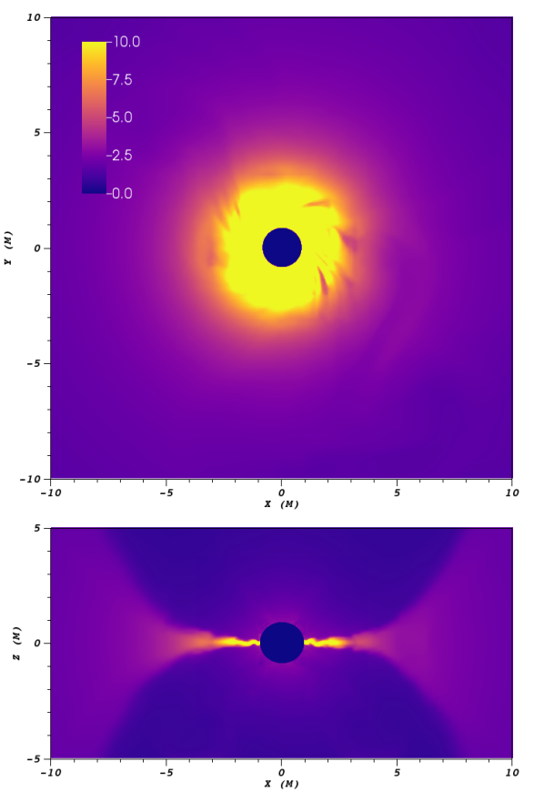
Figure 4: Fluid density $\rho$ approximately $1500M$ after merger for the $d=14.4M$ configuration. The region inside the BH horizon has been masked out.

Though these pre-merger and post-merger disks superficially resemble familiar black hole accretion disks, there are important differences. Traditional disks are centrifugally supported outside the innermost stable circular orbit. Our fluid distribution, on the other hand, is initially at (coordinate) rest with low specific angular momentum. While these flows are stirred first by binary motion and later by frame-dragging near the final spinning black hole, this does not produce a Keplerian flow. This can be seen in Fig. 5, which shows the fluid orbital frequency $\Omega_{\rm fluid}$ (7) about $1100M$ after merger. The region around the horizon exhibits a spin-up of the fluid material for $r\lesssim 4M$ to an angular frequency of up to $M\Omega_{\rm fluid}\sim 0.1$. This can be compared with two other angular velocity profiles of interest: the Keplerian angular velocity $\Omega_{K}$ (8) for a rotationally supported disk, and the “infall angular velocity” (9) for equatorial infall geodesics with vanishing specific angular momentum. Each is evaluated for the same Kerr BH ($a=0.69M$). The velocity profile of our disk more closely resembles the profile of infalling geodesics.

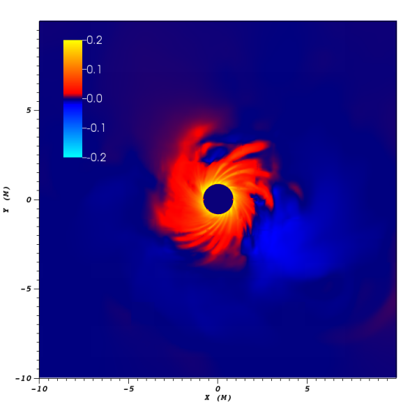
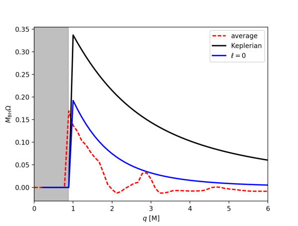
Figure 5: Top panel: Post-merger fluid orbital frequency $\Omega_{\rm fluid}$ for the high-resolution $d=14.4M$ configuration. The black-hole interior has been masked out. Bottom panel: $M_{\rm BH}\Omega_{\rm fluid}$ as function of cylindrical radius $q$, averaged over orbital azimuthal angle (red dashed), with the corresponding relativistic Keplerian angular frequency $M_{\rm BH}\Omega_{K}$ (black solid), and the angular frequency induced for a zero-angular-momentum ($\ell=0$) infalling test particle (blue solid). The shaded region marks the interior of the black-hole horizon.

During evolution, the initially parallel, $z$-directed magnetic field lines evolve to resemble the structure of a black-hole jet. The field lines are pinched in the orbital plane as the matter falls in through the disk region, and become twisted into a helical structure—see Fig. 6—through the rotational motion in the orbital/infall plane. This structure originates in the strong-gravitational-field region and propagates outward at the ambient Alfvén speed $v_{\rm Alf}$ (10).

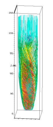
Figure 6: Magnetic field streamlines in the polar region, around $1100M$ after merger. The field lines are twisted into a helical pattern, concentrated at the origin. This helical structure propagates outward at the ambient Alfvén speed $v_{\rm Alf}=0.07433$, replacing the initially vertical $B$ fields (still visible at large $z$).

This process also enhances the magnetic field strength in the region above and below the orbital plane. In Fig. 7, we show the state of the evolved (squared) magnetic field strength $b^{2}$ $1100M$ after merger, evaluated on the $x$-$z$ plane. As seen in the top panel, $b^{2}$ is greatly amplified at and near the polar axis of the post-merger hole. The lower panel shows that this region is dominated by magnetic pressure.

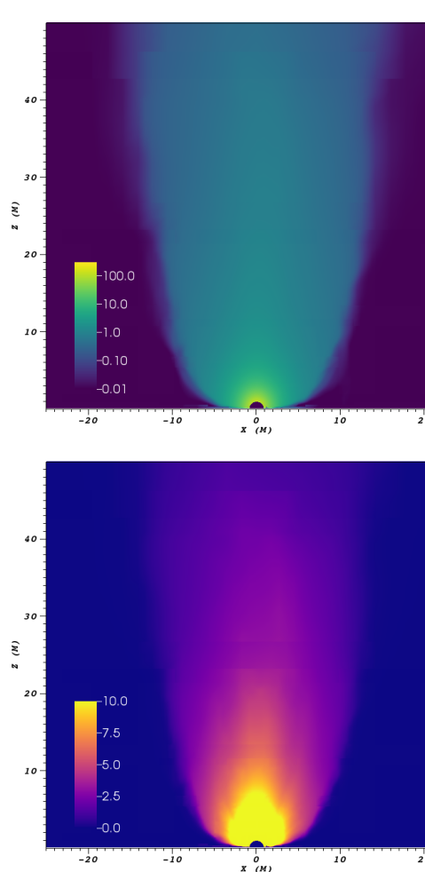
Figure 7: Top panel: Magnetic field squared magnitude $b^{2}$ about $1100M$ after merger for the high-resolution $d=14.4M$ configuration. Bottom panel: Magnetic-to-gas pressure ratio $\beta^{-1}\equiv b^{2}/2p_{\rm gas}$ for the same time and configuration.

This region shares some features of a relativistic jet, as both are magnetically dominated and contain a helical magnetic field structure. We show in Fig. 8 that the structures we observe yield a strong Poynting flux directed outward. As with our disk however, through the course of these simulations the fluid flow through these jet-like structures is predominantly inward-directed. Nonetheless, over longer temporal and larger spatial scales and in plausible astrophysical environments, the strong Poynting flux could drive relativistic outflows and strong EM emissions. We further explore this as a source of energy to eventually power EM counterparts in the next section.

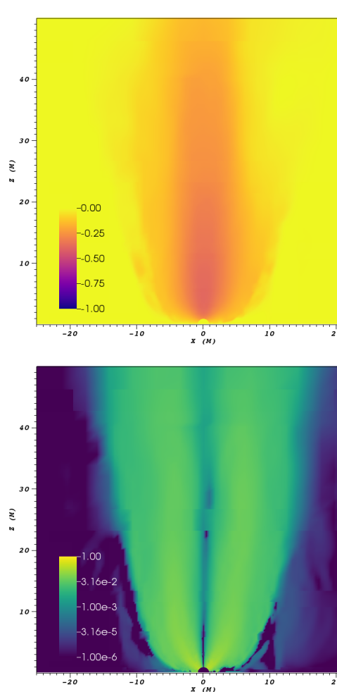
Figure 8: Top panel: Fluid velocity ($z$ component) about $1100M$ after merger for the high-resolution $d=14.4M$ configuration. Bottom panel: Poynting vector (11) ($z$ component) for the same time and configuration.

IV.2 Mass Accretion Rate

Although the initially static fluid in our simulations does not develop the rotational support necessary for an accretion disk (as Fig. 5 indicates), the rate of accretion $\dot{M}$ onto the black holes provides a measure of the energy available for EM outflows during inspiral and merger. In Fig. 9, we show the development of this quantity over the bulk of the $d=14.4M$ evolution, calculated using (13).

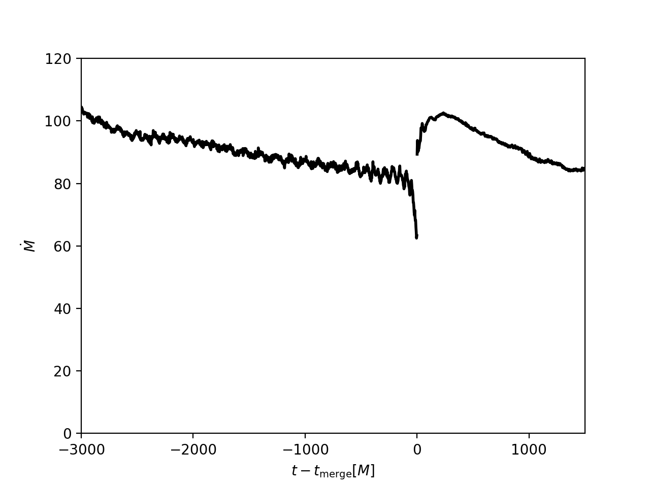
Figure 9: Rate of mass loss $\dot{M}$ to accretion into the black hole horizons.

We note the main features of this accretion rate estimate: (i) $\dot{M}$ slowly declines through the late inspiral, with the drop-off steeper just before merger when a common horizon forms; (ii) $\dot{M}$ jumps when the black hole apparent horizons join discontinuously at merger; (iii) after some settling in, the post-merger $\dot{M}$ resumes the slow decline seen before merger.

The numbers in Fig. 9 are in code units where $M=1$, $\rho_{0}=1$. Since $\dot{M}$ generically scales as $\rho M^{2}$, we convert to physical units using a factor $G^{2}/c^{3}$. Scaling for our canonical initial fluid density and system mass, we obtain the rate in cgs units as

$$\dot{M}_{\rm cgs}=6.54\times 10^{23}{\rho_{\textnormal{-}13}}M_{8}^{2}\dot{M}\,{\rm g}\,{\rm s}^{-1},$$ (14)

where ${\rho_{\textnormal{-}13}}\equiv\rho_{0}/(10^{-13}\,{\rm g}\,{\rm cm}^{-3})$, and $M_{8}\equiv M/(10^{8}M_{\odot})$.

Since $\dot{M}\sim 100$ throughout the simulation, a good order-of-magnitude estimate for the accretion rate both before and after merger is $\dot{M}_{\rm cgs}\approx 6\times 10^{25}{\rho_{\textnormal{-}13}}M_{8}^{2}\,{\rm g}\,{\rm s}^{-1}$.

IV.3 Features of Poynting Luminosity

The powerful Poynting flux generated by our simulations shows that strong flows of electromagnetic energy are driven vertically outward along the orbital angular momentum axis, starting near the orbital plane. Many studies have shown that such Poynting flux regions can transfer power from the black hole region, driving relativistic outflows Blandford and Znajek (1977); Paschalidis et al. (2015); Ruiz et al. (2016), and then through a cascade of internal or external matter interactions, ultimately yielding strong EM emissions (e.g., in the fireball model for gamma-ray bursts Piran (1999)). Our simulations are not set up to model those processes, but we can explore the Poynting luminosity as a potential source of power for EM counterpart signals.

To get a measure of time dependence of the jet-like Poynting-driven EM power, we compute the Poynting luminosity $L_{\rm Poynt}$ from (12), using the dominant $(l,m)=(1,0)$ spherical harmonic mode of the $z$-component of the Poynting flux, $S^{z}$ (11), extracted on a coordinate sphere of radius $R=30M$. Results from this diagnostic are shown in Fig. 10. As discussed in Appendix A, this rotation-axis-aligned component dominates the Poynting flux: $S^{r}\approx S^{z}\cos\theta$. We select extraction at $30M$ as giving a measure of the input energy for potential reprocessing into EM signals down stream. This extraction radius is far enough to avoid confusion with the motion of the black holes, yet close enough to provide a quick measure of potential emission on timescales comparable to the merger-time.

Several features are evident in Fig. 10: (a) an early local maximum in the flux (occurring at $t\sim 100M$ for this extraction radius); (b) a steep rise in flux amplitude beginning at $t\sim 450M$, followed by (c) a slight drop to a slow-growth stage, ending in a rapid climb and with a slight “blip” (d), leading to a final maximum value (e) before a gradual fall-off. We believe that these features correspond to (a) the initial settling of the GRMHD fluids and black hole space-time, (b) the arrival of magnetic-field information from the black hole region at the extraction sphere, (c) development relating to the inspiral process, (d) prompt response to merger, and (e) initiation of single-black hole jet-like characteristics.

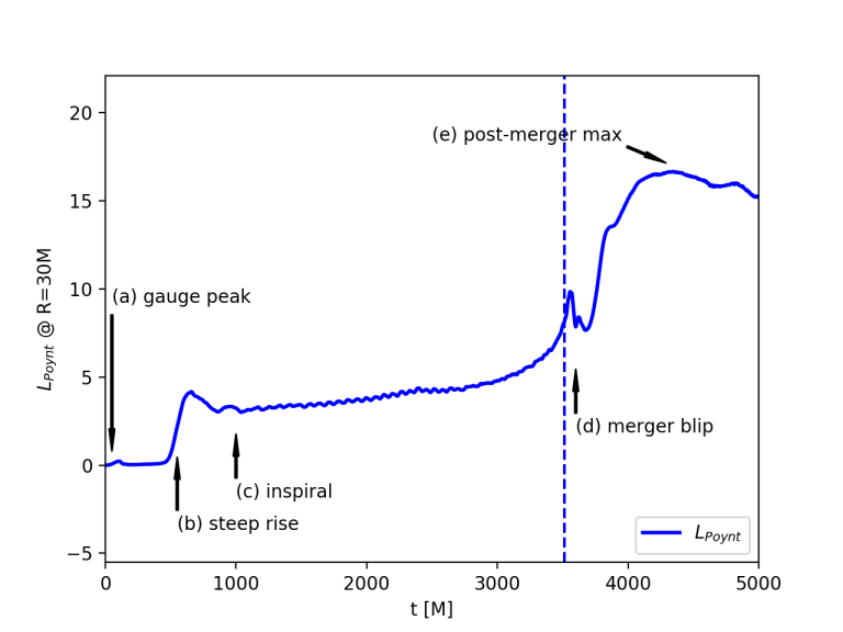
Figure 10: $L_{\rm Poynt}$, the Poynting luminosity, for the $d=14.4M$ configuration considered in Table 3; extraction of the mode is on a coordinate sphere of radius $30M$. The merger time is marked by a dashed vertical line.

IV.3.1 Dependence on Initial Separation

The plasma in our simulations is initially at rest near the black holes, which is clearly unphysical. We must therefore be careful to start our BBH at a large enough separation so that plasma in the strong-field region has time to establish a quasi-equilibrium flow with the binary motion.

Binary parameters for simulations covering a range of initial separations are presented in Table 2. To treat the limit of zero initial separation, we also performed a simulation of a single Kerr black hole (using the quasi-isotropic form of exact Kerr Brandt and Seidel (1996)) with parameters chosen consistent with the end-state black hole observed after merger: $m_{\rm Kerr}=0.97M$, $a/m_{\rm Kerr}=0.69$.

Table 2: Bowen-York parameters of the numerical configurations used. The holes are non-spinning, and are initially separated in the $x$ direction. Our canonical configuration is shown in bold face.

run name	$d(M)$	$m_{\rm p}$	$P_{\rm tang}(M)$	$P_{\rm rad}(M)$
X1_d16.3	16.267	0.4913574	0.07002189	-0.0002001
X1_d14.4	14.384	0.4902240	0.07563734	-0.0002963
X1_d11.5	11.512	0.4877778	0.08740332	-0.0006127
X1_d10.4	10.434	0.4785587	0.0933638	-0.00085
X1_d9.5	9.46	0.4851295	0.099561	-0.001167
X1_d8.4	8.48	0.483383	0.107823	-0.0017175
X1_d6.6	6.61	0.4785587	0.1311875	-0.0052388

Table 3: Time of merger $t_{\rm merge}$ for each binary configuration. As time of merger depends on resolution, we include resolution information for each case. Our canonical configuration is shown in bold face.

run name	$dx(M)$	$t_{\rm merge}(M)$
X1_d16.3	1/48	5380
X1_d14.4	1/48	3514
	1/56	3651
	1/72	3797
X1_d11.5	1/48	1549
	1/56	1584
	1/72	1572
X1_d10.4	1/48	1054
	1/72	1066
X1_d9.5	1/48	681
X1_d8.4	1/48	451
	1/56	451
X1_d6.6	1/48	208

In Fig. 11 we again show $L_{\rm Poynt}$ at $R=30M$, but for simulations beginning at times ranging from about $200M$ to $5400M$ before merger. For convenience, we show the merger time of each configuration as a dashed line of the same color. While we generally see the same set of features for each simulation, the time delay between features (b) and (d) shrinks as the inspiral duration becomes shorter.

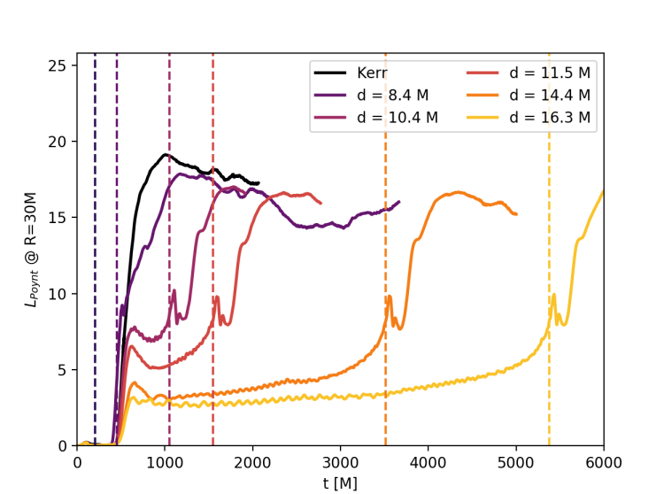
Figure 11: $L_{\rm Poynt}$ for the configurations considered in Table 3; extraction of the mode is on a coordinate sphere of radius $30M$ for each case. Merger times for each binary are marked by dashed vertical lines. ($1L_{\rm Poynt}=5.867\times 10^{44}{\rho_{\textnormal{-}13}}M_{8}^{2}\,{\rm erg}\,{\rm s}^{-1}$.)

The timing of features (a) and (b) indicates that they can have no dependence on the merger of the binary, in contrast to the conclusion drawn from the 2012 work Giacomazzo et al. (2012). For initially smaller-separation simulations such as the $d=8.4M$ of Giacomazzo et al. (2012), these features are poorly resolved; in particular the “slow-growth” stage is almost completely absent. Consequently Giacomazzo et al. (2012) failed to distinguish the initialization-dependent rise (b) from the inspiral- and merger-driven rise (c-e).

The blip (d) and the rise surrounding it do appear to be correlated with the merger time. In Fig. 12, we realign the flux curves of Fig. 11 by merger time $t_{\rm merge}$ (time when a common apparent horizon is first found; see Table 3). It can be seen that the general trend with larger separation has been to reveal a consistent pre-merger portion of the flux. After an initial settling-in, the flux rises slowly as the binary system inspirals.

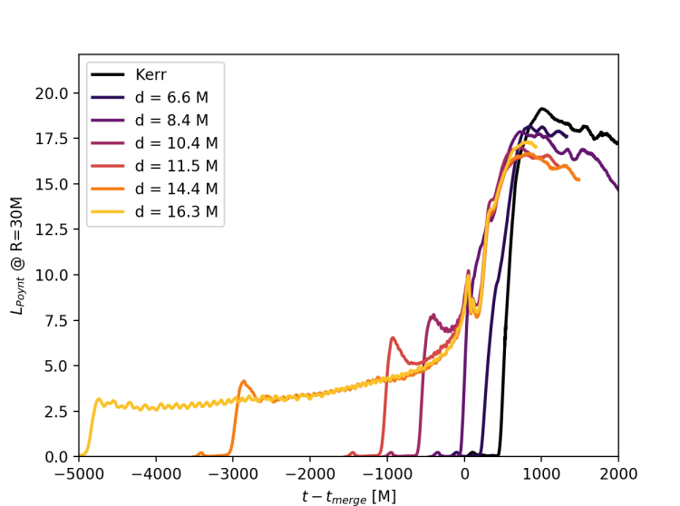
Figure 12: As in Fig. 11, but with time axis aligned by merger time of the binary. ($1L_{\rm Poynt}=5.867\times 10^{44}{\rho_{\textnormal{-}13}}M_{8}^{2}\,{\rm erg}\,{\rm s}^{-1}$.)

In Appendix B we explore the robustness of this result to changes in the extraction radius and to numerical resolution changes. Overall the level and shape of the curve in Fig. 12 provides a picture of the time-dependence of the available jet power, which is robust at roughly the ten-percent level.

IV.3.2 Magnetic Field Dependence of Poynting Luminosity

In the previous subsections we found a “light curve” for the time dependence of outgoing Poynting flux for a canonical ambient fluid density and aligned magnetic field strength of $b_{0}=0.1$. However, it is natural to expect that features of EM flux will change as the initial ambient field strength varies. In previous studies carried out in the force-free limit Neilsen et al. (2011); Palenzuela et al. (2010c) the Poynting flux necessarily scaled with the square of the initial magnetic field strength. On the other hand, if the matter flows play an important role in driving magnetic field development, then we should expect a different scaling.

Here we investigate this issue by looking at several $d=14.4M$ configurations that differ only in their initial uniform magnetic field strength $b_{0}$. The different field parameters are presented in Table 4, along with the resulting Alfvén speeds $v_{\rm Alf}$.

Table 4: Initial uniform GRMHD field values for canonical $d=14.4M$ configuration (b1e-1) (shown in bold face) and variants discussed in Secs. IV.3.2 and IV.3.3.

config	$\rho_{0}$	$b_{0}$	$\kappa_{0}$	$p_{0}$	$\epsilon_{0}$	$\zeta_{0}$	$h^{*}_{0}$	$v_{\rm Alf}$
b1e-1	1.0	0.1	0.2	0.2	0.6	5.0e-3	1.81	0.074
b1e-2	1.0	0.01	0.2	0.2	0.6	5.0e-5	1.8	0.0075
b3e-2	1.0	0.03	0.2	0.2	0.6	4.5e-4	1.8	0.022
b3e-1	1.0	0.3	0.2	0.2	0.6	4.5e-2	1.89	0.22
b1e0	1.0	1.0	0.2	0.2	0.6	5.0e-1	2.8	0.60
b1e-1_up	100.0	1.0	0.0431	20.0	0.6	5.0e-3	1.81	0.074
b1e-1_down	0.01	0.01	0.928	2.0e-3	0.6	5.0e-3	1.81	0.074

Figure 13 shows the resulting Poynting luminosities on a logarithmic scale. While the flux in all cases exhibits a very small early amplification (the “initial-settling” peak (a) in Fig. 10) whose timing is insensitive to field strength, the later rise to levels observed during inspiral is significantly accelerated or retarded relative to our canonical case, with stronger ambient fields rising more quickly. The “rise time” is consistent with a feature traveling outwards at the initial ambient Alfvén speed $v_{\rm Alf}$ (see Table 4), as $v_{\rm Alf}\propto b^{2}$ in non-magnetically dominated regions (Eq. 10).

More surprisingly, however, each configuration appears to reach the same level of Poynting luminosity during inspiral, regardless of initial field strength (only the weakest of the five cases does not share this common inspiral luminosity, presumably because $v_{\rm Alf}$ is too low for the disturbance to reach the observer at $R=30M$ before merger). This is important because insensitivity to details of astrophysical conditions at the time of merger, as we seem to see with magnetic field strength in this case, would be an important factor in any potentially robust electromagnetic signatures of black hole mergers.

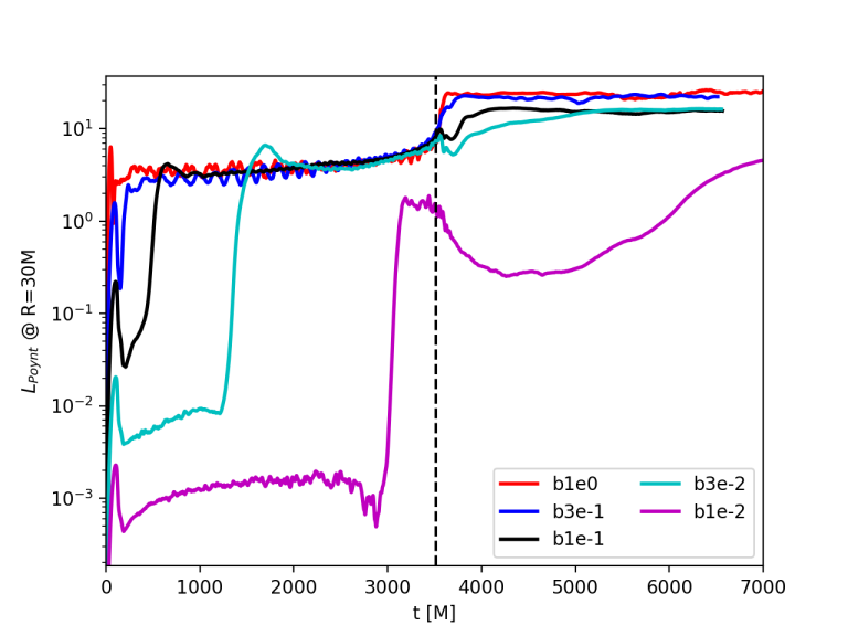
Figure 13: $L_{\rm Poynt}$ for low-resolution $d=14.4M$ configuration, for five different magnetic field strengths $b_{0}$, extracted at $R=30M$. The common merger time is indicated by the dashed vertical line. ($1L_{\rm Poynt}=5.867\times 10^{44}{\rho_{\textnormal{-}13}}M_{8}^{2}\,{\rm erg}\,{\rm s}^{-1}$.)

To understand this apparent universality of the Poynting luminosity during inspiral, we next analyze how the magnetic field is amplified in the vicinity of the binary. In the upper panel of Fig. 14, we show the evolved field $b^{2}$ as extracted along the orbital ($z$) axis for these configurations at time $t=5000M$, about $1500M$ after merger. We see that, while $b^{2}$ asymptotes to its initial value far from the origin, the amplified fields closer in tend to a common level. Indeed, within $\sim 10M$ of the origin, the top four configurations are nearly indistinguishable, reaching a common value of $b^{2}_{\rm max}\approx 100$ (similar to what was reported in Giacomazzo et al. (2012)). The lower panel shows $b^{2}$ measured at the same time, but along a line parallel to the $x$ axis, at a height $z=10M$. As the configuration is highly axially symmetric around the orbital ($z$) axis by this time, this represents the general falloff of $b^{2}$ with distance from the orbital axis. Grouping of the curves in the region $x<10M$ shows that the consistency of $b^{2}$ along the axis is representative of the field strength across most or all of the jet-like region.

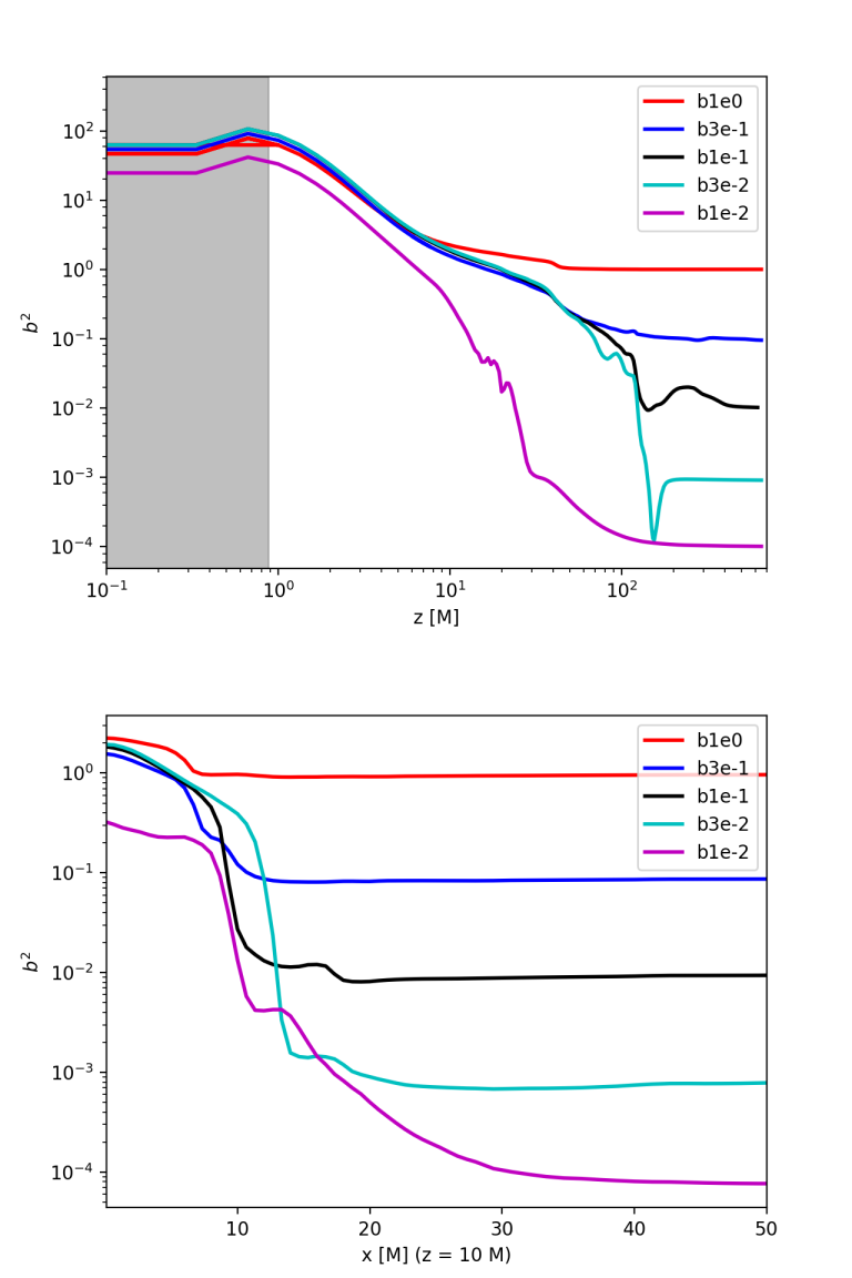
Figure 14: Top panel: Evolved magnetic-field variable $b^{2}$ along the polar ($z$) axis at time $t=5000M$. The shaded region marks the interior of the black-hole horizon. Bottom panel: $b^{2}$ along line parallel to $x$-axis, at $z=10M$.

This common magnetic field magnitude suggests a physical process in which gravitationally driven matter flows drive up the magnetic field to the point of saturation. The saturation likely reflects a point of overall balance between magnetic pressure and gravitationally driven matter pressure. Whatever the mechanism’s details, its effect is that the arbitrary initial fields are replaced by a universal, magnetically dominated helical structure. The outgoing Poynting flux thus also tends to a common level. We remind the reader that our simulations scale with an arbitrary initial gas density $\rho_{0}$. As the density increases, the magnetic field strength should scale with $\rho^{1/2}$.

IV.3.3 Scaling Behavior of Luminosity

In the matter-free simulation of black-hole mergers, the timescale and all observables (e.g. gravitational-wave amplitude and frequency) scale with (or inversely to) the total mass $M$ of the system; thus the same simulation can describe the merger of a stellar-mass system or a supermassive one.

The results of our GRMHD simulations in this work are not so trivially rescaled. In fact, for a given binary mass $M$ (which sets the timescale), the Poynting luminosity scales cleanly only with the combination $\{\rho_{0},p_{0},b_{0}^{2}\}$. That is, if we wish to scale the magnetic field strength $b^{2}_{0}$ by a factor $C$, then the same dynamics applies as long we also scale the initial baryonic density $\rho_{0}$ and the pressure $p_{0}$ by the same factor. The time-dependent Poynting luminosity is then $C$ times the original. We demonstrate in Fig. 15 that this scaling is realized computationally.

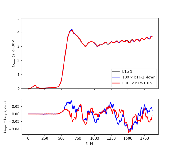
Figure 15: Top panel: $L_{\rm Poynt}$ for low-resolution $d=14.4M$ configuration, for the three different choices of $\{\rho_{0},p_{0},b_{0}^{2}\}$. Bottom panel: difference between the canonical b1e-1 configuration and each of the other two.

This scaling invariance should not be surprising, since the total stress-energy tensor (6a) is homogeneous in these three quantities. As long as gravitational effects from the matter fields are not relevant then the dynamics will be independent of $C$. Consequently all velocities, including for instance the Alfvén velocity (10), are independent of this collective rescaling. If we further write the magnetic-fluid energy density ratio as $\zeta_{0}\equiv b_{0}^{2}/(2\rho_{0})$, then the uniform scaling performed in this section is equivalent to scaling the initial fluid density $\rho_{0}$ while keeping the specific internal energy $\epsilon_{0}$ and the energy-density ratio $\zeta_{0}$ constant.

For a fixed fluid density $\rho$, the luminosity scales with volume divided by time. In geometric units, this ratio scales as $M^{2}$. Thus the luminosity satisfies the scaling relation

$$L_{\rm Poynt}(t)=\rho_{0}M^{2}F(t/M;\epsilon_{0},\zeta_{0}),$$ (15)

where $F(t/M;\epsilon_{0},\zeta_{0})$ is a dimensionless function of time. In the context of EM counterparts this scaling differs from many other emission models that scale roughly with $M$, as in Eddington-limited accretion. Note that our study does not model EM radiation feedback, which would control an Eddington-limited process Krolik (2010).

The choice of initial density, however, can itself be influenced by the total mass of the system. For instance, consider the geometrically thick accretion disks investigated by Gold et al. (2014a), $\rho_{0}\sim M^{-1}$. In such a system, the Poynting luminosity (15) will scale linearly with $M$. Our results above indicate furthermore that $F(t/M;\epsilon_{0},\zeta_{0})$ is effectively independent of $\zeta_{0}$ over a significant range of magnetic field strength. Of course, in the limit of extreme magnetic dominance, we expect the FFE description to apply, where density can be assumed to be irrelevant, and the luminosity scales with magnetic field squared.

At least for the simple class of astrophysical scenarios covered in our simulations we conclude that Poynting flux—as a time-dependent driver for jet energy—is largely independent of several astrophysical details, particularly magnetic field strength, up to a simple scaling. Next we consider the relation of its time dependent behavior to orbital dynamics.

IV.3.4 Relation between Poynting luminosity and Orbital Motion

Several numerical Palenzuela et al. (2010c, b); Neilsen et al. (2011); Paschalidis et al. (2013) and analytical Lyutikov (2011); McWilliams and Levin (2011); Penna (2015); Morozova et al. (2014) studies have investigated how even non-spinning black holes in an orbital configuration can generate Poynting luminosities in the limit of force-free MHD through a process similar to the Blandford-Znajek mechanism Blandford and Znajek (1977) for jets powered by a black hole. In Blandford-Znajek, the twisting of magnetic field lines in interaction with a spinning black hole converts kinetic energy to jet power. Before merger, however, the dragging of black holes through the ambient field similarly converts kinetic energy to jet power. While there are differences in the computed efficiency of this conversion, a general picture emerges that (for nonspinning black holes in the inspiral phase) the Poynting luminosity scales as

$$L_{\rm FFE,insp}\sim v^{2}B^{2}M_{\rm BH}^{2}.$$ (16)

A difference with our simulations is that our black holes do not orbit in a magnetically dominated, force-free environment. Here we investigate whether a similar velocity scaling still holds, analyzing data in the case with the longest inspiral: $d=16.3M$.

We derive instantaneous BH velocity data from the motion of the BH horizons given by our apparent horizon finder. While these velocities are not gauge-invariant, in practice they are reliable after an initial settling-in time of $\sim 50M$ and before the formation of the common horizon at merger.

Complicating this issue is the time lag between the source motion and the resulting Poynting flux present in fields measured farther out. In Fig. 16, we show the best fit between $L_{\rm Poynt}$ as measured at $R=30M$ and the measured speed, assuming $L_{\rm Poynt}(t)=Av^{n}$, where $v$ is measured at time $t$ offset by some fixed time $\Delta$, representing propagation from the strong-field region of the BHs to the extraction radius $R$. The best-fit parameter values are $\Delta=100M$, $A=870$, and $n=2.7$, based on $L_{\rm Poynt}$ over an inspiral “segment” beginning once $L_{\rm Poynt}$ has settled down into the inspiral regime, and ending at the merger blip (times indicated by vertical dashed lines in the Figure).

The best-fit value $\Delta=100M$ is consistent with $L_{\rm Poynt}$ propagating from the strong-field region out to $R=30M$ at an effective speed of $v_{\rm prop}\approx 0.33c$. In principle, if we know that the Poynting flux is always propagating outward at a well-defined Alfvén speed $v_{\rm Alf}$, we can derive the necessary time shift $\Delta$ from that. However, $v_{\rm Alf}$ changes with time and position — increasing as the underlying $b^{2}$ grows and $\rho$ declines — and such a detailed analysis is beyond the scope of this paper.

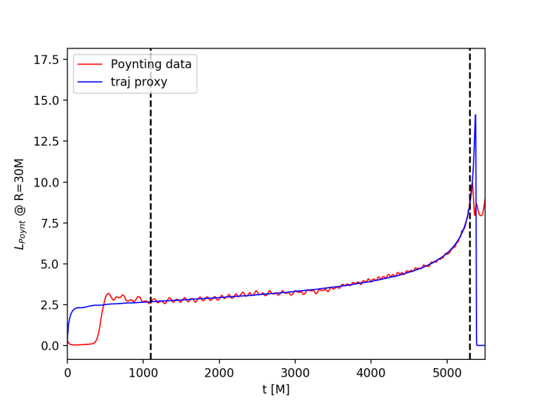
Figure 16: Best scaling of form $Av^{n}$ to match puncture speed $v$ with $L_{\rm Poynt}$ as extracted at $R=30M$. The dashed vertical lines indicate the beginning and end of the fit region.

Thus we can deduce that for a fixed initial field configuration, during the inspiral phase the Poynting luminosity depends on the orbital motion as

$$L_{\rm Poynt,insp}(t)\approx A\rho_{0}M^{2}v^{n}(t_{\rm ret}),$$ (17)

with best-fit values $A=870$, $n=2.7$ and $t_{\rm ret}=t-100M$. While this result is derived from just one of our runs, we have established above that the inspiral portion of our runs yields similar results independent of the magnetic field strength and of the initial orbital separation at which we set the plasma to be at rest in our numerical coordinates. In our case, it is the fluid density that scales the luminosity, and that seems to regulate the magnetic field strength. Independent of the observed invariance to initial magnetic field strength, comparison with (16) reveals an enhanced brightening as the velocity increases. One interpretation of this enhancement would be that a mechanism similar to that observed in the FFE studies is also generating power in our studies. However, in our cases the magnetic field strength grows on approach to merger, due to the accretion of gas and thus piling up of field lines near the horizon.

IV.3.5 Formula for Luminosity in Magnetized Plasma

Armed with the observations of the previous subsections, we can summarize our results for Poynting luminosity of the binary at a representative reference point in its “inspiral” phase, and at peak. Given that the BH orbital speed increases only gradually even late in the inspiral, we choose a representative speed $v_{\rm insp}=0.13c$ (this corresponds to a puncture separation of $d\approx 12.2M$, about $2000M$ before merger.). Then from (17), we obtain for the inspiral

$$L_{\rm Poynt,insp} \approx 3.55\,\rho_{0}\,M^{2}$$

$$=3.55\,\eta_{\rm cgs}\,{\rho_{\textnormal{-}13}}\,M_{8}^{2}\,{\rm erg}\,{\rm s}^{-1}$$

$$\approx 2.1\times 10^{45}\,{\rho_{\textnormal{-}13}}\,M_{8}^{2}\,{\rm erg}\,{\rm s}^{-1},$$ (18)

where we use the conversion factor $\eta_{\rm cgs}$ from Eq. (35) to convert from code units to cgs.

Judging from Fig. 12, the post-merger peak of $L_{\rm Poynt}$ is around $17$ in code units for our canonical case. However, this is derived from a set of simulations carried out at modest resolution ($M/48$). As noted in Appendix B, post-merger values of $L_{\rm Poynt}$ increase somewhat with resolution. If we round up so that the peak Poynting luminosity is $L_{\rm Poynt,peak}\approx 20$ in code units, we find

$$L_{\rm Poynt,peak} \approx 20\,\rho_{0}\,M^{2}$$

$$\approx 1.2\times 10^{46}\,{\rho_{\textnormal{-}13}}\,M_{8}^{2}\,{\rm erg}\,{\rm s}^{-1}.$$ (19)

This can be combined with the mass accretion rate found in Sec. IV.2 to estimate a Poynting radiative efficiency around the merger:

$$\epsilon_{\rm EM}\equiv\frac{L_{\rm Poynt,peak}}{\dot{M}c^{2}}\approx 0.22.$$ (20)

IV.3.6 Comparison with Previous Results

In the previous subsection we quantified potential Poynting-flux-powered emissions, synthesizing the results obtained from our GRMHD simulations of mergers with initially non-magnetically-dominated plasmas. We can compare these with the results of previous GRFFE studies Neilsen et al. (2011); Palenzuela et al. (2010b, c) and with previous GRMHD studies of mergers in circumbinary disk configurations Gold et al. (2014a, b); Farris et al. (2012).

Quantitative comparisons depend on assumptions about the astrophysical environment. Leaving aside details of the matter distribution, the environment of our simulations is characterized by a scalable initial gas density relative to a reference density of ${\rho_{\textnormal{-}13}}=1=\rho_{0}/(10^{-13}\,{\rm g}\,{\rm cm}^{-3})$ with an initially uniform poloidal magnetic field. In these units the magnetic field strength of our canonical configuration was $B_{4}=B/(10^{4}\,{\rm G})=0.34{\rho_{\textnormal{-}13}}^{1/2}$, but we found that the Poynting flux is minimally changed if the magnetic field strength is varied by an order of magnitude either up or down. Thus for fixed black hole mass, our overall result for $L_{\rm Poynt}$ simply depends linearly on initial density.

Our study resembles previous GRFFE simulations in that both assume an initially uniform large-scale poloidal magnetic field. As we have noted, the magnetic field structures and the velocity dependence on approach to merger strongly resemble GRFFE results. However, GRFFE results apply in the regime where the fluid is magnetically dominated and are thus independent of density. Instead, the relevant scale parameter for the environment is the magnetic-field energy density. Those authors suppose an astrophysically motivated reference scaling of $B=10^{4}G$. Despite the scaling differences, we can nonetheless compare with our results at particular magnetic-field and fluid density values.

Since the previous GRFFE simulations involved only relatively brief simulations, it makes more sense to compare peak levels of Poynting luminosity. In the figures and discussion of Refs. Neilsen et al. (2011); Palenzuela et al. (2010b, c) the Poynting luminosity tends to rise to a brief peak and then to quickly fall off to a level appropriate for the final spinning black hole, while our luminosities stabilize closer to their peak levels at late times. Taking this and differences in the various FFE papers into account we estimate a peak level from these publications, which can be compared to our Eq. (19), of

$$L_{\rm FFE,peak}\approx 3\times 10^{43}{B_{4}}^{2}\,{M_{8}}^{2}\,{\rm erg}\,{\rm s}^{-1},$$ (21)

reliable within a factor of two. At nominal values the previous GRFFE studies yield a peak Poynting luminosity level about $400$ times smaller than our nominal result, but the assumptions about the astrophysical environments are not quite consistent; in our simulations, the environment is not initially magnetically dominated.

Using the above estimates and expressions, can we then find the value of $B_{4}$ for the GRFFE environment in Eq. (21) to achieve the same Poynting luminosity that we see in our canonical case? The answer is $B_{*4}\approx 20$ plus or minus $50\%$. Converting to the units of our simulations using Eq. 33 for the relevant case ${\rho_{\textnormal{-}13}}=1$, this corresponds to $\zeta=b_{*}^{2}/(2\rho_{0})\approx 18$, which, appropriately enough, is higher than the initial magnetic field strengths of any of our simulations.

We note that the equivalent value $b_{*}^{2}\approx 35$ is close to the evolved $b^{2}$ values seen near the post-merger black hole in our simulations (which we found to be roughly independent of initial field strength; see Fig. 14 and discussion in Sec. IV.3.2).

This suggests the following shorthand description of the comparison between the results of our simulations and previous GRFFE results: The expression (21) for the GRFFE Poynting luminosity gives an approximately correct description of the our initially matter-dominated GRMHD simulations if, in place of the initial magnetic field strength $B_{4}$, the dynamically driven magnetic field strength found near where the jet meets the horizon is used instead.

We can also compare with Poynting luminosities from previous binary black hole simulations with matter initially structured in a circumbinary disk. Using the code on which IllinoisGRMHD is based, Refs. Gold et al. (2014a, b) bring a $\Gamma=4/3$, non-self-gravitating circumbinary disk with a poloidal magnetic field to quasi-equilibrium by allowing an equal-mass BBH to orbit at fixed separation for $\sim$ 45 orbital periods. To ensure quasi-equilibrium could be established with reasonable computational cost, the disk was assumed to be thick ($H/R\sim 0.3$) so that the MHD turbulence (magneto-rotational instability) driving the accretion could be adequately resolved. Beginning from a point about $700M$ before merger, the binary was then allowed to inspiral and merge, solving the full set of general relativistic field equations for the gravitational fields and the equations of GRMHD for the (non-self-gravitating) disk dynamics.

A quantitative comparison of our results with results of Refs. Gold et al. (2014a, b) for circumbinary disks is challenging. First, we can only compare with their fixed choice of magnetic field configuration. Given that we observe some degree of insensitivity to the initial magnetic fields chosen, we will suppose that their field is within a broadly comparable range, noting that their simulations also include regions of gas and magnetic pressure dominance. More fundamental are the density scales near the horizons that power Poynting luminosity. While such densities in our simulations span roughly an order of magnitude, densities in the circumbinary disk simulations span many more. Thus there is no clear way to define a common density as a point of reference for the two studies. Instead, we make a comparison of Poynting luminosities normalized by the mass accretion rate (i.e., “Poynting luminosity efficiency”) during and after merger as an indicator of the supply of gas in the vicinity of the black holes.

The mass accretion rate in Ref. Gold et al. (2014b) varies significantly before merger, but settles to a value near $0.1$ in their units (see their Fig. 3). Scaled by this value, their Poynting luminosity efficiency is close to $\epsilon_{\rm EM}\equiv L_{\rm Poynt}/\dot{M}\approx 0.01$ near merger, growing by about a factor of 5 during the subsequent period of $1000M$. Their peak efficiency is reached at a similar time after merger as in our simulations, but remains smaller than our peak value (Eq. (20)) by a factor of a few.

IV.4 Simulating Direct Emission from Merger

To this point, we have focused primarily on the Poynting flux as a proxy for EM power from the merging black holes. However, Poynting flux alone is not directly observable; we interpret it as a power source for EM emissions downstream along the jet. An alternative mechanism for EM emissions is direct emission from the plasma fluid.

In our simulations the lack of a realistic equation of state or of any radiative cooling mechanism for the gas makes it difficult to produce a reliable prediction for the actual EM emission. Further, our initial conditions of uniform density and magnetic fields do not capture astrophysical details of the full system that may also contribute to EM emission.

We have carried out a simplified calculation of the EM luminosity generated during the inspiral and merger simulation. To do so, we have used a new version of the Monte Carlo radiation transport code Pandurata Schnittman and Krolik (2013), revised to allow for arbitrary spacetime metrics. While the IllinoisGRMHD simulations generate a real dynamic spacetime by solving Einstein’s equations numerically, for this toy emission model we employ a simplified version of the metric that can be calculated efficiently by Pandurata as a post-processor of the MHD data. As described in Schnittman et al. (2017), the binary four-metric can be instantaneously described by a three-metric $\gamma_{ij}$, lapse $\alpha$, and shift $\beta^{i}$, according to:

$$g_{\mu\nu}=\begin{pmatrix}-\alpha^{2}+\beta^{2}&\beta_{j}\\ \beta_{i}&\gamma_{ij}\\ \end{pmatrix}\,.$$ (22)

Following Campanelli et al. (2006c), we use $\alpha=2/(1+\psi^{4})$, $\beta_{j}=0$, and $\gamma_{ij}=\delta_{ij}\psi^{4}$. The conformal factor $\psi$ is given by

$$\psi=1+\frac{m_{1}}{2r_{1}}+\frac{m_{2}}{2r_{2}}\,,$$ (23)

with $r_{1}$ and $r_{2}$ being the simple Cartesian distances between the spatial coordinate and the primary/secondary masses. For the Christoffel-symbol components $\Gamma^{\rho}_{\mu\nu}$ we take the spatial and temporal metric derivatives analytically based on the puncture trajectories calculated by the apparent horizon finder used in our GRMHD simulations. One advantage of using this simplified metric is that we can easily calculate the photon trajectories “on the fly” and thus do not need to rely on the fast light approximation used by many ray-tracing codes.

Even though Pandurata uses a slightly different metric than that of the GRMHD simulations, the qualitative properties of the spacetime are expected to be very similar. We can avoid some potential numerical problems by normalizing the IllinoisGRMHD fluid 4-velocity everywhere by using the coordinate 3-velocity from IllinoisGRMHD and then using the analytic metric to solve for $u^{t}$ via $g_{\mu\nu}u^{\mu}u^{\nu}=-1$.

Given the fluid velocity at each point and for each data snapshot, a local tetrad can be constructed as in Schnittman and Krolik (2013), from which photon packets are launched and then propagated forward in time until they reach a distant observer or are captured by one of the black holes. Those that reach the observer are combined to make images, light curves, and potentially spectra. We ignore scattering or absorption in the gas, so that all photon packets travel along geodesic paths.

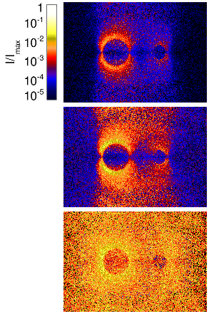
Figure 17: Snapshots from Pandurata post-processing of the simulation data at a separation of $10M$ (about $1000M$ before merger), viewed by an observer edge-on to the orbital plane. Top panel: thermal synchrotron emission; middle panel: magnetic contribution only ($\propto B^{2}$); bottom panel: gas contribution only ($\propto\rho T$).

One of the challenges with this approach is the inherent uncertainty of what emission mechanism is most appropriate, and even then, the electron temperature $T_{e}$ is not known explicitly from the simulations, so it can only be approximated with an educated guess. For this paper, we focused on a single simplified emission model of thermal synchrotron, where the emissivity is isotropic in the local fluid frame with bolometric power density given by

$$P_{\rm syn}=\frac{4}{9}nr_{0}^{2}c\beta^{2}\gamma^{2}B^{2},$$ (24)

with $r_{0}$ the classical electron radius, $n$ the electron number density, $\beta\equiv v/c$, and $\beta^{2}\gamma^{2}\approx T_{e}/m_{e}$ (see, e.g. Chap. 6 of Rybicki and Lightman (1979)). We use the magnetic field strength and fluid density specified by IllinoisGRMHD, along with the code-to-cgs conversion described above. We estimate the electron temperature from the simulation pressure, assuming a radiation-dominated fluid with $p=aT_{e}^{4}$, reasonable for the $\Gamma=4/3$ polytrope used here. Thus the synchrotron power scales as

$$P_{\rm syn}\propto B^{2}\rho^{4/3}\propto\rho_{0}^{7/3},$$ (25)

since $B^{2}\sim\rho$.

In the top panel of Fig. 17 we show the observed synchrotron intensity on a log scale for a single snapshot of IllinoisGRMHD data when the binary separation is $10M$. The observer is located edge-on to the orbital plane and the black hole on the left is moving towards the observer, resulting in a special relativistic boost.

In an attempt to understand the features seen in Fig. 17, we repeat the Pandurata calculations with two other emissivity models, in one case focusing just on the contribution from the magnetic field, and in the other case on the electron density and temperature. As can be seen in Fig. 3, the gas forms two very small, thin disks with magnetically dominated cavities above and below each black hole. From this picture alone, it is not clear where most of the synchrotron flux might originate.

However, when comparing the three panels of Fig. 17, we see that the gas contribution is almost uniformly distributed, and even the thin disks evident in Fig. 3 are almost indiscernible when all the relativistic ray-tracing is included. The reason for this is two-fold. First, the disks are quite small in extent, and the gas is moving almost entirely radially, so the emitted flux is beamed into the horizon, and thus the disks themselves are not clearly visible in the ray-traced image. Second, the overdensity of gas in the disks is only a factor of a few or at most ten greater than the background density. On the other hand, in the funnel regions, $B^{2}$ can be more than four orders of magnitude greater than the ambient or initial pressure, yielding much more significant spatial variations. Thus the synchrotron image (top panel) most closely traces the magnetic field, with a slight enhancement of emission where the gas density and temperature rise near the black holes.

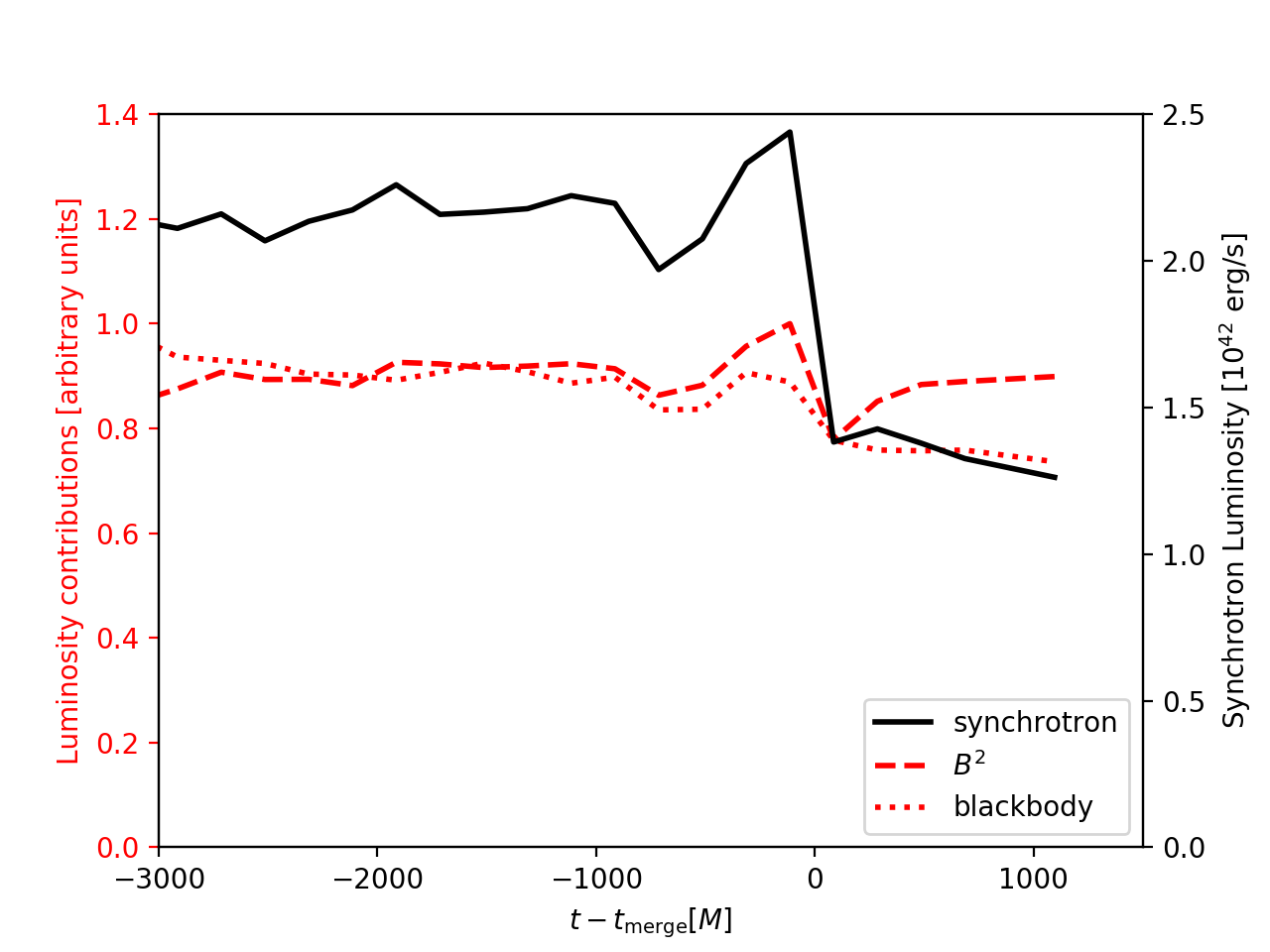
Figure 18: Bolometric luminosity generated in the region $r<30M$ for the X1_d14.4 configuration, assuming the canonical initial density $\rho_{0}=10^{-13}\,{\rm g}\,{\rm cm}^{-3}$. We model local synchrotron emissivity, also showing the development of two contributing components as described in the text.

In Fig. 18 we show the light curve generated by synchrotron emission along with analogous traces computed from the density and magnetic-field components for the X1_d14.4 configuration. To calculate these curves, millions of photons must be launched at each time step, so for efficiency’s sake, we use a relatively coarse time sampling of $200M$. We only consider emission from inside $r<30M$, consistent with the Poynting flux extraction radius.

Figure 18 shows that, unlike the Poynting flux, the locally generated EM power is nearly constant throughout the inspiral leading up to merger. There is a small burst of luminosity preceding merger, followed by a dip of almost $50\%$ for the synchrotron light curve, but the other models show almost no discernible sign of the merger at all. The dip is caused by the sudden expansion of the horizon volume at merger, rapidly capturing the gas with the highest temperature and magnetic field.

Another curious result of the Pandurata calculation is that, for a single snapshot, there is very little difference in the flux seen by observers at different inclination angles or azimuth (of order $\sim 10\%$), suggesting that variability in the EM light curves on the orbital time scale will be minimal.

In principle, Pandurata can also be applied to study the spectra of EM emissions including effects, such as inverse-Compton scattering as photons interact with hot atmospheric plasma, that have been found to be important in modeling black hole accretion disk spectra Schnittman et al. (2013). Our present simulations, however, do not provide a realistic treatment of atmospheric densities and temperatures. Future studies with more detailed physics may reveal more interesting time development in spectral features of the emission.

The above simplifications and caveats mean that we cannot make robust statements about the observability of direct emission. However, based on our optically thin synchrotron emission model, the direct emission luminosity is orders of magnitude lower than that of the Poynting flux. In addition, the synchrotron flux is roughly isotropic, while significant beaming is observed in Poynting flux. There is no contradiction in these measures; Poynting luminosity may manifest as photons far downstream from the GRMHD flows, whereas these direct emission estimates originate in regions of high fluid density and magnetic field strength in strong-gravitational-field zones.

When comparing these direct emissions with results from circumbinary disk simulations, the most similar simulation is in Gold et al. (2014a, b). They estimated a form of direct emission, derived from a cooling function based on hydrodynamic shock heating. The implied cooling luminosity was more than an order of magnitude larger than the Poynting luminosity, while our results suggest that Poynting luminosity is larger than direct synchrotron emission, at least for the canonical density of $10^{-13}\,{\rm g}\,{\rm cm}^{-3}$. We have not incorporated a similar cooling function for a more direct comparison, though we note that our gas does not exhibit strong shocks.

V Conclusions and Future Work

To deepen our understanding of the interplay of gravity, matter, and electromagnetic forces in the vicinity of a merging comparable-mass black-hole binary, we have carried out a suite of equal-mass non-spinning BBH merger simulations in uniform plasma environments. We considered two classes of potential drivers for electromagnetic emissions, primarily focusing on the development of Poynting flux, which may drive a jet, but also considering direct emissions from the fluid.

We conducted simulations covering a range of nearly uniform density, low-velocity distributions of hot gas with a significant but not dominant poloidal magnetic field. Based on these we find that the Poynting luminosity grows on approach to merger (roughly with a power of orbital velocity $v^{2.7}$), leveling off at a steady value after merger. The level and time development of the Poynting luminosity is largely independent of the initial magnetic field strength and not strongly dependent on initial pressure or small changes in fluid configuration, scaling overall with density and the square of black hole mass. Consistent with this we find that the central magnetic field strength is largely independent of the initial field strength, regulated by the gas flow. We further find that the coalescence yields a Poynting efficiency of 0.04 – 0.22 between late inspiral and merger.

These findings, using the new IllinoisGRMHD code, both confirm and extend our earlier GRMHD results obtained with the WhiskyMHD code Giacomazzo et al. (2012), and form a bridge to complementary results from GRFFE codes, in which the plasma is assumed completely magnetically dominated.

Overall consideration of our results with those of previous GRFFE studies suggests a consistent picture where below a transition point near ${B_{4}}^{2}\sim 400{\rho_{\textnormal{-}13}}$, the gas flow dominates and peak Poynting flux is described by our expression (19). Beyond this point the plasma is magnetically dominated and the GRFFE results, summarized in (21) should apply.

To complement Poynting luminosity investigations, we also consider direct synchrotron emission from the plasma in the strong-gravity region near the black holes. To explore the time-dependent bolometric luminosity in this scenario, we employ a new version of the Pandurata code to propagate photons through the IllinoisGRMHD-generated MHD fluids (in post-processing) and generate time-dependent EM flux. Contrary to the Poynting flux analysis we do not find growth in the synchrotron emission on approach to merger. Instead, the luminosity remains steady until it drops to a slightly lower level after merger. Note however that the physical processes behind the two emission mechanisms are mostly independent. Poynting luminosity is due to the highly twisted and amplified magnetic fields in the larger funnel region around the orbital axis, and is expected to accelerate charged particles to produce jet-like behavior leading to EM emission farther downstream; while the direct emission considered here is due to the plasma itself in the more immediate vicinity of the black holes, both before and after merger.

These results provide clues about the physical processes which may drive electromagnetic counterparts to massive black hole mergers, which future GW instruments such as LISA may observe. However limitations to these studies prevent more definitive counterpart predictions. As with many similar studies, our study assumes a large-scale orbit-aligned magnetic field that might approximate the local astrophysical environment near a massive BBH. While some of our results are independent of the level of this field, it provides an asymptotic field structure that we have not strongly justified.

Similarly, while we find that EM emissions are sensitive to ambient gas density, it is unclear how well our very simplified gas distribution, lacking angular momentum support, stands in for real flows from a larger available gas reservoir, such as a circumbinary disk. Our simulations also lack dynamical effects from radiation flows including radiative cooling effects. These limitations will motivate our future work. With more realistic gas distributions in place, we will also investigate the effects of less symmetrical BH systems, including merger recoils Zanotti et al. (2010).

Appendix A Relation of $S^{z}_{(1,0)}$ to Electromagnetic Flux

The quantity $S^{z}_{(1,0)}$ used in the main text is closely related to the EM luminosity calculated by Neilsen et al. (2011); Palenzuela et al. (2010c) in terms of the “outgoing” Newman-Penrose Newman and Penrose (1962) EM radiation scalar $\Phi_{2}=F_{ab}n^{a}\bar{m}^{b}$

$$L_{\rm Poynt}=\frac{dE_{\rm EM}}{dt}=\lim_{R\rightarrow\infty}\oint\frac{R^{2}}{2\pi}|\Phi_{2}|^{2}d\Omega.$$ (26)

The modulus squared of the radiation scalar, $|\Phi_{2}|^{2}$, is proportional to the radial component of the Poynting vector, $S^{R}$. Specifically, if we assume that $\Phi_{2}$ is calculated using the Kinnersley tetrad on a Kerr background, from Teukolsky (1972),

$$T^{r}_{{\rm EM}0}=\frac{1}{2\pi}|\Phi_{2}|^{2}=\frac{1}{\alpha}S^{r},$$ (27)

where the Boyer-Lindquist coordinate (areal) radius $r$ is adopted. As $r$ converges to the numerical radial coordinate at large distances, and the lapse function $\alpha\rightarrow 1$, we see that this is consistent with our definition of $L_{\rm Poynt}$:

$$L_{\rm Poynt}\equiv\lim_{R\rightarrow\infty}\oint R^{2}S^{R}d\Omega$$ (28)

In this case, we can relate the EM flux to the dominant $(\ell,m)=(1,0)$ spherical harmonic mode of the Poynting vector used in this paper via

$$L_{\rm Poynt} =\lim_{R\rightarrow\infty}\oint R^{2}S^{R}d\Omega=\lim_{R\rightarrow\infty}2R^{2}\sqrt{\pi}S^{R}_{(0,0)}$$ (29)

$$\approx\lim_{R\rightarrow\infty}\oint R^{2}S^{z}\cos\theta d\Omega=\lim_{R\rightarrow\infty}2R^{2}\sqrt{\frac{\pi}{3}}S^{z}_{(1,0)}.$$ (30)

This is the formula (12) used in our analysis. In moving from (29) to (30), we have assumed the Poynting flux is dominated by emission along the polar ($z$) direction:

$$S^{R}\approx S^{z}\cos\theta\Rightarrow S^{R}_{(0,0)}\approx\frac{S^{z}_{(1,0)}}{\sqrt{3}}.$$ (31)

This assumption is well-justified for the main part of the flux in the simulations presented here. For example, in Fig. 19, we plot both $S^{z}_{(1,0)}$ and $\sqrt{3}S^{R}_{(0,0)}$ for the $d=14.4M$ configuration. The two signals differ in the initial gauge relaxation pulse (which is therefore not $z$-dominated), but agree closely for the bulk of the signal beginning at $t\sim 500M$.

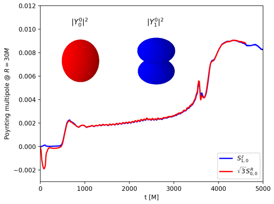
Figure 19: $S^{z}_{(1,0)}$ and $\sqrt{3}S^{R}_{(0,0)}$ extracted at $R=30M$ for the $d=14.4M$ configuration. The two quantities differ in the initial gauge relaxation pulse, but agree closely for the bulk of the signal beginning at $t\sim 450M$, indicating that by this time the approximation $S^{R}\approx S^{z}\cos\theta$ holds.

Appendix B Resolution Tests and Convergence

In Fig. 20, we look at the effect of resolution on the measured EM flux in several of our configurations. It is evident that the general shape of the Poynting luminosity curve near feature (d) is robust to changes in resolution, despite some sensitivity in the quantitative level of the early rise and the post-merger plateau as measured at this extraction radius.

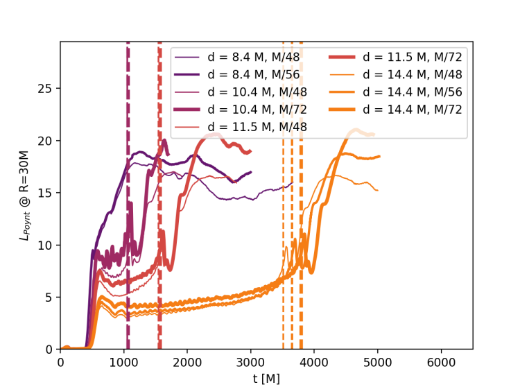
Figure 20: $L_{\rm Poynt}$ for several configurations at basic ($dx=M/48$) and higher resolutions (denoted by thicker lines of the same color).

In Fig. 21, we concentrate on one of the physical cases, $d=14.4M$, and show $L_{\rm Poynt}$ calculated across several extraction spheres, $R/M\in\{30,40,50,60,70,80\}$. We time-shift the different data sets using the initial ambient Alfvén speed $v_{\rm Alf}=0.07433$, which serves to align the initial rise in Poynting flux to the inspiral level. Note that for the least-resolved case ($h_{\rm f}=M/48$), the measured luminosity drops with increased extraction radius $R$; while some dissipation of Poynting flux is possible, the lower panel shows that most of the effect vanishes for higher resolution ($h_{\rm f}=M/72$), pointing to numerical dissipation as a major cause. The shape of feature (d) does vary with the extraction radius, softening as the extraction radius increases.

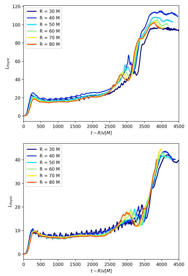
Figure 21: $L_{\rm Poynt}$ for $d=14.4M$ configuration, extracted at different radii, shifted in time consistent with a pulse speed $v=0.07433c$. The lower-resolution run (top) requires an additional multiplicative correction of $R^{n}$ where $n\approx 0.5$ for good alignment, while $n\approx 0.2$ is sufficient for the higher resolution.

Appendix C Converting from Geometric to Gaussian/CGS Units

The initial plasma configuration for the canonical field case was chosen so that $\rho/(b^{2}/2)=200$ far from the strong-field regions. Given that $\rho$ is a matter density, there has to be some conversion for this to make sense.

In Gaussian units, the fluid and magnetic energy densities are

$$u_{\rm fluid}=\rho c^{2},\;u_{\rm magnetic}=\frac{B^{2}}{8\pi}=\frac{b^{2}}{2}.$$

Thus the ratio of the two is

$$\zeta\equiv\frac{u_{\rm magnetic}}{u_{\rm fluid}}=\frac{B^{2}}{8\pi\rho c^{2}}.$$ (32)

Then to get the field strength $B$ given a specified fluid density $\rho$ and energy ratio $\zeta$,

$$B^{2} =8\pi\rho c^{2}\zeta$$

$$=720\pi\times 10^{6}\zeta{\rho_{\textnormal{-}13}}\,{\rm g}\,{\rm cm}^{-1}\,{\rm s}^{-2}$$

$$\Rightarrow B =\sqrt{\frac{36\pi}{5}{\rho_{\textnormal{-}13}}\zeta}\times 10^{4}\,{\rm G},$$ (33)

where we define ${\rho_{\textnormal{-}13}}\equiv\rho/(10^{-13}\,{\rm g}\,{\rm cm}^{-3})$.

Note that the expression (15) is in standard geometric code units, where $G=c=1$. To convert to dimensionful units, we must multiply by a factor $G^{2}/c$. Expressing $\rho_{0}$ and $M$ in cgs units, this factor is approximately $1.483\times 10^{-25}\,{\rm g}^{-2}\,{\rm cm}^{4}\,{\rm s}^{-2}$. That is, we can rewrite (15) as

$$L_{\rm Poynt}(t)=1.483 \times 10^{-25}\left(\frac{\rho_{0}}{1\,{\rm g}\,{\rm cm}^{-3}}\right)\left(\frac{M}{1\,{\rm g}}\right)^{2}$$

$$\times F(t;\epsilon_{0},\zeta_{0}){\rm erg}\,{\rm s}^{-1}.$$

If instead, we scale with our canonical density $\rho_{0}=10^{-13}\,{\rm g}\,{\rm cm}^{-3}$, and a total system mass of $M=10^{8}M_{\odot}=1.989\times 10^{41}\,{\rm g}$, we find

$$L_{\rm Poynt}(t)=5.867\times 10^{44}{\rho_{\textnormal{-}13}}M_{8}^{2}F(t;\epsilon_{0},\zeta_{0})\,{\rm erg}\,{\rm s}^{-1},$$ (34)

where we define ${\rho_{\textnormal{-}13}}\equiv\rho_{0}/(10^{-13}\,{\rm g}\,{\rm cm}^{-3})$ and $M_{8}\equiv M/10^{8}M_{\odot}$. As shorthand, we call this numerical factor $\eta_{\rm cgs}$:

$$\eta_{\rm cgs}\equiv 5.867\times 10^{44}{\rho_{\textnormal{-}13}}M_{8}^{2}.$$ (35)

References

- Abbott et al. (2016a) B. P. Abbott et al. (LIGO Scientific), Phys. Rev. Lett. 116, 061102 (2016a), eprint arXiv:1602.03837 [gr-qc].
- Abbott et al. (2016b) B. P. Abbott et al. (LIGO Scientific), Phys. Rev. Lett. 116, 241103 (2016b), eprint arXiv:1606.04855 [gr-qc].
- Connaughton et al. (2016) V. Connaughton, E. Burns, A. Goldstein, L. Blackburn, et al., Astrophys. J. 826, L6 (2016), eprint arXiv:1602.03920 [astro-ph.HE].
- Perna et al. (2016) R. Perna, D. Lazzati, and B. Giacomazzo, Astrophys. J. 821, L18 (2016), eprint arXiv:1602.05140 [astro-ph.HE].
- Li et al. (2016) X. Li, F.-W. Zhang, Q. Yuan, Z.-P. Jin, Y.-Z. Fan, S.-M. Liu, and D.-M. Wei, Astrophys. J. 827, L16 (2016), eprint arXiv:1602.04460 [astro-ph.HE].
- Zhang (2016) B. Zhang, Astrophys. J. 827, L31 (2016), eprint arXiv:1602.04542 [astro-ph.HE].
- Loeb (2016) A. Loeb, Astrophys. J. 819, L21 (2016), eprint arXiv:1602.04735 [astro-ph.HE].
- Morsony et al. (2016) B. J. Morsony, J. C. Workman, and D. M. Ryan, Astrophys. J. 825, L24 (2016), eprint arXiv:1602.05529 [astro-ph.HE].
- Murase et al. (2016) K. Murase, K. Kashiyama, P. Mészáros, I. Shoemaker, and N. Senno, Astrophys. J. 822, L1 (2016), eprint arXiv:1602.06938 [astro-ph.HE].
- Janiuk et al. (2017) A. Janiuk, M. Bejger, S. CharzyÅski, and P. Sukova, New Astron. 51, 7 (2017), eprint arXiv:1604.07132 [astro-ph.HE].
- Audley et al. (2017) H. Audley et al. (LISA Consortium) (2017), arXiv:1702.00786 [astro-ph.IM].
- Arzoumanian et al. (2014) Z. Arzoumanian et al. (NANOGrav Collaboration), Astrophys. J. 794, 141 (2014), eprint arXiv:1404.1267 [astro-ph.GA].
- Schnittman (2011) J. D. Schnittman, Class. Quantum Grav. 28, 094021 (2011), in Proceedings of 8th International LISA Symposium, Stanford University, California 28 June-2 July 2010; editors: Sasha Buchman and Ke-Xun Sun, eprint arXiv:1010.3250 [astro-ph.HE].
- Komossa et al. (2003) S. Komossa, V. Burwitz, G. Hasinger, P. Predehl, J. S. Kaastra, and Y. Ikebe, Astrophys. J. 582, L15 (2003), eprint arXiv:astro-ph/0212099.
- Comerford et al. (2009) J. M. Comerford, B. F. Gerke, J. A. Newman, M. Davis, R. Yan, M. C. Cooper, S. M. Faber, D. C. Koo, A. L. Coil, D. J. Rosario, et al., Astrophys. J. 698, 956 (2009), eprint arXiv:0810.3235 [astro-ph].
- Smith et al. (2010) K. L. Smith, G. A. Shields, E. W. Bonning, C. McMullen, and S. Salviander, Astrophys. J. 716, 866 (2010), eprint arXiv:0908.1998 [astro-ph.CO].
- Rodriguez et al. (2006) C. Rodriguez, G. B. Taylor, R. T. Zavala, A. B. Peck, L. K. Pollack, and R. W. Romani, Astrophys. J. 646, 49 (2006), eprint arXiv:astro-ph/0604042.
- Valtonen et al. (2008) M. J. Valtonen, H. J. Lehto, K. Nilsson, J. Heidt, L. O. Takalo, A. Sillanpää, C. Villforth, M. Kidger, G. Poyner, T. Pursimo, et al., Nature 452, 851 (2008), eprint arXiv:0809.1280 [astro-ph].
- Gabányi et al. (2016) K. Ã. Gabányi, T. An, S. Frey, S. Komossa, Z. Paragi, X.-Y. Hong, and Z.-Q. Shen, Astrophys. J. 826, 106 (2016), eprint arXiv:1605.09188 [astro-ph.GA].
- Frey et al. (2012) S. Frey, Z. Paragi, T. An, and K. Ã. Gabányi, Mon. Not. R. Astron. Soc. 425, 1185 (2012), eprint arXiv:1206.2167 [astro-ph.CO].
- Yang et al. (2017) X. Yang, J. Yang, Z. Paragi, X. Liu, T. An, S. Bianchi, L. C. Ho, L. Cui, W. Zhao, and X. Wu, Mon. Not. R. Astron. Soc. 464, L70 (2017), eprint arXiv:1608.02200 [astro-ph.HE].
- Merritt et al. (2004) D. Merritt, M. Milosavljević, M. Favata, S. A. Hughes, and D. E. Holz, Astrophys. J. 607, L9 (2004), eprint arXiv:astro-ph/0402057.
- Boylan-Kolchin et al. (2004) M. Boylan-Kolchin, C.-P. Ma, and E. Quataert, Astrophys. J. 613, L37 (2004), eprint arXiv:astro-ph/0407488.
- Gualandris and Merritt (2008) A. Gualandris and D. Merritt, Astrophys. J. 678, 780 (2008), eprint arXiv:0708.0771 [astro-ph].
- Komossa et al. (2008) S. Komossa, H. Zhou, and H. Lu, Astrophys. J. 678, L81 (2008), eprint arXiv:0804.4584 [astro-ph].
- Guedes et al. (2009) J. Guedes, P. Madau, M. Kuhlen, J. Diemand, and M. Zemp, Astrophys. J. 702, 890 (2009), eprint arXiv:0907.0892 [astro-ph.GA].
- Batcheldor et al. (2010) D. Batcheldor, A. Robinson, D. J. Axon, E. S. Perlman, and D. Merritt, Astrophys. J. 717, L6 (2010), eprint arXiv:1005.2173 [astro-ph.CO].
- Chiaberge et al. (2017) M. Chiaberge, J. C. Ely, E. T. Meyer, M. Georganopoulos, A. Marinucci, S. Bianchi, G. R. Tremblay, B. Hilbert, J. P. Kotyla, A. Capetti, et al., Astron. Astrophys. 600, A57 (2017), eprint arXiv:1611.05501 [astro-ph.GA].
- Tamanini et al. (2016) N. Tamanini, C. Caprini, E. Barausse, A. Sesana, A. Klein, and A. Petiteau, J. Cos. Astropart. Phys. 1604, 2 (2016), eprint arXiv:1601.07112 [astro-ph.CO].
- Vaughan et al. (2003) S. Vaughan, R. Edelson, R. Warwick, and P. Uttley, Mon. Not. R. Astron. Soc. 345, 1271 (2003), eprint arXiv:astro-ph/0307420.
- Farris et al. (2014) B. D. Farris, P. Duffell, A. I. MacFadyen, and Z. Haiman, Mon. Not. R. Astron. Soc. 447, L80 (2014), eprint arXiv:1409.5124 [astro-ph.HE].
- Shi and Krolik (2015) J.-M. Shi and J. H. Krolik, Astrophys. J. 807, 131 (2015), eprint arXiv:1503.05561 [astro-ph.HE].
- Etienne et al. (2015) Z. B. Etienne, V. Paschalidis, R. Haas, P. Moesta, and S. L. Shapiro, Class. Quantum Grav. 32, 175009 (2015), eprint arXiv:1501.07276 [astro-ph.HE].
- Giacomazzo et al. (2012) B. Giacomazzo, J. G. Baker, M. C. Miller, C. S. Reynolds, and J. R. van Meter, Astrophys. J. 752, L15 (2012), eprint arXiv:1203.6108 [astro-ph.HE].
- Pretorius (2005) F. Pretorius, Phys. Rev. Lett. 95, 121101 (2005), eprint arXiv:gr-qc/0507014.
- Campanelli et al. (2006a) M. Campanelli, C. O. Lousto, P. Marronetti, and Y. Zlochower, Phys. Rev. Lett. 96, 111101 (2006a), eprint arXiv:gr-qc/0511048.
- Baker et al. (2006a) J. G. Baker, J. M. Centrella, D.-I. Choi, M. Koppitz, and J. R. van Meter, Phys. Rev. Lett. 96, 111102 (2006a), eprint arXiv:gr-qc/0511103.
- Baker et al. (2006b) J. G. Baker, J. M. Centrella, D.-I. Choi, M. Koppitz, and J. R. van Meter, Phys. Rev. D 73, 104002 (2006b), eprint arXiv:gr-qc/0602026.
- van Meter et al. (2010) J. R. van Meter, J. H. Wise, M. C. Miller, C. S. Reynolds, J. M. Centrella, J. G. Baker, W. D. Boggs, B. J. Kelly, and S. T. McWilliams, Astrophys. J. 711, L89 (2010), eprint arXiv:0908.0023 [astro-ph.HE].
- O’Neill et al. (2009) S. M. O’Neill, M. C. Miller, T. Bogdanovic, C. S. Reynolds, and J. D. Schnittman, Astrophys. J. 700, 859 (2009), eprint arXiv:0812.4874 [astro-ph].
- Farris et al. (2010) B. D. Farris, Y. T. Liu, and S. L. Shapiro, Phys. Rev. D 81, 084008 (2010), eprint arXiv:0912.2096 [astro-ph.HE].
- Bode et al. (2010) T. Bode, R. Haas, T. Bogdanovic, P. Laguna, and D. M. Shoemaker, Astrophys. J. 715, 1117 (2010), eprint arXiv:0912.0087 [gr-qc].
- Bogdanovic et al. (2011) T. Bogdanovic, T. Bode, R. Haas, P. Laguna, and D. M. Shoemaker, Class. Quantum Grav. 28, 094020 (2011), eprint arXiv:1010.2496 [astro-ph.CO].
- Bode et al. (2012) T. Bode, T. Bogdanovic, R. Haas, J. Healy, P. Laguna, and D. M. Shoemaker, Astrophys. J. 744, 45 (2012), eprint arXiv:1101.4684 [gr-qc].
- Farris et al. (2011) B. D. Farris, Y. T. Liu, and S. L. Shapiro, Phys. Rev. D 84, 024024 (2011), eprint arXiv:1105.2821 [astro-ph.HE].
- Palenzuela et al. (2009) C. Palenzuela, M. Anderson, L. Lehner, S. L. Liebling, and D. Neilsen, Phys. Rev. Lett. 103, 081101 (2009), eprint arXiv:0905.1121 [astro-ph.HE].
- Palenzuela et al. (2010a) C. Palenzuela, L. Lehner, and S. Yoshida, Phys. Rev. D 81, 084007 (2010a), eprint arXiv:0911.3889 [gr-qc].
- Mösta et al. (2010) P. Mösta, C. Palenzuela, L. Rezzolla, L. Lehner, S. Yoshida, and D. Pollney, Phys. Rev. D 81, 064017 (2010), eprint arXiv:0912.2330 [gr-qc].
- Palenzuela et al. (2010b) C. Palenzuela, L. Lehner, and S. L. Leibling, Science 329, 927 (2010b), eprint arXiv:1005.1067 [astro-ph.HE].
- Palenzuela et al. (2010c) C. Palenzuela, T. Garrett, L. Lehner, , and S. L. Liebling, Phys. Rev. D 82, 044045 (2010c), eprint arXiv:1007.1198 [gr-qc].
- Mösta et al. (2012) P. Mösta, D. Alic, L. Rezzolla, O. Zanotti, and C. Palenzuela, Astrophys. J. 749, L32 (2012), eprint arXiv:1109.1177 [gr-qc].
- Neilsen et al. (2011) D. Neilsen, L. Lehner, C. Palenzuela, E. W. Hirschmann, S. L. Liebling, P. M. Motl, and T. Garrett, Proc. Nat. Acad. Sci. 108, 12641 (2011), eprint arXiv:1012.5661 [astro-ph.HE].
- Noble et al. (2012) S. C. Noble, B. C. Mundim, H. Nakano, J. H. Krolik, M. Campanelli, Y. Zlochower, and N. Yunes, Astrophys. J. 755, 51 (2012), eprint arXiv:1204.1073 [astro-ph.HE].
- Farris et al. (2012) B. D. Farris, R. Gold, V. Paschalidis, Z. B. Etienne, and S. L. Shapiro, Phys. Rev. Lett. 109, 221102 (2012), eprint arXiv:1207.3354 [astro-ph.HE].
- Gold et al. (2014a) R. Gold, V. Paschalidis, Z. B. Etienne, S. L. Shapiro, and H. P. Pfeiffer, Phys. Rev. D 89, 064060 (2014a), eprint arXiv:1312.0600 [astro-ph.HE].
- Gold et al. (2014b) R. Gold, V. Paschalidis, M. Ruiz, S. L. Shapiro, Z. B. Etienne, and H. P. Pfeiffer, Phys. Rev. D 90, 104030 (2014b), eprint arXiv:1410.1543 [astro-ph.GA].
- Schnittman (2013) J. D. Schnittman, Class. Quantum Grav. 30, 244007 (2013), eprint arXiv:1307.3542 [gr-qc].
- Schnittman and Krolik (2013) J. D. Schnittman and J. H. Krolik, Astrophys. J. 777, 11 (2013), eprint arXiv:1302.3214 [astro-ph.HE].
- Löffler et al. (2012) F. Löffler, J. Faber, E. Bentivegna, T. Bode, P. Diener, R. Haas, I. Hinder, B. C. Mundim, C. D. Ott, E. Schnetter, et al., Class. Quantum Grav. 29, 115001 (2012), eprint arXiv:1111.3344 [gr-qc].
- (60) Einstein toolkit home page, http:einsteintoolkit.org.
- Schnetter et al. (2004) E. Schnetter, S. H. Hawley, and I. Hawke, Class. Quantum Grav. 21, 1465 (2004), eprint arXiv:gr-qc/0310042.
- Nakamura et al. (1987) T. Nakamura, K.-I. Oohara, and Y. Kojima, Prog. Theor. Phys. Suppl. 90, 1 (1987).
- Shibata and Nakamura (1995) M. Shibata and T. Nakamura, Phys. Rev. D 52, 5428 (1995).
- Baumgarte and Shapiro (1999) T. W. Baumgarte and S. L. Shapiro, Phys. Rev. D 59, 024007 (1999), eprint arXiv:gr-qc/9810065.
- Husa et al. (2006) S. Husa, I. Hinder, and C. Lechner, Computer Physics Communications 174, 983 (2006), eprint arXiv:gr-qc/0404023.
- Brown et al. (2009) J. D. Brown, P. Diener, O. Sarbach, E. Schnetter, and M. Tiglio, Phys. Rev. D 79, 044023 (2009), eprint arXiv:0809.3533 [gr-qc].
- (67) McLachlan, a Public BSSN Code, https://www.cct.lsu.edu/~eschnett/McLachlan/.
- Bowen and York Jr. (1980) J. M. Bowen and J. W. York Jr., Phys. Rev. D 21, 2047 (1980).
- Brandt and Brügmann (1997) S. R. Brandt and B. Brügmann, Phys. Rev. Lett. 78, 3606 (1997), eprint arXiv:gr-qc/9703066.
- Ansorg et al. (2004) M. Ansorg, B. Brügmann, and W. Tichy, Phys. Rev. D 70, 064011 (2004), eprint arXiv:gr-qc/0404056.
- Etienne et al. (2006) Z. B. Etienne, Y. T. Liu, and S. L. Shapiro, Phys. Rev. D 74, 044030 (2006), eprint arXiv:astro-ph/0609634.
- Paschalidis et al. (2011) V. Paschalidis, Y. T. Liu, Z. B. Etienne, and S. L. Shapiro, Phys. Rev. D 84, 104032 (2011), eprint arXiv:1109.5177 [astro-ph.HE].
- Paschalidis et al. (2012) V. Paschalidis, Z. B. Etienne, and S. L. Shapiro, Phys. Rev. D 86, 064032 (2012), eprint arXiv:1208.5487 [astro-ph.HE].
- Paschalidis et al. (2015) V. Paschalidis, M. Ruiz, and S. L. Shapiro, Astrophys. J. 806, L14 (2015), eprint arXiv:1410.7392 [astro-ph.HE].
- Duez et al. (2005) M. D. Duez, Y. T. Liu, S. L. Shapiro, and B. C. Stephens, Phys. Rev. D 72, 024028 (2005), eprint arXiv:astro-ph/0503420.
- Fedrow et al. (2017) J. M. Fedrow, C. D. Ott, U. Sperhake, J. Blackman, R. Haas, C. Reisswig, and A. D. Felice, Phys. Rev. Lett. 119, 171103 (2017), eprint arXiv:1704.07383 [astro-ph.HE].
- Baker (2002) B. D. Baker (2002), arXiv:gr-qc/0205082.
- Bardeen et al. (1972) J. M. Bardeen, W. H. Press, and S. A. Teuklolsky, Astrophys. J. 178, 347 (1972).
- Baker et al. (2002) J. G. Baker, M. Campanelli, and C. O. Lousto, Phys. Rev. D 65, 044001 (2002), eprint arXiv:gr-qc/0104063.
- Campanelli et al. (2006b) M. Campanelli, B. J. Kelly, and C. O. Lousto, Phys. Rev. D 73, 064005 (2006b), eprint arXiv:gr-qc/0510122.
- Gedalin (1993) M. Gedalin, Phys. Rev. E 47, 4354 (1993).
- Thornburg (2004) J. Thornburg, Class. Quantum Grav. 21, 743 (2004), eprint arXiv:gr-qc/0306056.
- Duez et al. (2006) M. D. Duez, Y. T. Liu, S. L. Shapiro, M. Shibata, and B. C. Stephens, Phys. Rev. D 73, 104015 (2006), eprint arXiv:astro-ph/0605331.
- Etienne et al. (2010) Z. B. Etienne, Y. T. Liu, and S. L. Shapiro, Phys. Rev. D 82, 084031 (2010), eprint arXiv:1007.2848 [astro-ph.HE].
- Etienne et al. (2012) Z. B. Etienne, V. Paschalidis, Y. T. Liu, and S. L. Shapiro, Phys. Rev. D 85, 024013 (2012), eprint arXiv:1110.4633 [astro-ph.HE].
- Colella and Woodward (1984) P. Colella and P. R. Woodward, J. Comp. Phys. 54, 174 (1984).
- Balsara and Spicer (1999) D. S. Balsara and D. S. Spicer, J. Comp. Phys. 149, 270 (1999).
- Blandford and Znajek (1977) R. D. Blandford and R. L. Znajek, Mon. Not. R. Astron. Soc. 179, 433 (1977).
- Ruiz et al. (2016) M. Ruiz, R. N. Lang, V. Paschalidis, and S. L. Shapiro, ApJ 824, L6 (2016), eprint 1604.02455.
- Piran (1999) T. Piran, Phys. Rept. 314, 575 (1999), eprint arXiv:astro-ph/9810256.
- Brandt and Seidel (1996) S. R. Brandt and E. Seidel, Phys. Rev. D 54, 1403 (1996), eprint arXiv:gr-qc/9601010.
- Krolik (2010) J. H. Krolik, Astrophys. J. 709, 774 (2010), eprint arXiv:0911.5711 [astro-ph.CO].
- Paschalidis et al. (2013) V. Paschalidis, Z. B. Etienne, and S. L. Shapiro, Phys. Rev. D 88, 021504(R) (2013), eprint arXiv:1304.1805 [astro-ph.HE].
- Lyutikov (2011) M. Lyutikov, Phys. Rev. D 83, 064001 (2011), eprint arXiv:1101.0639 [astro-ph.HE].
- McWilliams and Levin (2011) S. T. McWilliams and J. J. Levin, Astrophys. J. 742, 90 (2011), eprint arXiv:1101.1969 [astro-ph.HE].
- Penna (2015) R. F. Penna, Phys. Rev. D 91, 084044 (2015), eprint arXiv:1503.00728 [astro-ph.HE].
- Morozova et al. (2014) V. S. Morozova, L. Rezzolla, and B. J. Ahmedov, Phys. Rev. D 89, 104030 (2014), eprint arXiv:1310.3575 [gr-qc].
- Schnittman et al. (2017) J. D. Schnittman, T. del Canton, J. Camp, D. Tsang, and B. J. Kelly (2017), arXiv:1704.07886 [astro-ph.HE].
- Campanelli et al. (2006c) M. Campanelli, C. O. Lousto, and Y. Zlochower, Phys. Rev. D 74, 041501(R) (2006c), eprint arXiv:gr-qc/0604012.
- Rybicki and Lightman (1979) G. B. Rybicki and A. P. Lightman, Radiative Processes in Astrophysics (Wiley-VCH, Weinheim, 1979).
- Schnittman et al. (2013) J. D. Schnittman, J. H. Krolik, and S. C. Noble, Astrophys. J. 769, 156 (2013), eprint arXiv:1207.2693 [astro-ph.HE].
- Zanotti et al. (2010) O. Zanotti, L. Rezzolla, L. D. Zanna, and C. Palenzuela, Astron. Astrophys. 523, A8 (2010), eprint arXiv:1002.4185 [astro-ph.HE].
- Newman and Penrose (1962) E. T. Newman and R. Penrose, J. Math. Phys. 3, 566 (1962).
- Teukolsky (1972) S. A. Teukolsky, Phys. Rev. Lett. 29, 1114 (1972).