Learning Graphical Models from a Distributed Stream

Abstract

A current challenge for data management systems is to support the construction and maintenance of machine learning models over data that is large, multi-dimensional, and evolving. While systems that could support these tasks are emerging, the need to scale to distributed, streaming data requires new models and algorithms. In this setting, as well as computational scalability and model accuracy, we also need to minimize the amount of communication between distributed processors, which is the chief component of latency.

We study Bayesian networks, the workhorse of graphical models, and present a communication-efficient method for continuously learning and maintaining a Bayesian network model over data that is arriving as a distributed stream partitioned across multiple processors. We show a strategy for maintaining model parameters that leads to an exponential reduction in communication when compared with baseline approaches to maintain the exact MLE (maximum likelihood estimation). Meanwhile, our strategy provides similar prediction errors for the target distribution and for classification tasks.

1 Introduction

With the increasing need for large scale data analysis, distributed machine learning [1] has grown in importance in recent years. Many platforms for distributed machine learning such as Tensorflow [2], Spark MLlib [3], Petuum [4], and Graphlab [5] have become popular in practice. The raw data is described by a large number of interrelated variables, and an important task is to describe the joint distribution over these variables, allowing inferences and predictions to be made. For example, consider a large-scale sensor network where each sensor is observing events in its local area (say, vehicles across a highway network; or pollution levels within a city). There can be many factors associated with each event, such as duration, scale, surrounding environmental conditions, and many other features collected by the sensor. However, directly modeling the full joint distribution of all these features is infeasible, since the complexity of such a model grows exponentially with the number of variables. For instance, the complexity of a model with $n$ variables, each taking one of $J$ values is $O(J^{n})$ parameters. The most common way to tame this complexity is to use a graphical model that can compactly encode the conditional dependencies among variables in the data, and so reduce the number of parameters.

While many different graphical models have been proposed, we focus on the most general and widely used class: Bayesian networks. A Bayesian network can be represented as a directed acyclic graph (DAG), where a node represents a variable and an edge directed from one node to another represents a conditional dependency between the corresponding variables. Bayesian networks have found applications in numerous domains, such as decision making [6, 7, 8] and cybersecurity [9, 10].

While a graphical model can help in reducing the complexity, the number of parameters in such a model can still be quite high, and tracking each parameter independently is expensive, especially in a distributed system that sends a message for each update. The key insight in our work is that it is not necessary to log every event in real time; rather, we can aggregate information, and only update the model when the new information causes a substantial change in the inferred model. This still allows us to continuously maintain the model, but with substantially reduced communication. In order to give strong approximation guarantees for this approach, we delve deeper into the construction of Bayesian networks.

The fundamental task in building a Bayesian Network is to estimate the conditional probability distribution (CPD) of a variable given the values assigned to its parents. Once the CPDs of different variables are known, the joint distribution can be derived over any subset of variables using the chain rule [11]. To estimate the CPDs from empirical data, we use the maximum likelihood estimation (MLE) principle. The CPD of each event can be obtained by the ratio of the prevalence of that event versus the parent event (for independent variables, we obtain the single variable distribution). Thus the central task is to obtain accurate counts of different subsets of events.

Our work is concerned with efficiently learning the parameters for a given network structure. Following the above discussion, the problem has a tantalizingly clear central task: to materialize the needed CPDs using the observed frequencies in the data. However, modern data analysis systems deal with massive, dynamic and distributed data sources, such as network traffic monitors and large-scale sensor networks. The raw volume of observations can be very large, and the simple solution of centralizing data would incur a very high communication cost which is inefficient and infeasible. Thus our key technical challenge is to design a scheme that can accurately track a collection of distributed counts in a communication-efficient way while guaranteeing the accuracy of the current approximate model.

In order to formalize the problem, we describe it using the continuous distributed stream monitoring model [12]. In this setting there are many sites, each receiving an individual stream of observations (i.e. we assume the data is horizontally partitioned). A separate coordinator node, which receives no input itself, interacts with the sites to collaboratively monitor the union of the streams so far, and also answers queries posed on the union of the streams so far. This challenging model captures many of the difficulties that arise in learning tasks in big data systems – data is large, streaming in, and distributed over many sites; and models need to be maintained in a timely manner allowing for real-time responses.

Our work makes extensive use of a primitive called a distributed counter. This allows us to count events accurately, without triggering a message for each event. We first show a basic monitoring scheme that uses distributed counters independently for each variable in the model. However, our strongest results arise when we provide a deeper technical analysis of how the counts combine, to give tighter accuracy guarantees with lower communication cost. The resulting exponential improvements in the worst-case cost for this task are matched by dramatic reductions observed in practice. In more detail, our contributions are as follows:

Contributions. We present the first communication-efficient algorithms that continuously maintain a graphical model over distributed data streams.

— Our algorithms maintain an accurate approximation of the Maximum Likelihood Estimate (MLE) using communication cost that is only logarithmic in the number of distributed observations. This is in contrast with the approach that maintains an exact MLE using a communication cost linear in the number of observations.

— Our communication-efficient algorithms provide a provable guarantee that the model maintained is “close” to the MLE model given current observations, in a precise sense (Sections 3, 4).

— We present three algorithms, in increasing order of efficiency and ability to capture model parameters, Baseline, Uniform, and NonUniform in Section 4. Our most general and communication-efficient algorithm, NonUniform, is able to optimize communication cost for the case when the sizes of the CPDs of different random variables may be very different from each other. We also show how these algorithms apply to typical machine learning tasks such as classification (Section 5).

— We present an experimental evaluation in Section 6, showing that on a stream of a few million distributed training examples, our methods resulted in an improvement of 100-1000x in communication cost over the maintenance of exact MLEs, while providing estimates of joint probability with nearly the same accuracy as obtained by exact MLEs.

This provides a method for communication-efficient maintenance of a graphical model over distributed, streaming data. Prior works on maintaining a graphical model have considered efficiency in terms of space (memory) and time, but these costs tend to be secondary when compared to the communication cost in a distributed system. Our method is built on the careful combination of multiple technical pieces. Since the overall joint distribution is formed by composing many CPDs, we divide the maximum “error budget” among the different parameters within the different CPDs so that (a) the error of the joint distribution is within the desired budget, and (b) the communication cost is as small as possible. We pose this as a convex optimization problem and use its solution to parameterize the algorithms for distributed counters. The next advance is to leverage concentration bounds to argue that the aggregate behavior of the approximate model consisting of multiple random variables (each estimating a parameter of a CPD) is concentrated within a small range. As a result, the dependence of the communication cost on the number of variables $n$ can be brought down from $O(n)$ to $O(\sqrt{n})$.

2 Prior and Related Work

Many recent works are devoted to designing algorithms with efficient communication in distributed machine learning. Balcan et al. [13] were perhaps the first to give formal consideration to this problem, based on the model of PAC (Probably Approximately Correct) learning. They showed lower bounds and algorithms for the non-streaming case, where $k$ parties each hold parts of the input, and want to collaborate to compute a model. We call this “the static distributed model”. Daumé et al. [14] considered a distributed version of the classification problem: training data points are assigned labels, and the goal is to build a model to predict labels for new examples. Algorithms are also proposed in the static distributed model, where the classifiers are linear separators (hyperplanes) allowing either no or small error. Most recently, Chen et al. [15] considered spectral graph clustering, and showed that the trivial approach of centralizing all data can only be beaten when a broadcast model of communication is allowed.

In the direction of lower bounds, Zhang et al. [16] considered the computation of statistical estimators in the static distributed model, and show communication lower bounds for minimizing the expected squared error, based on information theory. Phillips et al. [17] show lower bounds using communication complexity arguments via the “number in hand” model. Various functions related to machine learning models are shown to be “hard” i.e., require large amounts of communication in the distributed model .

Some previous works have extended sketching techniques to the problem of streaming estimation of parameters of a Bayesian network. McGregor and Vu [18] gave sketch-based algorithms to measure whether given data was “consistent” with a prescribed model i.e. they compare the empirical probabilities in the full joint distribution with those that arise from fitting the same data into a particular Bayesian network. They also provide a streaming algorithm that finds a good degree-one Bayesian network (i.e. when the graph is a tree). Kveton et al. [19] adapt sketches to allow estimation of parameters for models that have very high-cardinality variables. However, neither of these methods consider the distributed setting.

The continuous distributed monitoring model has been well studied in the data management and algorithms communities, but there has been limited work on machine learning problems in this model. A survey of the model and basic results is given in [20]. Efficient distributed counting is one of the first problems studied in this model [21], and subsequently refined [22, 12]. The strongest theoretical results on this problem are randomized algorithms due to Huang et al. [23]. Generic techniques are introduced and studied by Sharfman et al. [24, 25]. Some problems studied in this model include clustering [26], anomaly detection [27], entropy computation [28] and sampling [29].

3 Preliminaries

Let ${\mathbb{P}}\left[E\right]$ denote the probability of event $E$. For random variable $X$, let $\operatorname{dom}(X)$ denote the domain of $X$. We use ${\mathbb{P}}\left[x\right]$ as a shorthand for ${\mathbb{P}}\left[X=x\right]$ when the random variable is clear from the context. For a set of random variables $\mathcal{X}=\{X_{1},\ldots,X_{n}\}$ let ${\mathbb{P}}\left[X_{1},\ldots,X_{n}\right]$ or ${\mathbb{P}}\left[\mathcal{X}\right]$ denote the joint distribution over $\mathcal{X}$. Let $\operatorname{dom}(\mathcal{X})$ denote the set of all possible assignments to $\mathcal{X}$.

Definition 1.

A Bayesian network $\mathcal{G}=(\mathcal{X},\mathcal{E})$ is a directed acyclic graph with a set of nodes $\mathcal{X}=\{X_{1},\ldots,X_{n}\}$ and edges $\mathcal{E}$. Each $X_{i}$ represents a random variable. For $i\in[1,n]$, let $\mathsf{par}\left(X_{i}\right)$ denote the set of parents of $X_{i}$ and $\operatorname{NonDescendants}\left(X_{i}\right)$ denote the variables that are not descendants of $X_{i}$. The random variables obey the following condition: for each $i\in[1,n]$, $X_{i}$ is conditionally independent of $\operatorname{NonDescendants}\left(X_{i}\right)$, given $\mathsf{par}\left(X_{i}\right)$.

For $i=1\ldots n$, let $J_{i}$ denote the size of $\operatorname{dom}(X_{i})$ and $K_{i}$ the size of $\operatorname{dom}(\mathsf{par}\left(X_{i}\right))$.

Conditional Probability Distribution. Given a Bayesian Network on $\mathcal{X}$, the joint distribution can be factorized as:

$$\textstyle{\mathbb{P}}\left[\mathcal{X}\right]=\prod_{i=1}^{n}{\mathbb{P}}\left[X_{i}\mid\mathsf{par}\left(X_{i}\right)\right]$$ (1)

For each $i$, ${\mathbb{P}}\left[X_{i}\mid\mathsf{par}\left(X_{i}\right)\right]$ is called the conditional probability distribution (CPD) of $X_{i}$. Let $\theta_{i}$ denote the CPD of $X_{i}$ and $\bm{\theta}=\{\theta_{1},\ldots,\theta_{n}\}$ the set of CPDs of all variables.

Given training data $\mathcal{D}$, we are interested in obtaining the maximum likelihood estimate (MLE) of $\bm{\theta}$. Suppose that $\mathcal{D}$ contains $m$ instances $\xi[1],\ldots,\xi[m]$. Let $L(\bm{\theta}\mid\mathcal{D})$, the likelihood function of $\bm{\theta}$ given the dataset $\mathcal{D}$, be equal to the probability for dataset observed given those parameters.

$$\textstyle L(\bm{\theta}\mid\mathcal{D})={\mathbb{P}}\left[\mathcal{D}\mid\bm{\theta}\right]$$

Let $L_{i}(\theta_{i}\mid\mathcal{D})$ denote the likelihood function for $\theta_{i}$. The likelihood function of $\bm{\theta}$ can be decomposed as a product of independent local likelihood functions.

$$\textstyle L(\bm{\theta}\mid\mathcal{D})=\prod_{i=1}^{n}L_{i}(\theta_{i}\mid\mathcal{D})$$

Let $\hat{\bm{\theta}}$ denote the value of $\bm{\theta}$ that maximizes the likelihood function, $\hat{\bm{\theta}}$ is also known as the Maximum Likelihoood Estimation (MLE). Similarly, let $\hat{\theta}_{i}$ denote the value of $\theta_{i}$ that maximizes $L_{i}(\theta_{i}\mid\mathcal{D})$.

Lemma 1 ([11, proposition $17.1$]).

Consider a Bayesian Network with given structure $\mathcal{G}$ and training dataset $\mathcal{D}$. Suppose for all $i\neq j$, $\theta_{i}$ and $\theta_{j}$ are independent. For each $i\in[1,n]$, if $\hat{\theta}_{i}$ maximizes the likelihood function $L_{i}(\theta_{i}:\mathcal{D})$, then $\hat{\bm{\theta}}=\{\hat{\theta}_{1},\ldots,\hat{\theta}_{n}\}$ maximizes $L(\bm{\theta}:\mathcal{D})$.

Local CPD Estimation. In this work, we consider categorical random variables, so that the CPD of each variable $X_{i}$ can be represented as a table, each entry is the probability ${\mathbb{P}}_{i}\left[x_{i}\mid\bm{x}_{i}^{par}\right]$ where $x_{i}$ is the value of $X_{i}$ and $x_{i}\in\operatorname{dom}(X_{i})$, $\bm{x}_{i}^{par}$ is the vector of values on the dimensions corresponding to $\mathsf{par}\left(X_{i}\right)$ and $\bm{x}_{i}^{par}\in\operatorname{dom}(\mathsf{par}\left(X_{i}\right))$.

We can handle continuous valued variables by appropriate discretization, for example through applying a histogram, with bucket boundaries determined by domain knowledge, or found by estimation on a random sample.

Lemma 2 ([11, Section $17.2.3$]).

Given a training dataset $\mathcal{D}$, the maximum likelihood estimation (MLE) for $\theta_{i}$ is $\hat{\theta}_{i}(x_{i}\mid\bm{x}_{i}^{par})=\frac{F_{i}(x_{i},\bm{x}_{i}^{par})}{F_{i}(\bm{x}_{i}^{par})}$ where $F_{i}(x_{i},\bm{x}_{i}^{par})$ is the number of events $(X_{i}=x_{i},\mathsf{par}\left(X_{i}\right)=\bm{x}_{i}^{par})$ in $\mathcal{D}$ and $F_{i}(\bm{x}_{i}^{par})$ is the number of events $(\mathsf{par}\left(X_{i}\right)=\bm{x}_{i}^{par})$ in $\mathcal{D}$.

From Lemma 1, a solution that maximizes the local likelihood functions also maximizes the joint likelihood function. We further have that the MLE is an accurate estimate of the ground truth when the training dataset is sufficiently large.

Lemma 3 ([11, Corollary $17.3$]).

Given a Bayesian Network $\mathcal{G}$ on $\mathcal{X}$, let $P^{*}$ denote the ground truth joint distribution consistent with $\mathcal{G}$ and $\hat{P}$ the joint distribution using MLE. Suppose ${\mathbb{P}}_{i}\left[x_{i}\mid\bm{x}_{i}^{par}\right]\geq\lambda$ for all $i,x_{i},\bm{x}_{i}^{par}$. If $\textstyle m\geq\frac{1}{2\lambda^{2(d+1)}}\frac{(1+\epsilon)^{2}}{\epsilon^{2}}\log\frac{nJ^{d+1}}{\delta}$ then ${\mathbb{P}}\left[e^{-n\epsilon}\leq\frac{\hat{P}}{P^{*}}\leq e^{n\epsilon}\right]\!>1\!-\!\delta$, where $J=\max_{i=1}^{n}J_{i}$ and $d$ the maximum number of parents for a variable in $\mathcal{G}$.

Approximate Distributed Counters. We make use of a randomized algorithm to continuously track counter values in the distributed monitoring model, due to [23].

Lemma 4 ([23]).

Consider a distributed system with $k$ sites. Given $0<\epsilon<1$, for $k\leq\frac{1}{\epsilon^{2}}$, there is a randomized distributed algorithm $\textsc{DistCounter}\left(\epsilon,\delta\right)$ that continuously maintains a distributed counter $\mathcal{A}$ with the property that ${\mathbb{E}}\left[\mathcal{A}\right]=\mathcal{C}$ and ${\bf Var}\left[\mathcal{A}\right]\leq(\epsilon\mathcal{C})^{2}$, where $\mathcal{C}$ is the exact value being counted. The communication cost is $O\left(\frac{\sqrt{k}}{\epsilon}\cdot\log T\right)$ messages, where $T$ is the maximum value of $\mathcal{C}$. The algorithm uses $O(\log T)$ space at each site and $O(1)$ amortized processing time per instance received.

Our Objective: Approximation to the MLE. Given a continuously changing data stream, exact maintenance of the MLE of the joint distribution is expensive communication-wise, since it requires the exact maintenance of multiple distributed counters, each of which may be incremented by many distributed processors. Hence, we consider the following notion of approximation to the MLE.

Definition 2.

Consider a Bayesian Network $\mathcal{G}$ on $\mathcal{X}$. Let $\hat{P}\left[\cdot\right]$ denote the MLE of the joint distribution of $\mathcal{X}$. Given approximation factor $0<\epsilon<1$, an $\epsilon$-approximation to the MLE is a joint probability distribution $\tilde{P}\left[\cdot\right]$ such that, for any assignment of values $\bm{x}$ to $\mathcal{X}$, $e^{-\epsilon}\leq\frac{\tilde{P}(\bm{x})}{\hat{P}(\bm{x})}\leq e^{\epsilon}$. Given an additional parameter $0<\delta<1$, a distribution $\tilde{P}$ is an $(\epsilon,\delta)$-approximation to MLE if it is an $\epsilon$-approximation to the MLE with probability at least $1-\delta$.

Our goal is to maintain a distribution $\tilde{P}$ that is an $(\epsilon,\delta)$-approximation to the MLE, given all data observed so far, in the distributed continuous model.

The task of choosing the graph $\mathcal{G}$ with which to model the data (i.e. which edges are present in the network and which are not) is also an important one, but one that we treat as orthogonal to our focus in this work. For data of moderate dimensionality, we may assume that the graph structure is provided by a domain expert, based on known structure and independence within the data. Otherwise, the graph structure can be learned offline based on a suitable sample of the data. The question of learning graph models “live” as data arrives, is a challenging one that we postpone to future work.

4 Distributed Streaming MLE Approximation

Continuous maintenance of the MLE requires continuous maintenance of a number of counters, to track the different (empirical) conditional probability distributions.

For each $x_{i}\in\operatorname{dom}(X_{i})$ and $\bm{x}_{i}^{par}\in\operatorname{dom}(\mathsf{par}\left(X_{i}\right))$, let $\mathcal{C}_{i}(\bm{x}_{i}^{par})$ be the counter that tracks $F_{i}(\bm{x}_{i}^{par})$, and let $\mathcal{C}_{i}(x_{i},\bm{x}_{i}^{par})$ be the counter that tracks $F_{i}(x_{i},\bm{x}_{i}^{par})$. When clear from the context, we use the counter to also denote its value when queried. Consider any input vector $\bm{x}=\langle x_{1},\ldots,x_{n}\rangle$. For $1\leq i\leq n$, let $\bm{x}_{i}^{par}$ denote the projection of vector $\bm{x}$ on the dimensions corresponding to $\mathsf{par}\left(X_{i}\right)$. Based on Equation 1 and Lemma 1, the empirical joint probability $\hat{P}\left[\bm{x}\right]$ can be factorized as:

$$\textstyle\hat{P}\left[\bm{x}\right]=\prod_{i=1}^{n}\frac{\mathcal{C}_{i}(x_{i},\bm{x}_{i}^{par})}{\mathcal{C}_{i}(\bm{x}_{i}^{par})}$$ (2)

4.1 Strawman: Using Exact Counters

A simple solution to maintain parameters is to maintain each counter $\mathcal{C}_{i}(\cdot)$ and $\mathcal{C}_{i}(\cdot,\cdot)$ exactly at all times, at the coordinator. With this approach, the coordinator always has the MLE of the joint distribution, but the communication cost quickly becomes the bottleneck of the whole system. Each time an event is received at a site, the site tells the coordinator to update the centralizing parameters $\theta$ immediately, essentially losing any benefit of distributed processing.

Lemma 5.

If exact counters are used to maintain the MLE of a Bayesian network on $n$ variables in the distributed monitoring model, the total communication cost to continuously maintain the model over $m$ event observations is $O(mn)$, spread across $m$ messages of size $n$.

4.2 Master Algorithms Using Approximate Counters

The major issue with using exact counters to maintain the MLE is the communication cost, which increases linearly with the number of events received from the stream. We describe a set of “master” algorithms that we use to approximately track statistics, leading to a reduced communication cost, yet maintaining an approximation of the MLE. In successive sections we tune their parameters and analysis to improve their behavior. In Section 4.3, we describe the Baseline algorithm which divides the error budget uniformly and pessimistically across all variables. Section 4.4 gives the Uniform approach, which keeps the uniform allocation, but uses an improved randomized analysis. Finally, the NonUniform algorithm in Section 4.5 adjusts the error budget allocation to account for the cardinalities of different variables.

These algorithms build on top of approximate distributed counters (Lemma 4), denoted by $\mathcal{A}$. At any point, the coordinator can answer a query over the joint distribution by using the outputs of the approximate counters, rather than the exact values of the counters (which it no longer has access to). We have the following objective:

Definition 3 (MLE Tracking Problem).

Given $0<\epsilon<1$, for $i\in[1,n]$, we seek to maintain distributed counters $\mathcal{A}_{i}(x_{i},\bm{x}_{i}^{par})$ and $\mathcal{A}_{i}(\bm{x}_{i}^{par})$ such that for any data input vector $\bm{x}=\langle x_{1},x_{2},\ldots,x_{n}\rangle$, we have

$$\textstyle e^{-\epsilon}\leq\frac{\tilde{P}(\bm{x})}{\hat{P}(\bm{x})}=\prod_{i=1}^{n}\left(\frac{\mathcal{A}_{i}(x_{i},\bm{x}_{i}^{par})}{\mathcal{C}_{i}(x_{i},\bm{x}_{i}^{par})}\cdot\frac{\mathcal{C}_{i}(\bm{x_{i}})}{\mathcal{A}_{i}(\bm{x}_{i}^{par})}\right)\leq e^{\epsilon}$$

Our general approach is as follows. Each algorithm initializes a set of distributed counters (Algorithm 1). Once a new event is received, we update the two counters associated with the CPD for each variable (Algorithm 2). A query is processed as in Algorithm 3 by probing the approximate CPDs. The different algorithms are specified based on how they set the error parameters for the distributed counters, captured in the functions ${\tt epsfnA}$ and ${\tt epsfnB}$.

/* Initialization of Distributed Counters. */

Input: $n$ is the number of variables. ${\tt epsfnA}$ and ${\tt epsfnB}$ are parameter initialization functions provided by specific algorithms.

1 foreach $i$ from $1$ to $n$ do

2       foreach $x_{i}\in\operatorname{dom}(X_{i})$, $\bm{x}_{i}^{par}\in\operatorname{dom}(\mathsf{par}\left(X_{i}\right))$ do

3            $\mathcal{A}_{i}(x_{i},\bm{x}_{i}^{par})\leftarrow{\tt DistCounter}({\tt epsfnA}(i),\delta)$

4      

5      foreach $\bm{x}_{i}^{par}\in\operatorname{dom}(\mathsf{par}\left(X_{i}\right))$ do

6            $\mathcal{A}_{i}(\bm{x}_{i}^{par})\leftarrow{\tt DistCounter}({\tt epsfnB}(i),\delta)$

7      

Algorithm 1 Init$(n,{\tt epsfnA},{\tt epsfnB})$

/* Called by a site upon receiving a new event */

Input: $\bm{x}=\langle x_{1},\ldots,x_{d}\rangle$ is an observation.

1 foreach $i$ from $1$ to $n$ do

2       Increment $\mathcal{A}_{i}(x_{i},\bm{x}_{i}^{par})$

3       Increment $\mathcal{A}_{i}(\bm{x}_{i}^{par})$

4      

Algorithm 2 Update($\bm{x}$)

/* Used to query the joint probability distribution. */

Input: $\bm{x}=\langle x_{1},\ldots,x_{d}\rangle$ is an input vector

Output: Estimated Probability $\tilde{P}\left[\bm{x}\right]$

1 foreach $i$ from $1$ to $n$ do

2       $p_{i}\leftarrow\frac{\mathcal{A}_{i}(x_{i},\bm{x}_{i}^{par})}{\mathcal{A}_{i}(\bm{x}_{i}^{par})}$

3      

4Return $\prod_{i=1}^{n}p_{i}$

Algorithm 3 Query($\bm{x}$)

4.3 Baseline Algorithm Using Approximate Counters

Our first approach Baseline, sets the error parameter of each counter $\mathcal{A}(\cdot)$ and $\mathcal{A}(\cdot,\cdot)$ to a value $\frac{\epsilon}{3n}$, which is small enough so that the overall error in estimating the MLE is within desired bounds. In other words, Baseline configures Algorithm 1 with ${\tt epsfnA}(i)={\tt epsfnB}(i)=\frac{\epsilon}{3n}$. Our analysis makes use of the following standard fact.

Fact 1.

For $0<\epsilon<1$ and $n\in\mathbb{Z}^{+}$, when $\alpha\leq\frac{\epsilon}{3n}$

$$\textstyle\left(\frac{1+\alpha}{1-\alpha}\right)^{n}\leq e^{\epsilon}\quad\text{and}\quad\left(\frac{1-\alpha}{1+\alpha}\right)^{n}\geq e^{-\epsilon}$$

Lemma 6.

Given $0<\epsilon,\delta<1$ and a Bayesian network with $n$ variables, the Baseline algorithm maintains the parameters of the Bayesian network such that at any point, it is an $(\epsilon,\delta)$-approximation to the MLE. The total communication cost across $m$ training observations is $O\left(\frac{n^{2}J^{d+1}\sqrt{k}}{\epsilon}\cdot\log\frac{1}{\delta}\cdot\log m\right)$ messages, where $J$ is the maximum domain cardinality for any variable $X_{i}$, $d$ is the maximum number of parents for a variable in the Bayesian network and $k$ is the number of sites.

Proof.

We analyze the ratio

$$\textstyle\frac{\tilde{P}(\bm{x})}{\hat{P}(\bm{x})}=\prod_{i=1}^{n}\frac{\mathcal{A}_{i}(x_{i},\bm{x}_{i}^{par})}{\mathcal{A}_{i}(\bm{x}_{i}^{par})}\cdot\frac{\mathcal{C}_{i}(\bm{x}_{i}^{par})}{\mathcal{C}_{i}(x_{i},\bm{x}_{i}^{par})}$$

By rescaling the relative error and applying Chebyshev’s inequality and the union bound to the approximate counters of Lemma 4, we have that each counter $\mathcal{A}_{i}()$ is in the range $(1\pm\frac{\epsilon}{3n})\cdot\mathcal{C}_{i}()$ with probability at least $1-\delta$. The worst case is when $\mathcal{A}_{i}(x_{i},\bm{x}_{i}^{par})=\left(1-\frac{\epsilon}{3n}\right)\cdot\mathcal{C}_{i}(x_{i},\bm{x}_{i}^{par})$ and $\mathcal{A}_{i}(\bm{x}_{i}^{par})=(1+\frac{\epsilon}{3n})\cdot\mathcal{C}_{i}(\bm{x}_{i}^{par})$, i.e each counter takes on an extreme value within its confidence interval. In this case, $\frac{\tilde{P}(\bm{x})}{\hat{P}(\bm{x})}$ takes on the minimum value. Using Fact 1, we get $\frac{\tilde{P}(\bm{x})}{\hat{P}(\bm{x})}\geq\left(\frac{1-\frac{\epsilon}{3n}}{1+\frac{\epsilon}{3n}}\right)^{n}\geq e^{-\epsilon}$. Symmetrically, we have $\frac{\tilde{P}(\bm{x})}{\hat{P}(\bm{x})}\leq e^{\epsilon}$ when we make pessimistic assumptions in the other direction.

Using Lemma 4, the communication cost for each distributed counter is $O\left(\frac{n\sqrt{k}}{\epsilon}\cdot\log\frac{1}{\delta}\cdot\log m\right)$ messages. For each $i\in[1,n]$, there are at most $J^{d+1}$ counters $\mathcal{A}_{i}(x_{i},\bm{x}_{i}^{par})$ and at most $J^{d}$ counters $\mathcal{A}_{i}(\bm{x}_{i}^{par})$ for all $x_{i}\in\operatorname{dom}(X_{i})$ and $\bm{x}_{i}^{par}\in\operatorname{dom}(\mathsf{par}\left(X_{i}\right))$. So the total communication cost is $O\left(\frac{n^{2}J^{d+1}\sqrt{k}}{\epsilon}\cdot\log\frac{1}{\delta}\cdot\log m\right)$ messages. ∎

4.4 Uniform: Improved Uniform Approximate Counters

The approach in Baseline is overly pessimistic: it assumes that all errors may fall in precisely the worst possible direction. Since the counter algorithms are unbiased and random, we can provide a more refined statistical analysis and still obtain our desired guarantee with less communication.

Recall that the randomized counter algorithm in Lemma 4 can be shown to have the following properties:

• Each distributed counter is unbiased, ${\mathbb{E}}\left[\mathcal{A}\right]=\mathcal{C}$.

• The variance of counter is bounded, ${\bf Var}\left[\mathcal{A}\right]\leq(\epsilon^{\prime}\mathcal{C})^{2}$, where $\epsilon^{\prime}$ is the error parameter used in $\mathcal{A}$.

Hence the product of multiple distributed counters is also unbiased, and we can also bound the variance of the product.

Our Uniform algorithm initializes its state using Algorithm 1 with ${\tt epsfnA}(i)={\tt epsfnB}(i)=\frac{\epsilon}{16\sqrt{n}}$. We prove its properties after first stating a useful fact.

Fact 2.

When $0<x<0.3$, $e^{x}<1+2x$ and $e^{-2x}<1-x$.

Lemma 7.

Given input vector $\bm{x}=\langle x_{1},\ldots,x_{d}\rangle$, let $F=\prod_{i=1}^{n}\mathcal{A}_{i}(x_{i},\bm{x}_{i}^{par})$ and $f=\prod_{i=1}^{n}\mathcal{C}_{i}(x_{i},\bm{x}_{i}^{par})$. With Algorithm Uniform, ${\mathbb{E}}\left[F\right]=f$ and ${\bf Var}\left[F\right]\leq\frac{\epsilon^{2}}{128}\cdot f^{2}$.

Proof.

From Lemma 4, for $i\in[1,n]$ we have

$${\mathbb{E}}\left[\mathcal{A}_{i}(x_{i},\bm{x}_{i}^{par})\right]=\mathcal{C}_{i}(x_{i},\bm{x}_{i}^{par}).$$

Since all the $\mathcal{A}_{i}(\cdot,\cdot)$ variables are independent, we have:

$${\mathbb{E}}\left[\prod_{i=1}^{n}\mathcal{A}_{i}(x_{i},\bm{x}_{i}^{par})\right]=\prod_{i=1}^{n}\mathcal{C}_{i}(x_{i},\bm{x}_{i}^{par})$$

This proves ${\mathbb{E}}\left[F\right]=f$. We next compute ${\mathbb{E}}\left[\mathcal{A}_{i}^{2}(x_{i},\bm{x}_{i}^{par})\right]$,

$${\mathbb{E}}\left[\mathcal{A}_{i}^{2}(x_{i},\bm{x}_{i}^{par})\right] ={\bf Var}\left[\mathcal{A}_{i}(x_{i},\bm{x}_{i}^{par})\right]+\left({\mathbb{E}}\left[\mathcal{A}_{i}(x_{i},\bm{x}_{i}^{par})\right]\right)^{2}$$

$$\leq\left({\tt epsfnA}(i)\cdot\mathcal{C}_{i}(x_{i},\bm{x}_{i}^{par})\right)^{2}+\mathcal{C}_{i}^{2}(x_{i},\bm{x}_{i}^{par})$$

$$\leq\left(1+\frac{\epsilon^{2}}{256n}\right)\cdot\mathcal{C}_{i}^{2}(x_{i},\bm{x}_{i}^{par})$$

By noting that different terms $\mathcal{A}_{i}^{2}(x_{i},\bm{x}_{i}^{par})$ are independent:

$${\mathbb{E}}\left[F^{2}\right] ={\mathbb{E}}\left[\Big{(}\prod_{i=1}^{n}\mathcal{A}_{i}(x_{i},\bm{x}_{i}^{par})\Big{)}^{2}\right]=\prod_{i=1}^{n}{\mathbb{E}}\left[\mathcal{A}_{i}^{2}(x_{i},\bm{x}_{i}^{par})\right]$$

$$\leq\Big{(}1+\frac{\epsilon^{2}}{256n}\Big{)}^{n}\cdot\prod_{i=1}^{n}\mathcal{C}_{i}^{2}(x_{i},\bm{x}_{i}^{par})\leq e^{\epsilon^{2}/256}\cdot f^{2}$$

$$\text{Using Fact~{}\ref{fact:math-fact},~{}}{\mathbb{E}}\left[F^{2}\right]\leq e^{\epsilon^{2}/256}\cdot f^{2}\leq\left(1+\frac{\epsilon^{2}}{128}\right)\cdot f^{2}$$

Since ${\mathbb{E}}\left[F\right]=f$, we calculate ${\bf Var}\left[F\right]$:

$${\bf Var}\left[F\right]={\mathbb{E}}\left[F^{2}\right]-\left({\mathbb{E}}\left[F\right]\right)^{2}\leq\left(1+\frac{\epsilon^{2}}{128}\right)\cdot f^{2}-f^{2}=\frac{\epsilon^{2}}{128}\cdot f^{2}$$

∎

Using Chebyshev’s inequality, we can bound $F$.

Lemma 8.

For $i\in[1,n]$, maintaining distributed counters $\mathcal{A}_{i}(x_{i},\bm{x}_{i}^{par})$ with approximation factor $\frac{\epsilon}{16\sqrt{n}}$, gives $e^{-\frac{\epsilon}{2}}\leq\prod_{i=1}^{n}\frac{\mathcal{A}_{i}(x_{i},\bm{x}_{i}^{par})}{\mathcal{C}_{i}(x_{i},\bm{x}_{i}^{par})}\leq e^{\frac{\epsilon}{2}}$ with probability at least $7/8$.

Proof.

Using the Chebyshev inequality, with ${\mathbb{E}}\left[F\right]=f$

$$\textstyle{\mathbb{P}}\left[|F-f|\leq\sqrt{8}\cdot\sqrt{{\bf Var}\left[F\right]}\right]\geq\frac{7}{8}$$

From Lemma 7, ${\bf Var}\left[F\right]\leq\frac{\epsilon^{2}}{128}\cdot f$, hence

$$\textstyle{\mathbb{P}}\left[|F-f|\leq\frac{\epsilon f}{4}\right]\geq\frac{7}{8}$$

$$\text{and so (via Fact~{}\ref{fact:math-fact}),~{}}e^{-\frac{\epsilon}{2}}\leq\left(1-\frac{\epsilon}{4}\right)\leq\frac{F}{f}\leq\left(1+\frac{\epsilon}{4}\right)\leq e^{\frac{\epsilon}{2}}$$

with probability at least $7/8$. ∎

For the term $\frac{\mathcal{C}_{i}(\bm{x}_{i}^{par})}{\mathcal{A}_{i}(\bm{x}_{i}^{par})}$, we maintain distributed counters $\mathcal{A}_{i}(\bm{x}_{i}^{par})$ with approximation factor $\frac{\epsilon}{16\sqrt{n}}$. One subtlety here is that different variables, say $X_{i}$ and $X_{j}$, $i\neq j$ can have $\mathsf{par}\left(X_{i}\right)=\mathsf{par}\left(X_{j}\right)$, so that $\prod_{i=1}^{n}\frac{\mathcal{C}_{i}(\bm{x}_{i}^{par})}{\mathcal{A}_{i}(\bm{x}_{i}^{par})}$ can have duplicate terms, arising from different $i$. This leads to terms in the product that are not independent of each other. To simplify such cases, for each $i\in[1,n]$, we maintain separate distributed counters $\mathcal{A}_{i}(\bm{x}_{i}^{par})$, so that when $\mathsf{par}\left(X_{i}\right)=\mathsf{par}\left(X_{j}\right)$, the counters $\mathcal{A}_{i}(\bm{x}_{i}^{par})$ and $\mathcal{A}_{j}(\bm{x}_{j}^{par})$ are independent of each other. Then, we can show the following lemma for counters $\mathcal{A}(\bm{x}_{i}^{par})$, which is derived in a manner similar to Lemma 7 and 8.

Lemma 9.

For $i\in[1,n]$, when we maintain distributed counters $\mathcal{A}_{i}(\bm{x}_{i}^{par})$ with approximation factor $\frac{\epsilon}{16\sqrt{n}}$, we have $e^{-\frac{\epsilon}{2}}\leq\prod_{i=1}^{n}\frac{\mathcal{C}_{i}(\bm{x}_{i}^{par})}{\mathcal{A}_{i}(\bm{x}_{i}^{par})}\leq e^{\frac{\epsilon}{2}}$ with probability at least $7/8$.

Combining these results, we obtain the following result about Uniform.

Theorem 1.

Given $0<\epsilon,\delta<1$, Uniform algorithm continuously maintains an $(\epsilon,\delta)$-approximation to the MLE over the course of $m$ observations. The communication cost over all observations is $O\left(\frac{n^{3/2}J^{d+1}\sqrt{k}}{\epsilon}\cdot\log\frac{1}{\delta}\cdot\log m\right)$ messages, where $J$ is the maximum domain cardinality for any variable $X_{i}$, $d$ is the maximum number of parents for a variable in the Bayesian network, and $k$ is the number of sites.

Proof.

Recall that our approximation ratio is given by

$$\frac{\tilde{P}(\bm{x})}{\hat{P}(\bm{x})}=\prod_{i=1}^{n}\frac{\mathcal{A}_{i}(x_{i},\bm{x}_{i}^{par})}{\mathcal{A}_{i}(\bm{x}_{i}^{par})}\cdot\frac{\mathcal{C}_{i}(\bm{x}_{i}^{par})}{\mathcal{C}_{i}(x_{i},\bm{x}_{i}^{par})}$$

Combining Lemmas 8 and 9, we have

$$e^{-\epsilon}\leq\prod_{i=1}^{n}\frac{\mathcal{A}_{i}(x_{i},\bm{x}_{i}^{par})}{\mathcal{C}_{i}(x_{i},\bm{x}_{i}^{par})}\cdot\frac{\mathcal{C}_{i}(\bm{x}_{i}^{par})}{\mathcal{A}_{i}(\bm{x}_{i}^{par})}\leq e^{\epsilon}$$

with probability at least $3/4$, showing that the model that is maintained is an $(\epsilon,1/4)$ approximation to the MLE. By taking the median of $O(\log\frac{1}{\delta})$ independent instances of the Uniform algorithm, we improve the error probability to $\delta$.

The communication cost for each distributed counter is $O\left(\frac{\sqrt{nk}}{\epsilon}\cdot\log\frac{1}{\delta}\cdot\log m\right)$ messages. For each $i\in[1,n]$, there are at most $J^{d+1}$ counters $\mathcal{A}_{i}(x_{i},\bm{x}_{i}^{par})$ for all $x_{i}\in\operatorname{dom}(X_{i})$ and $\bm{x}_{i}^{par}\in\operatorname{dom}(\mathsf{par}\left(X_{i}\right))$, and at most $J^{d}$ counters $\mathcal{A}_{i}(\bm{x}_{i}^{par})$ for all $\bm{x}_{i}^{par}\in\operatorname{dom}(\mathsf{par}\left(X_{i}\right))$. So the total communication cost is $O\left(\frac{n^{3/2}J^{d+1}\sqrt{k}}{\epsilon}\cdot\log\frac{1}{\delta}\cdot\log m\right)$ messages. ∎

4.5 Non-uniform Approximate Counters

In computing the communication cost of Uniform, we made the simplifying assumption that the domains of different variables are of the same size $J$, and each variable has the same number of parents $d$ . While this streamlines the analysis, it misses a chance to more tightly bound the communication by better adapting to the cost of parameter estimation. Our third algorithm, NonUniform, has a more involved analysis by making more use of the information about the Bayesian Network.

We set the approximation parameters of distributed counters $\mathcal{A}_{i}(x_{i},\bm{x}_{i}^{par})$ and $\mathcal{A}_{i}(\bm{x}_{i}^{par})$ as a function of the values $J_{i}$ (the cardinality of $\operatorname{dom}(X_{i})$) and $K_{i}$ (the cardinality of $\operatorname{dom}\left(\mathsf{par}\left(X_{i}\right)\right)$). To find the settings that yield the best tradeoffs, we express the total communication cost as a function of different $J_{i}$s and $K_{i}$s. Consider first the maintenance of the CPD for variable $X_{i}$, this uses counters of the form $\mathcal{A}_{i}(\cdot,\cdot)$. Using an approximation error of $\nu_{i}$ for these counters leads to a communication cost proportional to $\frac{J_{i}K_{i}}{\nu_{i}}$, since the number of such counters needed at $X_{i}$ is $J_{i}K_{i}$. Thus, the total cost across all variables is $\sum_{i=1}^{n}\frac{J_{i}K_{i}}{\nu_{i}}$. In order to ensure correctness (approximation to the MLE), we consider the variance of our estimate of the joint probability distribution. Let $F=\prod_{i=1}^{n}\mathcal{A}_{i}(x_{i},\bm{x}_{i}^{par})$ and $f=\prod_{i=1}^{n}\mathcal{C}_{i}(x_{i},\bm{x}_{i}^{par})$.

$$\textstyle{\mathbb{E}}\left[F^{2}\right] \textstyle=\prod_{i=1}^{n}\left(1+\nu_{i}^{2}\right)\cdot f^{2}\leq\prod_{i=1}^{n}e^{\nu_{i}^{2}}\cdot f^{2}$$

$$\textstyle=e^{\left(\sum_{i=1}^{n}\nu_{i}^{2}\right)}\cdot f^{2}\leq\big{(}1+2\sum_{i=1}^{n}\nu_{i}^{2}\big{)}\cdot f^{2}$$ (3)

From Lemma 7, to bound the error of the joint distribution, we want that ${\mathbb{E}}\left[F^{2}\right]\leq\big{(}1+\frac{\epsilon^{2}}{128}\big{)}\cdot f^{2}$ which can be ensured provided that the following condition is satisfied,

$$\textstyle\sum_{i=1}^{n}\nu_{i}^{2}\leq\epsilon^{2}/256$$ (4)

Thus, the problem is to find values of $\nu_{1},\ldots,\nu_{n}$ to minimize communication while satisfying this constraint. That is,

$$\text{Minimize}\quad\sum_{i=1}^{n}\frac{J_{i}K_{i}}{\nu_{i}}\quad\text{subject to}\quad\sum_{i=1}^{n}\nu_{i}^{2}=\frac{\epsilon^{2}}{256}$$ (5)

Using the Lagrange Multiplier Method, let $\mathcal{L}=\sum_{i=1}^{n}\frac{J_{i}K_{i}}{\nu_{i}}+\lambda\left(\nu_{i}^{2}-\frac{\epsilon^{2}}{256}\right)$, we must satisfy:

$$\left\{\begin{array}[]{l}\frac{\partial\mathcal{L}}{\partial\nu_{1}}=-\frac{J_{1}K_{1}}{\nu_{1}^{2}}+2\lambda\nu_{1}=0\\ \frac{\partial\mathcal{L}}{\partial\nu_{2}}=-\frac{J_{2}K_{2}}{\nu_{2}^{2}}+2\lambda\nu_{2}=0\\ \quad\quad\vdots\\ \frac{\partial\mathcal{L}}{\partial\nu_{n}}=-\frac{J_{n}K_{n}}{\nu_{n}^{2}}+2\lambda\nu_{n}=0\\ \sum_{i=1}^{n}\nu_{i}^{2}=\frac{\epsilon^{2}}{256}\\ \end{array}\right.$$ (6)

Solving the above equations, the optimal parameters are:

$$\textstyle\nu_{i}=\frac{(J_{i}K_{i})^{1/3}\epsilon}{16\alpha},\quad\text{where}\quad\alpha=\Big{(}\sum_{i=1}^{n}(J_{i}K_{i})^{2/3}\Big{)}^{1/2}$$ (7)

Next we consider the distributed counters $\mathcal{A}(\cdot)$. For each $i\in[1,n]$ and each $\bm{x}_{i}^{par}\in\operatorname{dom}(\mathsf{par}\left(X_{i}\right))$, we maintain $\mathcal{A}_{i}(\bm{x}_{i}^{par})$ independently and ignore the shared parents as we did in the Section 4.4. Let $\mu_{i}$ denote the approximation factor for $\mathcal{A}_{i}(\bm{x}_{i}^{par})$, the communication cost for counter $\mathcal{A}_{i}(\bm{x}_{i}^{par})$ is proportional to $\sum_{i=1}^{n}\frac{K_{i}}{\mu_{i}}$ and the restriction due to bounding the error of joint distribution is $\sum_{i=1}^{n}\mu_{i}^{2}\leq\frac{\epsilon^{2}}{256}$. Similarly to above, the solution via the Lagrange multiplier method is

$$\mu_{i}=\frac{K_{i}^{1/3}\epsilon}{16\beta},\quad\text{where}\quad\beta=\Big{(}\sum_{i=1}^{n}K_{i}^{2/3}\Big{)}^{1/2}$$ (8)

Setting ${\tt epsfnA}(i)=\nu_{i}$ as in (7) and ${\tt epsfnB}(i)=\mu_{i}$ as in (8) in Algorithm 1 gives our NonUniform algorithm.

Theorem 2.

Given $0<\epsilon,\delta<1$, NonUniform continuously maintains an $(\epsilon,\delta)$-approximation to the MLE given $m$ training observations. The communication cost over all observations is $O\left(\Gamma\cdot\frac{\sqrt{k}}{\epsilon}\cdot\log\frac{1}{\delta}\cdot\log m\right)$ messages, where $\Gamma=\left(\sum_{i=1}^{n}(J_{i}K_{i})^{2/3}\right)^{3/2}$ $+$ $\left(\sum_{i=1}^{n}K_{i}^{2/3}\right)^{3/2}$

Proof.

Let $F=\prod_{i=1}^{n}\mathcal{A}_{i}(x_{i},\bm{x}_{i}^{par})$ and $f=\prod_{i=1}^{n}\mathcal{C}_{i}(x_{i},\bm{x}_{i}^{par})$. From Conditions 4.5 and 4, we bound the variance of $F$

$${\bf Var}\left[F\right]={\mathbb{E}}\left[F^{2}\right]-\left({\mathbb{E}}\left[F\right]\right)^{2}\leq\left(1+\frac{\epsilon^{2}}{128}\right)\cdot f^{2}-f^{2}=\frac{\epsilon^{2}}{128}\cdot f^{2}$$

By Lemma 8, with probability at least $7/8$ we have

$$e^{-\frac{\epsilon}{2}}\leq\frac{F}{f}\leq e^{\frac{\epsilon}{2}}$$

Thus,

$$e^{-\frac{\epsilon}{2}}\leq\frac{\prod_{i=1}^{n}\mathcal{A}_{i}(x_{i},\bm{x}_{i}^{par})}{\prod_{i=1}^{n}\mathcal{C}_{i}(x_{i},\bm{x}_{i}^{par})}\leq e^{\frac{\epsilon}{2}}$$

Similarly for counter $\mathcal{A}_{i}(\bm{x}_{i}^{par})$,

$$e^{-\frac{\epsilon}{2}}\leq\frac{\prod_{i=1}^{n}\mathcal{A}_{i}(\bm{x}_{i}^{par})}{\prod_{i=1}^{n}\mathcal{C}_{i}(\bm{x}_{i}^{par})}\leq e^{\frac{\epsilon}{2}}$$

Combining above two equations, we prove the correctness of NonUniform: given input $\bm{x}$, we have

$$e^{-\epsilon}\leq\frac{\tilde{P}(\bm{x})}{\hat{P}(\bm{x})}\leq e^{\epsilon}$$

For each $i\in[1,n]$, $x_{i}\in\operatorname{dom}(X_{i})$ and $\bm{x}_{i}^{par}\in\operatorname{dom}(\mathsf{par}\left(X_{i}\right))$, the communication cost to maintain the counter $\mathcal{A}_{i}(x_{i},\bm{x}_{i}^{par})$ is $O\left(\frac{1}{\nu_{i}}\cdot\log\frac{1}{\delta}\cdot\log m\right)$. As $J_{i}$ is the cardinality of $\operatorname{dom}(X_{i})$ and $K_{i}$ is the cardinality of $\operatorname{dom}(\mathsf{par}\left(X_{i}\right))$, the communication cost for all $\mathcal{A}_{i}(\cdot,\cdot)$ counters $M_{1}$ is

$$M_{1}=\sum_{i=1}^{n}\frac{J_{i}K_{i}\sqrt{k}}{\nu_{i}}\cdot\log\frac{1}{\delta}\cdot\log m$$

By substituting the values of $\nu_{i}$ in Equation 7 to the expression of $M_{1}$, we obtain

$$M_{1}=\left(\sum_{i=1}^{n}(J_{i}K_{i})^{2/3}\right)^{3/2}\cdot\frac{\sqrt{k}}{\epsilon}\cdot\log\frac{1}{\delta}\cdot\log m$$

Similarly, the communication cost for all $\mathcal{A}_{i}(\cdot)$ counters $M_{2}$ is

$$M_{2}=\left(\sum_{i=1}^{n}K_{i}^{2/3}\right)^{3/2}\cdot\frac{\sqrt{k}}{\epsilon}\cdot\log\frac{1}{\delta}\cdot\log m$$

The total communication cost to maintain all the counters is $M_{1}+M_{2}=O\left(\Gamma\cdot\frac{\sqrt{k}}{\epsilon}\cdot\log\frac{1}{\delta}\cdot\log m\right)$. ∎

Comparison between Uniform and NonUniform. Note that Uniform and NonUniform have the same dependence on $k$, $\epsilon,\delta$, and $m$. To compare the two algorithms, we focus on their dependence on the $J_{i}$s and $K_{i}$s. Consider a case when all but one of the $n$ variables are binary valued, and variable $X_{1}$ can take one of $J$ different values, for some $J\gg 1$. Further, suppose that (1) the network was a tree so that $d$, the maximum number of parents of a node is $1$, and (2) $X_{1}$ was a leaf in the tree, so that $K_{i}=1$ for all nodes $X_{i}$. The communication bound for Uniform by Theorem 1 is $O(n^{1.5}J^{2})$, while the bound for NonUniform by Theorem 2 is $O({(n+J^{2/3})}^{1.5})=O(\max\{n^{1.5},J\})$. In this case, our analysis argues that NonUniform provides a much smaller communication cost than Uniform.

5 Special Cases and Extensions

Section 4 showed that NonUniform has the tightest bounds on communication cost to maintain an approximation to the MLE. In this section, we apply NonUniform to networks with special structure, such as Tree-Structured Network and Naïve Bayes, as well as to a classification problem.

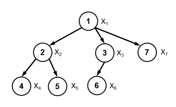
Figure 1: Example of a tree-structured network. Each node has one parent, except for $X_{1}$, the root.

5.1 Tree Structured Network

When the Bayesian network is structured as a tree, each node has exactly one parent, except for the single root. An example of tree-structured network is shown in Figure 1. The following result is a consequence of Theorem 2 specialized to a tree, by noting that each set $\mathsf{par}\left(X_{i}\right)$ is of size $1$, we let $J_{\mathsf{par}\left(i\right)}$ denote $K_{i}$, the cardinality of $\mathsf{par}\left(X_{i}\right)$.

Lemma 10.

Given $0<\epsilon,\delta<1$ and a tree-structured network with $n$ variables, Algorithm NonUniform can continuously maintain an $(\epsilon,\delta)$-approximation to the MLE incurring communication cost $O(\Gamma\cdot\frac{\sqrt{k}}{\epsilon}\cdot\log\frac{1}{\delta}\cdot\log m)$ messages. where $\Gamma=(\sum_{i=1}^{n}(J_{i}J_{\mathsf{par}\left(i\right)})^{2/3})^{3/2}+(\sum_{i=1}^{n}J_{\mathsf{par}\left(i\right)}^{2/3})^{3/2}$. For the case when $J_{i}=J$ for all $i$, this reduces to $\Gamma=O(n^{1.5}J^{2})$.

5.2 Naïve Bayes

The Naïve Bayes model is perhaps the most commonly used graphical model, especially in tasks such as classification, and has a simple structure as shown in Figure 2. The graphical model of Naïve Bayes is a two-layer tree where we assume the root is node $1$.

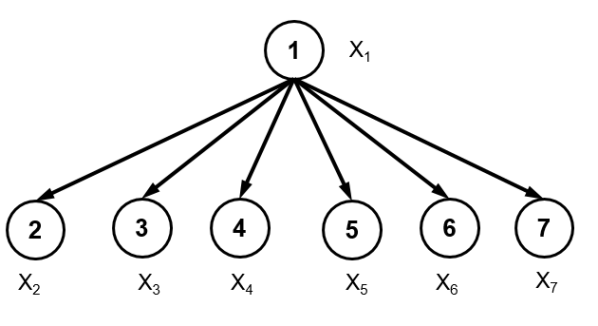
Figure 2: Example of Naïve Bayes over variables $X_{1},X_{2}...,X_{7}$. All the nodes except $X_{1}$ in the graph have the same parent $X_{1}$, which is the root of the tree.

Specializing the NonUniform algorithm for the case of Naïve Bayes, we use results (7) and (8). For each node $X_{i}$ with $i\in[2,n]$, $K_{i}=J_{1}$. Hence, we have the approximation factors ${\tt epsfnA}(i)=\nu_{i}$ and ${\tt epsfnB}(i)=\mu_{i}$ as follows.

$$\nu_{i}={\textstyle{\frac{\epsilon}{16}}}J_{i}^{1/3}\Big{/}\big{(}\sum_{i=2}^{n}J_{i}^{2/3}\big{)}^{1/2},\qquad\mu_{i}=\frac{\epsilon}{16\sqrt{n}}$$ (9)

Note that we maintain the counter $\mathcal{A}_{i}(x_{1})$ for each $x_{1}\in\operatorname{dom}(X_{1})$ and $i\in[2,n]$ independently, as $X_{1}$ is the parent of $X_{2},X_{3},\ldots,X_{n}$. This is wasteful since for $i\in[2,n]$, $\mathcal{A}_{i}(x_{1})$ are all tracking the same event. Utilizing this special structure, we can do better by maintain only one copy of the counter $\mathcal{A}(x_{1})$ for each $x_{1}\in\operatorname{dom}(X_{1})$, but with a more accurate approximation factor $\frac{\epsilon}{3n}$. The resulting algorithm uses Algorithm 4 to perform initialization.

1 foreach $i=2\ldots n$, $x_{i}\in\operatorname{dom}(X_{i})$, and $x_{1}\in\operatorname{dom}(X_{1})$ do

2      $\mathcal{A}_{i}(x_{i},x_{1})\leftarrow$ DistCounter($\nu_{i},\delta$), where $\nu_{i}$ is shown in Equation 9

3foreach $x_{1}\in\operatorname{dom}(X_{1})$ do

4      $\mathcal{A}_{1}(x_{1})\leftarrow$ DistCounter($\frac{\epsilon}{3n},\delta$)

Algorithm 4 Naive-Bayes-Init()

Lemma 11.

Given $0<\epsilon,\delta<1$ and a Naïve Bayes model with $n$ variables, Algorithm 4 combined with Algorithms 2 and 3 continuously maintains an $(\epsilon,\delta)$-approximation to the MLE, incurring communication cost over all the observations $O\left(\frac{\sqrt{k}}{\epsilon}\cdot J_{1}\cdot\left(\sum_{i=2}^{n}J_{i}^{2/3}\right)^{3/2}\cdot\log\frac{1}{\delta}\cdot\log m\right)$ messages over $m$ distributed observations. In the case when all $J_{i}$ are equal to $J$, this expression is $O\left(\frac{n^{3/2}\sqrt{k}}{\epsilon}\cdot J^{2}\cdot\log\frac{1}{\delta}\cdot\log m\right)$.

5.3 Classification

Thus far, our goal has been to estimate probabilities of joint distributions of random variables. We now present an application of these techniques to the task of Bayesian classification. In classification, we are given some evidence $e$, and the objective is to find an assignment to a subset of random variables $Y$, given $e$. The usual way to do this is to find the assignment that maximizes the probability, given $e$. That is, $\text{Class}(\bm{Y}\mid e)=\operatorname*{arg\,max}_{y}{\mathbb{P}}\left[y,e\right]$. We are interested in an approximate version of the above formulation, given by:

Definition 4.

Given a Bayesian Network $\mathcal{G}$, let $Y$ denote the set of variables whose values need to be assigned, and $\epsilon$ denote an error parameter. For any evidence $e$, we say that $\bm{b}$ solves Bayesian classification with $\epsilon$ error if

$$\textstyle\hat{P}\left[Y=\bm{b}\mid e\right]\geq(1-\epsilon)\cdot\max_{y}\hat{P}\left[Y=y\mid e\right].$$

In other words, we want to find the assignment to the set of variables $Y$ with conditional probability close to the maximum, if not equal to the maximum.

Lemma 12.

If for a set of variables $\mathcal{X}=\{X_{1},\ldots,X_{n}\}$, we have $e^{-\epsilon/2}\leq\frac{\tilde{P}\left[\mathcal{X}\right]}{\hat{P}\left[\mathcal{X}\right]}\leq e^{\epsilon/2}$, then for any subset of non-overlapping variables $\bm{X},\bm{Y}\subseteq\mathcal{X}$, $\bm{X}\cap\bm{Y}=\emptyset$, $e^{-\epsilon}\leq\frac{\tilde{P}\left[\bm{Y}\mid\bm{X}\right]}{\hat{P}\left[\bm{Y}\mid\bm{X}\right]}\leq e^{\epsilon}$.

Proof.

For variable set $\bm{X}\subseteq\mathcal{X}$, we have

$$e^{-\epsilon/2}\leq\frac{\tilde{P}\left[\bm{X}\right]}{\hat{P}\left[\bm{X}\right]}\leq e^{\epsilon/2}$$

Similarly, for variable set $\{\bm{X},\bm{Y}\}\subseteq\mathcal{X}$, we have

$$e^{-\epsilon/2}\leq\frac{\tilde{P}\left[\bm{X},\bm{Y}\right]}{\hat{P}\left[\bm{X},\bm{Y}\right]}\leq e^{\epsilon/2}$$

Combining above two inequations,

$$e^{-\epsilon}\leq\frac{\tilde{P}\left[\bm{X},\bm{Y}\right]}{\tilde{P}\left[\bm{X}\right]}\cdot\frac{\hat{P}\left[\bm{X}\right]}{\hat{P}\left[\bm{X},\bm{Y}\right]}\leq e^{\epsilon}$$

Applying Bayes rule, we complete our proof. ∎

Lemma 13.

Given evidence $e$ and set of variables $Y$, if $e^{-\epsilon/4}\leq\frac{\tilde{P}\left[\mathcal{X}\right]}{\hat{P}\left[\mathcal{X}\right]}\leq e^{\epsilon/4}$, then we can find assignment $\bm{b}$ that solves the Bayesian classification problem with $\epsilon$ error.

Proof.

Let $\bm{b}=\operatorname*{arg\,max}_{y}\tilde{P}\left[Y=y\mid e\right]$ and $\bm{b}^{*}=\operatorname*{arg\,max}_{y}\hat{P}\left[Y=y\mid e\right]$. From Lemma 12, we have

$$e^{\epsilon/2}\cdot\hat{P}\left[\bm{Y}=\bm{b}\mid e\right]\geq\tilde{P}\left[\bm{Y}=\bm{b}\mid e\right]$$

As $\bm{b}$ is the most likely assignment for $\tilde{P}\left[Y=y\mid e\right]$,

$$\tilde{P}\left[\bm{Y}=\bm{b}\mid e\right]\geq\tilde{P}\left[\bm{Y}=\bm{b}^{*}\mid e\right]$$

From Lemma 12, for assignment $\bm{b}^{*}$, we have

$$\tilde{P}\left[\bm{Y}=\bm{b}^{*}\mid e\right]\geq e^{-\epsilon/2}\cdot\hat{P}\left[\bm{Y}=\bm{b}^{*}\mid e\right]$$

So we can derive that

$$\hat{P}\left[\bm{Y}=\bm{b}\mid e\right]\geq e^{-\epsilon}\cdot\hat{P}\left[\bm{Y}=\bm{b}^{*}\mid e\right]$$

∎

Theorem 3.

There is an algorithm for Bayesian classification (Definition 4), with communication $O\left(\Gamma\cdot\frac{\sqrt{k}}{\epsilon}\cdot\log\frac{1}{\delta}\cdot\log m\right)$ messages over $m$ distributed observations, where $\Gamma=\left(\sum_{i=1}^{n}(J_{i}K_{i})^{2/3}\right)^{3/2}+\left(\sum_{i=1}^{n}K_{i}^{2/3}\right)^{3/2}$.

Proof.

We use NonUniform to maintain distributed counters with error factor $\frac{\epsilon}{4}$. From Theorem 2, we have $e^{-\epsilon/4}\leq\frac{\tilde{P}\left[\mathcal{X}\right]}{\hat{P}\left[\mathcal{X}\right]}\leq e^{\epsilon/4}$ where $\mathcal{X}$ denote all the variables. Then from Lemma 13, we achieve our goal of Bayesian classification with $\epsilon$ error. ∎

6 Experimental Evaluation

6.1 Setup and Implementation Details

Algorithms were implemented in Java with JDK version 1.8, and evaluated on a 64-bit Ubuntu Linux machine with Intel Core i5-4460 3.2GHz processor and 8GB RAM.

Datasets: We use real-world Bayesian networks from the repository of Bayesian networks at [30]. In our experiments, algorithms assume the network topology, but learn model parameters from training data. Based on the number of nodes in the graph, networks in the dataset are classified into five categories: small networks ($<20$ nodes), medium networks ($20-60$ nodes), large networks ($60-100$ nodes), very large networks ($100-1000$ nodes) and massive networks ($>1000$ nodes). We select one medium network ALARM [31], one large network HEPAR II [32], one very large network LINK [33] and one massive network MUNIN [34]. Table 1 provides an overview of the networks that we use.

Table 1: Bayesian Networks used in the experiments.

Dataset	Number	Number	Number of
	of Nodes	of Edges	Parameters
ALARM [31]	$37$	$46$	$509$
HEPAR II [32]	$70$	$123$	$1453$
LINK [33]	$724$	$1125$	$14211$
MUNIN [34]	$1041$	$1397$	$80592$

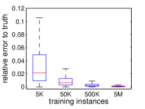
(a) Exact

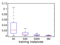
(b) Baseline Approx.

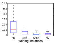
(c) Uniform Approx.

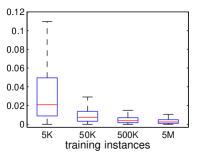
(d) Non-uniform Approx.

Figure 3: Testing error (relative to the ground truth) vs. number of training points. The dataset is HEPAR II.

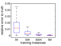
(a) Exact

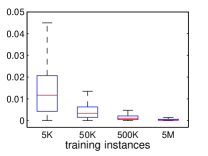
(b) Baseline Approx.

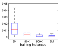
(c) Uniform Approx.

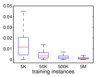
(d) Non-uniform Approx.

Figure 4: Testing error (relative to the ground truth) vs. number of training points. The dataset is LINK.

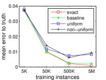
(a) ALARM

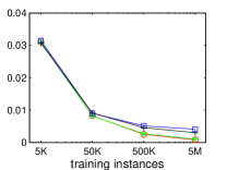
(b) HEPAR II

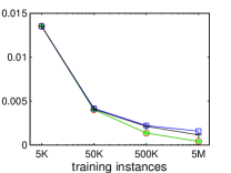
(c) LINK

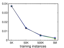
(d) MUNIN

Figure 5: Mean testing error (relative to the ground truth) vs. number of training points.

Training Data: For each network, we generate training data based on the ground truth for the parameters. To do this, we first generate a topological ordering of all vertices in the Bayesian network (which is guaranteed to be acyclic), and then assign values to nodes (random variables) in this order, based on the known conditional probability distributions.

Testing Data: Our testing data consist of a number of queries, each one for the probability of a specific event. We measure the accuracy according to the ability of the network to accurately estimate the probabilities of different events. To do this, we generate $1000$ events on the joint probability space represented by the Bayesian network, and estimate the probability of each event using the parameters that have been learnt by the distributed algorithm. Each event is chosen so that its ground truth probability is at least $0.01$ – this is to rule out events that are highly unlikely, for which not enough data may be available to estimate the probabilities accurately.

Distributed Streams: We built a simulator for distributed stream monitoring, which simulates a system of $k$ sites and a single coordinator. All events (training data) arrive at sites, and queries are posed at the coordinator. Each data point is sent to a site chosen uniformly at random.

Algorithms: We implemented four algorithms: ExactMLE, Baseline, Uniform, and NonUniform. ExactMLE is the strawman algorithm that uses exact counters so that each site informs the coordinator whenever it receives a new observation. This algorithm sends a message for each counter, so that the length of each message exchanged is approximately the same. This makes the measurement of communication cost across different algorithms equivalent to measuring the number of messages. The other three algorithms, Baseline, Uniform, and NonUniform, are as described in Sections 4.3, 4.4, and 4.5 respectively. For each of these algorithms, a message contains an update to the value of a single counter.

Metrics: We compute the probability for each testing event using the approximate model maintained by the distributed algorithm. We compare this with the ground truth probability for the testing event, derived from the ground truth model. For Baseline, Uniform, and NonUniform, we compare their results with those obtained by ExactMLE, and report the median value from five independent runs. Unless otherwise specified, we set $\epsilon=0.1$ and the number of sites to $k=30$.

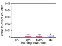
(a) Baseline Approx.

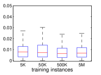
(b) Uniform Approx.

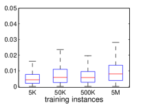
(c) Non-uniform Approx.

Figure 6: Testing error (relative to ExactMLE) vs. number of training points. The dataset is ALARM.

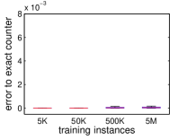
(a) Baseline Approx.

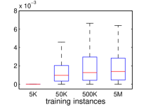
(b) Uniform Approx.

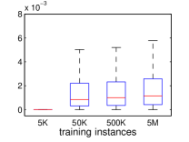
(c) Non-uniform Approx.

Figure 7: Testing error (relative to ExactMLE) vs. number of training points. The dataset is MUNIN.

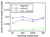
(a) ALARM

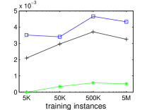
(b) HEPAR II

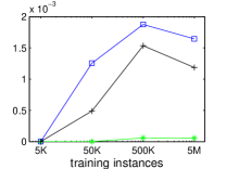
(c) LINK

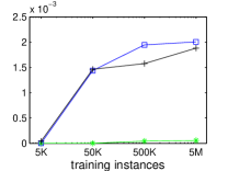
(d) MUNIN

Figure 8: Mean testing error (relative to ExactMLE) vs. number of training points.

6.2 Results and Discussion

The error relative to the ground truth is the average error of the probability estimate returned by the model learnt by the algorithm, relative to the ground truth probability, computed using our knowledge of the underlying model. Figures 3 and 4 respectively show this error as a function of the number of training instances, for the HEPAR II and LINK datasets respectively. As expected, for each algorithm, the median error decreases with an increase in the number of training instances, as can be seen by the middle quantile in the boxplot. The interquartile ranges also shrink with more training instances, showing that the variance of the error is also decreasing.

Figure 5 shows the relative performance of the algorithms. ExactMLE has the best performance of all algorithms, which is to be expected, since it computes the model parameters based on exact counters. Baseline has the next best performance, closely followed by Uniform and NonUniform, which have quite similar performance. Note that the slightly better performance of ExactMLE and Baseline comes at a vastly increased message cost, as we will see next. Finally, all these algorithms achieve good accuracy results. For instance, after $5M$ examples, the error in estimated event probabilities is always less than one percent, for any of these algorithms.

The error relative to the MLE is the average error of the probability estimate returned by the model learnt by the algorithm, relative to the model learnt using exact counters. The distribution of this error is shown for the different algorithms that use approximate counters, in Figures 6 and 7 for the ALARM and MUNIN datasets respectively. The mean error for different algorithms is plotted in Figure 8. We can consider the measured error as having two sources: (1) Statistical error, which is the error in learning that is inherent due to the number of training examples seen so far – this is captured by the error of the model learnt by the exact counter, relative to the ground truth, and (2) Approximation error, which is the difference between the model that we are tracking and the model learnt by using exact counters – this error arises due to our desire for efficiency of communication (i.e., trying to send fewer messages for counter maintenance). Our algorithms aim to control the approximation error, and this error is captured by the error relative to exact counter. We note from the plots that the error relative to exact counter remains approximately the same with increasing number of training points, for all three algorithms, Baseline, Uniform, and NonUniform. This is consistent with theoretical predictions since our algorithms only guarantee that these errors are less than a threshold ($\epsilon$), which does not decrease with increasing number of points. The error of NonUniform is marginally better than that of Uniform. We emphasise that error relative to the ground truth is a more important metric than the error relative to MLE.

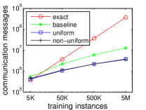
(a) ALARM

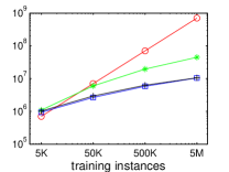
(b) HEPAR II

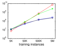
(c) LINK

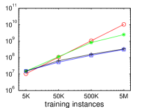
(d) MUNIN

Figure 9: Communication cost vs. number of training points.

Communication cost versus the number of training points for different algorithms is shown in Figure 9. Note that the y-axis is in logarithmic scale. From this graph, we can observe that NonUniform has the smallest communication cost in general, followed by Uniform. These two have a significantly smaller cost than Baseline and ExactMLE. The gap between ExactMLE and NonUniform increases as more training data arrives. For 5M training points, NonUniform sends approximately 100 times fewer messages than ExactMLE, while having almost the same accuracy when compared with the ground truth. This shows the benefit of using approximate counters in maintaining the Bayesian network model. It also shows that there is a concrete and tangible benefit using the improved analysis in Uniform and NonUniform, in reducing the communication cost.

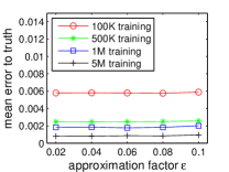
(a) Baseline Approx.

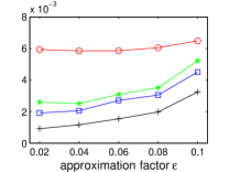
(b) Uniform Approx.

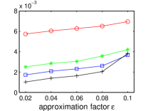
(c) Non-uniform Approx.

Figure 10: Mean testing error (relative to ground truth) vs. approximation factor $\epsilon$. The dataset is HEPAR II.

Figure 10 shows the testing error as a function of the parameter $\epsilon$, and shows that the testing error increases with an increase in $\epsilon$. In some cases, the testing error does not change appreciably as $\epsilon$ increases. This is due to the fact that $\epsilon$ only controls the “approximation error”, and in cases when the statistical error is large (i.e. small numbers of training instances), the approximation error is dwarfed by the statistical error, and the overall error is not sensitive to changes in $\epsilon$.

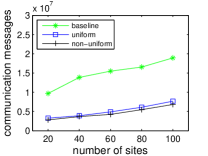
(a) Communication cost for ALARM

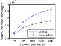
(b) Communication cost for NEW-ALARM

Figure 11: Communication cost experiments.

Last, Figure 11(a) plots communication cost against the number of sites $k$, for the ALARM dataset, and shows that the number of messages increases with $k$.

Communication Cost of Uniform versus NonUniform: The results so far do not show a very large difference in the communication cost of Uniform and NonUniform. The reason is that in the networks that we used, the cardinalities of all random variables were quite similar. In other words, for different $i\in[1,n]$, the $J_{i}$s in Equation 7 and 8 have similar values, and so did the $K_{i}$s. This makes the approximation factors in Uniform and NonUniform to be quite similar. To study the communication efficiency of the non-uniform approximate counter, we generated a semi-synthetic Bayesian network NEW-ALARM based on the ALARM network. We keep the structure of the graph, but randomly choose $6$ variables in the graph and set the size of the universe for these values to $20$ (originally each variable took between $2-4$ distinct values). The format of the synthetic network can be downloaded at [35]. For this network, the communication cost of NonUniform was about 35 percent smaller than that of Uniform, in line with our expectations (Figure 11(b)).

Table 2: Error Rate for Bayesian Classification, $50$K training instances

Dataset	ExactMLE	Baseline	Uniform	NonUniform
ALARM	0.056	0.055	0.053	0.066
HEPAR II	0.191	0.187	0.198	0.212
LINK	0.109	0.110	0.111	0.110
MUNIN	0.091	0.091	0.093	0.091

Table 3: Communication cost to learn a Bayesian classifier

Dataset	ExactMLE	Baseline	Uniform	NonUniform
ALARM	3,700,000	406,721	323,710	322,639
HEPAR II	7,000,000	1,079,385	758,631	754,429
LINK	72,400,000	29,781,937	8223133	8,062,889
MUNIN	104,100,000	34,388,688	11,317,844	11,261,617

Classification: Finally, we show results on learning a Bayesian classifier for our data sets. For each testing instance, we first generate the values for all the variables (using the underlying model), then randomly select one variable to predict, given the values of the remaining variables. We compare the true value and predicted value of the select variable and compute the error rate. $1000$. Prediction error and communication cost for $50$K examples and 1000 tests are shown in Tables 2 and 3 respectively.

Overall, we first note that even the ExactMLE algorithm has some prediction error relative to the ground truth, due to the statistical nature of the model. The error of the other algorithms, such as Uniform and NonUniform is very close to that of ExactMLE, but their communication cost is much smaller. For instance, Uniform and NonUniform send less than $1/9$th as many messages as ExactMLE.

7 Conclusion

We presented new distributed streaming algorithmw to estimate the parameters of a Bayesian Network in the distributed monitoring model. Compared to approaches that maintain the exact MLE, our algorithms significantly reduce communication, while offering provable guarantees on the estimates of joint probability. Our experiments show that these algorithms indeed reduce communication and provide similar prediction errors as the MLE for estimation and classification tasks.

Some directions for future work include: (1) to adapt our analysis when there is a more skewed distribution across different sites, (2) to consider time-decay models which gives higher weight to more recent stream instances, and (3) to learn the underlying graph “live” in an online fashion, as more data arrives.

References

- [1] R. Bekkerman, M. Bilenko, and J. Langford, Scaling Up Machine Learning: Parallel and Distributed Approaches. Cambridge University Press, 2011.
- [2] M. A. et al., “Tensorflow: A system for large-scale machine learning,” in OSDI, 2016, pp. 265–283.
- [3] X. Meng, J. Bradley, B. Yavuz, E. Sparks, and et. al., “MLlib: Machine Learning in Apache Spark,” JMLR, vol. 17, no. 1, pp. 1235–1241, 2016.
- [4] E. P. Xing, Q. Ho, W. Dai, J.-K. Kim, J. Wei, S. Lee, X. Zheng, P. Xie, A. Kumar, and Y. Yu, “Petuum: A new platform for distributed machine learning on big data,” in KDD, 2015, pp. 1335–1344.
- [5] Y. Low, D. Bickson, J. Gonzalez, C. Guestrin, A. Kyrola, and J. M. Hellerstein, “Distributed graphlab: A framework for machine learning and data mining in the cloud,” PVLDB, vol. 5, no. 8, pp. 716–727, Apr. 2012.
- [6] Y. Wang and P. M. Djuric, “Sequential bayesian learning in linear networks with random decision making,” in ICASSP, 2014, pp. 6404–6408.
- [7] J. Aguilar, J. Torres, and K. Aguilar, “Autonomie decision making based on bayesian networks and ontologies,” in IJCNN, 2016, pp. 3825–3832.
- [8] A. T. Misirli and A. B. Bener, “Bayesian networks for evidence-based decision-making in software engineering,” IEEE Trans. Software Eng., vol. 40, no. 6, pp. 533–554, 2014.
- [9] P. Xie, J. H. Li, X. Ou, P. Liu, and R. Levy, “Using bayesian networks for cyber security analysis,” in IEEE/IFIP International Conference on Dependable Systems Networks, 2010, pp. 211–220.
- [10] D. Oyen, B. Anderson, and C. M. Anderson-Cook, “Bayesian networks with prior knowledge for malware phylogenetics,” in Artificial Intelligence for Cyber Security, AAAI Workshop, 2016, pp. 185–192.
- [11] D. Koller and N. Friedman, Probabilistic Graphical Models: Principles and Techniques. MIT Press, 2009.
- [12] G. Cormode, S. Muthukrishnan, and K. Yi, “Algorithms for distributed functional monitoring,” in SODA, 2008, pp. 21:1–21:20.
- [13] M. Balcan, A. Blum, S. Fine, and Y. Mansour, “Distributed learning, communication complexity and privacy,” in PMLR, 2012, pp. 26.1–26.22.
- [14] H. D. III, J. M. Phillips, A. Saha, and S. Venkatasubramanian, “Protocols for learning classifiers on distributed data,” in AISTATS, 2012, pp. 292–290.
- [15] J. Chen, H. Sun, D. P. Woodruff, and Q. Zhang, “Communication-optimal distributed clustering,” in NIPS, 2016, pp. 3720–3728.
- [16] Y. Zhang, J. C. Duchi, M. I. Jordan, and M. J. Wainwright, “Information-theoretic lower bounds for distributed statistical estimation with communication constraints,” in NIPS, 2013, pp. 2328–2336.
- [17] J. M. Phillips, E. Verbin, and Q. Zhang, “Lower bounds for number-in-hand multiparty communication complexity, made easy,” in SODA, 2012, pp. 486–501.
- [18] A. McGregor and H. T. Vu, “Evaluating bayesian networks via data streams,” in COCOON, 2015, pp. 731–743.
- [19] B. Kveton, H. Bui, M. Ghavamzadeh, G. Theocharous, S. Muthukrishnan, and S. Sun, “Graphical model sketch,” in ECML PKDD, 2016, pp. 81–97.
- [20] G. Cormode, “The continuous distributed monitoring model,” SIGMOD Record, vol. 42, no. 1, pp. 5–14, Mar. 2013.
- [21] M. Dilman and D. Raz, “Efficient reactive monitoring,” in INFOCOM, 2001, pp. 1012–1019 vol.2.
- [22] R. Keralapura, G. Cormode, and J. Ramamirtham, “Communication-efficient distributed monitoring of thresholded counts,” in SIGMOD, 2006, pp. 289–300.
- [23] Z. Huang, K. Yi, and Q. Zhang, “Randomized algorithms for tracking distributed count, frequencies, and ranks,” in PODS, 2012, pp. 295–306.
- [24] I. Sharfman, A. Schuster, and D. Keren, “A geometric approach to monitoring threshold functions over distributed data streams,” in SIGMOD, 2006, pp. 301–312.
- [25] ——, “Shape sensitive geometric monitoring,” in PODS, 2008, pp. 301–310.
- [26] G. Cormode, S. Muthukrishnan, and W. Zhuang, “Conquering the divide: Continuous clustering of distributed data streams,” in ICDE, 2007, pp. 1036–1045.
- [27] L. Huang, X. Nguyen, M. Garofalakis, J. Hellerstein, A. D. Joseph, M. Jordan, and N. Taft, “Communication-efficient online detection of network-wide anomalies,” in INFOCOM, 2007, pp. 134–142.
- [28] C. Arackaparambil, J. Brody, and A. Chakrabarti, “Functional monitoring without monotonicity,” in ICALP, 2009, pp. 95–106.
- [29] Y.-Y. Chung, S. Tirthapura, and D. P. Woodruff, “A simple message-optimal algorithm for random sampling from a distributed stream,” IEEE TKDE, vol. 28, no. 6, pp. 1356–1368, Jun. 2016.
- [30] M. Scutari, “Bayesian network repository,” http://www.bnlearn.com/bnrepository/, [Online; accessed May-01-2017].
- [31] I. A. Beinlich, H. J. Suermondt, R. M. Chavez, and G. F. Cooper, “The alarm monitoring system: A case study with two probabilistic inference techniques for belief networks,” in Second European Conference on Artificial Intelligence in Medicine, 1989, pp. 247–256.
- [32] A. Onisko, “Probabilistic causal models in medicine: Application to diagnosis of liver disorders,” Ph.D. dissertation, Polish Academy of Science, Mar. 2003.
- [33] C. S. Jensen and A. Kong, “Blocking gibbs sampling for linkage analysis in large pedigrees with many loops,” The American Journal of Human Genetics, vol. 65, no. 3, pp. 885 – 901, 1999.
- [34] S. Andreassen, F. V. Jensen, S. K. Andersen, B. Falck, U. Kjærulff, M. Woldbye, A. R. Sørensen, A. Rosenfalck, and F. Jensen, “MUNIN — an expert EMG assistant,” in Computer-Aided Electromyography and Expert Systems, 1989.
- [35] “New-alarm bayes network,” https://github.com/yuz1988/new-alarm.