Robustness of clocks to input noise

Abstract

To estimate the time, many organisms, ranging from cyanobacteria to animals, employ a circadian clock which is based on a limit-cycle oscillator that can tick autonomously with a nearly 24h period. Yet, a limit-cycle oscillator is not essential for knowing the time, as exemplified by bacteria that possess an “hourglass”: a system that when forced by an oscillatory light input exhibits robust oscillations from which the organism can infer the time, but that in the absence of driving relaxes to a stable fixed point. Here, using models of the Kai system of cyanobacteria, we compare a limit-cycle oscillator with two hourglass models, one that without driving relaxes exponentially and one that does so in an oscillatory fashion. In the limit of low input noise, all three systems are equally informative on time, yet in the regime of high input-noise the limit-cycle oscillator is far superior. The same behavior is found in the Stuart-Landau model, indicating that our result is universal.

I Introduction

Many organisms, ranging from animals, plants, insects, to even bacteria, possess a circadian clock, which is a biochemical oscillator that can tick autonomously with a nearly 24h period. Competition experiments on cyanobacteria have demonstrated that these clocks can confer a fitness benefit to organisms that live in a rhythmic environment with a 24h period Ouyang:1998wp ; Woelfle:2004cq . Clocks enable organisms to estimate the time of day, allowing them to anticipate, rather than respond to, the daily changes in the environment. While it is clear that circadian clocks which are entrained to their environment make it possible to estimate the time, it is far less obvious that they are the only or best means to do so Roenneberg:2002tt ; Ma:2016ca . The oscillatory environmental input could, for example, also be used to drive a system which in the absence of any driving would relax to a stable fixed point rather than exhibit a limit cycle. The driving would then generate oscillations from which the organism could infer the time. It thus remains an open question what the benefits of circadian clocks are in estimating the time of day.

This question is highlighted by the timekeeping mechanisms of prokaryotes. While circadian clocks are ubiquitous in eukaryotes, the only known prokaryotes to possess circadian clocks are cyanobacteria, which exhibit photosynthesis. The best characterized clock is that of the cyanobacterium Synechococcus elongatus, which consists of three proteins, KaiA, KaiB, and KaiC Ishiura:1998vc . The central clock component is KaiC, which forms a hexamer that is phosphorylated and dephosphorylated in a cyclical fashion under the influence of KaiA and KaiB. This phosphorylation cycle can be reconstitued in the test tube, forming a bonafide circadian clock that ticks autonomously in the absence of any oscillatory driving with a period of nearly 24 hours Nakajima2005 . However, S. elongatus is not the only cyanobacterial species. Prochlorococcus marinus possesses kaiB and kaiC, but lacks (functional) KaiA. Interestingly, this species exhibits daily rhythms in gene expression under light-dark (LD) cycles but not in constant conditions Holtzendorff:2008dj ; Zinser:2009js . Recently, Johnson and coworkers made similar observations for the purple bacterium Rhodopseudomonas palustris, which harbors homologs of KaiB and KaiC. Its growth rate depends on the KaiC homolog in LD but not constant conditions Ma:2016ca , suggesting that the bacterium uses its Kai system to keep time. Moreover, this species too does not exhibit sustained rhythms in constant conditions, but does show daily rhythms in e.g. nitrogen fixation in cyclic conditions. P. marinus and R. palustris thus appear to keep time via an “hourglass” mechanism that relies on oscillatory driving Holtzendorff:2008dj ; Zinser:2009js ; Ma:2016ca . These observations raise the question why some bacterial species like S. elongatus have evolved a bonafide clock that can run freely, while others have evolved an hourglass timekeeping system.

Troein et al. studied the evolution of timekeeping systems in silico Troein:2009bm . They found that only in the presence of seasonal variations and stochastic fluctuations in the input signal did systems evolve that can also oscillate autonomously. However, organisms near the equator have evolved self-sustained oscillations Ma:2016ca , showing that seasonal variations cannot be essential. Pfeuty et al. suggest that limit-cycle oscillators have evolved because they enable timekeepers that ignore the uninformative light-intensity fluctuations during the day (corresponding to a deadzone in the phase-response curve), yet selectively respond to the more informative intensity changes around dawn and dusk Pfeuty:2011em .

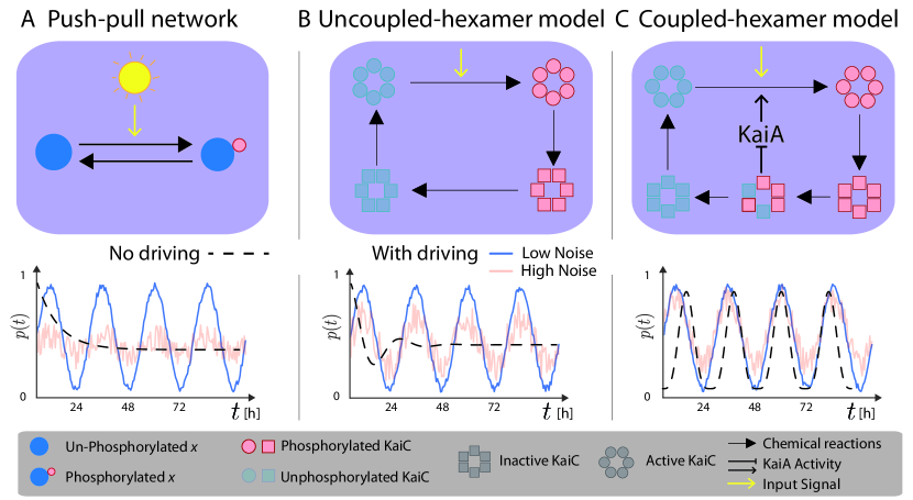
Figure 1: Overview different timekeeping systems. (A) A push-pull network (PPN). Each protein can switch between a phosphorylated and an unphosphorylated state, and the input signal enhances the phosphorylation rate. In the absence of driving, the PPN relaxes exponentially to a steady state (middle panel). Yet, in the presence of an oscillatory input, e.g. sunlight, the system exhibits oscillations from which the time can be inferred (lower panel). (B) The uncoupled-hexamer model (UHM), inspired by the Kai system of P. marinus. It consists of KaiC hexamers which can switch between an active state in which the phosphorylation level tends to rise and an inactive one in which it tends to fall. The phosphorylation rate is, via changes in the ATP/ADP ratio, enhanced by the light input Rust2011 ; Pattanayak:2015jm . The system is akin to a harmonic oscillator, with an intrinsic frequency $\omega_{0}$, resulting from the hexamer phosphorylation cycle. However, the hexamers are not coupled via KaiA as in the CHM shown in panel C, so it cannot sustain autonomous oscillations; in the absence of driving, it relaxes in an oscillatory fashion to a stable fixed point (middle panel). (C) The coupled-hexamer model (CHM), inspired by the Kai system of S. elongatus. Like the UHM, it consists of KaiC hexamers, which tend to be phosphorylated cyclically. However, in contrast to the UHM, the hexamers are synchronized via KaiA, such that the system can exhibit limit-cycle oscillations in the absence of driving (middle panel). In all models, time is estimated from the protein phosphorylation fraction $p(t)$.

Here, we hypothesize that the optimal design of the readout system that maximizes the reliability by which cells can estimate the time depends on the noise in the input signal. To test this idea, we study three different network designs from which the cell can infer time (Fig. 1): 1) a simple push-pull network (PPN), in which a readout protein switches between a phosphorylated and an unphosphorylated state (Fig. 1A). Because the phosphorylation rate increases with the light intensity, the phosphorylation level oscillates in the presence of oscillatory driving, enabling the cell to estimate the time. This network lacks an intrinsic oscillation frequency, and in the absence of driving it relaxes to a stable fixed point in an exponential fashion; 2) an uncoupled hexamer model (UHM), which is inspired by the Kai system of P. marinus (Fig. 1B). This model consists of KaiC hexamers which each have an inherent propensity to proceed through a phosphorylation cycle. However, the phosphorylation cycles of the hexamers are not coupled among each other, and without a common forcing the cycles will therefore desynchronize, leading to the loss of macroscopic oscillations. In contrast to the proteins of the PPN, each hexamer is a tiny oscillator with an intrinsic frequency $\omega_{0}$, which means that an ensemble of hexamers that has been synchronized initially, will, in the absence of driving, relax to its fixed point in an oscillatory manner. 3) a coupled hexamer model (CHM), which is inspired by the Kai system of S. elongatus (Fig. 1C). As in the previous UHM, each KaiC hexamer has an intrinsic capacity to proceed through a phosphorylation cycle, but, in contrast to that system, the cycles of the hexamers are coupled and synchronized via KaiA, as described further below. Consequently, this system exhibits a limit cycle, yielding macroscopic oscillations with intrinsic frequency $\omega_{0}$ even in the absence of any driving.

Here we are interested in the question how the precision of time estimation is limited by the noise in the input signal, and how this limit depends on the architecture of the readout system. We thus focus on the regime in which the input noise dominates over the internal noise Monti:2018hs and model the different systems using mean-field (deterministic) chemical rate equations. In SI , we also consider internal noise, and show that, at least for S. elongatus, the input-noise dominated regime is the relevant limit.

The chemical rate equation of the PPN is: $\dot{x}_{p}=k_{\rm f}s(t)(x_{\rm T}-x_{p}(t))-k_{\rm b}x_{p}(t)$, where $x_{p}(t)$ is the concentration of phosphorylated protein, $x_{\rm T}$ is the total concentration, $k_{\rm f}s(t)$ is the phosphorylation rate $k_{\rm f}$ times the input signal $s(t)$, and $k_{\rm b}$ is the dephosphorylation rate. The uncoupled (UHM) and coupled (CHM) hexamer model are based on the Kai system VanZon2007 ; Rust2007 ; Clodong2007 ; Mori2007a ; Zwicker2010 ; Lin2014 ; Paijmans:2017gx ; Paijmans:2017gp . In both models, KaiC switches between an active conformation in which the phosphorylation level tends to rise and an inactive one in which it tends to fall VanZon2007 ; Lin2014 . Experiments indicate that the main Zeitgeber is the ATP/ADP ratio Rust2011 ; Pattanayak:2015jm , meaning the clock predominantly couples to the input $s(t)$ during the phosphorylation phase of the oscillations Rust2011 ; Paijmans:2017gp . In both the UHM and the CHM, $s(t)$ therefore modulates the phosphorylation rate of active KaiC. The principal difference between the UHM and CHM is KaiA: (functional) KaiA is absent in P. marinus and hence in the UHM Holtzendorff:2008dj ; Zinser:2009js . In contrast, in S. elongatus and hence the CHM, KaiA phosphorylates active KaiC, yet inactive KaiC can bind and sequester KaiA. This gives rise to the synchronisation mechanism of differential affinity VanZon2007 ; Rust2007 ; SI . In all three models, the input is modeled as a sinusoidal signal with mean $\bar{s}$ and driving frequency $\omega=2\pi/T$ plus additive noise $\eta_{s}(t)$: $s(t)=\sin(\omega t)+\bar{s}+\eta_{s}(t)$. The noise is uncorrelated with the mean signal, and has strength $\sigma^{2}_{s}$ and correlation time $\tau_{c}$, $\langle\eta_{s}(t)\eta_{s}(t^{\prime})\rangle=\sigma_{s}^{2}e^{-|t-t^{\prime}|/\tau_{c}}$. A detailed description of the models is given in SI .

As a performance measure for the accuracy of estimating time, we use the mutual information $I(p;t)$ between the time $t$ and the phosphorylation level $p(t)$ Monti:2016bp ; Monti:2018hs :

$$I(p;t)=\int_{0}^{T}dt\int_{0}^{1}dpP(p,t)\log_{2}\frac{P(p,t)}{P(p)P(t)}.$$ (1)

Here $P(p,t)$ is the joint probability distribution while $P(p)$ and $P(t)=1/T$ are the marginal distributions of $p$ and $t$. The quantity $2^{I(p;t)}$ corresponds to the number of time points that can be inferred uniquely from $p(t)$; $I(p;t)=1{\rm bit}$ means that from $p(t)$ the cell can reliably distinguish between day and night Walczak:1324157 . The distributions are obtained from running long simulations of the chemical rate equations of the different models SI .

For each system, to maximize the mutual information we first optimized over all parameters except the coupling strength. For the CHM, the coupling strength $\rho$ was taken to be comparable to that of S. elongatus SI , and for the PPN and the UHM $\rho$ was set to an arbitrary low value, because in the relevant weak-coupling regime the mutual information is independent of $\rho$, as elucidated below and in SI . For the PPN, there exists an optimal response time $\tau_{r}\sim 1/k_{\rm b}$ that maximizes $I(p;t)$, arising from a trade-off between maximizing the amplitude of $p(t)$, which increases with decreasing $\tau_{r}$, and minimizing the noise in $p(t)$, which decreases with increasing $\tau_{r}$ because of time averaging Becker:2015iu ; SI . Similarly, for the UHM, there exists an optimal intrinsic frequency $\omega_{0}$ of the individual hexamers. The UHM is linear and similar to a harmonic oscillator. Analyzing this system shows that while the amplitude $A$ of the output $x(t)$ is maximized at resonance, $\omega_{0}\to\omega$, the standard deviation $\sigma_{x}$ of $x$ is maximized when $\omega_{0}\to 0$, such that the signal-to-noise ratio $A/\sigma_{x}$ peaks for $\omega_{0}>\omega$ SI . Interestingly, also the CHM exhibits a maximum in $A/\sigma_{x}$ for intrinsic frequencies that are slightly off-resonance SI .

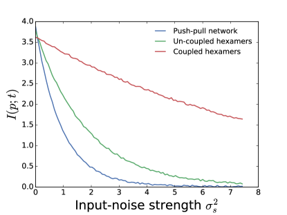
Figure 2: The mutual information $I(p;t)$ as a function of the input-noise strength $\sigma^{2}_{s}$, for the push-pull network (PPN), the uncoupled-hexamer model (UHM) and the coupled-hexamer model (CHM), see Fig. 1. In the limit of low input noise, all systems are equally informative on time, but in the high-noise regime the CHM is most accurate. The parameters have been optimized to maximize $I(p;t)$; since these are (nearly) independent of $\sigma^{2}_{s}$ (Figs.S1-S3), they are fixed (Table S1 SI ).

Fig. 2 shows the mutual information $I(p;t)$ as a function of the input-noise strength $\sigma^{2}_{s}$ for the three systems. In the regime that $\sigma^{2}_{s}$ is small, $I(p;t)$ is essentially the same for all systems. However, the figure also shows that as $\sigma^{2}_{s}$ rises, $I(p;t)$ of the UHM and especially the PPN decrease very rapidly, while that of the CHM falls much more slowly. For $\sigma^{2}_{s}\approx 3$, $I(p;t)$ of the CHM is still above 2 bits, while $I(p;t)$ of the PPN and UHM have already dropped below 1 bit, meaning the cell would no longer be able to distinguish between day and night. Indeed, this figure shows that in the regime of high input noise, a bonafide clock that can tick autonomously is a much better time-keeper than a system which relies on oscillatory driving to show oscillations. This is the principal result of our paper. It is observed for other values of $\tau_{c}$ and other types of input, such as a truncated sinusoid corresponding to no driving at night (Fig. S6 SI ).

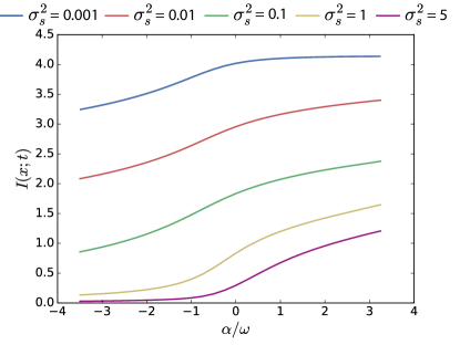
Figure 3: The mutual information $I(p;t)$ as a function of $\alpha$ of the Stuart-Landau model (Eq. 2), for different strengths of the input noise $\sigma^{2}_{s}$. Clearly, $I(p;t)$ rises as the system is changed from a damped oscillator like the UHM ($\alpha<0)$ to a limit-cycle oscillator like the CHM $(\alpha>0)$. Moreover, the increase is most pronounced when $\sigma^{2}_{s}$ is large, as also observed for the UHM and CHM, see Fig. 2. Parameters: $\nu=0$; $\beta=\omega$; $\epsilon=0.5\omega$; $\sigma^{2}_{s}$ in units of $\omega$.

The robustness of our observation that bonafide clocks are more reliable timekeepers, suggests it is a universal phenomenon, independent of the details of the system. We therefore analyzed a generic minimal model, the Stuart-Landau model. It allows us to study how the capacity to infer time changes as a system is altered from a damped (nearly) linear oscillator, which has a characteristic frequency but cannot sustain oscillations in the absence of driving, to a non-linear oscillator that can sustain autonomous oscillations SI . Near a Hopf bifurcation where a limit cycle appears the effect of the non-linearity is weak, so that the solution $x(t)$ is close to that of a harmonic oscillator, $x(t)=1/2(A(t)e^{i\omega t}+c.c.)$, where $A(t)$ is a complex amplitude that can be time-dependent Pikovsky2003 . The dynamics of $A(t)$ is then given by

$$\dot{A} =-i\nu A+\alpha A-\beta|A|^{2}A-\epsilon E,$$ (2)

where $\nu\equiv(\omega^{2}-\omega_{0}^{2})/(2\omega)$ with $\omega_{0}$ the intrinsic frequency, $\alpha$ and $\beta$ govern the linear and non-linear growth and decay of oscillations, $E$ is the first harmonic of $s(t)$ and $\epsilon\equiv\rho/(2\omega)$ is the coupling strength. Eq. 2 gives a universal description of a driven weakly non-linear oscillator near a supercritical Hopf bifurcation Pikovsky2003 .

The non-driven system exhibits a Hopf bifurcation at $\alpha=0$. By varying $\alpha$ we can thus change the system from a damped oscillator ($\alpha<0)$ which in the absence of driving exhibits oscillations that decay, to a limit-cycle oscillator ($\alpha>0$) that shows free-running oscillations. The driven damped oscillator ($\alpha<0$) always has one stable fixed point with $|A|>0$ corresponding to sinusoidal oscillations that are synchronized with the driving. The driven limit-cycle oscillator ($\alpha>0$), however, can exhibit several distinct dynamical regimes Pikovsky2003 . Here, we limit ourselves to the case of perfect synchronization, where $x(t)$ has a constant amplitude $A$ and phase shift with respect to $s(t)$.

To compute $I(x,t)$, we use an approach inspired by the linear-noise approximation Monti:2018hs . It assumes $P(x|t)$ is a Gaussian distribution with variance $\sigma^{2}_{x}(t)$ centered at the deterministic solution $x(t)=1/2(Ae^{i\omega t}+c.c.)$, where $A$ is obtained by solving Eq. 2 in steady state. To find $\sigma^{2}_{x}$, we first compute $\sigma^{2}_{A}$ from Eq. 2 by adding Gaussian white-noise of strength $\sigma^{2}_{s}$ to $E$ and expanding $A$ to linear order around its fixed point; $\sigma^{2}_{x}(t)$ is then obtained from $\sigma^{2}_{A}$ via a coordinate transformation SI .

Fig. 3 shows the mutual information $I(x;t)$ as a function $\alpha$, for different values of $\sigma^{2}_{s}$. The figure shows that $I(x;t)$ rises as the system is changed from a damped oscillator ($\alpha<0$) to a self-sustained oscillator ($\alpha>0$). Moreover, the increase is most pronounced when the input noise $\sigma^{2}_{s}$ is large. The Stuart-Landau model can thus reproduce the qualitative behavior of our computational models, indicating that our principal result is generic. Interestingly, the CHM is even more robust to input noise than the Stuart-Landau model, likely because the latter is only weakly non-linear.

To understand why limit-cycle oscillators are more robust to input noise, we study in section SIIE SI analytical models valid in the limit of weak coupling. For a damped oscillator with a fixed-point attractor (PPN and UHM), we find that the amplitude $A$ of the harmonic oscillations (the signal) increases with the coupling strength $\rho$, $A\sim\rho$. The noise in the output signal $\sigma_{x}$ scales with $\rho$, $\sigma_{x}\sim\rho$, because the coupling amplifies not only the input signal, but also the input noise. Hence, the signal-to-noise ratio $A/\sigma_{x}$ is independent of $\rho$: an oscillator based on a fixed-point attractor faces a fundamental trade-off between gain and input noise (section SIIE SI ). A limit-cycle oscillator (CHM) can lift this trade-off: The amplitude is a robust, intrinsic property of the system, and essentially independent of $\rho$. The output noise $\sigma_{x}\sim\sqrt{\rho}$, because the coupling not only amplifies the input noise proportional to $\rho$, but also generates a restoring force that constrains fluctuations, scaling as $\sim\sqrt{\rho}$ (SIIE SI ). Hence, $A/\sigma_{x}\sim 1/\sqrt{\rho}$. These scaling arguments show that: 1) concerning robustness to input noise, the optimal regime is the weak-coupling regime; 2) in this regime, a limit-cycle oscillator is generically more robust to input noise than a damped oscillator.

Yet, the coupling cannot be reduced to zero for limit-cycle oscillators. When the intrinsic clock period deviates from 24h, as it typically will, coupling is essential to phase-lock the clock to the driving signal Monti:2018hs . Moreover, biochemical networks inevitably have some level of internal noise (section SIIF SI ). For the damped oscillator, the output noise $\sigma_{x}$ resulting from internal noise is independent of $\rho$, but since $A$ increases with $\rho$, $A/\sigma_{x}\sim\rho$ in the presence of internal noise only: coupling helps to lift the signal above the internal noise. For the limit-cycle oscillator, the restoring force $\sim\sqrt{\rho}$ tames phase diffusion, such that in the presence of only internal noise, the output noise $\sigma_{x}\sim 1/\sqrt{\rho}$ and $A/\sigma_{x}\sim\sqrt{\rho}$. Hence, also with regards to internal noise, a limit-cycle oscillator is superior to a damped oscillator in the weak-coupling regime. This analysis also shows, however, that this regime is not necessarily optimal, since with only internal noise present $A/\sigma_{x}$ increases with $\rho$. In fact, it predicts that in the strong-coupling regime the damped oscillator outperforms the limit-cycle oscillator. We emphasize, however, that in this regime our weak-coupling analysis breaks down and other effects come into play; for example, non-linearities arising from the bounded character of $p(t)$ distort the signal, reducing information transmission.

In the presence of both noise sources, we expect an optimal coupling that maximizes information transmission (SIIF SI ). For the limit-cycle oscillator the optimum arises from the trade-off between minimizing input-noise propagation and maximizing internal-noise suppression. For the damped oscillator, $A/\sigma_{x}$ first rises with $\rho$ because coupling helps to lift the signal above the internal noise, but then plateaus when the input noise (which increases with $\rho$) dominates over the internal noise; for even higher $\rho$, it decreases again because of signal distortion. In section SIE SI we verify these predictions for our computational models using stochastic simulations.

Experiments have shown that the clock of S. elongatus has a strong temporal stability with a correlation time of several months Mihalcescu:2004ch , suggesting that the internal noise is small. Indeed, typical input-noise strengths based on weather data Gu:2001vh and internal-noise strengths based on protein copy numbers in S. elongatus Kitayama:2003un indicate that in the biologically relevant regime, at least for cyanobacteria, input noise dominates over internal noise (Fig. S5 SI ). In this regime, the focus of our paper, the optimal coupling is weak and limit-cycle oscillators are generically more robust to input noise than damped oscillators.

This work is part of the research programme of the Netherlands Organisation for Scientific Research (NWO) and was performed at AMOLF. DKL acknowledges NSF grant DMR 1056456 and grant PHY 1607611 to the Aspen Center for Physics, where part of this work was completed. We thank Jeroen van Zon and Nils Becker for a critical reading of the manuscript.

Supplemental Material:
Robustness of circadian clocks to input noise

This supporting information provides background information on the computational models and analytical models that we have studied. The computational models are described in the next section, while the analytical models are discussed in section SII.

SI Computational Models

In this section, we describe the three computational models that we have considered in this study: the push-pull network; the uncoupled-hexamer model; and the coupled-hexamer model. We also describe how we have modeled the input signal and how the systems are coupled to the input. As described in the main text, we are interested in the question how the robustness to input noise depends on the architecture of the readout system; we therefore model these systems with deterministic mean-field chemical rate equations. However, here in the Supporting Information we also test how robust our findings are, not only to the shape of the input signal, but also to the presence of internal noise.

In the next section, we first describe how we have modeled the input signal. In the subsequent sections, we then describe the deterministic computational models, how they are coupled to the input, and how we have set their parameters. Table S1 lists the values of all the parameters of all the models. In section SI.5 we show that the principal findings of Fig.2 are robust to the presence of internal noise and in section SI.6 we show that they are robust to the type of input signal and the noise correlation time.

SI.1 Input signal

The input signal is modeled as a sinusoidal oscillation with additive noise:

$$s(t)=\sin(\omega t)+\bar{s}+\eta_{s}(t),$$ (S1)

where $\bar{s}$ is the mean input signal and $\eta_{s}(t)$ describes the input noise. The noise in the input is assumed to be uncorrelated with the mean input signal $s(t)$. Moreover, we assume that the input noise has strength $\sigma^{2}_{s}$ and is colored, relaxing exponentially with correlation time $\tau_{c}$: $\langle\eta_{s}(t)\eta_{s}(t^{\prime})\rangle=\sigma^{2}_{s}e^{-|t-t^{\prime}|/\tau_{c}}$.

The input signal $s(t)$ is coupled to the system by modulating the phosphorylation rate $k_{\alpha}$ of the core clock protein, as we describe in detail for the respective computational models in the next sections. Here, $k_{\alpha}=k_{\rm f},k_{\rm ps},k_{i}$, depending on the computational model. As we will see, the net phosphorylation rate is given by

$$k_{\alpha}s(t) =k_{\alpha}s(t)$$ (S2)

$$=k_{\alpha}\bar{s}+k_{\alpha}\left(\sin(\omega t)+\eta_{s}\right).$$ (S3)

This expression shows that in the presence of oscillatory driving, the mean phosphorylation rate averaged over a period is set by $k_{\alpha}\bar{s}$, while the amplitude of the oscillation in the phosphorylation rate, which sets the strength of the forcing, is given by $k_{\alpha}$. We also note that $k_{\alpha}$ amplifies not only the “true” signal $\sin(\omega t)$, but also the noise $\eta_{s}$, the consequences of which will be discussed below. Lastly, the absence of any oscillatory driving is modeled by taking $s(t)=\bar{s}$, such that the net phosphorylation rate is then $k_{\alpha}\bar{s}$. The phosphorylation rate in the presence of stochastic driving is thus characterized by the following parameters: the mean phosphorylation rate $k_{\alpha}\bar{s}$, the amplitude of the phosphorylation-rate oscillations $k_{\alpha}$, and the noise $\eta_{s}(t)$, characterized by the noise strength $\sigma^{2}_{s}$ and correlation time $\tau_{c}$. We will vary $\sigma^{2}_{s}$ and $\tau_{c}$ systematically, while $\bar{s}$ and $k_{\alpha}$, together with the other system parameters, will be optimized to maximize the mutual information, as described below.

While we will vary $\sigma^{2}_{s}$, weather data gives us ball-park estimates for the typical input-noise strengths. The weather data of Gu:2001vh indicates that the average relative noise intensity at noon is around $\langle\delta I^{2}\rangle/\langle I\rangle^{2}\approx 0.2-0.3$, which corresponds to $\sigma^{2}_{s}/\bar{s}^{2}$ in our model, yielding $\sigma^{2}_{s}\approx 1-2$ for the baseline parameter value of the mean signal $\bar{s}=2$ (see Table S1). Because there will be variations in the fluctuations in the light intensity from day-to-day, we will also study higher values of the input noise.

In the simulations, realisations of $\eta_{s}(t)$ are generated via the Ornstein-Uhlenbeck process

$$\dot{\eta}_{s} =-\eta_{s}/\tau_{c}+\xi(t),$$ (S4)

where $\xi(t)$ is Gaussian white noise $\langle\xi(t)\xi(t^{\prime})\rangle=\langle\xi^{2}\rangle\delta(t-t^{\prime})$. This generates colored noise of $\eta_{s}(t)$, $\langle\eta_{s}(t)\eta_{s}(t^{\prime})\rangle=\sigma^{2}_{s}e^{-|t-t^{\prime}|/\tau_{c}}$, where $\sigma^{2}_{s}=\langle\xi^{2}\rangle\tau_{c}/2$.

The results of Fig. 2 of the main text correspond to $\tau_{c}=0.5/{\rm h}$, consistent with the weather data of Gu:2001vh . However, we have tested the robustness of the results by varying the noise correlation time $\tau_{c}$. In addition, to test the robustness of our observations to changes in the shape of the input signal, we have also varied that. These tests are described in section SI.6 and the results are shown in Fig. S6. Clearly, the principal result of Fig. 2 of the main text is robust to changes in both the noise correlation time $\tau_{c}$ and the shape of the mean-input signal.

Parameter	Description	Value
Push-pull network, Eq. S5
$k_{\rm f}$	Phosphorylation rate	$0.01/{\rm h}$
$k_{\rm b}$	Dephosphorylation rate (Eq. S45)	$0.3/{\rm h}$
Uncoupled-hexamer model, Eqs. S6-S11
$k_{\rm f}$	Phosphorylation rate	$0.26/{\rm h}$
$k_{\rm b}$	Dephosphorylation rate	$0.52/{\rm h}$
$k_{\rm s}$	Conformational switching rate	$100/{\rm h}$
Coupled-hexamer model, Eqs. S14-S20
$k_{\rm ps}$	Autophosphorylation rate	$0.0125/{\rm h}$
$k_{\rm b}$	Dephosphorylation rate	$0.1875/{\rm h}$
$k_{\rm s}$	Conformational switching rate	$100/{\rm h}$
$K_{0}$	KaiA dissociation constant ${\rm C}_{0}$	$0.0001$
$K_{1}$	KaiA dissociation constant ${\rm C}_{1}$	$0.0003$
$K_{2}$	KaiA dissociation constant ${\rm C}_{2}$	$0.001$
$K_{3}$	KaiA aissociation constant ${\rm C}_{3}$	$0.003$
$K_{4}$	KaiA dissociation constant ${\rm C}_{4}$	$0.01$
$K_{5}$	KaiA dissociation constant ${\rm C}_{5}$	$0.03$
$k_{0}$	KaiA-stimulated phosphorylation rate ${\rm C}_{0}$	$0.5/{\rm h}$
$k_{1}$	KaiA-stimulated phosphorylation rate ${\rm C}_{1}$	$0.5/{\rm h}$
$k_{2}$	KaiA-stimulated phosphorylation rate ${\rm C}_{2}$	$0.5/{\rm h}$
$k_{3}$	KaiA-stimulated phosphorylation rate ${\rm C}_{3}$	$0.5/{\rm h}$
$k_{4}$	KaiA-stimulated phosphorylation rate ${\rm C}_{4}$	$0.5/{\rm h}$
$k_{5}$	KaiA-stimulated phosphorylation rate ${\rm C}_{5}$	$0.5/{\rm h}$
$\tilde{b}_{2-4}$	Number KaiA dimers sequestered by $\tilde{\rm C}_{1-4}$	$2$
$\tilde{b}_{0,5,6}$	Number KaiA dimers sequestered by $\tilde{\rm C}_{0,5,6}$	0
$\tilde{K}_{1-4}$	KaiA dissociation constant $\tilde{\rm C}_{1-4}$	0.000001
$\tilde{K}_{0,5,6}$	KaiA dissociation constant $\tilde{\rm C}_{0,5,6}$	$\infty$
$c_{\rm T}$	Total concentration of KaiC	$1$
$A_{\rm T}$	Total concentration of KaiA	$1$

Table S1: Parameter values of all the three computational models studied in the main text. The parameter values listed are those that maximize the mutual information $I(p;t)$ between the phosphorylation level $p$ and time $t$; these values are nearly independent of the input-noise strength $\sigma^{2}_{s}$, and thus kept constant as $\sigma^{2}_{s}$ is varied in the simulations corresponding to Fig. 2 of the main text. For these optimal parameters values, the intrinsic period of the uncoupled-hexamer model is $T_{0}^{\rm opt}\approx 23.1{\rm h}$ while that of the coupled-hexamer model is $T_{0}^{\rm opt}\approx 25.1{\rm h}$. All three models are coupled to the input by multiplying the phosphorylation rates with $s(t)=\sin(\omega)+\bar{s}+\eta_{s}(t)$, where $\bar{s}=2$ and $\eta_{s}(t)$ describes colored noise with strength $\sigma^{2}_{s}$ and correlation time $\tau_{c}$, $\langle\eta_{s}(t)\eta_{s}(t^{\prime})\rangle=\sigma^{2}_{s}e^{-|t-t^{\prime}|/\tau_{c}}$. For Fig. 2 of the main text, $\tau_{c}=0.5{\rm h}$. Dissociation constants and protein concentrations are in units of the total KaiC concentration. Note that in the absence of oscillatory driving $s(t)=\bar{s}=2$, meaning that in simulations of the non-driven systems the phosphorylation rates $k_{\rm f}$, $k_{i}$, $k_{\rm ps}$, still have to be multiplied by $\bar{s}=2$.

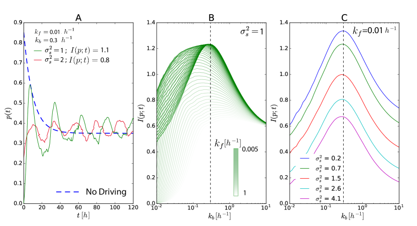
Figure S1: The deterministic push-pull network. (A) Time traces of $p(t)$ in the absence of driving (dashed line) and in the presence of driving (solid lines), for two different values of the input-noise strength $\sigma^{2}_{s}$; the corresponding values of the mutual information $I(p;t)$ are also shown. Note that in the absence of driving, the system relaxes in an exponential fashion to a stable fixed point. (B) The mutual information $I(p;t)$ as a function of $k_{\rm b}$ for different values of $k_{\rm f}$ (see Eq. S5), for $\sigma^{2}_{s}=1$. It is seen that for each phosphorylation rate $k_{\rm f}$ there is an optimal dephosphorylation rate $k_{\rm b}$ that maximizes the mutual information $I(p;t)$. Moreover, $I(p;t)$ increases as $k_{\rm f}$ decreases, but then saturates and hence becomes independent of $k_{\rm f}$ as the system enters the regime in which it responds linearly to the input $s$. The dashed line shows the optimal value of $k_{\rm b}^{\rm opt}\approx 0.3/{\rm h}$, as predicted by Eq. S45. (C) The mutual information $I(p;t)$ as a function of the dephosphorylation rate $k_{\rm b}$, for different values of the input-noise strength $\sigma^{2}_{s}$, keeping the phosphorylation rate fixed at $k_{\rm f}=0.01/{\rm h}$. The optimal dephosphorylation rate $k_{\rm b}^{\rm opt}\approx 0.3/{\rm h}$ (dashed line) is independent of $\sigma^{2}_{s}$, as predicted by Eq. S45. The input-noise correlation time $\tau_{c}=0.5{\rm h}$.

SI.2 Push-pull network

The deterministic push-pull network is described by the following reaction

$$\dot{x}_{p}=k_{\rm f}s(t)(x_{\rm T}-x_{p}(t))-k_{\rm b}x_{p}(t),$$ (S5)

where $x_{\rm T}=x+x_{p}$ is the total protein concentration, $x_{p}$ is the concentration of phosphorylated protein, $k_{\rm f}s(t)$ is the phosphorylation rate $k_{\rm f}$ times the input signal $s(t)$ (see Eq. S1) and $k_{\rm b}$ is the dephosphorylation rate. Fig. S1A shows a time trace of both a driven and a non-driven push-pull network.

Setting the parameters
The steady-state mean phosphorylation level is set by $\bar{p}=\bar{x}_{p}/x_{T}=k_{\rm f}\bar{s}/(k_{\rm f}\bar{s}+k_{\rm b})$. We anticipated, based on the analytical calculations described in section SII.1, that a key timescale is $k_{\rm b}$ and that the system should operate in the regime in which it responds linearly to changes in the mean input $\bar{s}$. This means that for a given $k_{\rm b}$, $k_{\rm f}$ and $\bar{s}$ cannot be too large. We have chosen $\bar{s}=2$, and then varied $k_{\rm f}$ and $k_{\rm b}$ to optimize the mutual information. We then verified a posteriori that the value of $\bar{s}=2$ indeed puts the system in the optimal linear regime.

Optimal dephosphorylation rate Specifically, the parameters $k_{\rm f}$ and $k_{\rm b}$ are set as follows: for a given input noise strength $\sigma^{2}_{s}=1.0$, we first fix the phosphorylation rate $k_{\rm f}$ and compute the mutual information $I(p;t)$ between the phosphorylated fraction $p(t)=x_{p}(t)/x_{T}$ and time $t$ as a function of the dephosphorylation rate $k_{b}$; we then repeat this procedure by varying $k_{\rm f}$. The result is shown in Fig. S1B. Clearly, there exists an optimal value of $k_{\rm b}$ that maximizes $I(p;t)$. Moreover, the optimal value $k_{\rm b}^{\rm opt}$ becomes indepdendent of $k_{\rm f}$ when $k_{\rm f}$ becomes so small that the system enters the regime in which it responds linearly to changes in the mean input $\bar{s}$. We then fixed the phosphorylation rate to $k_{\rm f}=0.01/{\rm h}$, and compute $I(p;t)$ as a function of $k_{\rm b}$ for different levels of the input-noise strength, see Fig. S1C. It is seen that the optimal dephosphorylation rate $k_{\rm b}^{\rm opt}$ is essentially independent of the input noise strength $\sigma^{2}_{s}$. In the simulations corresponding to Fig. 2 of the main text, we therefore kept $k_{\rm b}$ constant at $k_{\rm b}^{\rm opt}=0.3/{\rm h}$ and $k_{\rm f}$ constant at $k_{\rm f}=0.01/{\rm h}$ when we varied $\sigma^{2}_{s}$.

The observation that $k_{\rm b}^{\rm opt}$ is independent of $k_{\rm f}$ and $\sigma^{2}_{s}$ can be understood by noting that to maximize information transmission, the system should operate in the linear-response regime in which the mean output $\bar{x}$ responds linearly to changes in the mean input $\bar{s}$. This regime tends to enhance information because it ensures that in the presence of a sinusoidal input, the output $x_{p}(t)$ will not be distorted and be sinusoidal too. In this linear-response regime, the system can be analyzed analytically, see Eq. S45 in section SII.1 below. This equation, which accurately predicts the optimum seen in Fig. S1B and Fig. S1C, reveals that the optimal dephosphorylation rate depends on the frequency of the driving signal, $\omega$, and the correlation time of the noise, $\tau_{c}$, but not on the noise strength $\sigma^{2}_{s}$ and the coupling $\rho$ to the input signal, given by $\rho=k_{\rm f}x_{T}$. Increasing the gain $\rho$ amplifies not only the true signal, but also the noise in that signal (see also Eq. S3), such that the signal-to-noise ratio is unaltered. Indeed, increasing the gain only helps in the presence of internal noise, which here and the main text, however, is zero.

In sections SI.5 and SII.6 we discuss the role of internal noise. As Fig. S4 shows, in the presence of not only input noise but also internal noise, there exists an optimal, non-zero, coupling strength, which arises as a trade-off between lifting the amplitude of the output above the internal noise (which necessitates a sufficiently large coupling strength, see Eq. S124) and minimizing the distortions of the shape of the output signal. However, for biologically relevant copy numbers the internal noise is small, while signal distortions only kick in at large coupling strengths. Consequently, the optimum is broad (Fig. S4). The chosen coupling strength here is in the plateau regime in which the mutual information is maximized in the presence of both internal and input noise.

SI.3 Uncoupled-hexamer model: Kai system of Prochlorococcus

Background The uncoupled-hexamer model (UHM) presented in the main text is a minimal model of the Kai system of the cyanobacterium Proclorococcus and, possibly, the purple bacterium Rhodopseudomonas palustris. The well characterized clock of the cyanobacterium S. elongatus consists of three proteins, KaiA, KaiB and KaiC, which are all essential for sustaining free-running oscillations Ishiura:1998vc . And, indeed, many cyanobacteria possess at least one copy of each kai gene. One exception is Proclororoccus, which contains kaiB and kaiC, but misses a (functional) kaiA gene. Interestingly, in daily (12h:12h) light-dark (LD) cycles, the expression of many genes, including kaiB and kaiC, is rhythmic, but in constant conditions these rhythms damp very rapidly Holtzendorff:2008dj ; Zinser:2009js . Similar behavior is observed for the purple bacterium R. palustris, which possesses homologs of the kaiB and kaiC genes Ma:2016ca : under LD conditions, the KaiC homolog appears to be phosphorylated in a circadian fashion, but under constant conditions, the oscillations decay very rapidly; physiological activities, such as the nitrogen fixation rates, follow a similar pattern Ma:2016ca . Of particular interest is the observation that under LD conditions but not under LL conditions, the growth rate is significantly reduced in the strain in which the kaiC homolog was knocked out Ma:2016ca . This strongly suggests that the (homologous) Kai system plays a role as a timekeeping mechanism, which relies, however, on oscillatory driving.

Model Our model is inspired by the models that in recent years have been developed for S. elongatus VanZon2007 ; Rust2007 ; Zwicker2010 ; Lin2014 ; Paijmans:2017gx . These models share a number of characteristics that are essential for generating oscillations and entrainment (see also next section). The central clock component is KaiC, a hexamer, that can switch between an active state in which the phosphorylation level tends to rise and an inactive one in which it tends to fall. The model lacks KaiA because Proclororoccus and R. palustris miss a functional kaiA gene Holtzendorff:2008dj ; Zinser:2009js ; Ma:2016ca . In S. elongatus, KaiB does not directly affect the rates of phosphorylation and dephosphorylation, but mainly serves to stabilize the inactive state and mediate KaiA binding by inactive KaiC Lin2014 ; Paijmans:2017gx . KaiB is therefore not modelled explicitly Lin2014 ; Paijmans:2017gx . The main entrainment signal for S. elongatus is the ratio of ATP to ADP levels, which depends on the light intensity, and predominantly couples to KaiC in its active conformation Rust2011 ; Pattanayak:2015jm ; Paijmans:2017gx ; Paijmans:2017gp . These observations give rise to the following chemical rate equations of our deterministic model:

$$\dot{c}_{0} =k_{\rm s}\tilde{c}_{0}-k_{\rm f}s(t)c_{0}$$ (S6)

$$\dot{c}_{i} =k_{\rm f}s(t)(c_{i-1}-c_{i}) i\in(1,\dots,5)$$ (S7)

$$\dot{c}_{6} =k_{\rm f}s(t)c_{5}-k_{\rm s}c_{6}$$ (S8)

$$\dot{\tilde{c}}_{6} =k_{\rm s}c_{6}-k_{\rm f}\tilde{c}_{6}$$ (S9)

$$\dot{\tilde{c}}_{i} =k_{\rm b}(\tilde{c}_{i+1}-\tilde{c}_{i}) i\in(1,\dots,5)$$ (S10)

$$\dot{\tilde{c}}_{0} =k_{\rm b}\tilde{c}_{1}-k_{\rm s}\tilde{c}_{0}$$ (S11)

Here, $c_{i}$, with $i=0,\dots,6$, is the concentration of active $i$-fold phosphorylated KaiC in its active conformation, while $\tilde{c}_{i}$ is the concentration of inactive $i$-fold phosphorylated KaiC. The quantity $k_{\rm s}$ is the conformational switching rate, $k_{\rm b}$ is the dephosphorylation rate of inactive KaiC, and $k_{\rm f}s(t)$ is the phosphorylation rate of active KaiC, $k_{\rm f}$, times the input signal $s(t)$.

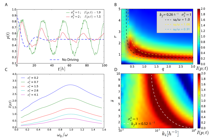
Figure S2: The deterministic uncoupled-hexamer model. (A) Time traces of $p(t)$ in the absence of driving (dashed line) and in the presence of driving (solid lines), for two different values of the input-noise strength $\sigma^{2}_{s}$; the corresponding values of the mutual information $I(p;t)$ are also shown. Note that in the absence of driving, the system relaxes in an oscillatory fashion to a stable fixed point. (B) Heatmap of the mutual information $I(p;t)$ as a function of the scaling factor ${q}$ that scales both the dephosphorylation rate $k_{\rm b}$ and the the mean phosphorylation rate $k_{\rm f}\bar{s}$ (see Eq. S3) and the ratio ${r}=k_{\rm b}/(k_{\rm f}\bar{s})$ of these quantities. The mean phosphorylation rate $k_{\rm f}\bar{s}$ is changed by varying $k_{\rm f}$ while keeping $\bar{s}=2$ constant. Superimposed are contour lines of constant $\omega_{0}=\omega_{0}(q,r)$ (see Eq. S13). It is seen that in the regime where $I(p;t)$ is high, $I(p,t)$ is almost constant along these contour lines, showing that $I(p;t)$ predominantly depends on $k_{\rm f}$ and $k_{\rm b}$ via $\omega_{0}$. (C) The mutual information $I(p;t)$ as a function of $\omega_{0}$, which was varied by scaling $k_{\rm f}$ and $k_{\rm b}$ keeping $r=k_{\rm b}/(k_{\rm f}\bar{s})=1$ and $\bar{s}=2$, for different values of the input-noise strength $\sigma^{2}_{s}$. It is seen that there exists an optimal intrinsic frequency $\omega_{0}^{\rm opt}$ that maximizes $I(p;t)$. Moreover, $\omega_{0}^{\rm opt}$ is nearly independent of $\sigma^{2}_{s}$, corresponding to an intrinsic period $T_{0}=2\pi/\omega_{0}^{\rm opt}\approx 23.1{\rm h}$. (D) The mutual information $I(p;t)$ as a function of $k_{\rm f}$ and $\bar{s}$, keeping $k_{\rm b}=0.52/{\rm h}$ constant. Superimposed is the line along which $k_{\rm f}\bar{s}=k_{\rm b}=0.52/{\rm h}$ is constant and hence the intrinsic period $T_{0}$ is constant (see Eq. S13) and equal to $T_{0}=23.1{\rm h}$. Along this line also $I(p;t)$ is essentially constant, meaning that the strength of the forcing, set by $k_{\rm f}$, is not very critical. This mirrors the behavior seen for the push-pull network (see Fig. S1). It is due to the fact that increasing the forcing raises not only the amplitude but also the noise, keeping the signal-to-noise ratio and hence the mutual information essentially unchanged. The noise correlation time $\tau_{c}=0.5{\rm h}$.

The output is the phosphorylation fraction of KaiC proteins (monomers), given by VanZon2007 ; Zwicker2010 ; Paijmans:2017gx

$$p(t)=\frac{1}{6}\frac{\sum_{i=0}^{6}i(c_{i}+\tilde{c}_{i})}{\sum_{i=0}^{6}(c_{i}+\tilde{c}_{i})}.$$ (S12)

Fig. S2A shows a time trace of the phosphorylation level $p(t)$ of both a driven and a non-driven uncoupled-hexamer model.

Intrinsic frequency Because the cycles of the different hexamers are not coupled via KaiA as in the coupled-hexamer model and in S. elnogatus, the system cannot sustain free-running oscillations. In this respect, the system is similar to the push-pull network in the sense that a perturbation of the non-driven system will relax to a stable fixed point. However, this model differs from the push-pull network in that it has a characteristic frequency $\omega_{0}=2\pi/T_{0}$ with intrinsic period $T_{0}$, arising from the phosphorylation cycle of the KaiC hexamers. Consequently, while a perturbed (non-driven) push-pull network will relax exponentially to its stable fixed point, the uncoupled-hexamer model will, when not driven, relax in an oscillatory fashion to its stable fixed point with an intrinsic frequency $\omega_{0}$ (see Fig. S2A). To predict the latter, we note that the dynamics of Eqs. S6-S11 can be written in the form $\dot{\bf x}={\bf A}{\bf x}$, and when all rate constants are equal, $k_{\rm f}\bar{s}=k_{\rm b}=k_{\rm s}$, the eigenvalues and eigenvectors of ${\bf A}$ can be computed analytically. The eigenvectors are complex exponentials. For a cycle with $N$ sites with hopping rate $k$, the frequency associated with the lowest-lying eigenvalue is $k\sin(2\pi/N)$, which to leading order is $2\pi k/N$, corresponding to a period $T_{0}=N/k$. Please note that this is also the period of a single multimer with $N$ (cyclic) sites with $N$ equal rates of hopping from one site to the next. We therefore expect that, to a good approximation, the intrinsic frequency $\omega_{0}=2\pi/T_{0}$ of an ensemble of hexamers corresponds to the intrinsic period of a single hexamer:

$$T_{0}\simeq\frac{2}{k_{\rm s}}+\frac{6}{k_{\rm f}\bar{s}}+\frac{6}{k_{\rm b}}\simeq\frac{6}{k_{\rm f}\bar{s}}+\frac{6}{k_{\rm b}},$$ (S13)

where we recall that in the non-driven system the phosphorylation rate is $k_{\rm f}\bar{s}$. We verfied that this approximation is very accurate by fitting the relaxation of $p(t)$ of the UHM to a function of the form $e^{-\gamma t}\sin(\omega_{0}t)$, with $\omega_{0}=2\pi/T_{0}$. The intrinsic period $T_{0}$ obtained in this way is to an excellent approximation given by Eq. S13.

Setting the parameters
The parameters were set as follows: the conformational switching rate $k_{\rm s}$ was set to be larger than the (de)phosphorylation rates $k_{\rm s}\gg\{k_{\rm f},k_{\rm b}\}$, as in the original models VanZon2007 ; Zwicker2010 ; Paijmans:2017gx . This leaves for a given input noise $\eta_{s}$, three parameters to be optimized: the phosphorylation rate $k_{\rm f}$, the dephosphorylation rate $k_{\rm b}$, and the mean input signal $\bar{s}$. The product $k_{\rm f}\bar{s}$ determines the mean phosphorylation rate, while $k_{\rm f}$ separately determines the strength of the forcing, i.e. the amplitude of the oscillations in the phosphoryation rate (see Eq. S3). The quantities $k_{\rm f}\bar{s}$ and $k_{\rm b}$ together determine the intrinsic frequency $\omega_{0}=2\pi/T_{0}$ (see Eq. S13) and the symmetry of the phosphorylation cycle, set by the ratio $r\equiv k_{\rm b}/(k_{\rm f}\bar{s})$.

Optimal intrinsic frequency We therefore first computed for different input-noise strengths $\sigma^{2}_{s}$, the mutual information $I(p;t)$ as a function of the ratio ${r}=k_{\rm b}/(k_{\rm f}\bar{s})$ and a scaling factor $q$ that scales both $k_{\rm f}$ and $k_{\rm b}$, keeping $\bar{s}=2$. Fig. S2B shows the heatmap of $I(p;t)=I(r,q)$ for $\sigma^{2}_{s}=1$, but qualitatively similar results were obtained for other values of $\sigma^{2}_{s}$ (as discussed below). Since the intrinsic frequency $\omega_{0}$ depends on both ${r}$ and $q$ (see Eq. S13), we have superimposed contourlines of constant $\omega_{0}$. Interestingly, the figure shows that in the relevant regime of high mutual information, $I(p;t)$ follows the contourlines of constant $\omega_{0}$. This shows that $I(p;t)$ depends on ${r}$ and ${q}$ predominantly through $\omega_{0}({r},{q})$, $I(p;t)\approx I(\omega_{0}(r,q))$. It demonstrates that the mutual information is primarly determined by the intrinsic period $T_{0}$—the time to complete a single cycle—and not by the evenness of the pace around the cycle set by $r$.

To reveal the dependence of $I(\omega_{0})$ on $\sigma^{2}_{s}$, we show in panel C for different values of $\sigma^{2}_{s}$, $I(p;t)$ as a function of $\omega_{0}$, which was varied by scaling $k_{\rm f}$ and $k_{\rm b}$ via the scaling factor $q$, keeping the ratio of $k_{\rm f}\bar{s}$ and $k_{\rm b}$ constant at ${r}=1$ (while also keeping $\bar{s}=2$). Clearly, there is an optimal frequency $\omega_{0}^{\rm opt}\approx 1.04\omega$ corresponding to an optimal $k=k_{\rm f}\bar{s}=k_{\rm b}=0.52/{\rm h}$, that maximizes the mutual information which is essentially independent of $\sigma^{2}_{s}$. In Fig. 2 of the main text, when we vary $\sigma^{2}_{s}$, we thus kept $k=k_{\rm f}\bar{s}=k_{\rm b}=0.52/{\rm h}$ constant, with $k_{\rm f}=0.26/{\rm h}$ and $\bar{s}=2$.

Interestingly, the optimal intrinsic frequency $\omega_{0}^{\rm opt}$ is not equal to the driving frequency $\omega$: $\omega_{0}^{\rm opt}>\omega$, yielding an intrinsic period $T_{0}^{\rm opt}\approx 23.1{\rm h}$ that is smaller than 24 hrs. This can be understood by analyzing the simplest model that mimics the uncoupled-hexamer model: the (damped) harmonic oscillator, which, like the uncoupled-hexamer model, is a linear system with a characteristic frequency. As described in SII.2, we expect generically for such a system that the optimal intrinsic frequency is larger than the driving frequency: $\omega_{0}^{\rm opt}>\omega$. This is because while the amplitude $A$ of the output (the “signal”) is maximal at resonance, $\omega_{0}=\omega$ (see Eq. S56), input-noise averaging is maximized (i.e. output noise $\sigma_{x}$ minimized) for large $\omega_{0}$ (see Eq. S61), such that the signal-to-noise ratio $A/\sigma_{x}$ is maximal for $\omega_{0}^{\rm opt}>\omega$.

Mutual information is less sensitive to coupling strength Lastly, while $k_{\rm f}\bar{s}$ and $k_{\rm b}$ are vital by setting the intrinsic period $T_{0}$ (Eq. S13) that maximizes the mutual information (panels B and C of Fig. S2), we now address the importance of the coupling strength, which is set by $k_{\rm f}$ separately (see Eq. S3). To this end, we computed the mutual information $I(p;t)$ as a function of $k_{\rm f}$ and $\bar{s}$, keeping the dephosphorylation rate constant at $k_{\rm b}=0.52/{\rm h}$. Fig. S2D shows the result. It is seen that there is, as in panel B, a band along which the mutual information is highest. This band coincides with the superimposed dashed white line along which $k_{\rm f}\bar{s}=0.52/{\rm h}$ and hence $T_{\rm 0}$ are constant (see Eq. S13). This shows that the mutual information $I(p;t)$ is predominantly determined by the intrinsic period $T_{0}$: as the parameters are changed in a direction perpendiular to this line (and $T_{0}$ changes most strongly), then $I(p;t)$ falls dramatically. In contrast, along the dashed white line of constant $T_{0}$, $I(p;t)$ is nearly constant. It shows that the precise strength of the forcing, set by $k_{\rm f}$, is not critical for the mutual information. This behavior mirrors that observed for the push-pull network. While increasing $k_{\rm f}$ increases the amplitude of the oscillations in $p(t)$, it also increases the noise, such that the signal-to-noise ratio and hence the mutual information are essentially unchanged. The same behavior is observed for the minimal model of this system, the harmonic oscillator, described in SII.2.

Yet, as for the push-pull network, in the presence of internal noise there exists an optimal coupling strength, as shown in Fig. S4B and discussed in section SI.5. However, as for the push-pull network, the optimium is broad: the signal needs to be lifted above the internal noise, yet for larger coupling the effective input noise (which scales with the coupling) dominates over the internal noise, leading to a regime in which the mutual information remains essentially unchanged; the chosen coupling strength here is in this regime (Fig. S4).

To sum up, in the simulations corresponding to Fig. 2 of the main text, we kept $k_{\rm b}=k_{\rm f}\bar{s}=0.52/{\rm h}$, with $\bar{s}=2$ and $k_{\rm f}=0.26/{\rm h}$.

SI.4 Coupled-hexamer model: Kai system of S. elongatus

Backgroud In contrast to the cyanobacterium Prochlorococcus and the purple bacterium R. palustris, the cyanobacterium S. elongatus harbors all three Kai proteins, KaiA, KaiB, and KaiC, and can (therefore) exhibit self-sustained, limit-cycle oscillations Ishiura:1998vc . The circadian system combines a transcription-translation cycle (TTC) Xu2000 ; Nakahira2004 ; Nishiwaki2004 with a protein phosphorylation cycle (PPC) of KaiC Tomita:2005uv , and in 2005 the latter was reconstituted in the test tube Nakajima2005 . The dominant pacemaker appears to be the protein phosphorylation cycle Zwicker2010 ; Teng:2013cf , although at higher growth rates the transcription-translation cycle is important for maintaining robust oscillations Zwicker2010 ; Teng:2013cf . Changes in light intensity induce a phase shift of the in-vivo clock and cause a change in the ratio of ATP to ADP levels Rust2011 . Moreover, when these changes in ATP/ADP levels were experimentally simulated in the test tube, they induced a phase shift of the protein phosphorylation cycle which is similar to that of the wild-type clock Rust2011 . These experiments indicate that the phosphorylation cycle is not only the dominant pacemaker, but also the cycle that couples the circadian system to the light input. We therefore focused on the protein phosphorylation cycle.

Due to the wealth of experimental data, the in-vitro protein phosphorylation cycle of S. elongatus has been modeled extensively in the past decade VanZon2007 ; Rust2007 ; Clodong2007 ; Mori2007a ; Zwicker2010 ; Lin2014 ; Paijmans:2017gx . In Paijmans:2017gx we presented a very detailed thermodynamically consistent statistical-mechanical model, which is based on earlier models VanZon2007 ; Zwicker2010 ; Lin2014 and can explain most of the experimental observations. The coupled-hexamer model (CHM) presented here is a minimal version of these models. It contains the necessary ingredients for describing the autonomous protein-phosphorylation oscillations and the coupling to the light input, i.e. the ATP/ADP ratio.

The model is similar to the uncoupled-hexamer model described in the previous section, with KaiC switching between an active state in which the phosphorylation level tends to rise and an inactive in which it tends to fall. The key difference between the two systems is that the CHM also harbors KaiA, which synchronizes the oscillations of the individual hexamers via the mechanism of differential affinity VanZon2007 ; Rust2007 , allowing for self-sustained oscillations. Specifically, KaiA is needed to stimulate phosphorylation of active KaiC, yet inactive KaiC can bind KaiA too. Consequently, inactive hexamers that are in the dephosphoryation phase of the phosphorylation cycle—the laggards—can take away KaiA from those KaiC hexamers that have already finished their phosphorylation cycle—the front runners. These front runners are ready for a next round of phosphorylation, but need to bind KaiA for this. By strongly binding and sequestering KaiA, the laggards can thus take away KaiA from the front runners, thereby forcing them to slow down. This narrows the distribution of phosphoforms, and effectively synchronizes the phosphorylation cycles of the individual hexamers VanZon2007 . The mechanism appears to be active not only during the inactive phase, but also during the active phase: KaiA has a higher binding affinity for less phosphorylated KaiC VanZon2007 ; Lin2014 . Since KaiB serves to mainly stabilize the inactive state and mediate the sequestration of KaiA by inactive KaiC, KaiB is, as in the UHM and following Lin2014 ; Paijmans:2017gx , only modelled implicitly.

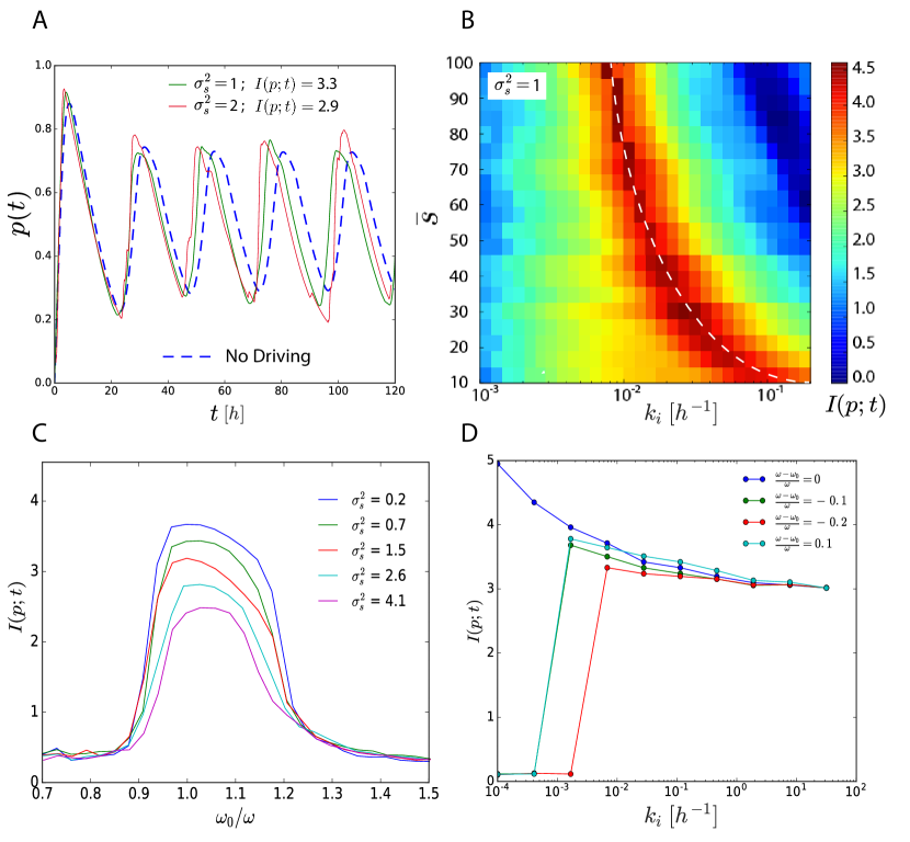
Figure S3: The deterministic coupled-hexamer model. (A) Time traces of $p(t)$ in the abence of driving (dashed line) and in the presence of driving (solid lines), for two different values of the input-noise strength $\sigma^{2}_{s}$; the corresponding values of the mutual information $I(p;t)$ are also shown. In the absence of driving, the system exhibits stable, limit-cycle oscillations. (B) The mutual information $I(p;t)$ as a function of $\bar{s}$ and $k_{i}=k_{1}=\dots=k_{5}$, for $\sigma^{2}_{s}=1$; $k_{\rm b}=0.1875/{\rm h}$ is kept constant while $k_{\rm ps}$ is scaled with the same factor as $k_{i}$. While the intrinsic frequency $\omega_{0}$ is mainly determined by the product $k_{i}\bar{s}$ (the average phosphorylation rate, see Eq. S3), the coupling strength is set by $k_{i}$. Superimposed the white-dashed line along which $k_{i}\bar{s}$ and hence the intrinsic frequency $\omega_{0}$ is constant and equal to the driving frequency $\omega_{0}=\omega=2\pi/24\,{\rm h^{-1}}$. Clearly, the mutual information decreases rapidly as the intrinsic frequency is altered significantly away from the driving frequency $\omega$, as shown more clearly in panel C. Along the (dashed white) line of constant intrinsic frequency, the mutual information decreases as the coupling is increased; this is more clearly illustrated in panel D. (C) The mutual information $I(p;t)$ as a function of the intrinsic frequency $\omega_{0}$, which was varied by scaling all phosphorylation rates $\{k_{\rm ps},k_{i},k_{\rm b}\}$ by a factor $q$, while keeping $\bar{s}=2$. It is seen that there exists an optimal (de)phosphorylation rate that maximizes $I(p;t)$, which weakly depends on $\sigma^{2}_{s}$. It corresponds to an intrinsic period $T_{0}=25.1{\rm h}$ of the free-running clock. (D) The mutual information as a function of $k_{i}$ for different detuning strengths $(\omega-\omega_{0})/\omega$, all for $\sigma^{2}_{s}=1$; $k_{\rm ps}$ is scaled by the same factor as $k_{i}$; $k_{\rm b}=0.1875/{\rm h}$ is kept constant and $\bar{s}$ is changed such that $k_{i}\bar{s}$ and hence the intrinsic frequency $\omega_{0}$ remains constant along each curve. It is seen that for zero detuning, $\omega_{0}=\omega$ (corresponding also to the white dashed line in panel B), the mutual information increases continuously as the coupling strength is decreased; this is because decreasing the coupling makes it possible to minimize input-noise propagation. However, for finite detuning, the mutual information first rises as $k_{i}$ is lowered (because that minimizes input-noise propagation), but then suddenly drops to zero when the system leaves the Arnold tongue: for non-zero detuning, a minimal coupling is necessary to phase-lock the system to the driving signal Monti:2018hs . The noise correlation time $\tau_{c}=0.5{\rm h}$.

Model Since computing the mutual information accurately requires very long simulations, we sought to develop a minimal version of the PPC model presented in VanZon2007 ; Zwicker2010 ; Paijmans:2016fd , which can describe a wealth of data including the concentration dependence of the self-sustained oscillations and the coupling to ATP/ADP VanZon2007 ; Paijmans:2016fd ; Paijmans:2017gp . This model is deterministic and described by the following chemical rate equations:

$$\dot{c}_{0}= k_{\rm s}\tilde{c}_{0}-s(t)c_{0}\left[k_{0}\frac{A}{A+K_{0}}+k_{\rm ps}\frac{K_{0}}{A+K_{0}}\right]$$ (S14)

$$\dot{c}_{i}= s(t)c_{i-1}\left[k_{i-1}\frac{A}{A+K_{i-1}}+k_{\rm ps}\frac{K_{i-1}}{A+K_{i-1}}\right]$$

$$-s(t)c_{i}\left[k_{i}\frac{A}{A+K_{i}}+k_{\rm ps}\frac{K_{i}}{A+K_{i}}\right]i\in(1,\dots,5)$$ (S15)

$$\dot{c}_{6}= s(t)c_{5}\left[k_{5}\frac{A}{A+K_{5}}+k_{\rm ps}\frac{K_{5}}{A+K_{5}}\right]-k_{\rm s}c_{6}$$ (S16)

$$\dot{\tilde{c}}_{6}= k_{\rm s}c_{6}-k_{\rm b}\tilde{c}_{6}$$ (S17)

$$\dot{\tilde{c}}_{i}= k_{\rm b}(\tilde{c}_{i+1}-\tilde{c}_{i})\hskip 28.45274pti\in(1,\dots,5)$$ (S18)

$$\dot{\tilde{c}}_{0}= k_{\rm b}\tilde{c}_{1}-k_{\rm s}\tilde{c}_{0}$$ (S19)

$$A= A_{\rm T}-\sum_{j=0}^{5}c_{j}\frac{A}{A+K_{j}}-\sum_{j=0}^{6}b_{j}\tilde{c}_{j}\frac{A^{b_{j}}}{A^{b_{j}}+\tilde{K}_{j}^{b_{j}}}$$ (S20)

Here, $c_{i}$ and $\tilde{c}_{i}$ are the concentrations of active and inactive $i$-fold phosphorylated KaiC, $A$ is the concentration of free KaiA. The rates $k_{i}$ are the rates of KaiA-stimulated phosphorylation of active KaiC and $k_{\rm ps}$ is the spontaneous phosphorylation rate of active KaiC when KaiA is not bound. Please note that both rates are multiplied by the input signal $s(t)$, since both rates depend on the ATP/ADP ratio Paijmans:2017gx . The dephosphorylation rate $k_{\rm b}$ is independent of the ATP/ADP ratio Lin2014 ; Paijmans:2017gx and hence $k_{\rm b}$ is not multiplied with $s(t)$. As in the UHM, $k_{\rm s}$ is the conformational switching rate. The last equation, Eq. S20, gives the concentration $A$ of free KaiA under the quasi-equilibrium assumption of rapid KaiA (un)binding by active KaiC with affinity $K_{i}$ (second term right-hand side) and rapid binding of KaiA by inactive KaiC, where each $i$-fold phosphorylated inactive KaiC hexamer can bind $b_{i}$ KaiA dimers (last term right-hand side Eq. S20). The mechanism of differential affinity is implemented via two ingredients: 1) the dissociation constant of KaiA binding to active KaiC, $K_{i}$, depends on the phosphorylation level $i$, with less phosphorylated KaiC having a higher binding affinity: $K_{i}<K_{i+1}$ VanZon2007 ; Lin2014 ; Paijmans:2017gx ; 2) inactive KaiC can strongly bind and sequester KaiA VanZon2007 ; Lin2014 ; Paijmans:2017gx ; this is modeled by the last term in Eq. S20.

Autonomous oscillations Fig. S3A shows a time trace of $p(t)$ (Eq. S12) for both a driven and a non-driven coupled-hexamer model. Clearly, in contrast to the push-pull network and the uncoupled-hexamer model, this system exhibits free running simulations. Note also that the autonomous oscillations are slightly asymmetric as observed experimentally, and as shown also by the detailed models on which this minimal model is based VanZon2007 ; Zwicker2010 . Lastly, while the driving signal is sinusoidal, the output signal of the driven system remains non-sinusoidal. This is because this system is non-linear; this behavior is indeed in marked contrast to the behavior seen for the linear UHM (see Fig. S2) and that of the PPN (Fig. S1) which operates in the linear regime. The slight asymmetry in the oscillations also explains why in the regime of very low noise, this system has a slightly lower mutual information than that of push-pull network or the uncoupled-hexamer model, as seen in Fig. 1 of the main text.

Setting the parameters
Free-running oscillator We first set the parameters to get autonomous oscillations, keeping $s(t)=\bar{s}=2$. These parameters were inspired by the parameters of the model upon which the current model is built VanZon2007 . Specifically, the KaiA binding affinity of active KaiC, given by $K_{i}$, was chosen such that it obeys differential affinity, $K_{0}<K_{1}<K_{2}<K_{3}<K_{4}<K_{5}$ , as in the PPC model of VanZon2007 ; Zwicker2010 ; Paijmans:2016fd . In addition, in our model, $b_{i}=2$ for $i=1,2,3,4$ and $b_{i}=0$ for $i=0,5,6$, meaning that $i=1-4$ fold phosphorylated inactive KaiC hexamers can each bind two KaiA dimers with strong affinity $\tilde{K}_{i}=\tilde{K}$. The conformational switching rate $k_{\rm s}$ was set to be higher than all the (de)phosphorylation rates, $k_{\rm s}>>\{k_{i},k_{\rm ps},k_{b}\}$ and the values of $k_{i},k_{\rm ps},k_{\rm b}$ were, again apart from a scaling factor to set the optimal intrinsic frequency as described below, identical to those of the PPC model of VanZon2007 ; Lin2014 ; Paijmans:2016fd . These parameter values allowed for robust free-running oscillations (see Fig. S3A) in near quantitative agreement with the oscillations of the more detailed PPC model of VanZon2007 ; Lin2014 ; Paijmans:2016fd .

Driven oscillator: Optimal intrinsic frequency We then studied the driven system. We computed the mutual information $I(p;t)$ as a function of the mean signal $\bar{s}$ and the phosphorylation rates $k_{i}=k_{1}=\dots=k_{5}$, see Fig. S3B. While the intrinsic frequency is primarily determined by the mean phosphorylation rate $k_{i}\bar{s}$, as illustrated by the dashed-white line of constant intrinsic frequency $\omega_{0}$, the coupling strength is (for a given mean $k_{i}\bar{s}$) set by the amplitude $k_{i}$ (see Eq. S3). Panel B shows that the mutual information changes markedly in the direction perpendicular to the white line, indicating that $I(p;t)$ strongly depends on $\omega_{0}$. To illustrate this further, we varied the intrinsic frequency $\omega_{0}$ of the autonomous oscillations by varying all (de) phosphorylation rates $\{k_{i},k_{\rm ps},k_{b}\}$ by a constant factor and computed the mutual information $I(p;t)$ as a function of this factor and hence $\omega_{0}$. The result is shown in Fig. S3C. Clearly, as for the uncoupled-hexamer model, there exists an optimal intrinsic frequency $\omega_{0}^{\rm opt}$ that maximizes $I(p;t)$. The optimal intrinic frequency depends on the input-noise strength: for low input noise, $\omega_{0}^{\rm opt}<\omega$, but then $\omega_{0}^{\rm opt}$ increases with $\sigma^{2}_{s}$ to become similar to $\omega$ in the high noise regime. We also see, however, that the dependence of $\omega_{0}^{\rm opt}$ on $\sigma^{2}_{s}$ is rather weak (Fig. S3B). We therefore kept the parameters in the simulations corresponding to Fig. 2 of the main text, constant.

Driven oscillator: mutual information increases with decreasing coupling strength as long as the system remains inside the Arnold tongue. Along the white dashed line of panel B (corresponding to the blue line in panel D), $\omega_{0}=\omega$, and the mutual information $I(p;t)$ decreases as the coupling strength $k_{i}$ is increased. Indeed, when there is no detuning ($\omega_{0}=\omega$) and no internal noise, $I(p;t)$ is maximized when the coupling strength goes to zero. This can be understood by noting that a) the limit-cycle oscillator has, in stark contrast to the push-pull network and the uncoupled-hexamer system, an intrinsic robust amplitude, which does not rely on driving by the input signal; b) decreasing the coupling reduces the propagation of the input fluctuations. In section SII.5 we prove analytically that concerning the robustness to input noise: a) the optimal regime is that of weak coupling; b) in this regime, systems based on a limit-cycle attractor, such as the CHM, are superior to those based on a fixed-point attractor, such as the PPN and the UHM.

Driven oscillator: With non-zero detuning, coupling is necessary to keep the system inside the Arnold tongue. Importantly, there will always be a finite amount of internal noise. In addition, the intrisic period will never be exacly $24{\rm h}$. In both cases, coupling is essential to keep the system in phase with the driving signal. In the next section we discuss the role of internal noise, but in panel D of Fig. S3 we show for the deterministic CHM the importance of coupling when there is a finite amount of detuning $(\omega-\omega_{0})/\omega$. Clearly, for non-zero detuning, the mutual information first rises as the coupling strength is decreased (because that minimizes input-noise propagation), but then suddenly drops as the system moves out of the Arnod tongue: when the intrinsic period does not match the period of the driving signal, a minimal coupling is essential to firmly lock the oscillations to the input signal (keeping the system inside the Arnold tongue); indeed, as panel D shows, the required coupling strength increases with the amount of detuning Monti:2018hs .

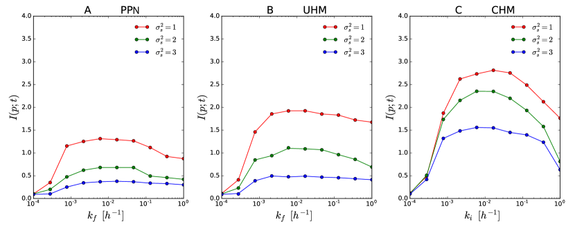
Figure S4: Optimal coupling strength in the three different computational models in the presence of input noise and internal noise. To isolate the role of internal noise, the detuning for both the uncoupled and coupled hexamer model was set to zero. Shown is the mutual information $I(p;t)$ as a function of the coupling strength $k_{\rm f}$ and $k_{i}$ for different input-noise levels $\sigma^{2}_{s}$, for: (A) The push-pull network (PPN); (B) Uncoupled hexamer model (UHM); (C) Coupled hexamer model (CHM). In all three models, the internal noise was kept constant, by keeping the copy number of the central clock protein at $N=1000$; this number is comparable to the number of KaiC hexamers as measured for the cyanobacterium S. elongatus in vivo Kitayama:2003un . The results were obtained by performing stochastic Gillespie simulations. For the push-pull network (panel A), the de-phosphorylation rate $k_{\rm b}$ is set to the optimal one as predicted by Eq. S45. The stochastic models of the UHM and CHM are based of the PPC of Zwicker2010 . It is seen that for all three models there exists an optimal coupling constant that maximizes the mutual information. For the PPN and UHM, the optimum is broad: for low coupling, the internal noise dominates, and coupling is necessary to lift the signal (amplitude oscillations) above the internal noise; for higher coupling, the input noise dominates over the internal noise, and the signal-to-noise ratio (and hence the mutual information) becomes independent of the coupling strength; for even larger coupling strength, the mutual information goes down because of signal distortion. For the CHM, the optimum is sharper, arising from a pronounced trade-off between minimizing input-noise propagation and maximizing internal-noise suppression. Parameters: PPN: $k_{\rm b}=0.3/{\rm h}$; UHM: $\bar{s}$ is scaled with $k_{\rm f}$ such that $k_{\rm f}\bar{s}=k_{\rm b}=0.5/{\rm h}$ and $\omega_{0}=\omega$ (see Eq. S13); CHM: $\bar{s}$ is scaled with $k_{i}$ such that $\omega_{0}=\omega$; $k_{\rm ps}$ is scaled with $k_{i}$; $k_{\rm b}=0.1875/{\rm h}$ is kept constant; other parameters, see S1.

Setting the coupling strength and the other parameters The fact that the mutual information depends on the amount of detuning (Fig. S3D) and also internal noise, as shown in the next section (Fig. S4), raises the question what is the natural procedure to set its value. We have decided to set the relative coupling strength to a value that is comparable to the coupling strength of the PPC of S. elongatus. Specifically, Fig. 3B of Phong et al. Phong:2013fr shows that the kinase rate of the CII domain increases from $0.1/{\rm h}$ at an ATP fraction of 25% to $0.42/{\rm h}$ at an ATP fraction of 100%. Assuming the ATP fraction oscillates between these levels inside the cell Rust2011 , the amplitude over the mean of the oscillations of the kinase rate is around $0.6$. This should be compared to $k_{i}/(k_{i}\bar{s})=1/\bar{s}$ in our model (see Eq. S3). With $\bar{s}=2$, the coupling strength is indeed comparable to that of the PPC of S. elongatus. We thus kept $\bar{s}=2$ fixed and then optimized over the intrinsic frequency by scaling the (de)phosphorylation rates $k_{i},k_{\rm ps},k_{\rm b}$, as shown in Fig. S3C. This yielded $\omega_{0}^{\rm opt}=0.96\omega$, corresponding to an intrinsic period $T_{0}=25.1{\rm h}$. Table S1 gives an overview of all the parameters. Finally, we emphasize that the chosen coupling strength is a conservative estimate: if the ATP fraction oscillates from 0.2 to 0.6 inside the cell Rust2011 , then the in vivo coupling strength will be lower; as panel D shows, the performance of the CHM, regarding robustness to input noise, will then even be higher. In fact, as Fig. S5A shows, the optimal coupling strength that maximizes the mutual information for the CHM in the presence of both detuning and internal noise at biologically relevant strengths, is even lower than that corresponding to Fig. 2 of the main text. In comparing the CHM against the UHM and PPN, we thus consider a “worst-case” scenario for the CHM. Indeed, even for this scenario, the CHM is much more robust to input noise than the PPN and UHM, as Fig. 2 of the main text shows.

SI.5 Robustness to internal noise

The computational models of the readout systems considered in the main text and above are deterministic; only the input signal is stochastic. In this section, we address the question how robust the results on our computational models are to the presence of internal noise that arises from the inherent stochasticity of chemical reactions. To isolate the effect of internal noise, we first zoom in on the interplay between internal and input noise in the absence of any detuning for the UHM and CHM (Fig. S4), and then we study the biologically relevant regime with a finite amount of detuning (Fig. S5). Fig. S4 shows that in the presence of both sources of noise, all computational models exhibit an optimal coupling strength that maximizes information transmission. Fig. S5 then demonstrates that in the biologically relevant regime, at least for cyanobacteria: 1) the optimal coupling is weak because the input noise dominates over the internal noise; 2) the coupled-hexamer model is more robust to input noise than the push-pull network and the uncoupled-hexamer model. We elucidate these results using our analytical models in sections SII.5 and SII.6.

Stochastic simulations To investigate the role of internal noise, we have performed stochastic Gillespie simulations Gillespie:1977dc of all three computational models. These simulations take into account the inherent stochasticity of the chemical reactions, yet do assume that the system remains well-stirred at all times. We keep the magnitude of the internal noise fixed by keeping the copy number $N$ of the central clock component, $X$ in the PPN and the KaiC hexamer in the UHM and CHM, constant at $N=1000$; this number is comparable to the number of KaiC hexamers in the cyanobacterium S. elongatus Kitayama:2003un . The stochastic model of the PPN and the UHM are the stochastic versions of the deterministic models studied above and in the main text, taking into account the stochastic phosphorylation and dephosphorylation of $X$ and KaiC, respectively. For the stochastic model of the CHM, we have adopted the stochastic PPC model, including its parameter values Zwicker2010 ; here, KaiA and KaiB binding is modeled explicitly, but since these reactions are much faster than the (de)phosphorylation reactions, this is not important—to an excellent approximation, this model is the stochastic equivalent of the deterministic CHM studied in the main text and above.

SI.5.1 The interplay between input and internal noise with no detuning

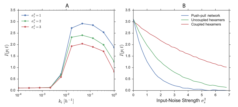
Figure S5: Comparing the coupled-hexamer model (CHM) with biologically relevant levels of internal noise and detuning against the optimal push-pull network (PPN) and optimal uncoupled-hexamer model (UHM). For all models, the internal noise was kept constant by keeping the copy number of the central clock component at $N=1000$, which is comparable to the number of KaiC hexamers as measured in vivo for the cyanobacterium S. elongatus Kitayama:2003un . For the CHM, the amount of detuning was set to $(\omega-\omega_{0})/\omega=-0.1$, which corresponds to that measured for the reconstitued PPC of S. elongatus Nakajima2005 . Weather data Gu:2001vh indicates that the average input noise strength is $\sigma^{2}_{s}\approx 1-2$, but since there will be variations in the fluctuations in the light intensity from day to day, we also consider higher input noise strengths (see section SI.1) (A) The mutual information $I(p;t)$ of the CHM as a function of coupling strength $k_{i}$ for 3 different input-noise strengths; $k_{\rm b}=0.1875/{\rm h}$ and $k_{\rm ps}$ is scaled by the same factor as $k_{i}$; $\bar{s}$ is changed such that the intrinsic frequency and hence amount of detuning is constant along each curve. It is seen that the mutual information is initially low but then sharply rises with $k_{i}$ as the system enters the Arnold tongue where the CHM becomes firmly locked to the driving signal (compare with Fig. S3D). When the coupling strength is raised further, the mutual information goes through a maximum, which arises from a trade-off between minimizing input-noise propagation and maximizing internal-noise suppression. Importantly, the optimal coupling strength is low, indicating that the input noise dominates over the internal noise. Please also note that the maximum is broader than that in Fig. S3D, due to the internal noise. (B) The mutual information $I(p;t)$ as a function of input-noise strength for the three different computational models. For the CHM, all parameters (but most notably $k_{i},k_{\rm ps},k_{\rm b}$) have the baseline parameter values corresponding to Fig. 2 of the main text and shown in Table S1, except $\bar{s}$, which was changed such that the detuning is $(\omega-\omega_{0})/\omega=-0.1$. For the UHM and PPN, all parameters (including $\bar{s}$) have the baseline parameter values corresponding to Fig. 2 and shown in table S1; these parameter values maximize the mutual information in the absence of internal noise (see Fig. S1C and Fig. S2C). The figure shows that the principal finding of our manuscript, shown in Fig. 2 of the main text, is robust to the presence of internal noise: in the limit of low input-noise, the mutual information is similar for all systems. Yet, in the regime of high input noise, the CHM has the highest mutual information. The results were obtained by performing stochastic Gillespie simulations Gillespie:1977dc .

In the previous sections, we have seen that for the deterministic push-pull network and the deterministic uncoupled-hexamer model, the mutual information is essentially independent of the coupling strength in the weak-coupling regime, because increasing the coupling strength increases both the amplitude of the output (the gain) and the amplification of the input noise, leaving the signal-to-noise ratio unchanged. In contrast, for the CHM, when the intrinsic clock period is not equal to that of the driving signal, a minimal amount of coupling is necessary to phase-lock the clock to the driving and put the system inside the Arnold tongue (Fig. S3D). Yet, once the system is inside the Arnold tongue the coupling should be as low as possible to minimize input-noise propagation.

However, for all three systems, we expect that in the presence of internal noise there is a positive effect of increasing the coupling strength, although, interestingly, the origin of the effect is different for the three respective systems: for the fixed-point attractors (PPN and UHM), increasing the coupling helps to raise the the amplitude of the oscillations (the signal) above the internal noise, while for the limit-cycle attractor (CHM) increasing the coupling increases the restoring force that contains the effect of the internal noise. Section SII.6 discusses these effects in more detail.

In Fig. S4 we show for all three models separately, the mutual information $I(p;t)$ as a function of the coupling strength, for different strengths of the input noise, keeping the internal noise constant. We see that in all cases there exists an optimal coupling strength that maximizes the mutual information, as predicted by the analytical models discussed in section SII.6. For the fixed-point attractors, the PPN and the UHM, the optimum is broad: a minimal coupling is required to raise the signal above the internal noise, but for larger coupling strengths the effect of the input noise, which increases with the coupling, dominates over the internal noise, and in this regime the signal-to-noise ratio is essentially constant; for even larger coupling, however, the signal will saturate (because $p(t)$ is bounded by zero and unity), and this will lead to non-sinusoidal oscillations, causing the mutual information to go down. For the limit-cycle attractor (the CHM), the optimum is more pronounced, arising from a sharp trade-off between minimizing input-noise propagation (which favors weak coupling) and maximizing internal noise suppression (which favors strong coupling). Indeed, panel C shows that the optimal coupling strength decreases as the input noise is increased, precisely as this argument predicts.

SI.5.2 Interplay between internal and input noise with detuning

In vivo, not only a finite amount of internal noise is inevitable, but also a non-zero amount of detuning. In this section, we compare the three computational models in the presence of both internal noise and detuning at biologically relevant levels.

Panel A of Fig. S5 shows for the CHM the mutual information $I(p;t)$ as a function of the coupling strength $k_{i}$, for three different input-noise levels, in the presence of internal noise and detuning at biologicallly relevant levels. As above, the internal noise is set by the copy number $N=1000$ corresponding to the number of KaiC hexamers in S. elongatus Kitayama:2003un , while the detuning is $(\omega-\omega_{0})/\omega=-0.1$ as measured experimentally for the reconstituted PPC of S. elongatus Nakajima2005 . Panel A exhibits a mixture of the behavior of Fig. S3D corresponding to the CHM with finite detuning and no internal noise, and that of Fig. S4C corresponding to no detuning but with internal noise present: to increase the mutual information, the coupling strength first has to rise to bring the system inside the Arnold tongue (compare with Fig. S3D). Yet once inside the Arnold tongue, $I(p;t)$ features an optimum arising from the interplay between minimizing input-noise propagation and maximizing internal noise suppression. We also see that the optimal coupling strength, for all input-noise levels, is lower than that of the CHM of Fig. 2 of the main text; with such a weaker coupling, the robustness of the CHM to input noise would be even higher.

In Fig. S5 we compare the performance of the three computational models as a function of input-noise strength, in the presence of both internal noise and detuning at biologically relevant levels. Clearly, as observed for the deterministic systems corresponding to Fig. 2 of the main text, for low input noise, the performance of the three systems is very similar. Yet, for high input noise, the CHM is far superior. We thus conclude that the principal result of the main text, namely that a limit-cycle oscillator such as the CHM is more robust to input noise than a damped oscillator such as the PPN or UHM, is robust to the presence of internal noise.

We can understand this result by noting that in the presence of biologically relevant amounts of internal noise and input noise, the optimal coupling is weak because the input noise dominates over the internal noise. In fact, experiments have revealed that the clock of S. elongatus has a strong temporal stability with a correlation time of several months, indicating that the internal noise is indeed small Mihalcescu:2004ch . As we prove analytically in SII.5, in the input-noise dominated regime a limit-cycle oscillator, such as the CHM, is generically more resilient to input noise than a system with a fixed point attractor, such as the PPN and UHM. Reducing the coupling minimizes the amplification of the input noise in all systems, but only the limit-cycle oscillator (CHM) can still sustain robust large-amplitude oscillations in this regime.

For larger internal noise strengths than that considered here, thus outside the biological realm, it might be beneficial to increase the coupling further. Strong coupling makes it possible to exploit the fact that the output $p(t)$ is naturally bounded between zero and unity; the noise can thus be tamed by continually pushing $p(t)$ against either zero and unity. This generates, however, strongly non-sinusoidal, square-wave like oscillations, which are not experimentally observed Rust2007 . We thus leave the regime of strong coupling for future work.

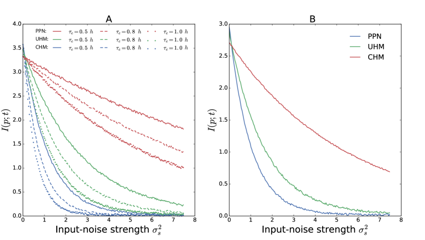
Figure S6: Robustness of the pricipal resut of our paper, Fig. 2 of the main text, to the shape and correlation time of the input signal. (A) Robustness to correlation time of the input noise. It is seen that increasing the correlation time $\tau_{c}$ of the input noise lowers the mutual information $I(p;t)$. This is because a higher correlation time impedes noise averaging Paulsson:2004dh ; TanaseNicola:2006bh ; Govern:2014ez . Yet, for all values of $\tau_{c}$ the result of Fig. 2 of the main text is recapitulated: when the input-noise strength $\sigma^{2}_{s}$ is low, all readout systems are equally accurate; yet, in the high noise regime, the coupled-hexamer model is superior. (B) Robustness to the shape of the input signal. Here, the input is a truncated sinusoidal signal so that during the night $s(t)=0$, while during the day $s(t)$ is a half sinusoid (see Eq. S21). As expected, shutting off the driving during the night lowers the mutual information (compare with panel A). More strikingly, in the regime of low input noise, all readout systems are again equally informative on time. Clearly, the push-pull network and uncoupled-hexamer model do not need to be driven constantly; it is sufficient that the light drives the phosphorylation of the readout proteins during the day, so that they can dephosphorylate spontaneously during the night. In the regime of high input-noise, the coupled-hexamer system is again optimal. In panel B, the noise correlation time $\tau_{c}=0.5{\rm h}$. Other parameters are in Table S1.

SI.6 Robustness to shape of input signal

We have tested the robustness of our principal result, shown in Fig. 2 of the main text, by varying a number of key parameters. We first varied the correlation time $\tau_{c}$ of the noise, see Fig. S6A. Clearly, the main result is robust to variations in the value of $\tau_{c}$: in the limit of small input-noise $\sigma^{2}_{s}$ all three time-keeping systems are equally accurate, while for large input noise the bonafide clock is far superior. We have also varied the nature of the input signal. Specifically, instead of a sinusoidal signal we have also studied a truncated sinusoidal signal $s(t)$, which drops to zero for 12 hours during the night but is a half-sinusoid for 12 hours during the day:

$$s(t)=h(t)\left\{\sin(\omega t)+\eta_{s}(t)\right\},$$ (S21)

where $h(t)=0$ for $0<t<12$ and $h(t)=1$ for $12<t<24$. The result is shown in Fig. S6B. It is seen that the principal result of Fig. 2 of the main text is also insensitive to the precise choice of the input signal.

The robustness of our principal observations indicate they are universal and should be observable in minimal generic models. These are described in the next sections.

SI.7 Computing the mutual information

The mutual information is given by

$$I(p;t)=\int_{0}^{t}dp\int_{0}^{T}dtP(p,t)\log_{2}\frac{P(p,t)}{P(p)P(t)},$$ (S22)

where $P(p,t)$ is the joint probability distribution of the phosphorylation level $p$ and time $t$ and $P(p)$ and $P(t)$ are the marginal probability distribution functions of $p$ and $t$, respectively. When $p$ and $t$ are statistically independent, $P(p,t)=P(p)P(t)$ and the mutual information $I(p;t)$ is indeed zero. More generally, $2^{I(p;t)}$ corresponds the number of time points $t$ that can be inferred uniquely from the phosphorylation level $p$; it thus corresponds to the number of distinguishable mappings between $t$ and $p$ Walczak:1324157 . The mutual information depends on the entropy of the input distribution $H(t)$ and the accuracy of signal transmission, which can be seen by rewriting Eq. S22 as

$$I(p;t)=H(t)-\langle H(t|p)\rangle_{p},$$ (S23)

where

$$H(t)=-\int_{0}^{T}dtP(t)\log_{2}P(t)$$ (S24)

is the entropy of the input distribution $P(t)=1/T$ and

$$\langle H(t|p)\rangle_{p}=-\int_{0}^{1}dpP(p)\int_{0}^{T}dtP(t|p)\log_{2}P(t|p)$$ (S25)

is the average of the entropy of the conditional distribution of $t$ given $p$, $P(t|p)$. The input entropy $H(t)$ quantifies the a priori uncertainty on the input, while $\langle H(t|p)\rangle_{p}$ quantifies the uncertainty on the input $t$ after the output $p$ has been measured. Eq. S26 shows that the mutual information can be interpreted as the reduction in the uncertainty on the input $t$, by measuring the output $p$. The conditional entropy $\langle H(t|p)\rangle_{p}$ depends on the reliability of signal transmission, and goes to zero when the signal is transduced perfectly. Indeed, since the input distribution $P(t)$ is continuous, the mutual information diverges when there is no input noise (and no internal noise). The highest mutual information reported in Fig. 2 of the main text thus corresponds to the smallest input-noise level studied. For a more detailed discussion of the mutual information, we refer to Walczak:1324157 .

The mutual information is symmetric with respect to its arguments, and Eq. S22 can also be rewritten as

$$I(p;t)=H(p)-\langle H(p|t)\rangle_{t}.$$ (S26)

where

$$H(p)=-\int_{0}^{1}dpP(p)\log_{2}P(p)$$ (S27)

is the entropy of the output distribution $P(p)$ and

$$\langle H(p|t)\rangle_{t}=-\frac{1}{T}\int_{0}^{T}dt\int_{0}^{1}dpP(p|t)\log_{2}P(p|t)$$ (S28)

is the average of the conditional entropy of $P(p|t)$, with $P(p|t)$ the conditional distribution of $p$ given $t$. We have used this form to compute $I(p;t)$. In numerically computing the mutual information, we have verified that the results are independent of the bin size of the distribution of $p$, following the approach of Cheong:2011jp .

SII Analytical models

SII.1 Push-pull network

The equation for the push-pull network is

$$\dot{x}_{p} =k_{\rm f}s(t)(x_{T}-x_{p}(t))-k_{\rm b}x_{p}$$ (S29)

$$\simeq k_{\rm f}s(t)x_{T}-k_{\rm b}x_{p},$$ (S30)

where in the last equation we have assumed that $x_{T}\gg x_{p}$, which is the case when $k_{\rm f}s(t)\ll k_{\rm b}$. In this regime, the push-pull network operates in the linear regime, leading to sinusoidal oscillations, which tend to enhance information transmission Monti:2016bp . In what follows, we write, to facilitate comparison with other studies on noise transmission Tostevin:2010bo ; Monti:2016bp $\rho\equiv k_{\rm f}x_{\rm T}$, $\mu=k_{\rm b}$ and, for notational convenience, $x_{p}=x$. We thus study

$$\dot{x}=\rho s(t)-\mu x(t).$$ (S31)

The equation can be solved analytically to yield

$$x(t)=\int_{-\infty}^{t}dt^{\prime}\chi(t-t^{\prime})s(t),$$ (S32)

with $\chi(t-t^{\prime})=\rho e^{-\mu(t-t^{\prime})}$. With the input signal given by

$$s(t)=\sin(\omega t)+\bar{s}+\eta_{s}(t),$$ (S33)

the output is

$$x(t)=A\sin(\omega t-\phi)+\bar{x}+\eta_{x}(t)$$ (S34)

where the amplitude is

$$A=\frac{\rho}{\sqrt{\mu^{2}+\omega^{2}}},$$ (S35)

the phase difference of the output with the input is

$$\phi=\arctan(\omega/\mu),$$ (S36)

the mean is

$$\bar{x}=\rho\bar{s}/\mu$$ (S37)

and the noise is

$$\eta_{x}=\rho\int_{-\infty}^{t}dt^{\prime}e^{-\mu(t-t^{\prime})}\eta_{s}(t^{\prime}).$$ (S38)

The variance of the output, assuming the system is in steady state, is then

$$\sigma^{2}_{x} =\langle(x(0)-\bar{x}(0))^{2}\rangle$$ (S39)

$$=\rho^{2}\int_{-\infty}^{0}\int_{-\infty}^{0}dtdt^{\prime}e^{\mu(t+t^{\prime})}\langle\eta_{s}(t)\eta_{s}(t^{\prime})\rangle.$$ (S40)

Assuming that the input noise has variance $\sigma^{2}_{s}$ and decays exponentially with correlation time $\tau_{c}=\lambda^{-1}$, meaning that $\langle\eta_{s}(t)\eta_{s}(t^{\prime})\rangle=\sigma^{2}_{s}e^{-\lambda|t-t^{\prime}|}$, the variance of the output is

$$\sigma^{2}_{x} =\rho^{2}\sigma^{2}_{s}\left[\int_{-\infty}^{0}\int_{-\infty}^{t}dtdt^{\prime}e^{\mu(t+t^{\prime})}e^{-\lambda(t-t^{\prime})}+\right.$$ (S41)

$$\left.\int_{-\infty}^{0}\int_{t}^{0}dtdt^{\prime}e^{\mu(t+t^{\prime})}e^{+\lambda(t-t^{\prime})}\right]$$ (S42)

$$=g^{2}\frac{\mu}{\mu+\lambda}\sigma^{2}_{s},$$ (S43)

with the gain given by $g\equiv\rho/\mu$.

The signal-to-noise ratio $A/\sigma_{x}$ is then

$$\frac{A}{\sigma_{x}}=\sqrt{\frac{\mu(\mu+\lambda)}{\mu^{2}+\omega^{2}}}\frac{1}{\sigma_{s}},$$ (S44)

which has a maximum at the optimal relaxation rate Monti:2016bp

$$\mu^{\rm opt} =\frac{\omega^{2}}{\lambda}\left(1+\sqrt{1+\left(\lambda/\omega\right)^{2}}\right).$$ (S45)

This optimum arises from a trade-off between the amplitude, which increases as $\mu$ increases, and input-noise averaging, which improves as $\mu$ decreases. Another point to note is that the optimal signal-to-noise ratio does not depend on $\rho=k_{\rm f}x_{\rm T}$, and hence not on $k_{\rm f}$ and $x_{\rm T}$: while increasing $\rho$ increases the amplitude of the signal, it also amplifies the noise in the input signal. Increasing the gain $\rho$ (via $x_{\rm T}$ and/or $k_{\rm f}$) only helps in the presence of intrinsic noise, because increasing the amplitude of the signal helps to raise the signal above the intrinsic noise Monti:2016bp , as discussed in sections SI.5 and SII.6. However, in the deterministic models considered in this study, the intrinsic noise is zero.

SII.2 The harmonic oscillator and the uncoupled-hexamer model

The uncoupled-hexamer model (UHM) is linear. Moreover, because each hexamer has a phosphorylation cycle with a characteristic oscillatino frequency $\omega_{0}$, this system is akin to the harmonic oscillator. Indeed, when not driven, both the UHM and the harmonic oscillator relax in an oscillatory fashion to a stable fixed point. To develop intuition on the behavior of the UHM, we therefore here analyze the behavior of a harmonic oscillator driven by a noisy sinusoidal signal.

The equation of motion of the driven harmonic oscillator is

$$\ddot{x}+\omega^{2}_{0}x+\gamma\dot{x}=\rho s(t),$$ (S46)

where $\omega_{0}$ is the characteristic frequency, $\gamma$ is the friction and $\rho$ describes the strength of the coupling to the input signal $s(t)$. We assume that $s(t)=\sin(\omega t)+\eta_{s}(t)$. We note that while the undriven harmonic oscillator is isomorphic to the undriven UHM, their coupling to the input is different: in the UHM, the hexamers are, motivated by the Kai system Rust2011 ; Pattanayak:2015jm , only coupled to the input during their active phosphorylation phase, while the harmonic oscillator is coupled continuously; moreover, in the harmonic oscillator the noise is additive, while in the UHM the signal multiplies the phosphorylation rate, leading to multiplicative noise. Yet, the behavior of the two models is qualitatively similar, as discussed below.

Solving Eq. S46 in Fourier space yields $\tilde{x}(\omega)=\tilde{\chi}(\omega)\tilde{s}(\omega)$, with

$$\tilde{\chi}(\omega)=\frac{\rho}{\omega_{0}^{2}-\omega^{2}-i\omega\gamma}.$$ (S47)

Hence, the time evolution of $x(t)$ is

$$x(t) =\frac{1}{2\pi}\int_{-\infty}^{\infty}d\omega e^{-i\omega t}\tilde{\chi}(\omega)s(\omega)$$ (S48)

$$=\frac{\rho}{2\pi}\int_{-\infty}^{\infty}d\omega\int_{-\infty}^{\infty}dt^{\prime}\frac{e^{i\omega(t^{\prime}-t)}s(t^{\prime})}{\omega^{2}_{0}-\omega^{2}-i\omega\gamma}.$$ (S49)

We do the integral over $\omega$ first. The integrand has poles at

$$\omega=\frac{-i\gamma}{2}\pm\sqrt{\omega_{0}^{2}-\frac{\gamma^{2}}{4}}\equiv\frac{-i\gamma}{2}\pm\omega_{1}.$$ (S50)

This yields

$$x(t) =\frac{\rho}{2\pi}\int_{-\infty}^{\infty}s(t^{\prime})\theta(t-t^{\prime})(2\pi i)\times$$ (S51)

$$\left[\frac{e^{i(-i\frac{\gamma}{2}+\omega_{1})(t^{\prime}-t)}}{2\omega_{1}}-\frac{e^{i(-i\frac{\gamma}{2}-\omega_{1})(t^{\prime}-t)}}{2\omega_{1}}\right]$$ (S52)

$$=\frac{\rho}{\omega_{1}}\int_{-\infty}^{t}dt^{\prime}e^{-\frac{\gamma}{2}(t-t^{\prime})}\sin(\omega_{1}(t-t^{\prime}))s(t^{\prime}).$$ (S53)

With $s(t)=\sin(\omega t)$, this yields

$$x(t) =\frac{-\gamma\omega\cos[\omega t]+(-\omega^{2}+\omega_{0}^{2})\sin[\omega t]}{\gamma^{2}\omega^{2}+(\omega^{2}-\omega_{0}^{2})^{2}}$$ (S54)

This can also be rewritten as

$$x(t)=A\sin(\omega t+\phi),$$ (S55)

with the amplitude given by

$$A =\frac{\rho}{\sqrt{\gamma^{2}\omega^{2}+(\omega^{2}-\omega_{0}^{2})^{2}}}$$ (S56)

and the phase given by

$$\phi=\arctan\left[\frac{-4\gamma\omega}{\gamma^{2}+4(\omega_{1}^{2}-\omega^{2})}\right].$$ (S57)

Eq. S56 shows that the amplitude increases as the friction decreases and that the amplitude is maximal when the intrinsic frequency equals the driving frequency; in fact, when $\gamma\to 0$ and $\omega_{0}=\omega$, the amplitude diverges.

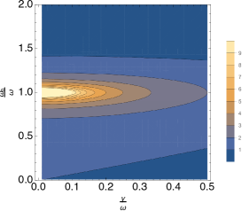
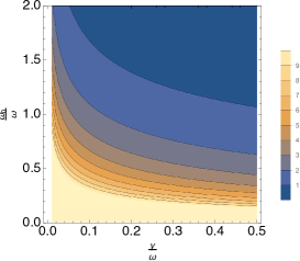
(A)    (B)    (C)

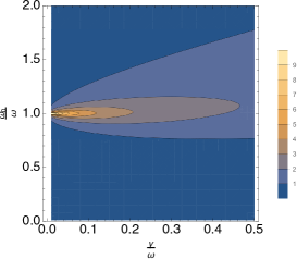
Figure S7: The amplitude (A), standard deviation $\sigma_{x}$ (B), and signal-to-noise ratio $A/\sigma_{x}$ (C) as a function of the the intrinsic frequency $\omega_{0}$ and friction $\gamma$ for the harmonic oscillator. It is seen that the amplitude peaks when $\gamma=0$ and the intrinsic frequency equals the driving frequency, $\omega_{0}=\omega$ (A). The noise peaks at $\gamma=0$ and at $\omega_{0}=0$ (B). Because the amplitude peaks at $\omega_{0}=\omega$, while the noise peaks at $\omega_{0}=0$, there is an optimal intrinsic frequency $\omega_{0}^{\rm opt}>\omega$ that maximizes the signal-to-noise ratio (C). See also Fig. S8.

With an input noise with variance $\sigma^{2}_{s}$ and decay rate $\lambda$, the noise in the output, $\sigma^{2}_{x}=\langle\delta x^{2}(0)\rangle$, is given by

$$\sigma^{2}_{x} =\frac{\rho^{2}}{\omega_{1}^{2}}\int_{-\infty}^{0}dt\int_{-\infty}^{0}dt^{\prime}e^{\frac{\gamma}{2}(t+t^{\prime})}\sin(\omega_{1}t)\sin(\omega_{1}t^{\prime})\langle\eta_{s}(t)\eta_{s}(t^{\prime})\rangle$$ (S58)

$$=\frac{\rho^{2}\sigma^{2}_{s}}{\omega_{1}^{2}}\left[\int_{-\infty}^{0}dt\int_{-\infty}^{t}dt^{\prime}e^{\frac{\gamma}{2}(t+t^{\prime})}\sin(\omega_{1}t)\sin(\omega_{1}t)e^{-\lambda(t-t^{\prime})}\right.$$

$$+\left.\int_{-\infty}^{0}dt\int_{t}^{0}dt^{\prime}e^{\frac{\gamma}{2}(t+t^{\prime})}\sin(\omega_{1}t)\sin(\omega_{1}t^{\prime})e^{-\lambda(t^{\prime}-t)}\right]$$ (S59)

$$=\rho^{2}\sigma^{2}_{s}\frac{16(\gamma+\lambda)}{\gamma[(\gamma+2\lambda)^{2}+4\omega_{1}^{2}](\gamma^{2}+4\omega_{1}^{2})}$$ (S60)

$$=\rho^{2}\sigma^{2}_{s}\frac{(\gamma+\lambda)}{\gamma\omega_{0}^{2}[\lambda(\gamma+\lambda)+\omega_{0}^{2}]}$$ (S61)

This expression shows that the noise diverges for all frequencies when the friction $\gamma\to 0$. It also shows that the noise diverges for $\omega_{0}\to 0$ for all values of $\gamma$, or, conversely, that it goes to zero for $\omega_{0}\to\infty$. This can be understood by imagining a particle with mass $m=1$ in a harmonic potential well with spring constant $k$, giving a resonance frequency $\omega_{0}^{2}=k/m=k$, which is buffeted by stochastic forces: its variance decreases as the spring constant $k$ and intrinsic frequency $\omega_{0}$ increase.

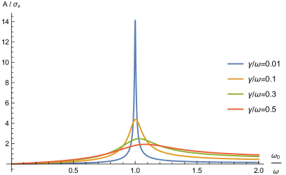
Figure S8: The signal-to-noise $A/\sigma_{x}$ of the harmonic oscillation as a function of $\omega_{0}$ for different values of $\gamma$. Because the amplitude $A$ exhibits a strong maximum at $\omega_{0}=\omega$, the SNR peaks around $\omega_{0}=\omega$. However, the maximum is not precisely at $\omega_{0}=\omega$, because the noise $\sigma_{x}$ peaks at $\omega_{0}=0$ and not at $\omega_{0}=\omega$. Depending on the friction, there thus exists an optimal intrinsic frequency $\omega_{0}^{\rm opt}>\omega$. Note also that when $\omega\neq\omega_{0}$, it is actually beneficial to have friction, $\gamma\neq 0$.

Figs. S7 and S8 show the amplitude $A$, noise $\sigma^{2}_{x}$, and signal-to-noise ratio $A/\sigma_{x}$ for the harmonic oscillator. Clearly, the amplitude is maximal at resonance, diverging when $\gamma\to 0$ (Fig. S7A). The noise is maximal at $\omega_{0}\to 0$, and also diverges for all frequencies when $\gamma\to 0$ (Fig. S7B). However, the amplitude rises more rapidly as $\gamma\to 0$ than the noise does, leading to a global optimum of the signal-to-noise ratio for $\omega_{0}=\omega$ and $\gamma\to 0$ (Fig. S7C). However, biochemical networks have, in general, a finite friction, and then the optimal intrinsic frequency is off resonance, as most clearly seen in Fig. S8. In fact, since the noise is minimized for $\omega_{0}\to\infty$ while the amplitude is maximized at resonance, $\omega_{0}=\omega$, the optimal frequency $\omega_{0}^{\rm opt}$ that maximizes the signal-to-noise ratio is in general $\omega_{0}^{\rm opt}>\omega$, as indeed also observed for the uncoupled hexamer model (see Fig. S2B).

Because noise is commonly modeled as Gaussian white noise, as in our Stuart-Landau model below, rather than colored noise as assumed here, we also give, for completeness, the expression for $\sigma^{2}_{x}$ when the input noise is Gaussian and white, $\langle\eta_{s}(t)\eta_{s}(t^{\prime})\rangle=\sigma^{2}_{s,\rm white}\delta(t-t^{\prime})$. It is

$$\sigma^{2}_{x} =\frac{\rho^{2}\sigma^{2}_{s,\rm white}}{2\gamma\omega_{0}^{2}}.$$ (S62)

This is consistent with Eq. S61, by noting that the integrated noise strength of the colored noise is $2\int_{0}^{\infty}dt\sigma^{2}_{s}e^{-\lambda t}=2\sigma^{2}_{s}/\lambda$, while the integrated noise strength of the white noise case is $\sigma^{2}_{s,\rm white}$. Indeed, with this identification, Eq. S61 in the limit of large $\lambda$ reduces to the above expression for the white noise case.

SII.3 Comparison between push-pull network and harmonic oscillator in the high friction limit

Intuitively, one would expect that in the high-friction limit the harmonic oscillator peforms similarly to the push-pull network. The signal-to-noise ratio ${\rm SNR}=A/\sigma_{x}$ indeed becomes the same in this limit. However, the amplitude and the noise separately scale differently, because the friction in the harmonic oscillator also reduces the strenght of the signal and the noise: in the high-friction limit, the equation of motion of the harmonic oscillator becomes $\dot{x}_{\rm HO}=\rho s(t)/\gamma-\omega_{0}^{2}/\gamma x(t)+\rho\eta_{s}(t)/\gamma$, showing that the friction renormalizes both the signal and the noise. However, such a renormalization of both the signal and the noise should not affect the signal-to-noise ratio. Moreover, we now see that in this high-friction limit the harmonic oscillator relaxes with a rate $\omega_{0}^{2}/\gamma$, which is to be compared with $\mu$ of the push-pull network, for which $\dot{x}_{\rm PP}=\rho s(t)-\mu x(t)+\rho\eta_{s}(t)$. From this we can anticipate that while the amplitude and the noise will be different, the signal-to-noise ratio will be the same. Concretely, in the high-friction limit the amplitude, the noise and the signal-to-noise ratio of the harmonic oscillator become

$$A^{\rm HO} =\frac{\rho}{\gamma\omega}$$ (S63)

$$\sigma_{x}^{\rm HO} =\frac{\rho\sigma_{s}}{\omega_{0}\sqrt{\gamma\lambda}}$$ (S64)

$${\rm SNR}^{\rm HO} =\sqrt{\frac{\omega_{0}^{2}}{\gamma}}\frac{\sqrt{\lambda}}{\omega}=\frac{\sqrt{\mu\lambda}}{\omega},$$ (S65)

where in the last line we have made the identification $\mu=\omega_{0}^{2}/\gamma$. For the push-pull network, the corresponding quantities, in the limit that $\mu\to 0$, are

$$A^{\rm PP} =\frac{\rho}{\mu}$$ (S66)

$$\sigma_{x}^{\rm PP} =\frac{\rho\sigma_{s}}{\mu\lambda}$$ (S67)

$${\rm SNR}^{\rm PP} =\frac{\sqrt{\mu\lambda}}{\omega}.$$ (S68)

Clearly, the signal-to-noise ratio of the two models are the same in the limit of high friction.

Fig. S9 compares the behavior of the harmonic oscillator against that of the push-pull system. Clearly, for small $\gamma$, the signal-to-noise ratio SNR of the harmonic oscillator is larger than that of the push-pull network, showing that building an oscillatory tendency with a resonance frequency into a readout system can enhance the signal-to-noise ratio. However, in the large-friction limit, the SNR is the same of both models, as expected.

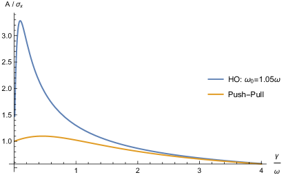
Figure S9: The signal-to-noise $A/\sigma_{x}$ as a function of $\gamma$ for the harmonic oscillator and the push-pull network. For the harmonic oscillator, the friction is varied, while $\omega_{0}$ is kept constant; for the push-pull network $\mu$ is varied according to $\mu=\omega_{0}^{2}/\gamma$. It is seen that for low and intermediate friction the harmonic oscillator outperforms the push-pull network, but that in the high-friction limit they perform similarly.

SII.4 Weakly non-linear oscillator and the coupled-hexamer model

The coupled-hexamer model (CHM) is a non-linear oscillator that can sustain autonomous limit-cycle oscillations in the absence of any driving. Here, we describe the Stuart-Landau model, which provides a universal description of a weakly non-linear system near the Hopf bifurcation where a limit cycle appears. We use it to analyze the time-keeping properties of a system as it is altered from essentially a damped linear oscillator to a weakly non-linear oscillator, see Fig. 3 of the main text. Our treatment follows largely that of Pikovsky et al. Pikovsky2003 .

SII.4.1 The amplitude equation

We consider the weakly non-linear oscillator Pikovsky2003 :

$$\ddot{x}+\omega_{0}^{2}x=f(x,\dot{x})+\rho s(t),$$ (S69)

with $s(t)=\sin(\omega t)+\bar{s}+\eta_{s}$ being the driving signal as before. The quantity $f(x,\dot{x})$ describes the non-linearity of the autonomous oscillator and the parameter $\rho$ controls the strength of the forcing. The description presented below is valid in the regime where the non-linearity $f(x,\dot{x})$ is small and the strength of the driving, quantified by $\rho$, is small. We begin by developing the formalism in the deterministic limit $\eta_{s}=0$, in which $s(t)$ is periodic with period $T=2\pi/\omega$, before returning to the effects of noisy driving. In contrast to previous sections, our discussion here is limited to input noise that is not only Gaussian but white, $\langle\eta_{s}(t)\rangle=0$ and $\langle\eta_{s}(t)\eta_{s}(t^{\prime})\rangle=\sigma_{s}^{2}\delta(t-t^{\prime})$.

Eq. S69 is close to that of a linear oscillator. We therefore expect that its solution has a nearly sinusoidal form. Moreover, we expect at least over some parameter range the frequency of the system is entrained by that of the driving signal. We therefore write the solution as

$$x(t)={\rm Re}\left[A(t)e^{i\omega t}\right]=\frac{1}{2}\left(A(t)e^{i\omega t}+{\rm c.c.}\right),$$ (S70)

where ${\rm c.c.}$ denotes complex conjugate. The above equation has the form of an harmonic oscillation with frequency $\omega$, but with a time-dependent complex amplitude $A(t)$. We emphasize that the observed frequency may deviate from $\omega$, when the amplitude $A(t)$ rotates in the complex plane.

The above equation determines only the real part of the complex number $A(t)e^{i\omega t}$. To fully specify $A(t)$, we also need to set the imaginary part of $A(t)e^{i\omega t}$, which we choose to do via

$$y(t) =-\omega{\rm Im}\left[A(t)e^{i\omega t}\right]=\frac{1}{2}\left(i\omega A(t)e^{i\omega t}+{\rm c.c.}\right)$$ (S71)

$$=\dot{x}.$$ (S72)

The relation $y(t)=\dot{x}$ thus specifies the imaginary part of the amplitude $A(t)$. Hence, the complex amplitude can be written as

$$A(t)e^{i\omega t}=x(t)-iy(t)/\omega.$$ (S73)

Writing $A(t)=R(t)e^{i\phi(t)}$, it can be verified that

$$x(t) =R(t)\cos(\phi(t)+\omega t)$$ (S74)

$$y(t) =-\omega R(t)\sin(\phi(t)+\omega t)$$ (S75)

$$R^{2}(t) =x^{2}(t)+y^{2}(t)/\omega^{2},$$ (S76)

and that the specification $\dot{x}(t)=y(t)$ implies that

$$\frac{\dot{R}(t)}{R(t)}=\dot{\phi}(t)\tan(\phi(t)+\omega t).$$ (S77)

Eq. S75 shows that the time derivative of $y(t)$ is

$$\dot{y} =-\omega^{2}x$$

$$-\omega\left[\dot{R}(t)\sin(\phi(t)+\omega t)+R(t)\dot{\phi}(t)\cos(\phi(t)+\omega t)\right]$$ (S78)

On the other hand, we know that

$$i\omega\dot{A}e^{i\omega t} =-\omega\left[\dot{R}(t)\sin(\phi(t)+\omega t)+R(t)\dot{\phi}(t)\cos(\phi(t)+\omega t)\right]$$

$$+i\omega\left[\dot{R}(t)\cos(\phi(t)+\omega t)-R(t)\dot{\phi}(t)\sin(\phi(t)+\omega t)\right]$$ (S79)

$$=\dot{y}+\omega^{2}x.$$ (S80)

where in Eq. S79 we have exploited that the imaginary part is zero because of Eq. S77. Combing the above equation with Eq. S69, noting that $\dot{y}=\ddot{x}$, yields the following equation for the time evolution of the amplitude:

$$\dot{A}=\frac{e^{-i\omega t}}{i\omega}\left[(\omega^{2}-\omega_{0}^{2})x+f(x,y)+\rho s(t)\right].$$ (S81)

SII.4.2 Averaging

The above transformation is exact. To make progress, we will use the method of averaging Guckenheimer:1983up . Specifically, we will time average Eq. S81 over one period $T$ Guckenheimer:1983up ; Pikovsky2003 . Averaging the driving $e^{-i\omega t}s(t)/(i\omega)$ yields the complex constant $E/(2\omega)$. The second term of Eq. S81 can be expanded in polynomials of $x(t)=(1/2){\rm Re}A(t)e^{i\omega t}$ and $y(t)=(1/2){\rm Im}A(t)e^{i\omega t}$, yielding powers of the type $(A(t)e^{i\omega t})^{n}(A^{*}(t)e^{-i\omega t})^{m}$. After multiplying with $e^{-i\omega t}$ and averaging over one period $T$, only the terms with $m=n-1$ do not vanish. Consequently, the terms that remain after averaging have the form $g(|A|^{2})A$, with an arbitrary function $g$. For small amplitudes only the linear term proportional to $A$ and the first non-linear term, $\propto|A|^{2}A$ term are important. Finally, averaging the first term of Eq. S81 yields a term linear in $A$.

Summing it up, the time evolution of the amplitude of the system with deterministic driving ($\eta_{s}=0$) is given by Pikovsky2003

$$\dot{A} =-i\frac{\omega^{2}-\omega_{0}^{2}}{2\omega}A+\alpha A-(\beta+i\kappa)|A|^{2}A-\frac{\rho}{2\omega}E$$ (S82)

The parameters have a clear interpretation. The parameters $\alpha$ and $\beta$ describe, respectively, the linear and non-linear growth or decay of oscillations. To have stable oscillations, both in the presence and absence of driving, large amplitude oscillations dominated by the nonlinear term need to decay, which means that $\beta$ must be positive, $\beta>0$; this parameter is fixed in all our calculations. The parameter that allows us to alter the system from one that shows damped oscillations in the absence of driving to one that can generate autonomous oscillations which do not rely on forcing, is $\alpha$. For the system to sustain free-running oscillations, small amplitude oscillations, dominated by the linear term, must grow, meaning that $\alpha$ must be positive, $\alpha>0$. The case with $\alpha>0$ thus describes a system that can perform stable limit cycle oscillations, making it a bonafide clock. The case $\alpha<0$ describes a system that in the absence of any driving, $E=0$, relaxes in an oscillatory fashion to a stable fixed point with $A=0$. In the presence of weak driving, the amplitude $A$ at the fixed point will be non-zero but small, making the effect of the non-linearity weak. The case $\alpha<0$ thus describes a system that is effectively a damped harmonic oscillator, which only dispays sustained oscillations when forced by an oscillatory signal. This system mimics the uncoupled-hexamer model.

The parameter $\kappa$ describes the non-linear dependence of the oscillation frequency on the amplitude. For the isochronous scenario in which the phase moves with a constant velocity, $\kappa=0$, which is what we will assume henceforth.

Defining the parameter $\nu\equiv(\omega^{2}-\omega_{0}^{2})/(2\omega)$ and the parameter $\epsilon\equiv\rho/(2\omega)$, we can then rewrite the above equation as

$$\dot{A}=-i\nu A+\alpha A-\beta|A|^{2}A-\epsilon E,$$ (S83)

where $A$ is the complex time-dependent amplitude, $E$ is a complex constant, and $\nu$, $\alpha$, and $\beta$ are real constants. Eq. S83 is Eq. 2 of the main text. It provides a universal description of a driven weakly nonlinear system near the Hopf bifurcation where the limit cycle appears Pikovsky2003 .

To model the input noise we will add the noise term to Eq. S83:

$$\dot{A}=-i\nu A+\alpha A-\beta|A|^{2}A-\epsilon E+\rho\bar{\eta}_{s}(t),$$ (S84)

where $\bar{\eta}_{s}(t)$ is the noise $\eta_{s}(t)$ averaged over one period of the driving:

$$\bar{\eta}_{s}(t)\equiv\frac{1}{T}\int_{t-T/2}^{t+T/2}dt^{\prime}\frac{e^{-i\omega t^{\prime}}}{i\omega}\eta_{s}(t^{\prime}).$$ (S85)

Since $\eta_{s}(t)$ is real but its prefactor $e^{-i\omega t}/{i\omega}$ is complex, $\bar{s}(t)$ is, in general, complex. Below we will describe the characteristics of the noise $\bar{\eta}_{s}$.

SII.4.3 Linear-Noise Approximation

Scenarios By varying $\alpha$ we will interpolate between two scenarios: the damped oscillator, modeling the UHM, with $\alpha<0$, and the weakly non-linear oscillator that can sustain free-running oscillations, modeling the CHM, with $\alpha>0$. For the system with $\alpha<0$, the amplitude of $x(t)$ when not driven is $A=0$: the system comes to a standstill. When the system is driven, the amplitude will be nonzero, but constant since the system is essentially linear as described above. For the system with $\alpha>0$, $A(t)$ can exhibit distinct types of dynamics, depending on the strength of driving and the frequency mismatch characterized by $\nu$ Pikovsky2003 . However, here we do not consider the regimes that $A(t)$ rotates in the complex plane; we will limit ourselves to the scenario that $A(t)=A$ is constant, meaning that $\nu$ cannot be too large Pikovsky2003 .

Overview Before we discuss the linear-noise approximation in detail, we first give an overview. The central observation is that both for the driven damped oscillator with $\alpha<0$ and the driven limit-cycle oscillator with $\alpha>0$, the complex amplitude $A$ is constant, corresponding to a stable fixed point of the amplitude equation, Eq. S83. In the spirit of the linear-noise approximation used to calculate noise in biochemical networks, we then expand around the fixed point to linear order, and evaluate the noise at the fixed point. This approach thus assumes that the distribution of the variables of interest is Gaussian, centered at the fixed point. More concretely, we first expand $A(t)$ to linear order around its stable fixed point, which is obtained by setting $\dot{A}$ in Eq. S83 to zero. This makes it possible to compute the variance of $A$. Importantly, this variance is that of a Gaussian distribution in the frame that co-rotates with the driving, as can be seen from Eqs. S74 and S75. To obtain the variance of $x$ and $y$ in the original frame, we then transform this distribution back to original frame of $x$ and $y$. If we can make this transformation linear, then it is guaranteed that the distribution of $x$ and $y$ will also be Gaussian. As we will see, the transformation can be made linear by writing $A$ as $A=u+iv$, where $u$ and $v$ are the real and imgainary parts of $A$, respectively.

Expanding $A$ around its fixed point We write $A(t)=u(t)+iv(t)$. Eq. S84 then yields for the real and imaginary part of $a(t)$:

$$\dot{u} =\nu v+\alpha u-\beta(u^{2}+v^{2})u-\epsilon e_{u}+\rho\bar{\eta}_{u}$$ (S86)

$$\dot{v} =-\nu u+\alpha v-\beta(u^{2}+v^{2})v-\epsilon e_{v}+\rho\bar{\eta}_{v}$$ (S87)

Here, $\bar{\eta}_{u}$ and $\bar{\eta}_{v}$ are the real and imaginary parts of the averaged noise $\bar{\eta}_{s}$, given by Eq. S85; they are discussed below. The quantities $e_{u}$ and $e_{v}$ are the real and imaginary parts of the driving $E$. Their respective values depend on the phase of the driving, which is arbitrary and can be chosen freely. For example, when the driving is $s(t)=\sin(\omega t)$, then $e_{u}=1$ and $e_{v}=0$, while if the signal is $s(t)=\cos(\omega t)$, then $e_{u}=0$ and $e_{v}=1$.

We now expand $u(t)$ and $v(t)$ around their steady-state values, $u^{\ast}$ and ${v^{\ast}}$, respectively. Inserting this in the above equations and expanding up to linear order yields

$$\dot{\delta u} =c_{1}\delta u+c_{2}\delta v+\rho\bar{\eta}_{u}$$ (S88)

$$\dot{\delta v} =c_{3}\delta u+c_{4}\delta v+\rho\bar{\eta}_{v},$$ (S89)

with

$$c_{1} =\alpha-\beta(3{u^{\ast}}^{2}+{v^{\ast}}^{2})$$ (S90)

$$c_{2} =\nu-\beta 2{u^{\ast}}{v^{\ast}}$$ (S91)

$$c_{3} =-\nu-\beta 2{u^{\ast}}{v^{\ast}}$$ (S92)

$$c_{4} =\alpha-\beta({u^{\ast}}^{2}+3{v^{\ast}}^{2}).$$ (S93)

The fixed points ${u^{\ast}}$ and ${v^{\ast}}$ are obtained by solving the cubic equations Eqs. S86 and S87 in steady state.

Noise characteristics We next have to specify the noise characteristics of $\bar{\eta}_{u}(t)$ and $\bar{\eta}_{v}(t)$. Eq. S85 reveals that the noise terms are given by

$$\bar{\eta}_{u}(t) =-\frac{1}{\omega T}\int_{t-T/2}^{t+T/2}dt^{\prime}\sin(\omega t^{\prime})\eta_{s}(t^{\prime})$$ (S94)

$$\bar{\eta}_{v}(t) =-\frac{1}{\omega T}\int_{t-T/2}^{t+T/2}dt^{\prime}\cos(\omega t^{\prime})\eta_{s}(t^{\prime}).$$ (S95)

The method of averaging Anishchenko:2007tf reveals that to leading order the statistics of these quantities can be approximated by

$$\langle\bar{\eta}_{u}(t)\bar{\eta}_{u}(t^{\prime})\rangle =\langle\bar{\eta}_{v}(t)\bar{\eta}_{v}(t^{\prime})\rangle=\frac{\sigma_{s}^{2}}{2\omega^{2}}\delta(t-t^{\prime})$$ (S96)

$$\langle\bar{\eta}_{u}(t)\bar{\eta}_{v}(t^{\prime})\rangle =0.$$ (S97)

Variance-co-variance From here, there are (at least) three ways to obtain the variance and co-variance matrix of $u$ and $v$. Since the system is linear, it can be directly solved in the time domain. Another route is via the power spectra TanaseNicola:2006bh ; Warren:2006ky . Here, we obtain it from Gardiner85

$${\bf A}{\bf C}_{uv}+{\bf C}_{uv}{\bf A^{\rm T}}=-{\bf D}_{uv}.$$ (S98)

The matrix ${\bf C}_{uv}$ is the variance-covariane matrix with elements $\sigma^{2}_{uu},\sigma^{2}_{uv},\sigma^{2}_{vu},\sigma^{2}_{vv}$ and ${\bf A}$ is the Jacobian of Eqs. S88 and S89 with elements $A_{11}=c_{1},A_{12}=c_{2},A_{21}=c_{3},A_{22}=c_{4}$. The matrix ${\bf D}_{uv}$ is the noise matrix of $\langle\bar{\eta}^{2}_{u/v}\rangle$, where we absorb the coupling strength $\rho=2\omega\epsilon$ (cf. Eq. S83) in the noise strength:

$${\bf D}_{uv} =\left(\begin{array}[]{cc}2\epsilon^{2}\sigma^{2}_{s}&0\\ 0&2\epsilon^{2}\sigma^{2}_{s}\end{array}\right).$$ (S101)

Transforming back The variance-covariance matrix ${\bf C}_{uv}$, with elements $\sigma^{2}_{uu},\sigma^{2}_{uv},\sigma^{2}_{vu},\sigma^{2}_{vv}$, characterizes a Gaussian distribution in the complex plane

$$P(u,v)=\frac{1}{2\pi\sqrt{|{\bf C}_{uv}|}}e^{-\frac{1}{2}{\bf a}^{\rm T}{\bf C}_{uv}^{-1}{\bf a}},$$ (S102)

where $|{\bf C}_{uv}|$ is the determinant of the variance-covariance matrix ${\bf C}_{uv}$ and ${\bf C}_{uv}^{-1}$ is the inverse of ${\bf C}_{uv}$, and ${\bf a}$ is a vector with elements $\delta u,\delta v$ (the deviations of the real and imaginary parts of $A=a$ from their respective fixed points ${u^{\ast}}$ and ${v^{\ast}}$) with ${\bf a}^{\rm T}$ its transpose. This distribution $P(u,v)$ defines a distribution in the co-rotating frame of the oscillator in the complex plane. To obtain $P(x,y)$ in the original non-co-rotating frame, we need to rotate this distribution. Eq. S73 shows that the corresponding rotation is described by

$$x(t) =u\cos(\omega t)-v\sin(\omega t)$$ (S103)

$$y(t) =-\omega u\sin(\omega t)-\omega v\cos(\omega t),$$ (S104)

which defines the rotation matrix

$${\bf Q}=\left(\begin{array}[]{cc}\cos(\omega t)&-\sin(\omega t)\\ -\omega\sin(\omega t)&-\omega\cos(\omega t)\end{array}\right)$$ (S107)

such that ${\bf z}={\bf Q}{\bf a}$, with ${\bf z}$ the vector with elements $\delta x(t)=x(t)-x^{\ast}(t),\delta y(t)=y(t)-y^{\ast}(t)$, where $x^{\ast},y^{\ast}$ are the rotating “fixed” points of $x(t)$ and $y(t)$, i.e. their time-dependent mean values, given by Eqs. S103 and S104 with $u=u^{\ast}$ and $v=v^{\ast}$. Hence, the distribution of interest is given by

$$P(x,y|t)=\frac{1}{2\pi\sqrt{|{\bf C}_{xy}|}}e^{-\frac{1}{2}{\bf z}^{\rm T}{\bf C}_{xy}^{-1}{\bf z}},$$ (S108)

where

$${\bf C}_{xy}^{-1}=[{\bf Q}^{-1}]^{\rm T}{\bf C}_{uv}^{-1}{\bf Q}^{-1}$$ (S109)

and its inverse ${\bf C}_{xy}$ is the variance-covariance matrix for $x,y$, with elements $\sigma^{2}_{xx}(t),\sigma^{2}_{xy}(t),\sigma^{2}_{yx}(t),\sigma^{2}_{yy}(t)$, which depend on time because ${\bf Q}$ depends on time.

Mutual information $I(p;t)$ Lastly, the oscillations in the phosphorylation $p(t)$ of the hexamer models correspond to the oscillations in $x(t)$ in the Stuart-Landau model. We therefore need to compute the mutual information $I(x;t)$, not $I(x,y;t)$. Specifically, we calculate the mutual information from

$$I(x,t)=H(x)-\langle H(x|t)\rangle_{t},$$ (S110)

where the entropy $H(x)=-\int dxP(x)\log P(x)$ with $P(x)=1/T\int_{0}^{T}dtP(x|t)$ and the conditional entropy $H(x|t)=-1/T\int_{0}^{T}dt\int dxP(x|t)\log P(x|t)$, with $P(x|t)=1/\sqrt{2\pi\sigma^{2}_{xx}(t)}e^{-(x(t)-x^{\ast}(t))^{2}/(2\sigma^{2}_{xx}(t))}$. We emphasize that both the variance $\sigma^{2}_{xx}(t)$ and the average $x^{\ast}(t)$ depend on time.

Summing up Approach and Parameters Fig. 3 main text To sum up the procedure, to compute the noise in $A=a$ we first need to obtain the steady state values of its real and imaginary part, $\bar{u}$ and $\bar{v}$ (see Eqs. S90-S93). These are obtained from setting the time derivatives of $u(t)$ and $v(t)$ in Eqs. S86 and S87 to zero; this involves solving a cubic equation, which we do numerically. We then compute the variance-covariance matrix ${\bf C}_{uv}$ via Eq. S98, where the elements of the Jacobian ${\bf A}$ are given by Eqs. S90-S93 and the noise matrix ${\bf D}_{uv}$ is given by Eq. S101. After having obtained ${\bf C}_{uv}$, we find the variance-covariance matrix for $x$ and $y$, ${\bf C}_{xy}$, from Eq. S109. For Fig. 3 of the main text, $\nu=0$, $\beta=\omega$, $\epsilon=0.5\omega$.

SII.4.4 Comparing limit cycle oscillator with damped oscillator

Fig. 3 of the main text shows that the mutual information $I(x;t)$ increases with $\alpha$, especially when the input noise is large. To elucidate this further, we show in Fig. S10 for two different values of $\alpha$ and for two levels of the input noise, the dynamics of the system in the plane of $x$ and $y$. The panels not only show the mean trajectory, indicated by the dashed line, but also samples $(x,y)$ from $P(x,y|t_{i})$ for evenly spaced time points $t_{i}$; $P(x,y|t)$ is given by Eq. S108 and samples from the same time point $t_{i}$ have the same color. It is seen that when the input noise is low (left two panels), the respective distributions (“blobs”) are well separated, both for $\alpha=-\omega$, when the system is a damped oscillator (D.O.) (top row), and for $\alpha=3\omega$ (bottom row), when the system is a limit-cycle oscillator (L.C.O.). However, when the input noise is large (right column), the blobs of the damped oscillator become mixed, while the distributions $P(x,y|t)$ of the limit-cycle oscillator are still fairly well separated.

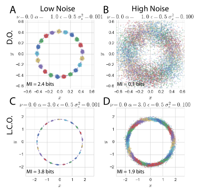
Figure S10: The dynamics of the Stuart-Landau model when $\alpha=-\omega$, corresponding to a damped oscillator (D.O., top row), and when $\alpha=3\omega$, corresponding to a limit-cycle oscillator (L.C.O.,bottom row), both for low input noise, $\sigma^{2}_{s}=0.001\omega$ (left column) and high input noise, $\sigma^{2}_{s}=0.1\omega$ (right column). Dashed line denotes the mean trajectory of $(x,y)$, and the points are samples of $(x,y)$ from the distribution $P(x,y|t_{i})$ for evenly spaced time points $t_{i}$; $P(x,y|t)$ is given by Eq. S108 and points belonging to the same time have the same color. It is seen that when the input noise is low, the distributions corresponding to the different times are still well separated, both for the limit-cycle oscillator and the damped oscillator. Yet, for high noise, only for the L.C.O. are the distributions still reasonably separated, leading to a mutual information that is still close to 2 bits. In contrast, for the D.O., the distributions are mixed, leading to a low mutual information close to zero.

To interpret this further, we note that the mutual information $I(x;t)=H(t)-H(t|x)$. Here, $H(t)$ is the entropy of the input signal, which is constant, i.e. does not depend on the design of the system. The dependence of $I(x;t)$ on the design of the system is thus governed by the conditional entropy, given by $H(t|x)=\langle\langle-\log P(t|x)\rangle_{P(t|x)}\rangle_{P(x)}$. The quantity $\langle-\log P(t|x)\rangle_{P(t|x)}$ quantifies the uncertainty in estimating the time $t$ from a given output $x$; the average $\langle\dots\rangle_{P(x)}$ indicates that this uncertainty should be averaged over all output values $x$ weighted by $P(x)$. The conditional entropy $H(t|x)$ is low and $I(x;t)$ is high when, averaged over $x$, the distribution $P(t|x)$ of times $t$ for a given $x$ is narrow. We can now interpret Fig. S10: The smaller the number of blobs that intersect the line $x$, the higher the mutual information. Or, concomitantly, the more the distributions are separated, the higher the mutual information—information transmission is indeed a packing problem. Clearly, when the input noise is low, the time can be inferred reliably from the output even with a damped oscillator (top left panel). For high input noise, however, the mutual information of the damped oscillator falls dramatically because the blobs now overlap strongly. In contrast, the distributions of the limit-cycle oscillator are still reasonably separated and $I(x;t)$ is still almost close to 2 bits.

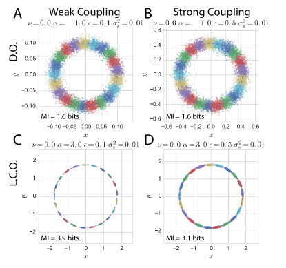
Figure S11: The dynamics of the Stuart-Landau model when $\alpha=-\omega$, corresponding to a damped oscillator (D.O., top row), and when $\alpha=3\omega$, corresponding to a limit-cycle oscillator (L.C.O., bottom row), both for weak coupling, $\epsilon=0.1\omega$ (left column) and strong coupling, $\epsilon=0.5\omega$ (right column); the input noise is set to a low value, $\sigma^{2}_{s}=0.01\omega$. Dashed line denotes the mean trajectory of $(x,y)$, and the points are samples of $(x,y)$ from the distribution $P(x,y|t_{i})$ for evenly spaced times $t_{i}$; $P(x,y|t)$ is given by Eq. S108 and points belonging to the same time have the same color. It is seen that for the D.O. the amplitude and the noise are small when the coupling is small (top left panel; note the scale on the x- and y-axis). Increasing the coupling, however, not only raises the amplitude (the gain), but also amplifies the noise, leaving the mutual information unchanged: a damped oscillator cannot lift the trade-off between gain and noise. In contrast, the limit-cycle oscillator already exhibits large amplitude oscillations even for weak coupling; at the same time, lowering the coupling strength does reduce input-noise propagation. The limit-cycle oscillator can thus lift the trade-off between gain and input: lowering the coupling raises the mutual information. Section SII.5 makes these arguments quantitative. It is also interesting to note that especially the fluctuations in the radial direction, the amplitude fluctuations, are strongly reduced in the L.C.O., due to the non-linearity of the system.

Fig. S10 also nicely illustrates that the mutual information would be increased if the system could estimate the time not from $x$ only, but instead from $x$ and $y$: this removes the degeneracy in estimating $t$ for a given $x$ associated with sinusoidal oscillations Monti:2016bp . One mechanism to remove the degeneracy is to have a readout system that not only reads out the amplitude of the clock signal, but also its derivative, for example via incoherent feedback loops Becker:2015iu . Another possibility is that the clock signal is read out by 2 (or more) proteins that are out of phase with each other, as shown in Monti:2016bp . Indeed, while we have computed the instantaneous mutual information between time and the output at a given time, the trajectory of the clock signal provides more information about time, which could in principle be extracted by appropriate readout systens Monti:2016bp .

Lastly, we show in Fig. S11 the dynamics for two different values of $\alpha$ and for two different values of the coupling strength $\epsilon$. The top left panel shows that when $\epsilon$ is small, the amplitude of the damped oscillator is very weak—note the scale on the x- and y-axis. To increase the amplitude of the output, the coupling strength must be increased. However, this amplifies the input noise as well, such that the mutual information remains unchanged (top right panel): the damped oscillator faces a fundamental trade-off between gain and input noise that cannot be lifted. In contrast, the limit-cycle oscillator (bottom row) already exhibits strong amplitude oscillations even when the coupling strength $\epsilon$ is small: the amplitude of the cycle—a bonafide limit-cycle—is determined by the properties of the system, and is only very weakly affected by the strength of the forcing. At the same time, weakening the coupling does reduce the propagation of input noise. These two observations together explain why for the limit-cycle oscillator the mutual information increases as the coupling is reduced. In SII.5 we elucidate these arguments further, and show that concerning the robustness to input noise, the weak-coupling regime is the optimal regime that maximizes the mutual information, and that in this regime a limit-cycle oscillator is superior over a damped oscillator.

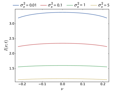
Figure S12: The mutual information $I(x;t)$ in the Stuart-Landau model as a function of $\nu=(\omega^{2}-\omega_{0}^{2})/(2\omega)$, for different input-noise strengths $\sigma^{2}_{s}$. It is seen that the mutual information is maximized at $\nu=0$ (corresponding to $\omega_{0}=\omega$) for all input noise levels. $\beta=1.0\omega$; $\epsilon=0.5\omega$; $\alpha=3\omega$; $\sigma^{2}_{s}$ in units of $\omega$.

SII.4.5 Optimal intrinsic frequency

Fig. S3B shows that the optimal intrinsic frequency $\omega_{0}^{\rm opt}$ that maximizes the mutual information $I(p;t)$ for the coupled-hexamer model (CHM) depends, albeit very weakly, on the input-noise strength $\sigma^{2}_{s}$. Here we wondered whether the Stuart-Landau model could reproduce this feature. Fig. S12 shows the result. The figure shows the mutual information $I(x;t)$ as a function of $\nu=(\omega^{2}-\omega_{0}^{2})/(2\omega)$ for different values of $\sigma^{2}_{s}$. It is seen that the dependence of $I(x;t)$ on $\nu$ is rather weak, yielding a broad maximum that peaks at $\nu=0$ (corresponding to $\omega_{0}=\omega$) for all noise strengths. This suggests that the optimal $\omega_{0}^{\rm opt}<\omega$ observed for low input noise in the CHM arises from a stronger non-linearity in that system than captured by the Stuart-Landau model, which describes weakly non-linear oscillators.

SII.5 Why limit cycle oscillators are generically more robust to input noise than damped oscillators in the weak-coupling regime

The principal result of our manuscript, illustrated in Fig. 2 of the main text, is that a limit-cycle oscillator is more robust to input noise than a damped oscillator. We now address the question how generic this observation is, and whether it can explained from a simple scaling argument. To answer these questions, we will investigate the analytical models discussed in the previous sections, which are valid in the regime of weak coupling. We will analyse the harmonic oscillator described in SII.2, which applies not only to the uncoupled hexamer model (UHM), but also, in the high-friction limit, to the push-pull network (PPN), as described in SII.3. For the coupled-hexamer model, we will analyse not only the Stuart-Landau model described in SII.4, but also a phase-oscillator model within the phase-averaging approximation Monti:2018hs . While the Stuart-Landau model gives a universal description of weakly non-linear oscillators near the Hopf bifurcation, the phase-oscillator model within the phase-averaging approximation gives a general description of (potentially highly) non-linear oscillators in the weak coupling regime Monti:2018hs ; importantly, both descriptions give the same scaling argument, strongly suggesting it applies to most, if not all, limit-cycle oscillators. The principal finding of our analysis of these models is that damped oscillators such as the UHM and PPN cannot lift the trade-off between the amplification of the output signal (the gain) and the propagation of input noise, while limit-cycle oscillators can because their oscillations have an inherent robust amplitude, which does not rely on external driving. Before we derive the principal result in detail in the paragraphs below, we first give an overview of the main arguments, for the case where there is no internal noise. In the next section (SII.6), we then discuss the role of internal noise and how the optimal design of the readout system depends on the relative amounts of internal and external noise.

Overview To understand why limit-cycle oscillators (CHM) are generically more robust to input noise than damped oscillators (UHM and PPN), the role of the coupling strength $\rho$ is key. For a damped oscillator, the amplitude $A$ of the output oscillations (the signal) scales linearly with the coupling strength, $A\sim\rho$. However, increasing the coupling not only amplifies the signal, but also the input noise. Moreover, it does so by the same amount: the standard deviation of the output signal, $\sigma_{x}$ also scales linearly with $\rho$, $\sigma_{x}\sim\rho$. Consequently, the number of distinct time points that can be resolved, the signal-to-noise ratio $A/\sigma_{x}$, is independent of $\rho$: damped oscillators cannot lift the trade-off between gain and input noise by optimizing the coupling strength, as can also be seen in panels A and B of Fig. S11.

This is in marked contrast to the behavior of a limit-cycle oscillator. A limit-cycle oscillator has an intrinsic amplitude $A$, which does not rely on external driving, as the amplitude of a damped oscillator does. Its amplitude is thus essentially independent of $\rho$, and, more specifically, it goes to a non-zero value as $\rho\to 0$. Moreover, while the amplitude remains finite, the propagation of input noise does go to zero as $\rho\to 0$, because, as we will show, $\sigma_{x}\sim\sqrt{\rho}$. Hence, the signal-to-noise ratio $A/\sigma_{x}\sim 1/\sqrt{\rho}$ rises as the coupling is decreased, as Fig. S11C/D illustrate. Although this scaling law naively suggests that the optimal coupling strength is $\rho\rightarrow 0$, we will show below that, in real systems, internal noise and detuning between the driving and intrinsic oscillator frequencies always cut off the divergence at small but finite $\rho$.

Importantly, we find exactly the same scaling relation $A/\sigma_{x}\sim 1/\sqrt{\rho}$ for both the Stuart-Landau model and the phase-oscillator model within the phase-averaging approximation, which is the natural description of non-linear limit-cycle oscillators in the weak-coupling regime Pikovsky2003 ; Monti:2018hs . Our analysis thus shows that concerning the robustness to input noise: 1) the optimal regime that maximizes the signal-to-noise ratio is the weak-coupling regime; 2) in this regime, limit-cycle oscillators are generically more robust than damped oscillators. We emphasize that the weak-coupling regime is precisely the regime where our analysis applies, indicating that our principal result applies to a very broad class of oscillators. Moreover, this result can be understood intuitively: while both a damped and a limit-cycle oscillator can reduce the propagation of input noise by lowering the coupling strength, only the limit-cycle oscillator still exhibits a robust amplitude in the weak-coupling regime, raising the signal-to-noise ratio (see Fig. S11). In the next paragraphs, we derive and elucidate the scaling of $A$ and $\sigma_{x}$ with $\rho$ for both oscillator models. The role of internal noise is discussed in the next section.

Damped oscillators We will first reiterate the main findings for the harmonic oscillator (the uncoupled hexamer model), described in SII.2; these findings also apply to the push-pull network, which corresponds to the high-friction limit of the harmonic oscillator (see section SII.3). The amplitude of the harmonic oscillator is given by Eq. S56 and repeated here for completeness:

$$A =\frac{\rho}{\sqrt{\gamma^{2}\omega^{2}+(\omega^{2}-\omega_{0}^{2})^{2}}}\sim\rho.$$ (S111)

Importantly, the amplitude increases linearly with the coupling strength $\rho$. This result can be understood by noting that the driving force $\rho s(t)$ scales with $\rho$ while the restoring force $-\omega_{0}^{2}x$ is independent of $\rho$ (see Eq. S46). The variance $\sigma^{2}_{x}$ of the output is, for Gaussian white input noise of strength $\sigma^{2}_{s}$ (see Eq. S62):

$$\sigma^{2}_{x} =\frac{\rho^{2}\sigma^{2}_{s}}{2\gamma\omega_{0}^{2}}\sim\rho^{2}.$$ (S112)

Clearly, the noise in the output $\sigma_{x}$ scales with the coupling strength $\rho$. This is because increasing the coupling strength not only amplifies the true signal $\sin(\omega t)$ but also the noise in the input signal, $\eta_{s}$ (see Eq. S46). Because both the amplitude $A$ and the noise $\sigma_{x}$ scale with the couplgin strength $\rho$, the signal-to-noise ratio is independent of the coupling strength $\rho$:

$$\frac{A}{\sigma_{x}} =\frac{\sqrt{2\gamma}\omega_{0}}{\sigma_{s}\sqrt{\gamma^{2}\omega^{2}+(\omega^{2}-\omega_{0}^{2})^{2}}}\sim\rho^{0}.$$ (S113)

Indeed, these systems cannot lift the trade-off between gain and noise: amplifying the signal inevitably also amplifies the noise in the input. This is in marked contrast to the limit-cycle oscillators, as we show next.

Limit-cycle oscillator: Stuart-Landau model To develop our argument, we consider the case that the frequency mismatch $\nu=(\omega^{2}-\omega_{0}^{2})/(2\omega)=0$. Moreover, we choose the phase of the driving signal such that $e_{v}=0$, as a result of which $v^{\ast}=0$ (see Eq. S87). With $v^{\ast}=0$, the steady-state value of the phase is $\phi^{\ast}=0$, while the mean amplitude of the limit cycle becomes $R^{\ast}=|u^{\ast}|$. Importantly, this amplitude, which can be obtained by solving the cubic equation for $u$ (Eq. S86) is very insensitive to the coupling strength $\rho$—this is indeed a hallmark of a limit-cycle oscillator. As a result, even for the weakest coupling strengths $\rho$, the system exhibits a robust amplitude $A=R^{\ast}$, as illustrated in Fig. S11C/D. Since with $v^{\ast}=0$ the amplitude is $R^{\ast}=|u^{\ast}|$, its variance is $\sigma^{2}_{R}=\sigma^{2}_{u}$. Moreover, the variance in the phase is $\sigma^{2}_{\phi}=\sigma^{2}_{v}/{R^{\ast}}^{2}$. With $\nu=0$ and $v^{\ast}=0$, $c_{2}$ and $c_{3}$ in Eqs. S90-S93 are both zero, which then yields the following expressions for the variance in $u$ and $v$ (using that $\epsilon\equiv\rho/(2\omega)$):

$$\sigma^{2}_{u} =\frac{\rho^{2}\sigma^{2}_{s}}{4(-\alpha+\beta 3{u^{\ast}}^{2})\omega^{2}}$$ (S114)

$$\sigma^{2}_{v} =\frac{\rho^{2}\sigma^{2}_{s}}{4(-\alpha+\beta{u^{\ast}}^{2})\omega^{2}}.$$ (S115)

Before we discuss the signal-to-noise ratio in the limit-cycle oscillator, we note that for a harmonic oscillator with $\beta=0$, the method of averaging yields $\alpha=-\gamma/2$, showing that the result above indeed reduces to that for a harmonic oscillator with $\omega_{0}=\omega$ (see Eq. S112). We now analyze the numerator and denominator of Eqs. S114 and S115 for the limit-cycle oscillator with $\beta>0$. The numerator increases with the coupling strength $\rho$, as observed for the harmonic oscillator; this reflects the fact that also in the limit-cycle oscillator, the input fluctuations are amplified by the gain $\rho$. This numerator is the same for both $\sigma^{2}_{u}$ and $\sigma^{2}_{v}$. The denominator, however, is larger for $\sigma^{2}_{u}$ than for $\sigma^{2}_{v}$. Indeed, the restoring force for amplitude fluctuations, corresponding to $\sigma^{2}_{u}=\sigma^{2}_{R}$, is larger than that for the phase fluctuations, $\sigma^{2}_{\phi}=\sigma^{2}_{v}/{R^{\ast}}^{2}$. This is the remnant of the fact that limit-cycle oscillators, in the absence of any driving, exhibit a neutral mode in the direction along the limit cycle; even with the coupling, this thus remains the soft mode. It is predominantly these fluctuations, $\sigma^{2}_{v}$, that limit the precision in estimating the time. Interestingly, since we have chosen the phase of the input such that $v^{\ast}=0$ and $R^{\ast}=|u^{\ast}|$, an inspection of Eq. S86 shows that $-\alpha+\beta{u^{\ast}}^{2}=\epsilon/R^{\ast}=\rho/(2\omega R^{\ast})$. Hence, we find that

$$\sigma^{2}_{v}=\frac{\rho^{2}\sigma^{2}_{s}R^{\ast}}{2\rho\omega}\sim\rho.$$ (S116)

The expression shows that the coupling not only amplifies the input noise (the numerator), but also that it generates a restoring force that tames these fluctuations (the denominator). The latter is in marked contrast to the harmonic oscillator, which lacks this restoring force (see Eq. S112). Consequently, while the output noise $\sigma^{2}_{x}$ of the harmonic oscillator scales as $\rho^{2}$ (Eq. S112), that of the limit-cycle oscillator scales as $\rho$. We also note that the restoring force decreases with the amplitude $R^{\ast}$ of the limit cycle.

Eq. S116 shows that the signal-to-noise ratio $A/\sigma_{v}=R^{\ast}/\sigma_{v}$ is given by

$$\frac{A}{\sigma_{v}}=\frac{1}{\sigma_{s}}\sqrt{\frac{2\omega R^{\ast}}{\rho}}\sim\frac{1}{\sqrt{\rho}},$$ (S117)

where we have used that for small $\rho$ the amplitude $R^{\ast}$ has a finite value. Clearly, in the weak coupling limit, the signal-to-noise ratio of the limit-cycle oscillator increases as $\rho$ decreases, in contrast to the signal-to-noise ratio of the damped oscillator, which is independent of $\rho$ (Eq. S113). As a result, for sufficiently weak coupling, a limit-cycle oscillator will inevitably become superior to a damped oscillator. Fundamentally, the reason is that the limit-cycle oscillator has an intrinsic amplitude which does not rely on external driving, while the damped oscillator does not: in both systems the input fluctuations are only weakly amplified in the weak-coupling regime, but only the limit-cycle oscillator has in this regime still a strong amplitude that raises the signal above the noise.

We can also obtain a signal-to-noise ratio by dividing the amplitude of the limit-cycle $A=2\pi$ by the standard deviation of the phase, $\sigma_{\phi}=\sigma_{v}/R^{\ast}$:

$$\frac{A}{\sigma_{\phi}}=\frac{2\pi}{\sigma_{s}}\sqrt{\frac{2\omega R^{\ast}}{\rho}}$$ (S118)

This indeed gives the same scaling with the coupling constant $\rho$ and the radius of the limit cycle $R^{\ast}$.

Limit-cycle oscillator: Phase-averaging method The Stuart-Landau model describes a weakly non-linear system near the Hopf bifurcation. Yet, the coupled-hexamer model exhibits large-amplitude oscillations. We therefore also investigate a phase-oscillator model, which describes non-linear oscillators with a robust limit cycle. We analyze this model via the phase-averaging method, which applies in the regime that the intrinsic frequency $\omega_{0}$ is close to the driving frequency $\omega$ and the coupling $\rho$ is weak Pikovsky2003 ; Monti:2018hs . This framework provides a description of the dynamics of the phase difference $\psi\equiv\phi-\omega t$ between the phase of the clock, $\phi$, and that of the external signal $\omega t$:

$$\dot{\psi}=\nu+\rho_{\psi}Q(\psi)+\rho_{\psi}\eta_{s},$$ (S119)

where, as before, $\nu=(\omega^{2}-\omega^{2}_{0})/(2\omega)$, $\eta_{\psi}$ is a Gaussian white noise source $\langle\eta_{\psi}(t)\eta_{\psi}(t^{\prime})\rangle=\sigma^{2}_{s}\delta(t-t^{\prime})$, $\rho_{\psi}$ is the coupling strength, and $Q(\psi)=\int_{0}^{T}dt^{\prime}Z(\psi+\omega t^{\prime})s(t^{\prime})$ is the force acting on $\psi$, given by the convolution of instantaneous phase-response curve $Z(\phi)$ and the driving signal $s(t)$ Pikovsky2003 ; Monti:2018hs . In the phase-locked regime, the deterministic equation $\dot{\psi}=\nu+\rho_{\psi}Q(\psi)$ always has a stable fixed point $\psi^{*}$. Linearizing about this fixed point, we find:

$$\dot{\delta\psi}=-\rho_{\psi}\zeta\delta\psi+\rho\eta_{\psi},$$ (S120)

where $\zeta$ is the linearization of the force $Q(\psi)$ around the fixed point $\psi^{*}$. From this we obtain for the variance

$$\sigma^{2}_{\psi}=\frac{\rho_{\psi}^{2}\sigma^{2}_{s}}{2\rho_{\psi}\zeta}\sim\rho_{\psi}.$$ (S121)

We note that, as in the Stuart-Landau description (see Eq. S116), the numerator scales with $\rho_{\psi}^{2}$, because of the amplification of the input fluctuations. The denominator scales, as in the Stuart-Landau model, with $\rho_{\psi}$, reflecting the fact that the restoring force that tames fluctuations in $\psi$ increases with the coupling strength $\rho_{\psi}$. In fact, not only the scaling with $\rho$ is the same in the Stuart-Landau model and the phase-averaging method, but also the scaling with $R^{\ast}$; this can be understood by noting that $\rho_{\psi}=\rho/R^{\ast}$, which comes from the factor $\partial\phi/\partial x$ that arises in reducing the dynamics of $x$ to that of $\phi$ and $\psi$ see Pikovsky2003 ; Monti:2018hs .

The amplitude of the limit cycle $A=2\pi$ is constant. This means that in this description, the signal-to-noise ratio—the number of time points that can be inferred from the phase $\psi$—scales as

$$\frac{A}{\sigma_{\psi}}\sim\frac{1}{\sqrt{\rho}}.$$ (S122)

Hence, as found for the Stuart-Landau model (Eq. S117), also in this description the signal-to-noise ratio of a limit-cycle oscillator increases as the coupling strength decreases, in contrast to that of a damped oscillator for which the signal-to-noise ratio is independent of coupling strength.

Role of detuning Lastly, while a finite detuning $\nu\neq 0$ necessitates a minimal coupling strength $\rho$ to bring the system inside the Arnold tongue, as illustrated in Fig. S3D, Eq. S120 indicates that inside the Arnold tongue the scaling of the signal-to-noise ratio $A/\sigma_{\psi}$ with $\rho$ does not depend on the amount of detuning $\nu$—the detuning generates a constant force which affects the fixed point $\psi^{\ast}$, but it does not affect the restoring force for fluctuations around $\psi^{\ast}$.

SII.6 Role of internal noise

In the above sections we studied the robustness of the three different systems to input noise. We now address the role of internal noise, which arises from the intrinsic stochasticity of chemical reactions. First, in the next section, we study the signal-to-noise ratio of these systems in the presence of internal noise only. In the subsequent section, we then address their performance in the presence of both internal and input noise. The coupled-hexamer model is again described by the Stuart-Landau model and the phase-averaging method of the previous section, while the push-pull network and the uncoupled-hexamer model are described by the damped oscillator of section SII.2; the latter system describes not only the uncoupled-hexamer model, but also, in the high-friction limit, the push-pull network of SII.1 (see also SII.3).

SII.6.1 Robustness to internal noise

The derivation of the signal-to-noise ratio of the respective systems in the presence of internal noise closely follows that on input noise: the principal difference concerns the scaling of the noise with the coupling strength.

Damped oscillator To study the role of internal noise, we can add an intrinsic noise term to Eq. S46. This will yield the same expression for $\dot{x}$ as that in the presence of external noise, except that the external noise term scales with the coupling strength $\rho$, while the internal noise term does not. Hence, we find for the variance of the output $\sigma^{2}_{x}$ in the presence of internal Gaussian white noise of strength $\sigma^{2}_{\rm int}$:

$$\sigma^{2}_{x} =\frac{\sigma^{2}_{\rm int}}{2\gamma\omega_{0}^{2}}.$$ (S123)

Note that the noise $\sigma^{2}_{x}$ is independent of the coupling strength.

The expression for the amplitude is still given by Eq. S56 (Eq. S111). Combining this expression with Eq. S123 then yields the following expression for the signal-to-noise ratio for the damped oscillator with internal noise only:

$$\frac{A}{\sigma_{x}} =\frac{\sqrt{2\gamma}\omega_{0}\rho}{\sigma_{\rm int}\sqrt{\gamma^{2}\omega^{2}+(\omega^{2}-\omega_{0}^{2})^{2}}}\sim\rho.$$ (S124)

Clearly, the signal-to-noise ratio now increases with the coupling strength $\rho$. Whereas with input noise both the noise $\sigma_{x}$ and the amplitude $A$ scale with $\rho$ such that the signal-to-noise ratio is independent of $\rho$, with internal noise the amplitude $A$ scales with $\rho$ but the noise $\sigma_{x}$ does not; increasing the coupling thus makes it possible to raise the output signal above the internal noise.

Limit-cycle oscillator: Stuart-Landau model Also for the Stuart-Landau model, the principal difference between the internal and input noise is that the former does not scale with the coupling strength $\rho$ while the latter does. Following the steps from Eq. S114 to Eq. S116, but with the effective input noise $\rho^{2}\sigma^{2}_{s}$ replaced by the internal noise $\sigma^{2}_{\rm int}$, we find that in the presence of internal noise, the output noise is given by

$$\sigma^{2}_{v}=\frac{\sigma^{2}_{\rm int}R^{\ast}}{2\rho\omega}.$$ (S125)

Importantly, $\sigma^{2}_{v}$ decreases as the coupling $\rho$ is increased. As we have seen above for the case of input noise, Eq. S116, for the limit-cycle oscillator the coupling to the input yields a restoring force that increases with $\rho$.

With the amplitude $A=R^{\ast}$, we then obtain the following signal-to-noise ratio:

$$\frac{A}{\sigma_{v}}=\frac{\sqrt{2\rho\omega R^{\ast}}}{\sigma_{\rm int}}\sim\sqrt{\rho}.$$ (S126)

Before we discuss the scaling of the signal-to-noise ratio with $\rho$, we first note that by replacing $\rho_{\psi}^{2}\sigma^{2}_{s}$ by $\sigma^{2}_{\rm int}$ in Eq. S121, we see that the phase-averaging method yields the same scaling of the output noise and hence the signal-to-noise ratio with $\rho$ as the Stuart-Landau model does.

Eq. S126 shows that increasing the coupling of the limit-cycle oscillator to the input raises the signal-to-noise ratio, as it does for the damped oscillator (Eq. S124). However, the origin is markedly different: for the damped oscillator, a stronger coupling yields a larger amplitude (Eq. S111) while the noise $\sigma_{x}$ (Eq. S123) remains constant, whereas for the limit-cycle oscillator the amplitude is essentially unaffected by the coupling yet the noise (Eq. S125) decreases as $\rho$ increases, because of the larger restoring force. This difference manifests itself in a different scaling with $\rho$, which has an interesting consequence: Because the signal-to-noise ratio of the limit-cycle oscillator scales with $\sqrt{\rho}$ while that of the damped oscillator scales with $\rho$, in the weak-coupling regime the limit-cycle oscillator will not only be more robust to input noise, as discussed in the previous section, but will also be more resilient to internal noise.

However, this analysis also shows that the regime of weak coupling is not necessarily the optimal one: increasing $\rho$ enhances the suppression of internal noise. It should be realized, however, that the analysis presented here is an analysis that strictly applies only in the regime of weak coupling. Indeed, for large coupling other effects which are not captured by our analysis will inevitably come into play. For example, the output signal becomes non-sinusoidal because of the fact that the phosphorylation level $p(t)$ is bounded between zero and unity; these non-sinusoidal oscillations tend to reduce information transmission Monti:2018hs . Moreover, combining the observations from the previous section on input-noise propagation, which decreases as the coupling $\rho$ is decreased, and the observations above on the suppression of internal noise, which increases with $\rho$, predicts that in the presence of both noise sources there exists an optimal coupling strength that maximizes the mutual information. In addition, it predicts that the magnitude of the optimal coupling strength depends on the relative amounts of input noise and internal noise. This is what we show in the next section.

SII.6.2 Signal-to-noise ratio in presence of input noise and internal noise

Damped oscillator In the presence of both internal and external noise, the noise of the output of the damped oscillator is, combining Eqs. S112 and S123:

$$\sigma^{2}_{x}=\frac{\rho^{2}\sigma^{2}_{s}}{2\gamma\omega_{0}^{2}}+\frac{\sigma^{2}_{\rm int}}{2\gamma\omega_{0}^{2}}.$$ (S127)

Note that for small coupling strength $\rho$ the internal noise (second term) dominates, while for large $\rho$ the input noise dominates.

Combining this expression with that for the amplitude, Eq. S56, yields the following signal-to-noise ratio

$$\frac{A}{\sigma_{x}} =\frac{\sqrt{2\gamma}\omega_{0}\rho}{\sqrt{\rho^{2}\sigma^{2}_{s}+\sigma^{2}_{\rm int}}\sqrt{\gamma^{2}\omega^{2}+(\omega^{2}-\omega_{0}^{2})^{2}}}\sim\frac{a\rho}{\sqrt{b\rho^{2}+c}},$$ (S128)

where $a$, $b$, and $c$ are constants independent of $\rho$. Hence, for small $\rho$, the signal-to-noise ratio scales linearly with $\rho$ because in this regime the rise of the amplitude $A$ with $\rho$ makes it possible to lift the signal above the internal noise. Yet, for large $\rho$, the signal-to-noise ratio becomes independent of $\rho$, because then the external noise dominates, which scales with $\rho$ in the same way as the amplitude does. We emphasize that these calculations pertain to the push-pull network (PPN) and the uncoupled-hexamer model (UHM) provided that these systems remain in the linear-response regime; as discussed in the previous section (see also section SI.5), for very large coupling, the push-pull network and uncoupled-hexamer model will be driven out of the linear-response regime because the output $p(t)$ is bounded from above and below; this reduces information transmission. We thus expect a broad plateau, precisely as the simulation data of the PPN and UHM show (Fig. S4A/B).

Limit-cycle oscillator: Stuart-Landau model In the presence of both input and internal noise, the output noise in the Stuart-Landau model is, combining Eqs. S116 and S125:

$$\sigma^{2}_{v}=\frac{\rho\sigma^{2}_{s}R^{\ast}}{2\omega}+\frac{\sigma^{2}_{\rm int}R^{\ast}}{2\rho\omega}.$$ (S129)

While the first term (the input noise) scales with $\rho$ because the coupling amplifies the input noise more than the restoring force tames it (see discussion below Eq. S116), the second term decreases with $\rho$ because of the restoring force. This expression yields for the signal-to-noise ratio $A/\sigma_{v}=R^{\ast}/\sigma_{v}$

$$\frac{A}{\sigma_{v}}=\sqrt{\frac{2\rho\omega R^{\ast}}{\rho^{2}\sigma^{2}_{s}+\sigma^{2}_{\rm int}}}\sim\sqrt{\frac{a\rho}{b\rho^{2}+c}}.$$ (S130)

It is seen that the signal-to-noise ratio increases with the coupling strength for small $\rho$, scaling as $\sqrt{\rho}$, because for weak coupling the intrinsic noise dominates over the input noise, and increasing the coupling raises the restoring force that contains these fluctuations. In the large coupling regime, the input noise will dominate and then the signal-to-noise ratio will decrease with $\rho$ as $1/\sqrt{\rho}$—while the amplitude is essentially independent of $\rho$, increasig $\rho$ amplifies the propagation of the input fluctuations. This equation thus predicts a pronounced maximum in the signal-to-noise ratio for the limit-cycle oscillator, as, in fact, observed for the coupled-hexamer model, see Fig. S4C. Since the phase-averaging method yields the same scaling with $\rho$ for both the internal and external noise as the Stuart-Landau model, it predicts the same behaviour.

Importantly, the optimal value of the coupling constant $\rho$ that maximizes the mutual information depends on the relative amounts of internal and external noise: the optimal coupling constant decreases as the input noise increases with respect to the internal noise. The results of our coupled-hexamer model (Fig. S5) indicate that at least the cyanobacterium S. elongatus is in the regime where the external noise dominates and the optimal coupling is weak. In this regime, the limit-cycle oscillator is superior to the damped oscillator, as the analysis of section SII.5 shows.

References

- (1) Y Ouyang, C R Andersson, T Kondo, S S Golden, and C H Johnson. Resonating circadian clocks enhance fitness in cyanobacteria. Proceedings of the National Academy of Sciences of the United States of America, 95(15):8660–8664, July 1998.
- (2) Mark A Woelfle, Yan Ouyang, Kittiporn Phanvijhitsiri, and Carl Hirschie Johnson. The Adaptive Value of Circadian ClocksAn Experimental Assessment in Cyanobacteria. Current Biology, 14(16):1481–1486, August 2004.
- (3) Till Roenneberg and Martha Merrow. Life before the Clock: Modeling Circadian Evolution. Journal of Biological Rhythms, 17:495–505, 2002.
- (4) Peijun Ma, Tetsuya Mori, Chi Zhao, Teresa Thiel, and Carl Hirschie Johnson. Evolution of KaiC-Dependent Timekeepers: A Proto-circadian Timing Mechanism Confers Adaptive Fitness in the Purple Bacterium Rhodopseudomonas palustris. PLoS genetics, 12(3):e1005922, March 2016.
- (5) M Ishiura, S Kutsuna, S Aoki, H Iwasaki, C R Andersson, A Tanabe, S S Golden, C H Johnson, and T Kondo. Expression of a gene cluster kaiABC as a circadian feedback process in cyanobacteria. Science, 281(5382):1519–1523, September 1998.
- (6) Masato Nakajima, Keiko Imai, Hiroshi Ito, Taeko Nishiwaki, Yoriko Murayama, Hideo Iwasaki, Tokitaka Oyama, and Takao Kondo. Reconstitution of circadian oscillation of cyanobacterial KaiC phosphorylation in vitro. Science, 308(5720):414–5, apr 2005.
- (7) Julia Holtzendorff, Frédéric Partensky, Daniella Mella, Jean-François Lennon, Wolfgang R Hess, and Laurence Garczarek. Genome streamlining results in loss of robustness of the circadian clock in the marine cyanobacterium Prochlorococcus marinus PCC 9511. Journal of Biological Rhythms, 23(3):187–199, June 2008.
- (8) Erik R Zinser, Debbie Lindell, Zackary I Johnson, Matthias E Futschik, Claudia Steglich, Maureen L Coleman, Matthew A Wright, Trent Rector, Robert Steen, Nathan McNulty, Luke R Thompson, and Sallie W Chisholm. Choreography of the transcriptome, photophysiology, and cell cycle of a minimal photoautotroph, prochlorococcus. PLoS ONE, 4(4):e5135, 2009.
- (9) Carl Troein, James C W Locke, Matthew S Turner, and Andrew J Millar. Weather and Seasons Together Demand Complex Biological Clocks. Current Biology, 19(22):1961–1964, December 2009.
- (10) Benjamin Pfeuty, Quentin Thommen, and Marc Lefranc. Robust Entrainment of Circadian Oscillators Requires Specific Phase Response Curves. Biophysical Journal, 100(11):2557–2565, June 2011.
- (11) Michael J Rust, Susan S Golden, and Erin K O’Shea. Light-driven changes in energy metabolism directly entrain the cyanobacterial circadian oscillator. Science, 331(6014):220–3, jan 2011.
- (12) Gopal K Pattanayak, Guillaume Lambert, Kevin Bernat, and Michael J Rust. Controlling the Cyanobacterial Clock by Synthetically Rewiring Metabolism. Cell Reports, 13(11):2362–2367, December 2015.
- (13) Michele Monti, David K Lubensky, and Pieter Rein ten Wolde. Optimal entrainment of circadian clocks in the presence of noise. Physical Review E, 97(3):032405, 2018.
- (14) Supporting Information.
- (15) Jeroen S van Zon, David K Lubensky, Pim R H Altena, and Pieter Rein ten Wolde. An allosteric model of circadian KaiC phosphorylation. Proceedings of the National Academy of Sciences of the United States of America, 104(18):7420–7425, may 2007.
- (16) Michael J Rust, Joseph S Markson, William S Lane, Daniel S Fisher, and Erin K O’Shea. Ordered phosphorylation governs oscillation of a three-protein circadian clock. Science, 318(5851):809–12, nov 2007.
- (17) Sébastien Clodong, Ulf Dühring, Luiza Kronk, Annegret Wilde, Ilka Axmann, Hanspeter Herzel, and Markus Kollmann. Functioning and robustness of a bacterial circadian clock. Molecular Systems Biology, 3(1):90–n/a, 2007.
- (18) Tetsuya Mori, Dewight R Williams, Mark O Byrne, Ximing Qin, Martin Egli, Hassane S Mchaourab, Phoebe L Stewart, and Carl Hirschie Johnson. Elucidating the Ticking of an In Vitro Circadian Clockwork. PLoS Biology, 5(4):e93, apr 2007.
- (19) David Zwicker, David K Lubensky, and Pieter Rein ten Wolde. Robust circadian clocks from coupled protein- modification and transcription – translation cycles. Proceedings of the National Academy of Sciences, 107(52):22540–22545, dec 2010.
- (20) J Lin, J Chew, U Chockanathan, and M J Rust. Mixtures of opposing phosphorylations within hexamers precisely time feedback in the cyanobacterial circadian clock. Proceedings of the National Academy of Sciences of the United States of America, 111(37):E3937—-E3945, sep 2014.
- (21) Joris Paijmans, David K Lubensky, and Pieter Rein ten Wolde. A thermodynamically consistent model of the post-translational Kai circadian clock. PLoS Computational Biology, 13(3):e1005415, March 2017.
- (22) Joris Paijmans, David K Lubensky, and Pieter Rein ten Wolde. Period Robustness and Entrainability of the Kai System to Changing Nucleotide Concentrations. Biophysj, 113(1):157–173, July 2017.
- (23) Michele Monti and Pieter Rein ten Wolde. The accuracy of telling time via oscillatory signals. Physical Biology, 13(3):1–14, May 2016.
- (24) Gašper Tkačik and Aleksandra M Walczak. Information transmission in genetic regulatory networks: a review. Journal of Physics: Condensed Matter, 23(15):153102, April 2011.
- (25) Nils B Becker, Andrew Mugler, and Pieter Rein ten Wolde. Optimal Prediction by Cellular Signaling Networks. Physical Review Letters, 115(25):258103, December 2015.
- (26) Arkady Pikovsky, Michael Rosenblum, and Juergen Kurths. Synchronisation: A universal concept in nonlinear sciences. Cambridge University Press, Cambridge, 2003.
- (27) I Mihalcescu, W H Hsing, and S Leibler. Resilient circadian oscillator revealed in individual cyanobacteria. Nature, 430(6995):81–85, 2004.
- (28) Lianhong Gu, Jose D Fuentes, Michael Garstang, Julio Tota da Silva, Ryan Heitz, Jeff Sigler, and Herman H Shugart. Cloud modulation of surface solar irradiance at a pasture site in southern Brazil. Agricultural and Forest Meteorology, 106:117–129, December 2001.
- (29) Y Kitayama, H Iwasaki, Taeko Nishiwaki, and Takao Kondo. KaiB functions as an attenuator of KaiC phosphorylation in the cyanobacterial circadian clock system. The EMBO Journal, 22(9):2127–2134, 2003.
- (30) Y Xu, T Mori, and C H Johnson. Circadian clock-protein expression in cyanobacteria: rhythms and phase setting. The EMBO journal, 19(13):3349–57, jul 2000.
- (31) Yoichi Nakahira, Mitsunori Katayama, Hiroshi Miyashita, Shinsuke Kutsuna, Hideo Iwasaki, Tokitaka Oyama, and Takao Kondo. Global gene repression by KaiC as a master process of prokaryotic circadian system. Proceedings of the National Academy of Sciences of the United States of America, 101(3):881–885, 2004.
- (32) Taeko Nishiwaki, Yoshinori Satomi, Masato Nakajima, Cheolju Lee, Reiko Kiyohara, Hakuto Kageyama, Yohko Kitayama, Mioko Temamoto, Akihiro Yamaguchi, Atsushi Hijikata, Mitiko Go, Hideo Iwasaki, Toshifumi Takao, and Takao Kondo. Role of KaiC phosphorylation in the circadian clock system of Synechococcus elongatus PCC 7942. Proceedings of the National Academy of Sciences, 101(38):13927–13932, sep 2004.
- (33) Jun Tomita, Masato Nakajima, Takao Kondo, and Hideo Iwasaki. No transcription-translation feedback in circadian rhythm of KaiC phosphorylation. Science, 307(5707):251–254, 2005.
- (34) S W Teng, S Mukherji, J R Moffitt, S de Buyl, and E K O’Shea. Robust Circadian Oscillations in Growing Cyanobacteria Require Transcriptional Feedback. Science, 340(6133):737–740, May 2013.
- (35) Joris Paijmans, Mark Bosman, Pieter Rein ten Wolde, and David K Lubensky. Discrete gene replication events drive coupling between the cell cycle and circadian clocks. Proceedings of the National Academy of Sciences of the United States of America, 113(15):4063–4068, April 2016.
- (36) Connie Phong, Joseph S Markson, Crystal M Wilhoite, and Michael J Rust. Robust and tunable circadian rhythms from differentially sensitive catalytic domains. Proceedings of the National Academy of Sciences of the United States of America, 110(3):1124–1129, January 2013.
- (37) Daniel T Gillespie. Exact stochastic simulation of coupled chemical reactions. The Journal of Physical Chemistry, 81(25):2340–2361, December 1977.
- (38) Johan Paulsson. Summing up the noise in gene networks. Nature, 427(6973):415–418, January 2004.
- (39) Sorin Tănase-Nicola, Patrick Warren, and Pieter ten Wolde. Signal Detection, Modularity, and the Correlation between Extrinsic and Intrinsic Noise in Biochemical Networks. Physical Review Letters, 97(6):068102, August 2006.
- (40) Christopher C Govern and Pieter Rein ten Wolde. Energy Dissipation and Noise Correlations in Biochemical Sensing. Physical Review Letters, 113(25):258102, December 2014.
- (41) R Cheong, A Rhee, C J Wang, I Nemenman, and A Levchenko. Information Transduction Capacity of Noisy Biochemical Signaling Networks. Science, 334(6054):354–358, October 2011.
- (42) Filipe Tostevin and Pieter ten Wolde. Mutual information in time-varying biochemical systems. Physical Review E, 81(6):061917, June 2010.
- (43) J Guckenheimer and P J Holmes. Nonlinear Oscillations, Dynamical Systems, and Bifurcations of Vector Fields. Springer, New York, 1983.
- (44) V S Anishchenko, V Astakhov, A Neiman, T Vadivasova, and L Schimansky-Geier. Nonlinear dynamics of chaotic and stochastic systems: tutorial and modern developments. Springer, January 2007.
- (45) Patrick B Warren, Sorin Tănase-Nicola, and Pieter Rein ten Wolde. Exact results for noise power spectra in linear biochemical reaction networks. The Journal of Chemical Physics, 125(14):144904, 2006.
- (46) C. W. Gardiner. Handbook of Stochastic Methods. Springer-Verlag, Berlin, 1985.