On Kelly Betting: Some Limitations
Abstract
The focal point of this paper is the so-called Kelly Criterion, a prescription for optimal resource allocation
among a set of gambles which are repeated over time. The criterion calls for maximization of the expected value of the
logarithmic growth of wealth. Considerable literature exists providing the rationale for such an optimization. This paper begins
by describing some of the limitations of the Kelly-based theory in the existing literature.
To this end, we fill a void in published results by providing specific examples quantifying what can go wrong when Taylor-style approximations are used and when wealth drawdowns are considered. For the case of drawdown, we describe some research directions which we feel are promising for improvement of the theory.
I Introduction
The focal point of this paper is the so-called Kelly Criterion introduced in the seminal paper [1]. Given gambles with return governed by some random vector , Kelly’s theory indicates what fraction of one’s account value to invest in the -th bet. Letting be the column vector with components , the classical formulation of this problem requires for and
The problem formulation also includes the standing assumption that this gamble is repeated over and over again via independent and identically distributed (i.i.d.) trials for and that is such that survival is assured. This notion will be made precise in the sequel.
Noting that the account value begins at some initial level and letting be the -th outcome for , evolution to terminal state is described sequentially by the recursion
Letting denote the support of which we assume to be closed, in order to assure satisfaction of the survival requirement, admissible must satisfy the condition
Henceforth, to denote the totality of the constraints above, we write and note that is convex. To conclude this overview, it is noted that there are many possible variations and extensions of this problem formulation in the literature. For example, one can allow to include leverage considerations and to model short sales. Finally, we mention one of the most important application areas for the ideas to follow: trading and portfolio balancing problems in financial markets. Following the results in [1], we see a trail in the literature over the subsequent decades dealing with all sorts of
applications, generalizations and improvements of the theory; e.g., see [5], [6], [10], and [13].
I-A Problem Formulation
The classical Kelly problem is to select so as maximize the expected value of the logarithmic growth
Using the recursion for above, the additivity of the log function, the fact that are i.i.d., it is easy to show that the expected log-growth function reduces to
where denotes the probability density function for . Subsequently, when the constraint is included, it is easy to show that the optimal logarithmic growth
is a concave program in .
To provide one of the simplest possible illustrations for all of the above, the literature in [1] considers flipping a biased coin with gambling return with probability and with probability . In this scenario, is described by a pair of Dirac Delta functions and it is readily shown by straightforward differentiation of above that the optimal fraction, , is given by .
I-B Why Use the Logarithmic Growth?
Use of the Kelly Criterion has a number of advantages over the use of the more classical expected value of terminal wealth . To illustrate why this is so, for , if is just “slightly” positive, it is easy to see that the optimum is obtained by making as large as permitted; e.g., for the case of an even-money bet on a biased coin with winning probability , no matter how small the advantage is, maximizing dictates using . Such as strategy is arguably far too aggressive to use for a game which is being played over and over again. With large, it is almost certain that will be drawn down to zero; i.e., gambler’s ruin will occur.
In contrast to the use of above, the Kelly Criterion, in its use of , automatically factors some degree of risk into the analysis. For the case of the coin above with small , the optimum turns out to be , thereby much more likely to avoid gambler’s ruin. By taking into account the exponential growth rate of wealth and carrying out the myopic period-by-period optimization leading to optimal logarithmic growth, a number of desirable properties result thereby making the Kelly Criterion a powerful tool in finance; see [11] where a nice summary of both the desirable and undesirable properties are given.
In this regard, of foremost importance is the following: When the optimal Kelly fractions increase, various risk measures become unacceptably large. Hence, the literature also includes a number of papers dealing with “fractional strategies.” Essentially, this amounts to reduction of the , often in ad hoc manner; e.g., see [9]. Finally, to provide further context for the sections to follow, we mention other related papers in the literature, see [2]-[8], [10], [12]-[14], and single out [15] which has the same control-theoretic point of view described below.
I-C Feedback Control System Point of View
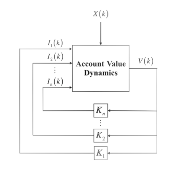
The problem formulation above is readily interpreted in terms classical feedback control theory. That is, we view as the state of a system with linear feedback and inputs corresponding to the investment levels for each of the gambles. That is, the -th input of the control signal is given by
with viewed as a feedback gain. Subsequently, the state for this stochastic system is updated via the equation
This type of feedback-control configuration is depicted in Figure 1; see [17] where this paradigm is pursued in much greater detail.
I-D Plan for Sections to Follow
Although limitations of the Kelly-based theory are mentioned in the existing literature, there is a paucity of specific examples illustrating the degree to which things can “go wrong.” To this end, Section 2 concentrates on approximation methods in the literature which are used to optimize the allocation vector . As shown in the sequel, the Taylor series are used to approximate the log-growth function, we see that the solution which is obtained may be either infeasible or lead to performance which is significantly lower than that of the true optimum. In addition, we show that approximate solutions may have a certain “inefficiency property” which is undesirable.
Although our examples to follow provide specific realizations of the “badness” which can occur, it should also be noted that a “remedy” is readily available. That is, some papers, for example, see [3] and [10], recognize that the log-growth problem is a concave program.
Hence, it is arguable that approximation methods are not needed because there are readily available commercial codes which efficiently solve the problem at hand; see [18] and [19]. At the time that some of the earlier papers were written, such codes were not readily available and authors either resorted to approximation or developed algorithms of their own; see [4].
In Section 3, a concern which is much more serious than approximation is addressed — the issue of wealth drawdown. Suffice it to say, the literature already recognizes that the Kelly gains which result, although being log-growth optimal, may be too aggressive in the short term; i.e., the wealth level may fall to unacceptably low levels along sample pathes. For this reason, as mentioned earlier, some authors resort to a so-called “fractional” betting scheme by scaling back the ; e.g., see [9] and [11]. Other authors resort to incorporation of constraints to reduce the drawdown effect; e.g., see [10]. After quantifying some of the negatives regarding drawdown, in Section 4, we describe some research directions which we feel are promising for mitigation of the drawdown problem. Finally, in Section 5, some conclusions are given and other directions of research are mentioned.
II Negatives Associated with Approximation
In order to obtain the optimal logarithmic growth rate above, as previously mentioned, one approach in the literature involves approximation — either a multivariate Taylor expansion to the log-growth function is used or is treated as a Geometric Brownian Motion and low order expansion terms are used; e.g., see [6], [12], [13], and [14]. The main objective in this section is to point out some “pitfalls” associated with approximate solution. While approximation-based closed-form solutions for the optimal provide a degree of insight into the risk-return tradeoffs, concrete examples do not appear in the literature which demonstrate scenarios where approximation methods lead to erroneous results. Suffice it to say, when the range of variation of can be large, the true optimum and associated logarithmic growth can differ considerably from its approximation.
II-A Example Involving Approximation
We consider the somewhat attractive gamble for which , with probability and with probability . We call this bet “attractive” in a central-limiting sense; i.e., since , repeated i.i.d. trials, will almost certainly lead to success. Now, according to [13], using the approximation
it is straightforward to see that the associated optimum investment fraction , call it , is given by
Note that this solution is not feasible because is assumed. Hence, to guarantee feasibility, a saturation function is introduced for the approximate solution above. Thus, the optimal approximate solution with saturation, call it , and the associated expected log-growth are as follows
where is a saturation function; i.e., for , ; for , and for , we have .
An alternative approach, for example, see [6] and [12], with being treated as a Geometric Brownian Motion with drift and variance . A subsequent Taylor approximation leads to approximate solution, call it , as
Similarly, it is infeasible with restriction so the saturation is required. Here, the associated optimal approximate solution, call it as , and the corresponding expected log-growth are given by
In contrast to the two approximate solutions above, the true optimum, as described in Section 1, is obtained by maximizing the expected logarithmic growth
which, by straightforward differentiation, leads to a feasible solution in and optimal growth given by
A summary of all three solutions is given in Figure 2. Ironically, the approximation-based results yields the minimum growth of rather than the desired maximum. Suffice it to say, the combination of approximation and saturation due to constraint violation can lead to significant error.
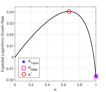
To quantify further, we convert the expected log-growth into an annualized rate of return using
Assuming daily betting, where is the time between bets in years, we take and then, the corresponding expected annualized rates of return are computed to be
In other words, the approximate betting schemes perform poorly compared to what is possible.
II-B More Realistic Example with Real Stock Data
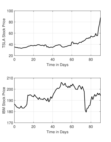
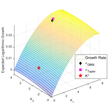
In this example, we further consider the problems associated with approximation by using an example involving real data for two stocks: Tesla Motors and IBM during the ninety-day period January 2, 2013 until May 13, 2013. We used the adjusted daily closing prices, see Figure 3, to estimate the joint probability mass function and carried out an in-sample constrained maximization of subject to the constraint , we obtain
That is, the optimum log-growth solution involves all funds invested in Tesla and no investment in IBM. Now, suppose instead that one computes the Taylor-based solutions; i.e.,
where is the second moment matrix for and is the covariance matrix for .
Note that the approximate solutions and are infeasible since the constraint is violated. The true optimum solution and approximate solutions along with and are seen in Figure 4.
Given the constraint violation for the Taylor and GBM solutions, one standard approach is to project these solutions onto the constraint satisfaction set. That is, we take
where is a projection function given by
for all nonnegative with not both . However, one should note that although the projection procedure provides a way for yielding a feasible solution, the projected solution may not be the optimal.
II-C Inefficiency of Approximate Solution
In this subsection, we point out another danger associated with the use of approximate solutions. The takeoff point is the following principle widely used in finance: If two investments have the same risk, the one with the smaller reward will be discarded and deemed to be “inefficient.” We claim that the use of either the approximation or might be inefficient. We now provide such an example using and note that the same example can be used for too. Indeed, we consider a random variable described as follows: Given , we have with probability and with probability . Using the Taylor approximation, as a function of reward level , a straightforward calculation yields
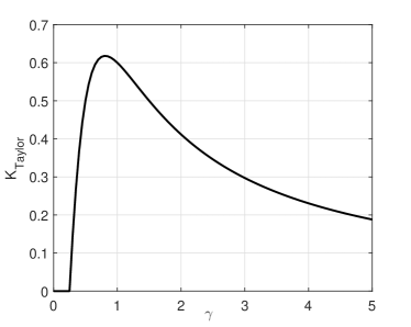
In order for to be efficient from an economic risk-taking point of view, it should have the following property: When , we require That is, if the bet associated with offers more reward with the same probabilities of success and failure as those for , a rational gambler should invest at least as much in the bet as the bet. We claim that the Taylor-based approximation scheme fails to satisfy this condition. To establish this claim, it suffices to show that can be negative with the in . Indeed, we calculate
and note that the denominator cannot vanish. Hence, we see for
which corresponds to the zero-crossing of the numerator. In the Figure 5, the plot of is given for . It is readily apparent that the claimed inefficiency occurs for parameter range
III Negatives Associated with Drawdown
As described in [10] and [16], control of drawdown, that is, control of the drops in wealth from peaks to subsequent lows, is one of great concern from a risk management perspective. In this section, we first demonstrate that Kelly betting often results in very poor drawdown performance. Then, we discuss some approaches for mitigating the drawdown problem within this framework. Along any sample path , the maximum percentage drawdown is defined as
In the sequel, we often drop the word “percentage” for expression simplicity.
As mentioned in Section 1, use of Kelly fraction may lead to a significant drawdown since it is too aggressive. To quantify see how bad the drawdown can be, consider betting times of single coin flipping gamble for which with probability and with probability , then it is easy to show that the probability of maximum drawdown greater than or equal to any fraction is given by
Now if we take and , using the optimal Kelly investment fraction It follows that there is a chance that maximum drawdown is over . That is, there is a large drawdown occurs with very high probability. A similar analysis using the Markov inequality also leads to the same conclusion.
III-A Control of Drawdown
To control the drawdown, one possible choice is to add probabilistic constraint to the optimization of log-growth; i.e., given and , consider the constraint
Alternatively, instead of using the probabilistic constraint above, we can use the expected maximum drawdown; i.e., given , consider the drawdown constraint as
We now revisit the example used in Section 2 with , with probability and with probability .
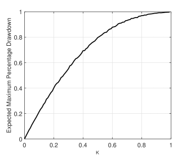
Using the optimum fraction already found, it is clear to see from Figure 6 that the corresponding expected maximum drawdown are
This shows that the approximation solution leads to an almost sure ruin. Now, suppose the gambler adds constraint . Then, based on Figure 6, it is clear to see that the optimal investment fraction reduces to
IV Research Directions Involving Drawdown
Further to the discussion of drawdown above, if the allocation vector is multi-dimensional, it would be desirable to have a convex drawdown constraint so that the log-growth optimization problem can be treated as concave program and can be solved in a very efficient way.
To this end, in this section we provide two conjectures involving convexity of the maximum drawdown.
For motivation, consider the single coin flipping example, it is clear from the monotonicity in Figure 6 that expected drawdown is increasing function in . Thus, for , the leads to an interval constraint for which is convex.
For two identical coins for which with probability and with probability for , a Monte Carlo simulation indicates that the constraint set of expected maximum drawdown defines a convex set; e.g., see Figure 7. This leads to the following conjecture.
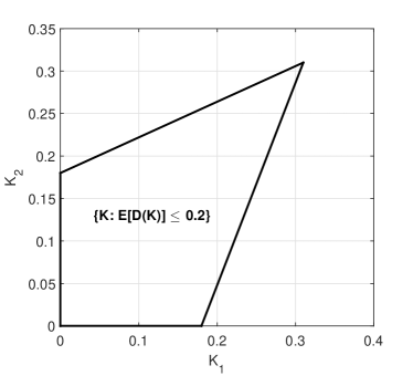
Conjecture 1: Given , the set for the expected maximum drawdown
is convex.
Instead of constraining expected maximum drawdown, we might consider the set for the probability that the maximum drawdown stays below some level . For the same two identical coins flipping example, Figure 8 shows that the drawdown constraint set is still convex. This leads to the following conjecture.
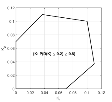
Conjecture 2: Given and , the set for the probability of maximum drawdown
is convex.
Although we have carried out several Monte Carlo simulations supporting these conjectures, in view of the fact that involving two coins, the question on the convexity is still the conjectures which may not be true for general case, we now introduce a surrogate for expected drawdown.
IV-A Surrogate for Expected Drawdown
First noting that
where
define complementary maximum drawdown. We consider this complementary drawdown as a surrogate and work with the surrogate constraint
Thus, the following lemma indicates that this complementary drawdown constraint defines a convex set.
Lemma IV.1
Given , the set
is convex.
Proof: Given , we have
Note that the function is concave in , using the fact that the minimum over an index collection of the concave functions is concave, it follows that is a concave function. Hence, the set
is convex.
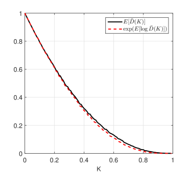
Remark: Since log function is concave, using Jensen’s inequality, we obtain
Now exponentiating on both sides, we obtain
To consider the tightness of this bound, we revisit the single coin flipping gamble again with probability and . Figure 9 provides a comparison between and obatined by using Monte Carlo simulation.
For this simple case, It is clear that is very close to . In other words, the surrogate complementary drawdown can be a drawdown candidate.
V Conclusion
In this paper, the focal point was some of the limitations associated with application the Kelly Criterion. By way of further research, in addition to the drawdown issues described in Section 3, another possibility involves modification of the feedback control scheme defining the investment. Perhaps use of other variables in the “controller” such as the drawdown itself would result in improved performance. More generally, it would be of interest to pursue the Kelly-based theory with other risk metrics such as the Sharpe Ratio, see [20], in play.
An important line of future research involves extension of existing results to problems involving with not assumed to be known.
For example, when the theory is applied in a stock-trading context instead of assuming is known, it would make sense to consider the use of an adaptive scheme to obtain a -vector which is time-varying; i.e., as nature of the market dynamics change, the investment function is correspondingly adjusted.
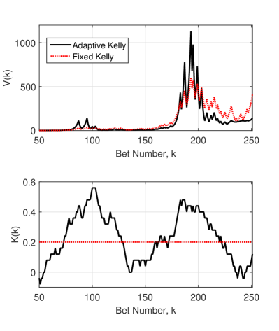
To provide a simple illustration how such an adaptive scheme might work, we consider the coin-flipping game described in Section 1 with initial account value and unknown underlying probability . Now, the bettor, not knowing observes outcomes and constructs a relative frequency estimate of using a sliding window of size . The first steps constitute the training period within which no betting is done, and then, for , the estimator is given by
Note that the estimator above is used for expressing that the number of winning bet. Now, using the estimator, we can obtain investment fraction
The results, summarized in Figure 10.
References
- [1] J. L. Kelly, “A New Interpretation of Information Rate,” Bell System Technical Journal, pp. 917-926, 1956.
- [2] N. H. Hakansson, “On Optimal Myopic Portfolio Policies With and Without Serial Correlation,” Journal of Business, vol. 44, pp. 324-334, 1972.
- [3] T. M. Cover, “An Algorithm For Maximizing Expected Log Investment Return,” IEEE Transactions on Information Theory, vol. 30, pp. 369-373, 1984.
- [4] T. M. Cover and J. A. Thomas, Elements of Information Theory, Wiley, 2012.
- [5] L. M. Rotando and E. O. Thorp, “The Kelly Criterion and the Stock Market,” The American Mathematical Monthly, vol. 99, pp. 922-931, 1992.
- [6] E. O. Thorp, “The Kelly Criterion in Blackjack Sports Betting and The Stock Market,” Handbook of Asset and Liability Management: Theory and Methodology, vol. 1, pp. 385-428. Elsevier Science, 2006.
- [7] P. Samuelson, “The “Fallacy” of Maximizing The Geometric Mean in Long Sequences of Investing or Gambling ,” Proceedings of the National Academy of Sciences, vol. 68, pp. 2493-2496, 1971.
- [8] S. Maslov and Y. C. Zhang, “Optimal Investment Strategy for Risky Assets,” International Journal of Theoretical and Applied Finance, vol. 1, pp. 377-387, 1998.
- [9] L. C. Maclean and W. T. Ziemba “Growth Versus Security Tradeoffs in Dynamic Investment Analysis,” Annals of Operations Research, vol. 85, pp. 193-227, 1999.
- [10] L. C. Maclean, R. Sanegre, Y. Zhao, and W. T. Ziemba “Capital Growth with Security,” Journal of Economic Dynamics and Control, vol. 28, pp. 937-954, 2004.
- [11] L. C. Maclean, E. O. Thorp, and W. T. Ziemba “Long-term Capital Growth: The Good and Bad Properties of The Kelly and Fractional Kelly Capital Growth Criteria,” Quantitative Finance, vol. 10, pp. 681-687, August-September, 2010.
- [12] J. K. Rising and A. J. Wyner, “Partial Kelly Portfolios and Shrinkage Estimators,” IEEE International Symposium on Information Theory Proceedings, pp. 1618-1622, 2012.
- [13] V. Nekrasov, “Kelly Criterion for Multivariate Portfolios: A Model-Free Approach,” Social Science Research Network Electronic Journal, 2014.
- [14] V. Nekrasov, Knowledge Rather Than Hope: A Book For Retail Investors and Mathematical Finance Students, Self-published by Author, 2014.
- [15] G. C. Calafiore and B. Monastero, “Triggering Long-Short Trades on Indexes,” International Journal of Trade, Economics and Finance, vol. 1, pp. 289-296, 2010.
- [16] S. Malepour and B. R. Barmish, “A Drawdown Formula for Stock Trading Via Linear Feedback in a Market Governed by Brownian Motion,” Proceedings of the European Control Conference, Zurich, Switzerland, pp. 87-92, July 2013.
- [17] B. R. Barmish and J. A. Primbs, “On a New Paradigm for Stock Trading Via a Model-Free Feedback Controller,” IEEE Transactions on Automatic Control, 2015, in press.
- [18] S. P. Boyd and L. Vandenberghe, Convex Optimization,, Cambridge University Press, 2004.
- [19] M. C. Grant and S. P. Boyd, “CVX: Matlab Software for Disciplined Convex Programming”, Ver 2.1, 2015.
- [20] W. F. Sharpe, “The Sharpe Ratio,” Journal of Portfolio Management, vol. 21, pp. 49-58, 1994.