Semantic 3D Reconstruction with Finite Element Bases

Abstract

We propose a novel framework for the discretisation of multi-label problems on arbitrary, continuous domains. Our work bridges the gap between general FEM discretisations, and labeling problems that arise in a variety of computer vision tasks, including for instance those derived from the generalised Potts model. Starting from the popular formulation of labeling as a convex relaxation by functional lifting, we show that FEM discretisation is valid for the most general case, where the regulariser is anisotropic and non-metric. While our findings are generic and applicable to different vision problems, we demonstrate their practical implementation in the context of semantic 3D reconstruction, where such regularisers have proved particularly beneficial. The proposed FEM approach leads to a smaller memory footprint as well as faster computation, and it constitutes a very simple way to enable variable, adaptive resolution within the same model.

1 Introduction

A number of computer vision tasks, such as segmentation, multiview reconstruction, stitching and inpainting, can be formulated as multi-label problems on continuous domains, by functional lifting [Pock et al.(2010)Pock, Cremers, Bischof, and Chambolle, Cremers et al.(2011)Cremers, Pock, Kolev, and Chambolle, Lellmann and Schnörr(2011), Chambolle et al.(2012)Chambolle, Cremers, and Pock, Nieuwenhuis et al.(2013)Nieuwenhuis, Töppe, and Cremers]. A recent example is semantic 3D reconstruction (e.g[Häne et al.(2013)Häne, Zach, Cohen, Angst, and Pollefeys, Blaha et al.(2016)Blaha, Vogel, Richard, Wegner, Pock, and Schindler]), which solves the following problem: Given a set of images of a scene, reconstruct both its 3D shape and a segmentation into semantic object classes. The task is particularly challenging, because the evidence is irregularly distributed in the 3D domain; but it also possesses a rich, anisotropic prior structure that can be exploited. Jointly reasoning about shape and class allows one to take into account class-specific shape priors (e.g, building walls should be smooth and vertical, and vice versa smooth, vertical surfaces are likely to be building walls), leading to improved reconstruction results. So far, models for the mentioned multi-label problems, and in particular for semantic 3D reconstruction, have been limited to axis-aligned discretisations. Unless the scenes are aligned with the coordinate axes, this leads to an unnecessarily large number of elements. Moreover, since the evidence is (inevitably) distributed unevenly in 3D, it also causes biased reconstructions. Thus, it is desirable to adapt the discretisation to the scene content (as often done for purely geometric surface reconstruction, e.g. [Labatut et al.(2007)Labatut, Pons, and Keriven]).

Our formulation makes it possible to employ a finer tesselation in regions that are likely to contain a surface, exploiting the fact that both high spatial resolution and high numerical precision are only required in those regions. Our discretisation scheme leads to a smaller memory footprint and faster computation, and it constitues a very simple technique to allow for arbitrary adaptive resolution levels within the same problem. I.e, we can refine or coarsen the discretisation as appropriate, to adapt to the scene to be reconstructed. While our scheme is applicable to a whole family of finite element bases, we investigate two particularly interesting cases: Lagrange (P1) and Raviart-Thomas elements of first order. We further show that the grid-based voxel discretisation is a special case of our P1 basis, such that minimum energy solutions of “identical” discretisations (same vertex set) are equivalent.

Figure 1: Semantic 3D model, estimated from aerial views with our FEM method.

2 Related Work

Since the seminal work [Curless and Levoy(1996)] volumetric reconstruction from image data has evolved remarkably [Kazhdan et al.(2006)Kazhdan, Bolitho, and Hoppe, Vogiatzis et al.(2007)Vogiatzis, Esteban, Torr, and Cipolla, Furukawa and Ponce(2010), Liu and Cooper(2010), Cremers and Kolev(2011), Kolev et al.(2012)Kolev, Brox, and Cremers, Kostrikov et al.(2014)Kostrikov, Horbert, and Leibe, Ulusoy et al.(2016)Ulusoy, Black, and Geiger]. Most methods use depth maps or 2.5D range scans for evidence [Zach et al.(2007)Zach, Pock, and Bischof, Zach(2008)], represent the scene via an indicator or signed distance function in the volumetric domain, and extract the surface as its zero level set, e.g, [Lorensen and Cline(1987), Treece(1999)].

Joint estimation of geometry and semantic labels, which had earlier been attempted only for single depth maps [Ladický et al.(2010)Ladický, Sturgess, Russell, Sengupta, Bastanlar, Clocksin, and Torr], has recently emerged as a powerful extension of volumetric 3D reconstruction from multiple views [Häne et al.(2013)Häne, Zach, Cohen, Angst, and Pollefeys, Bao et al.(2013)Bao, Chandraker, Lin, and Savarese, Kundu et al.(2014)Kundu, Li, Dellaert, Li, and Rehg, Savinov et al.(2015)Savinov, Ladický, Häne, and Pollefeys, Vineet et al.(2015)Vineet, Miksik, Lidegaard, Nießner, Golodetz, Prisacariu, Kähler, Murray, Izadi, Perez, and Torr, Blaha et al.(2016)Blaha, Vogel, Richard, Wegner, Pock, and Schindler, Ulusoy et al.(2017)Ulusoy, Black, and Geiger]. A common trait of these works is the integration of depth estimates and appearance-based labeling information from multiple images, with class-specific regularisation via shape priors.

Multi-label problems are in general NP-hard, but under certain conditions on the pairwise interactions, the original non-convex problem can be converted into a convex one via functional lifting and subsequent relaxation, e.g[Chambolle et al.(2012)Chambolle, Cremers, and Pock]. This construction was further extended to anisotropic (direction-dependent) regularisers [Strekalovskiy and Cremers(2011)]. Moreover, [Zach et al.(2014)Zach, Häne, and Pollefeys] also relaxed the requirement that the regulariser forms a metric on the label set, yet its construction can only be applied after discretisation [Lellmann and Schnörr(2011)]. In this paper, we consider the relaxation in its most general form [Zach et al.(2014)Zach, Häne, and Pollefeys], but are not restricted to it. The latter construction is also the basis to the model of [Häne et al.(2013)Häne, Zach, Cohen, Angst, and Pollefeys], whose energy model we adapt for our semantic 3D reconstruction method. Their voxel-based formulation can be seen as a special case of our discretisation scheme.

For (non-semantic) surface reconstruction, several authors prefer a data-dependent discretisation, normally a Delaunay tetrahedralisation of a 3D point cloud [Labatut et al.(2007)Labatut, Pons, and Keriven, Jancosek and Pajdla(2011), Vu et al.(2012)Vu, Labatut, Pons, and Keriven]. The occupancy states of the tetrahedra are found by discrete (binary) labeling, and the final surface is composed of the triangles that separate different labels. Loosely speaking, our proposed methodology can be seen either as an extension of [Häne et al.(2013)Häne, Zach, Cohen, Angst, and Pollefeys] to arbitrary simplex partitions of the domain; or as an extension of [Labatut et al.(2007)Labatut, Pons, and Keriven] to semantic (multi-label) reconstruction.

We note that regular voxel partitioning of the volume leads to a high memory consumption and computation time. Yet, we are essentially reconstructing a 2D manifold in 3D space, and this can be exploited to reduce run-time and memory footprint. [Kundu et al.(2014)Kundu, Li, Dellaert, Li, and Rehg] use an octree instead of equally sized voxels to adapt to the local density of the input data. [Blaha et al.(2016)Blaha, Vogel, Richard, Wegner, Pock, and Schindler] go one step further and propose an adaptive octree, where the discretisation is refined on-the-fly, during optimisation. In our framework the energy is independent of the discretisation, it can thus be combined directly with such an adaptive procedure.

Also volumetric fusion via signed distance functions [Newcombe et al.(2011)Newcombe, Izadi, Hilliges, Molyneaux, Kim, Davison, Kohli, Shotton, Hodges, and Fitzgibbon] benefits from irregular tesselations of 3D space, e.g, octrees [Steinbruecker et al.(2014)Steinbruecker, Sturm, and Cremers] or hashmaps [Nießner et al.(2013)Nießner, Zollhöfer, Izadi, and Stamminger]. In contrast to our work, these target real-time reconstruction and refrain from global optimisation, instead locally fusing depth maps. Their input normally is a densely sampled, overcomplete RGB-D video-stream, whereas we deal with noisy and incomplete inputs. To achieve high-quality reconstructions in our setting, we incorporate semantic information, leading to a multi-label problem.

Our work is based on the finite element method (FEM), e.g[Reddy(2005), Brezzi and Fortin(1991)]. Introduced by Ritz [Ritz(1909)] more than a century ago, and refined by Galerkin and Courant [Courant(1943)], FEM serves to numerically solve variational problems, by partitioning the domain into finite, parametrised elements. In computer vision FEM has been applied in the context of level-set methods [Weber et al.(2004)Weber, Blake, and Cipolla] and for Total Variation [Bartels(2012)]. To our knowledge, we are the first to apply it to multi-labeling.

3 Method

The multi-labeling problem [Chambolle et al.(2012)Chambolle, Cremers, and Pock, Strekalovskiy and Cremers(2011), Lellmann and Schnörr(2011), Zach et al.(2014)Zach, Häne, and Pollefeys] in the domain $\Omega\subset\mathbb{R}^{d}$ is defined by finding $m$ labeling functions $x^{i}:\Omega\rightarrow\{0,1\},i=1\ldots m$ as the solution of:

$$\inf_{x^{i}}\sum_{i=1}^{m}\int_{\Omega}\rho^{i}(z)x^{i}(z)\mathrm{d}z+J(x^{i}),\quad\textrm{s.\ t. }\sum_{i=1}^{m}x^{i}(z)=1\;\forall z\in\Omega,\vspace{-0.1cm}$$ (1)

where $\rho$ models the data term for a specific label at location $z\in\Omega$ and $J$ denotes a convex regularisation functional that enforces the spatial consistency of the labels. One prominent example is to chose $J:=\|{\cdot}\|{{}_{2}}$, known as Total Variation, which penalises the perimeter of the individual regions [Chambolle et al.(2012)Chambolle, Cremers, and Pock, Nieuwenhuis et al.(2013)Nieuwenhuis, Töppe, and Cremers]. Note that in the two-label case (Potts model), this relaxation is exact after thresholding with any threshold from the open unit interval [Chambolle et al.(2012)Chambolle, Cremers, and Pock]. Although we are ultimately interested in non-metric regularisation, we start with the continuous, anisotropic model [Strekalovskiy and Cremers(2011)], and postpone the extension to the non-metric case to Sec. 3.5.

3.1 Convex Relaxation

The continuous model allows for an anisotropic regulariser in $J$: label transitions can be penalised on the area of the shared surface, as well as on the surface normal direction. This is achieved with problem-specific 1-homogeneous functions that emerge from convex sets, so called Wulff-shapes. A relaxation of $x^{i}(z)\in\{0,1\}$ to $x^{i}(z)\in[0,1]$ then leads to a convex energy, which can be written as the following saddle point problem, with primal functions $x$ and dual functions $\lambda$:

$$\min_{x^{i}}\max_{\lambda^{i}}\sum_{i}\!\!\!\int_{\Omega}\!\!\!\!\rho^{i}\!(z)x^{i}(z)\!\!+\!\!\langle x^{i}(z),\nabla\!\cdot\!\lambda^{i}(z)\rangle\mathrm{d}z,\;\;\textrm{s.t. }\lambda^{i}(z)\!-\!\lambda^{j}(z)\in W^{ij}\!\!,\sum_{i=1}^{m}\!x^{i}(z)\!\!=\!\!1,x^{i}(z)\!\geq\!0.\vspace{-0.1cm}$$ (2)

The constraints have to be fulfilled for all $z\in\Omega$. In addition to the primal variables $x^{i}$, we have introduced the dual vector-field $\lambda^{i}:\mathbb{R}^{d}\rightarrow\mathbb{R}^{d}$, whose pairwise differences are constrained to lie in the convex sets (Wulff-shapes) $W^{ij}$. By letting these shapes take an anisotropic form, one can then encode scene structure, e.g[Strekalovskiy and Cremers(2011), Häne et al.(2013)Häne, Zach, Cohen, Angst, and Pollefeys]. For our problem we demand Neumann conditions at the boundary of $\Omega$, i.e$\langle\lambda^{i},\nu\rangle=0,\forall z\in\partial\Omega$, because the scene will continue beyond our domain ($\nu$ is the normal of the domain boundary $\partial\Omega$).

3.2 Finite Element Spaces

Here, we can only informally introduce the basic idea of FEM and explain its suitability for problems of the form (2). We refer to textbooks [Larson and Bengzon(2013), Brezzi and Fortin(1991), Durán(2008)] for a deeper and formal treatment.

One way to solve  (2) is to approximate it at a finite number of regular grid points, using finite differences. FEM instead searches for a solution in a finite-dimensional vector space; this trial space is a subspace of the space in which the exact solution is defined. To that end, one chooses a suitable basis for the trial space, with basis functions of finite support, as well as an appropriate test function space. FEM methods then find approximate solutions to variational problems by identifying the element from the trial space that is orthogonal to all functions of the test function space. For our saddle-point problem, we can instead identify the trial space with our primal function space and the test space with its dual counterpart. Now, we can apply the same principles, and after discretisation our solution corresponds to the continuous solution defined by the respective basis. As (2) is already a relaxation of the original problem (1), we do not present an analysis of convergence at this point. Instead, the reader is referred to [Bartels(2012)] for an introduction to this somewhat involved topic.

In order to choose a space with good approximation properties and suitable basis functions, we tesselate our domain into simplices. More formally, we define $M\!=\!\{F,V,S\}$ to be a simplex mesh with vertices $v\!\in\!V,v\!\in\!\mathbb{R}^{d}$, faces $f\!\in\!F$ defined by $d$, and simplices $s\!\in\!S$, defined by $d\!+\!1$ vertices that partition $\Omega$: $\cup_{k}s_{k}=\Omega,s_{l}\cap s_{k}\!=\!f_{l,k}\!\in\!F$ – i.etwo adjacent simplices share only a single face. In this work, for a specific set of vertices $V$, we select M to be the corresponding Delaunay tetrahedralisation of $\Omega$ and only consider explicit bases. In particular, we focus on the Lagrangian (P1) basis, which we use in the following to derive our framework; and on the Raviart-Thomas (RT) basis. Details for the latter are given in the supplementary material. The main difference between them is that P1 leads to piecewise linear solutions, which must be thresholded, while RT leads to a constant labeling function per simplex, similar to discrete MAP solutions on CRFs. We note that constant labeling can lead to artefacts, such that the adaptiveness of the FEM model becomes even more important.

The idea of both derivations is similar: (i) select a basis for our primal (P1) or dual (RT) variable set, (ii) find a suitable form via the divergence theorem and Fenchel duality, (iii) extend to the non-metric case, following a principle we term ”label mass preservation”.

3.3 Lagrange Elements

The Lagrange $\textrm{P}^{k}(M)$ basis functions describe a conforming polynomial basis of order $k\!+\!1$ on our simplex mesh $M$, i.eits elements belong to the Hilbert space of differentiable function with finite Lebesgue measure on the domain $\Omega$: $\textrm{P}^{k}(M)\subset H^{1}(\Omega):=\{p\in L^{2}(\Omega),\nabla p\in(L^{2}(\Omega)^{d})\}$. We are interested in the Lagrange basis of first order, $\textrm{P}^{1}(M)$:

$$P^{1}(M)\!\!:=\!\{\!p\!:\Omega\!\rightarrow\!\mathbb{R}|p\!\in\!C(\Omega),\,p(x)\!:=\!\sum_{s\in S}c_{s}^{\!\mathsf{T}}x+d_{s},c_{s}\!\in\!\mathbb{R}^{d},d_{s}\!\in\!\mathbb{R},\textrm{ if }x\!\in\!s\textrm{ and }0\textrm{ else}\}.\vspace{-.125cm}$$ (3)

We construct our linear basis with functions that are defined for each vertex $v$ of a simplex $s$ and can be described in local form with barycentric coordinates:

$$p^{1}_{s,v}(x):=\alpha_{v}\;\textrm{with }x=\sum_{v\in s}\alpha_{v}v,\;\sum_{v\in s}\alpha_{v}=1,\;\alpha_{v}\geq 0\quad\textrm{if}\;x\in s\;\textrm{and}\;0\;\textrm{else}.\vspace{-0.125cm}$$ (4)

In each simplex, one can define a scalar field $\phi_{s}(x)\in\mathbb{R}$ and compute a gradient in this basis that will be constant per simplex $s$ (cf. Fig. 2):

$$\phi_{s}(x):=\sum_{v\in s}\phi_{v}p^{1}_{s,v}\;\textrm{ and }\nabla\phi_{s}=\sum_{v\in s}\phi_{v}J_{v},\vspace{-0.125cm}$$ (5)

with coefficients $\phi_{v}\in\mathbb{R}$. $J_{v}\in\mathbb{R}^{d}$ denotes a vector that is normal to the face $f_{v}$ opposite node $v$, has length $\frac{|f_{v}|}{|s|d}$, and points towards the simplex centre. $|f_{v}|$ denotes the area of the face $f_{v}$, and $|s|$ the volume of the simplex $s$ (cfFig. 2 and supplementary material).

Figure 2: Left: Illustration of P1 basis function shape. Middle: Scalar field defined as a convex combination of basis coefficients. Right: Gradient definition in a simplex (5).

3.4 Discretisation

To apply our Lagrange basis to (2) we first make use of the divergence theorem:

$$\int_{\Omega}\langle x^{i}(z),\nabla\!\cdot\!\lambda^{i}(z)\rangle\mathrm{d}z=\;\int_{\Omega}\langle\nabla x^{i}(z),\lambda^{i}(z)\rangle\mathrm{d}z-\underbrace{\int_{\partial\Omega}\langle\nu(z),\lambda^{i}(z)\rangle\mathrm{d}z}_{=0}.\vspace{-0.25cm}$$ (6)

The latter summand vanishes by our choice of $\lambda$. Our approach for a discretisation in the Lagrange basis is to choose the labeling function $x^{i}\in P^{1}(M)$. This implies that our dual space consists of constant vector-fields per simplex: $\lambda^{i}_{s}\in\mathbb{R}^{d}$. To fulfill the constraint set in (2) we have to verify that, per simplex, the $\lambda^{i}_{s}$ lie in the respective Wulff-shape. The simplex constraints on the $x^{i}$ have to be modeled per vertex. According to (4), the labeling functions are convex combinations of their values at the vertices and thus stay within the simplex.

We also have to convert the continuous data costs $\rho^{i}$ into a cost per vertex $\rho^{i}_{v}$, which can be achieved by convolving the continuous cost with the respective basis function: $\rho^{i}_{v}:=\int_{\Omega}\sum_{s\in\mathcal{N}(v)}\phi_{s}(x)\rho^{i}(x)\mathrm{d}x$. In practice, the integral can be computed by sampling $\rho$. Integrating the right hand side in (6) over the simplex $s$ leads to a weighting with its volume $|s|$ and the energy (2) in the discrete setting becomes:

$$\min_{x^{i}}\max_{\lambda^{i}}\sum_{v,i}\rho^{i}_{v}x_{v}^{i}\!+\!\sum_{s,i}|s|\langle\nabla x^{i},\lambda_{s}^{i}\rangle\;\;\textrm{s.t. }(\!\lambda_{s}^{i}-\lambda_{s}^{j}\!)\!\in\!W^{ij}\;\forall i\!<\!j,\;s\in S,\sum_{i=1}^{m}\!x_{v}^{i}\!\!=\!\!1,\;x_{v}^{i}\!\geq\!0\;\forall v\!\in\!V.\vspace{-0.1cm}$$ (7)

3.5 Non-metric extension

To start with, we note that a non-metric model does not exist in the continuous case [Maggi(2012)] and our extension works only after the discretisation into the FEM basis. Please refer to the supplementary material for an in-depth discussion. Note that our label set of semantic classes does not have a natural order (in contrast to, e.g, stereo depth or denoised brightness); and also the direction-dependent regulariser is unordered and does not induce a metric cost. To allow for non-metric regularisation we transform the constraint set ($\lambda^{i}-\lambda^{j}\in W^{ij}$), by introducing auxiliary variables $z^{ij}$ and Lagrange multipliers $y^{ij}$, and use Fenchel-Duality:

$$\max_{\lambda_{s}^{i},z_{s}^{ij}}\min_{y_{s}^{ij}}\sum_{i<j}\langle(\lambda_{s}^{i}-\lambda_{s}^{j})-z^{ij},y_{s}^{ij}\rangle-\delta_{W^{ij}}(z_{s}^{ij})=\max_{\lambda_{s}^{i}}\min_{y_{s}^{ij}}\sum_{i<j}-\langle(\lambda_{s}^{i}-\lambda_{s}^{j}),y_{s}^{ij}\rangle+||y_{s}^{ij}||_{W^{ij}}.\vspace{-0.1cm}$$ (8)

The dual functions of the indicator functions for the convex sets $W^{ij}$ are 1-homogeneous, of the form $||\cdot||_{W^{ij}}\!:=\!\sup_{w\in W^{ij}}w^{\!\mathsf{T}}\cdot$. Recall that our label costs are not metric: $\forall i\!<\!j\!<\!k:|y^{ij}|_{W^{ij}}+|y^{jk}|_{W^{jk}}\geq|y^{ik}|_{W^{ik}}$, does not hold. It was shown [Zach et al.(2014)Zach, Häne, and Pollefeys] that a regulariser of the form (8) transforms any non-metric cost to the metric case. Figure 3 shows an example. Here, an expensive transition between labels 0 and 2 will be replaced by two cheaper transitions 0–1 and 1–2. To prevent this, we replace the $y^{ij}$ with direction dependent variables $x^{ij}$: We rearrange (8) and combine the first summand with the regulariser from (7) to arrive at the following equations (for now ignoring $|s|$):

$$\sum_{s}\sum_{i}\langle\nabla x^{i},\lambda_{s}^{i}\rangle-\sum_{i}\langle\lambda_{s}^{i},\sum_{j\neq i}\left(y_{s}^{ij}[i<j]-y_{s}^{ji}[i>j]\right)\rangle,\vspace{-0.1cm}$$

with $[\cdot]$ denoting Iverson brackets. Let $x^{ij}:=[y^{ij}]_{+}$ and $x^{ji}:=[-y^{ji}]_{+}$, where $[\cdot]_{+}:=\max(0,\cdot)$. Expanding the gradient (5) we get, per simplex $s$,

$$\sum_{i}\sum_{v\in s}\lambda^{i}_{s}x_{v}^{i}([J_{v}]_{+}-[-J_{v}]_{+})-\langle\lambda_{s}^{i},\sum_{j:i\neq j}(x^{ij}-x^{ji})\rangle,\vspace{-0.14cm}$$ (9)

which we analyse further to achieve non-metric costs. It was observed in [Zach et al.(2014)Zach, Häne, and Pollefeys] that the $x^{ij}\in\mathbb{R}^{d}$ can be interpreted as encoding the “label mass” that transitions from label $i$ to label $j$ in a specific direction. Positivity constraints (by definition) on the $x^{ij}$ avoid the transport of negative label mass. To anchor transport of mass on the actual mass of label $i$ present at a vertex, we introduce the variables $x^{ii}$ for the mass that remains at label $i$, and split the above constraints into two separate sets with the help of additional dual variables $\theta$:

$$\lambda^{i}_{s}(\sum_{v\in s}x_{v}^{i}[J_{v}]_{+}-\sum_{j}x_{s}^{ij})+\theta^{i}_{s}(\sum_{v\in s}x_{v}^{i}[-J_{v}]_{+}-\sum_{j}x_{s}^{ji})+\sum_{i,j}\delta_{\geq 0}(x_{s}^{ij}).\vspace{-0.075cm}$$ (10)

Figure 3: Left: Without our non-metric extension, optimisation w.r.t(7) can lower transition costs by inserting another label (here 1 between 0 and 2). Right: A solution is to split the gradients of the indicator functions and use direction-dependent variables $x^{ij}$.

Note that this construction is only possible because our elements (simplices) are of strictly positive volume, in contrast to zero sets in $\Omega$ w.r.tthe Lebesgue measure. Finally, we can write down our discrete energy in the Lagrange basis defined on the simplex mesh $M$:

$$\begin{split}\min_{x^{i},x^{ij}}\max_{\lambda^{i},\theta^{i}}&\sum_{v\in V}\sum_{i}\rho^{i}_{v}x_{v}^{i}+\delta_{\Delta}(x_{v}^{i})+\sum_{i<j}\sum_{s\in S}|s|||x_{s}^{ij}-x_{s}^{ji}||_{W^{ij}}+\\ &\sum_{s}\sum_{i}\theta^{i}_{s}(\sum_{v\in s}x_{v}^{i}[-J_{v}]_{+}-\sum_{j}x_{s}^{ji})+\sum_{s}\sum_{i}\lambda^{i}_{s}(\sum_{v\in s}x_{v}^{i}[J_{v}]_{+}-\sum_{j}x_{s}^{ij})+\sum_{i,j}\delta_{\geq 0}(x_{s}^{ij}),\end{split}\vspace{-0.075cm}$$ (11)

where we have moved the weighting with $|s|$ from the constraint set to the regulariser, and denote by $\delta_{\Delta}(\cdot)$ the indicator function of the unit simplex.

4 Semantic Reconstruction Model

A prime application scenario for our FEM multi-label energy model (11) is 3D semantic reconstruction. In particular, we focus on an urban scenario and let our labeling functions encode freespace ($i=1$), building wall, roof, vegetation or ground. Objects that are not explicitly modeled are collected in an extra clutter class. We define the data cost $\rho$ at a 3D-point $x\in\Omega$ as in [Häne et al.(2013)Häne, Zach, Cohen, Angst, and Pollefeys]: project $x$ into the camera views $c\in\mathcal{C}$, and retrieve the corresponding depth $\hat{d}_{c}(x)$ and class likelihoods $\sigma_{c}^{i}(x)$ from the image space. The $\sigma^{i}$ are obtained from a MultiBoost classifier. For the depth we look at the difference between the actual distance $d_{c}(x)$ to the camera and the observed depth: $d(x,c):=d_{c}(x)-\hat{d}_{c}(x)$. For the freespace label we always set the cost to 0, for $i\neq 1$ we define:

$$\rho^{i}(x)\!:=\!\sum_{c\in\mathcal{C}}\!\sigma_{c}^{i}(x)[(k\!-1\!)\epsilon\leq d(x,c)\leq k\epsilon]+\beta[|d(x,c)|\leq k\epsilon]\operatorname*{sign}(d(x,c)).\vspace{-0.075cm}$$ (12)

This model assumes independence of the per-pixel observations, and exponentially distributed inlier noise in the depthmaps, bounded by a parameter $k\epsilon$ (k=3 in practice). It is essentially a continuous version of [Häne et al.(2013)Häne, Zach, Cohen, Angst, and Pollefeys], see that paper for details. The parameter $\epsilon$ sets a lower bound for the minimal height of the simplices in the tesselation, and thus defines the target resolution. The discretisation of the data cost involves a convolution with the respective basis functions, which can be approximated via sampling. Please refer to the supplementary material for details. The Wulff-shapes $W^{ij}$ in (11) are given as the Minkowski sum of the $L_{2}$-Ball, $B^{2}_{\kappa^{ij}}:=\{x\in\mathbb{R}^{d}|\|x\|_{2}\leq\kappa^{ij}\}$ and an anisotropic shape $\Psi^{ij}$: $W^{ij}:=\Psi^{ij}\oplus B^{2}_{\kappa^{ij}}$. In the isotropic part, $\kappa^{ij}$ contains the neighbourhood statistics of the classes. The anisotropic part $\Psi^{ij}$ models the likelihood of a transition between classes $i$ and $j$ in a certain direction. Fig. 4 (a,b) shows an example. For our case we prefer flat, horizontal surfaces at the following label transitions: ground-freespace, ground-building, building-roof, ground-vegetation and roof-freespace. A second prior prefers vertical boundaries for the transitions building-freespace and building-vegetation. More details on the exact form can be found in [Häne et al.(2013)Häne, Zach, Cohen, Angst, and Pollefeys].

Figure 4: (a): Wulff-shape (red) with isolines. (b): Minkowski sum of two Wulff-shapes. (c): Simplices are split after inserting new vertices (blue) close to the surface (green). Right: Initialisation of vertices after refinement. (d): Finite differences on a regular grid ([Häne et al.(2013)Häne, Zach, Cohen, Angst, and Pollefeys]) only cover constraints in green areas, the P1 basis covers all of the domain $\Omega$.

The energy (11) is already in primal-dual form, such that we can apply the minimisation scheme of [Chambolle and Pock(2011)], with pre-conditioning [Pock and Chambolle(2011)]. That numerical scheme requires us to project onto shapes that are Minkowski sums of convex sets. In our case, the sets are simple and the projection onto each shape can be performed in closed form. We employ a Dykstra-like projection scheme [Boyle and Dykstra(1986)], which avoids storing additional variables and proves remarkably efficient, see supplementary material. We also project the labeling functions $x^{i}$ directly onto the unit simplex [Wang and Carreira-Perpiñán(2013)]. In order to extract the transition surface, we employ a variant of marching tetrahedra (triangles) [Treece(1999)], using the isolevel at $0.5$ for each label.

We conclude with two interesting remarks. First, note that a tesselation with a regular grid [Häne et al.(2013)Häne, Zach, Cohen, Angst, and Pollefeys] can be seen as a simplified version of our discretisation in the $P^{1}$ Lagrange basis. In Fig. 4d we consider the 2D case of the regular grid used in [Häne et al.(2013)Häne, Zach, Cohen, Angst, and Pollefeys]. Here, variables are defined at voxel level. In its dual graph, the vertex set consists of the corners of the primal grid cubes, leading to shifted indicator variables. Per vertex the data term is mainly influenced from the cost in its Voronoi area. Similarly, [Häne et al.(2013)Häne, Zach, Cohen, Angst, and Pollefeys] evaluates the data cost at grid centers, approximately corresponding to integration within the respective Voronoi-area of grid cell. Furthermore, taking finite differences in this regular case corresponds to verifying constraints for only one of the two triangles (Fig. 4d). The supplementary material includes a more formal analysis.

Second, our formulation is adaptive, in the sense of [Blaha et al.(2016)Blaha, Vogel, Richard, Wegner, Pock, and Schindler]: Hierarchical refinement of the tesselation can only decrease our energy. Hence, our scheme is applicable when refining the model on-the-fly. We again must defer a formal proof to the supplementary material and give an intuitive, visual explanation in Fig. 4c . Assume that $(x^{*},\lambda^{*},\theta^{*})$ is an optimal solution for a certain triplet $M=\{F,V,S\}$. Then a refined tesselation $\hat{M}=\{\hat{F},\hat{V},\hat{S}\}$ can be found by introducing additional vertices, i.e$V\subset\hat{V}$ (ideally on the label transition surfaces). To define a new set of simplices, we demand that no faces are flipped, $\forall\hat{s}\in\hat{S},\exists s\in S$ with $\hat{s}\cap s=\hat{s}$. Then one can find a new variable set and data cost $\hat{\rho}$ with the same energy: We initialise the new variables from the continuous solution at the respective location, and find new $\rho_{\hat{v}}$ by integration. Subsequent minimisation in the refined mesh can only decrease the energy. The argument works in both ways: Vertices that have the same solution as their adjacent neighbors can be removed without changing the energy. For now we stick to this simple scheme, future work might explore more sophisticated ideas, e.galong the lines of [Grinspun et al.(2002)Grinspun, Krysl, and Schröder].

5 Evaluation

Before we present results on challenging real 3D data we evaluate our method in 2D on a synthetic dataset. All results are obtained with a multi-core implementation, on a 12-core, 3.5 GHz machine with 64GB RAM. For clarity, we only present the Lagrange discretisation. We refer to the supplementary material for an evaluation of the Raviart-Thomas discretisation.

Input Data. We create a synthetic 2D scene composed of 4 labels: free space, building, ground and roof, surrounded by 17 virtual cameras. To replace depth maps and class-likelihood images, we extract 2D points on the boundary “surface” and assign ground truth label costs to each point. For the evaluation in 3D, we use three real-world aerial mapping data sets. Our method requires two types of input data: depthmaps and pixel-wise class probabilities (cfSec. 4). Moreover, we build a control mesh $M$ around the initially predicted surface, to facilitate our FEM discretisation. Ideally, the control mesh enwraps the true surface, using a finer meshing close to it. We densely evaluate the data cost at the vertices of a regular data cost grid and let each control vertex accumulate the cost of its nearest neighbours in that grid, to approximate an integration over its Voronoi cell.

Figure 5: Left: Synthetic 2D scene, colors indicate ground (gray), building (red) and roof (yellow). Middle: Control mesh. Right: Example reconstruction.

overall acc. [%]	Tetra	Octree	MB
Scene 1	84.0	83.9	82.5
Scene 2	92.5	92.8	89

Table 1: Quantitative comparison with octree model [Blaha et al.(2016)Blaha, Vogel, Richard, Wegner, Pock, and Schindler] and MultiBoost input data.

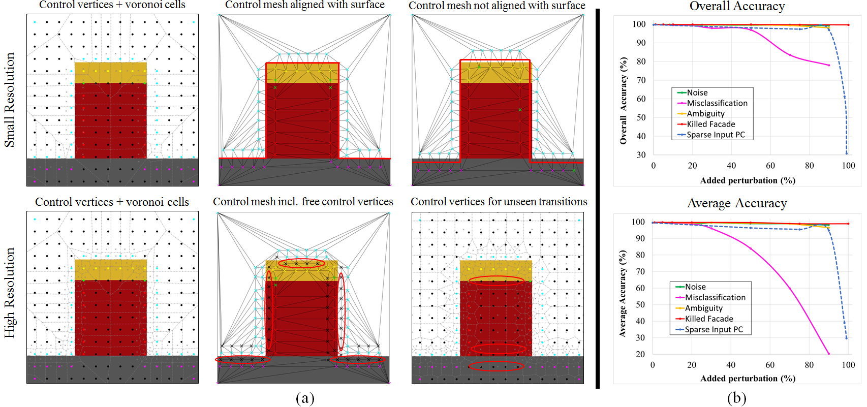
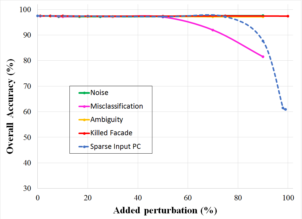
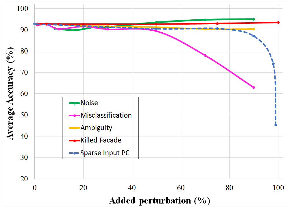
2D Lagrange results. Fig. 5 illustrates the result we obtain in a perfect setting. The original 2D image serves as ground truth for our quantitative evaluation. In this baseline setting, our method achieves $99.8\%$ of overall accuracy and $99.7\%$ of average accuracy, confirming the soundness of our Lagrange discretisation. In order to evaluate how our model behaves in a more realistic setting, we conduct a series of experiments where we incrementally add different types of perturbations. Our algorithm is tested against: (i) noise in the initial 2D point cloud, respectively depth maps, (ii) wrong class probabilities and (iii) ambiguous class probabilities of random subsets, (iv) missing data, e.gdeleting part of a facade to simulate unobserved areas, (v) sparsity of the initial point cloud. Fig. 6b illustrates the influence of defective inputs. Under reasonable assumptions on the magnitude of the investigated perturbations, we do not observe a significant loss in accuracy. The reconstruction quality starts to decrease if more than half of the input data is misclassified or if the input point cloud is excessively sparse, meaning that $>$50% of the input is wrong or nonexistent. Average accuracy is naturally more sensitive, due to the larger relative error in small classes.

Influence of the control mesh. Recall from (12) that the data cost of a control vertex $v\!\in\!V$ is approximately equal to an integral of $\rho$ over its respective Voronoi area (cfFig. 6a, left). Therefore, but also because of the sign change in (12), vertices close to the surface receive small cost values and are mainly steered by the regulariser, i.ethese vertices realise a smooth surface. On the other hand, vertices that integrate only over areas with positive or negative sign determine the inside/outside decision, but are more or less agnostic about the exact location of the surface. We conclude that a sufficient amount of control vertices should lie within the band $[\hat{d}-3\epsilon;\hat{d}+3\epsilon]$ defined by the truncation of the cost function around the observed depth $\hat{d}$ (cf(12) and [Häne et al.(2013)Häne, Zach, Cohen, Angst, and Pollefeys]). Ideally control vertices are equally distributed along each line-of-sight in front and behind the putative match (cfFig. 6a, middle column). Undersampling within the near-band can lead to smooth, but inaccurate results (cfFig. 6a, top right). Unobserved transitions, e.gbuilding-ground or roof-building, can also lead to problems if the affected simplices are too large. To mitigate the effect, we add a few vertices (e.g, a sparse regular grid) on top of the control mesh (cfFig. 6a, bottom row). Finally, oversampling each line-of-sight in order to increase the resolution of the control mesh is not recommended, the right spacing is determined by the noise level and $\epsilon$ and $k$, chosen in (12).

To conclude, it is an important advantage of the FEM framework that additional vertices can be inserted as required, without changing the energy. In future work we will use this flexibility to develop smarter control meshes, possibly as a function of the local noise level.

Figure 6: (a) Illustration of the control mesh foundation. Dots represent values of the datacost grid and crosses the control vertices. Voronoi cells of the control vertices are depicted with dashed grey lines and the control mesh with a solid black line. Colors indicate ground (purple), building (red), roof (yellow), free space (cyan) and no datacost (black). (b) Quantitative evaluation of Lagrange FEM method w.r.tdifferent degradations of the input data.

3D Lagrange results. To test our algorithm on real world data, we focus on a dataset from the city of Enschede. Complementary results for other datasets are shown in the supplementary material. As baseline we use [Blaha et al.(2016)Blaha, Vogel, Richard, Wegner, Pock, and Schindler], the current state-of-the-art in large-scale semantic 3D reconstruction. Due to the lack of 3D ground truth, we follow their evaluation protocol and back-project subsets of the 3D reconstruction to image space, where it is compared to a manual segmentation. As can be seen in Fig. 7 and Tab. 5, the two results are similar in terms of quantitative correctness. We note that measuring labeling accuracy in the 2D projection does not consider the geometric quality of the reconstruction within regions of a single label.

Figs. 1 and 7 show city-modelling results obtained from (nadir and oblique) aerial images. Visually, our models are crisper and less “clay-like”. Compared to axis-aligned discretisation schemes, e.g[Häne et al.(2013)Häne, Zach, Cohen, Angst, and Pollefeys, Blaha et al.(2016)Blaha, Vogel, Richard, Wegner, Pock, and Schindler], our method appears to better represent surfaces not aligned with the coordinate axis, and exhibit reduced grid aliasing. Both effects are consistent with the main strength of the FEM framework, to adapt the size and the orientation of the volume elements to the data. Small tetrahedra, and vertices that coincide with accurate 3D points on surface discontinuities, favour sharp surface details and crease edges (e.g, substructures on roofs). Faces that follow the data points rather than arbitrary grid directions mitigate aliasing on surfaces not aligned with the coordinate axes (e.g, building walls). The freedom of a local control mesh unleashes the power of the regulariser in regions where the evidence is weak or ambiguous (e.g, roads, weakly textured building parts).

As already mentioned, our FEM framework can be readily combined with on-the-fly adaptive computation, as used in the baseline [Blaha et al.(2016)Blaha, Vogel, Richard, Wegner, Pock, and Schindler]. Compared to their voxel/octree model, adaptive refinement is straight-forward, due to the flexibility of the FEM framework, which allows for the introduction of arbitrary new vertices. As a preliminary proof-of-concept, we have tested the naive refinement scheme described in Sec. 4. We execute three refinement steps, where we repeatedly reconstruct the scene and subsequently refine simplices that contain surface transitions, while lowering $\epsilon$ by half. Compared to computing everything at the final resolution, this already yields substantial savings of 89–97% in memory and 82–93% in computation time, without any loss in accuracy. Targetting $\epsilon\geq\frac{1}{\sqrt{3}}$ (measured w.r.ta bounding box of 256 units), the runtimes for the tested scenes are 1h04m–1h47m and memory consumption is 573–764 MB, on a single machine.

Figure 7: Quantitative evaluation of Scene 1 from Enschede. Left: One of the input images. Middle left: Semantic 3D model. Middle right: Back-projected labels overlayed on the image. Right: Error map, misclassified pixels are marked in red.

6 Conclusion

We have proposed a novel framework for the discretisation of multi-label problems, and have shown that, in the context of semantic 3D reconstruction, the increased flexibility of our scheme allows one to better adapt the discretisation to the data at hand. Our basic idea is generic and not limited to semantic 3D reconstruction or the specific class of regularisers. We would like to explore other applications where it may be useful to abandon grid discretisations and move to a decomposition into simplices.

Acknowledgements: Audrey Richard was supported by SNF grant $200021\_157101$. Christoph Vogel and Thomas Pock acknowledge support from the ERC starting grant 640156, ’HOMOVIS’.

Supplementary Material

This document provides supplementary information to support the main paper. It is structured as follows: Sec. A gives more information about the data and pre-processing used in our experiments, not mentioned in the paper due to lack of space. We hope that the added details will help readers to better appreciate the experimental results. In Sec. B we show complementary results obtained with the proposed Lagrange FEM method on other datasets, as well as the full large-scale reconstruction of the city of Enschede. Sec. C contains technical details and formal proofs that had to be omitted in the paper. Finally, Sec. D discusses our formalism for the case of the Raviart-Thomas basis (instead of Lagrange P1), leading to piecewise constant labels. We also show results in 2D and 3D and a comparison to those obtained with the Lagrange basis.

Appendix A Input Data

For our real-world experiments, we start from aerial images, cfFig. 8. To mitigate foreshortening and occlusion, images are acquired in a Maltese cross configuration, with four oblique views in addition to the classical nadir view. We orient the images with VisualSFM [Wu(2011)], create depth maps from neighbouring views with Semi-global Matching [Hirschmüller(2008), Bradski(2000)], and predict pixel-wise class-conditional probabilities with a MultiBoost classifier [Benbouzid et al.(2012)Benbouzid, Busa-Fekete, Casagrande, Collin, and Kégl]. The classifier is trained on a few hand-labeled images, using the same features as [Blaha et al.(2016)Blaha, Vogel, Richard, Wegner, Pock, and Schindler]: raw RGB-intensities in a $5\times 5$ window, and $19$ geometry features (height, normal direction, anisotropy of structure tensor, etc) derived from the depth map.

Figure 8: Input data. Left: aerial input images for one position (four oblique views to the north, east, south, west, and a nadir image). Middle: oriented image block. Right: depth map and class probabilities (visualised by maximum-likelihood labels).

Appendix B Additional Visualizations

We have tested our semantic reconstruction method on several (synthetic) 2D and (real) 3D datasets. Here we provide additional examples to give the reader an impression of the variety of cases tested in our evaluation. We apply the same prior models as for our 3D reconstructions. We prefer flat, horizontal structures in the model for the following label transitions: ground-freespace, ground-building, building-roof and roof-freespace. The second prior applies to the transition building-freespace and prefers vertical boundaries. Fig. 9 shows examples for different degradations of the synthetic input (many more cases were tested).

Figure 9: Example scenes of our 2D data set and results obtained with our Lagrange FEM method. Left: Data term at vertices of the control mesh. Colors for the data cost indicate: free space/empty space (cyan), building (red), ground (pink), roof (yellow), occupied space (green) and no data cost (black). Middle: Semantic 2D model. Right: Classification result, misclassified pixels are depicted in red.

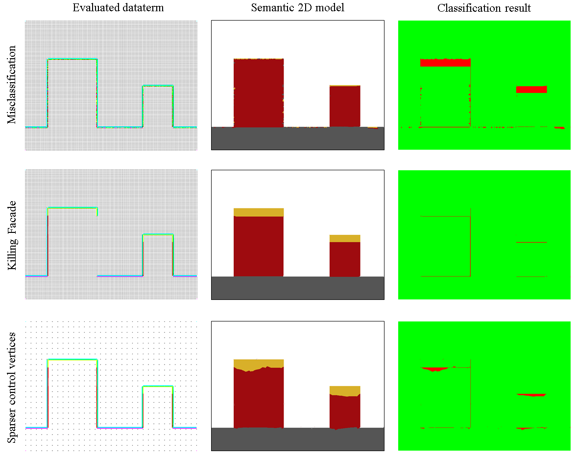
In the top row, we simulate imperfect classifier input by adding noise to the semantic class likelihoods. In our experience, the method is still able to reconstruct the geometry quite well, but sometimes assigns the wrong label. A closer inspection reveals that, locally, the roof and building classes are confused in locations where the class likelihoods are significantly wrong. The global geometry and labels in other regions remain unaffected. The second row gives an example of missing input data, a frequent situation in the real world, due to occlusions and constraints on camera placement. Fortunately, missing data does not seem to greatly challenge our method. In fact, our method is specifically designed to work well for these cases and complete the outline, relying on the prior assumptions about pairwise class transitions and class-specific local shape. In the last row we utilise only a sparse control mesh, even near the surface. The method can still recover the geometry, but struggles to determine the correct semantic labeling near the (unobserved) roof-to-building transition. The adaptive version of our method is designed to avoid exactly that case. It refines the control mesh near the predicted transitions, effectively increasing the resolution at the most promising locations.

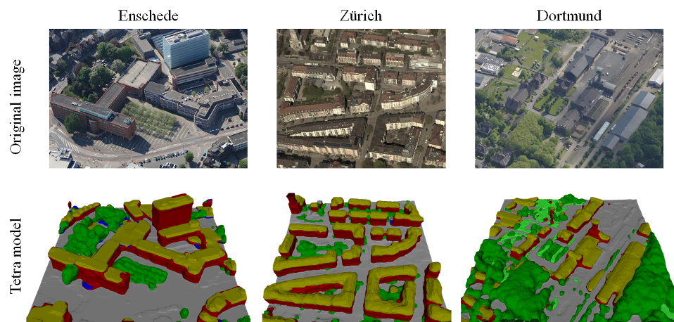
Fig. 10 shows city models obtained from two additional aerial datasets (Zürich, Switzerland and Dortmund, Germany), and a further patch from Enschede. These results qualitatively illustrate that our method works for different image sets and architectural layouts.

Figure 10: Additional datasets. First row: Original aerial images. Second row: Semantic 3D models obtained with the Lagrange FEM method for Enschede (left), Zürich (middle) and Dortmund (right). For the latter, light green denotes an additional class grass and agricultural fields.

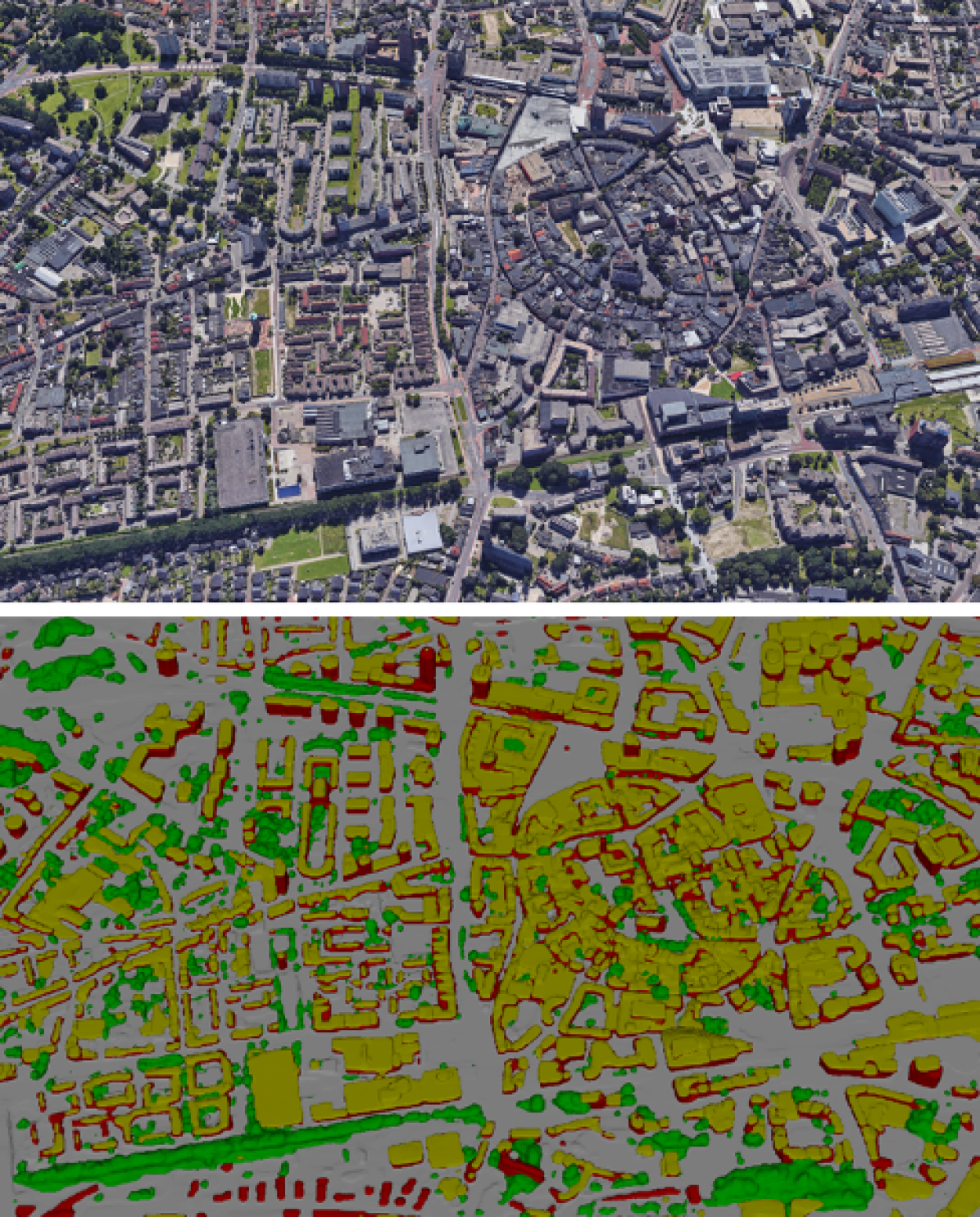
Finally, we show the complete semantic 3D reconstruction of Enschede. Fig. 11 shows the model rendered in an oblique view, together with the corresponding viewpoint in Google Earth, to illustrate its accuracy and high level-of-detail.

Figure 11: Large-scale semantic 3D reconstruction of Enschede (Netherlands), computed from aerial images with our Lagrange FEM method. Top: View from Google Earth (not used during reconstruction). Bottom: Our model from matching viewpoint.

Appendix C Proofs

In this section we give the technical proofs promised in the main paper, as well as further details about the optimisation. We start with a discussion of the extension to non-metric energies, and its consequences on the equivalence of continuous and discrete models.

C.1 Non-metric priors: continuous vs. discrete

The main message of this section is that a non-metric model does not exist in the continuous view, unless one imposes additional constraints on the function spaces. We briefly explain why: Let’s look at the transition boundary between two labels $i$ and $k$. Without additional constraints, one can always introduce a zero set with label $j$ between the two, i.e, a set with Lebesgue measure $0$ in the domain space. If the transition costs are not metric, then the cost for the label pair $\{i,k\}$ is potentially higher than the sum of the costs for $\{i,j\}$ and $\{j,k\}$. Inserting the zero set will avoid that extra cost and the energy will be under-estimated. In other words, let $S$ be a segmentation of $\Omega$ into regions $S^{i}$ and $S^{k}$, labeled with $i$ and $k$ respectively. Assume further that their costs do not fulfill the triangle inequality w.r.t another label $j$. Then one can find a sequence of segmentations $S^{n}:=\{S_{i}^{n},S_{j}^{n},S_{k}^{n}\}$ with $\displaystyle S=\lim_{n\to\infty}(S^{n})$: the label $j$ disappears in the limit, such that $\displaystyle\lim_{n\to\infty}\inf E(S^{n})<E(S)$. Hence, metric transition costs are a necessary condition for the lower semi-continuity of the energy functional. Methods that try to resolve the issue with additional constraints on the function space, for instance by demanding Lipshitz continuity of the labeling functions, are an active research area, e.g[Bretin and Masnou(2017)], but are beyond the scope of this work.

The above conceptual problem does have consequences for a practical implementation: Any discretisation of the domain will ultimately consist only of a finite number of elements of measurable ($>0$) volume. Thus, the label $j$ in the example will not disappear completely from the solution, and the computed energy matches the solution. In practice, one can simply prescribe a minimum edge length in the tesselation, since one cannot refine infinitely. Note that this also constrains the Lipshitz constant of the labeling functions; they are restricted to values between $0$ and $1$, such that the Lipshitz constant of functions $f\in P^{1}(M)$ defined on the mesh $M=\{V,F,S\}$ is bounded by $\min_{v\in s,s\in S}||J_{v}||$, cf (13). Because we utilise a Delaunay triangulation/tetrahedralisation of the domain and also limit the minimal dihedral angle, a further constraint on the edge length implies a bound on the Lipshitz constant. Note also, our analysis implies that a discrete solution in the non-metric setting does not have a continuous counterpart, and consequently investigations of the limiting case, i.e, convergence analysis after infinite refinement of the tesselation, are futile.

C.2 Gradient in the Lagrange basis

We show that gradients of functions in the P1 (Lagrange) basis are constant per simplex $s$ and given by:

$$\nabla\phi_{s}=\sum_{v\in s}\phi_{v}J_{v}$$ (13)

Here, the coefficients $\phi_{v}\in\mathbb{R}$ and $J_{v}\in\mathbb{R}^{d}$ denote a vector of length $\frac{|f_{v}|}{|s|d}$, normal to the face $f_{v}$ opposite to vertex $v$, and pointing inwards towards the center of the simplex. Recall that $|f_{v}|$ is the area of face $f_{v}$ and $|s|$ is the volume of simplex $s$.

The gradient can be obtained with basic algebra. First, notice that the gradient of $\phi_{s}$ in (13) has to fulfill $\langle v_{l}-v_{k},\nabla\phi_{s}\rangle=\phi_{v_{l}}-\phi_{v_{k}}$, meaning that integration along the edge leads to the respective change in $\phi_{s}$. After collecting a sufficient number of linear equations of this form, one can directly solve the resulting linear system. Since $J_{v}$ is, by definition, orthogonal to all edges that do not involve vertex $v$, we arrive at (13).

Formally, we pick one vertex $v$ of simplex $s$ and compile for $l=1\ldots d$ ($v_{l}\neq v$) equations of the form $\langle v_{l}-v,\nabla\phi_{s}\rangle=\phi_{v_{l}}-\phi_{v}$. By construction, $\langle J_{v_{l}},v_{k}-v\rangle=\delta_{k=l}$. The vector $J_{v_{l}}$ is normal to face $f_{v_{l}}$. The scalar product of the edge $(v_{l}-v)$ and the normal is the ”height” within the simplex, so with the chosen scaling of $J_{v_{l}}$ we have $\langle J_{v_{l}},v_{l}-v_{k}\rangle=1$ for any $k\neq l$.

Thus multiplying each side of our equation system by a matrix with the vectors $J_{v_{l}},l=1\ldots d$ as columns leads to: $\nabla\phi_{s}=\sum_{l}J_{v_{l}}(\phi_{v_{l}}-\phi_{v})$. If we can show that $\sum_{l}J_{v_{l}}=-J_{v}$, then we arrive at the desired expression (13). For $v_{k},v_{j}\neq v$, $\langle\sum_{l}J_{v_{l}},v_{j}-v_{k}\rangle=\langle J_{v_{l}},v_{j}\rangle-\langle J_{v_{k}},v_{k}\rangle=0$ and $\langle\sum_{l}J_{v_{l}},v_{k}-v\rangle=\langle J_{v_{k}},v_{k}-v\rangle=1$. All equations are also fulfilled by $J_{v}$ in place of $\sum_{l}J_{v_{l}}$, which concludes the proof.

C.3 Data Term for Lagrange basis

We again start from the ideas in the main paper. We have to convert the continuous data costs $\rho^{i}$ into discrete form (in a practical implementation, “continuous” means that the cost can be evaluated at any $z\in\Omega$). In our basis representation, we can get discrete cost values for the basis elements by convolving the continuous cost with the respective basis function. For simplicity, we consider the P1 basis function here. Thus, we seek a cost per vertex $\rho^{i}_{v}$. In detail we obtain:

$$\int_{\Omega}x^{i}(z)\rho^{i}(z)\mathrm{d}z= \sum_{s}\int_{s}x_{s}^{i}(z)\rho^{i}(z)\mathrm{d}z=\sum_{s}\int_{s}\sum_{v\in s}\phi_{v}p^{1}_{s,v}(z)\rho^{i}(z)\mathrm{d}z=$$

$$\sum_{v\in V}\phi_{v}\underbrace{\left(\sum_{s\in N(v)}\int_{s}p^{1}_{s,v}(z)\rho^{i}(z)\mathrm{d}z\right)}_{:=\rho_{v}^{i}}=\langle\rho^{i}_{v},x^{i}_{v}\rangle.$$ (14)

To numerically compute $\rho^{i}_{v}$, we sample $\rho^{i}$ at a finite number of locations $z\in\Omega$. For each $z$ we determine into which simplex $s$ it falls, and accumulate the contributions of $\rho^{i}(z)$ over all $i=1\ldots m$, weighted by their barycentric coordinates. The final step is to scale $\rho^{i}_{v}$ by $\sum_{s\in N(v)}\frac{|s|}{d}$ and divide by the sum of weights assigned to vertex $v$. In other words, we compute the sample mean and scale it by the area covered by the vertex. In our current implementation $\rho$ is sampled at regular grid points, without importance sampling. This simple strategy is indeed very similar to the method employed in [Häne et al.(2013)Häne, Zach, Cohen, Angst, and Pollefeys, Blaha et al.(2016)Blaha, Vogel, Richard, Wegner, Pock, and Schindler]. There, the data cost is evaluated on a regular grid, by reprojecting grid vertices into each image, computing the data term, and adding its respective contribution to the grid location. Such a “per-voxel accumulation” is equivalent to integrating the data cost within the respective Voronoi-area of a vertex in the dual grid: the latter is proportional to the number of regular samples that fall into a Voronoi-cell and therefore have the respective vertex as nearest neighbour. Hence, summing the individual contributions directly corresponds to integrating the data term within the Voronoi region.

C.4 Grid vs. P1

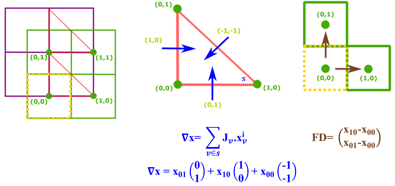
Here, we detail why the grid-based version with finite differences (corresponding to [Häne et al.(2013)Häne, Zach, Cohen, Angst, and Pollefeys]) can be seen as an approximation of our proposed FEM discretisation with P1 basis elements, if the vertices (cells) are aligned in a regular grid. Without loss of generality we consider a grid of edge length $1$, and note that in this case the gradient for a function $f:\Omega\subset\mathbb{R}^{d}\rightarrow\mathbb{R}$ at a grid point x, evaluated with forward differences becomes:

$$\nabla f=(f_{x+e_{1}}-f_{x},\ldots,f_{x+e_{d}}-f_{x})^{\!\mathsf{T}}=\sum_{i}e_{i}f_{x+e_{i}}-\sum_{i}e_{i}f_{x}=\sum f_{x+e_{i}}J_{x+e_{i}}+f_{x}J_{x},$$ (15)

with $e_{i}$ the unit vector in direction $i$. We have used the identity $e_{i}=J_{x+e_{i}}$, according to the definition in Sec. C.2, and obtain the last equality from $\sum_{l}J_{v_{l}}=-J_{v}$, cfSec. C.2. This is exactly the formula for the gradient of the corresponding P1 function in the simplex defined by the vertices $\{x,x+e_{i}\}_{i=1}^{d}$. Accordingly, if implemented as finite differences, the constraints on the dual vector field $\lambda$, see Eq. (2) from the paper, are only checked within the respective simplex, but not in the whole domain (1/2 of the domain in 2D; 1/6 in 3D). Note also that, with grid-aligned vertices, the simplex in question cannot be part of a partition of $\Omega\subset\mathbb{R}^{d}$, unless $d\leq 2$: edges of adjacent faces would intersect.

Fig. 12 illustrates the specific case with $d=2$. On the left, the regular grid (green) and the triangle (simplex, red). Grid centers correspond to vertices in the (triangle-)mesh. The grid corresponds to the discretisation used in [Häne et al.(2013)Häne, Zach, Cohen, Angst, and Pollefeys], whereas the simplex mesh is used in this paper. The gradient of the lower left triangle for the simplex mesh corresponds exactly to the one computed via forward differences as shown in (15). Consequently, discretisation via finite differences is a special case of our method, where the elements are layed out on a regular grid, and the constraints are tested only in the upper right triangle (in the 2D case).

Figure 12: Left: Grid (green) and simplex mesh (red) cover the same domain, but are offset against each other. Grid centers correspond to vertex positions. The gradient in a triangle (middle) corresponds to the gradient computed with forward differences (right).

C.5 Adaptiveness

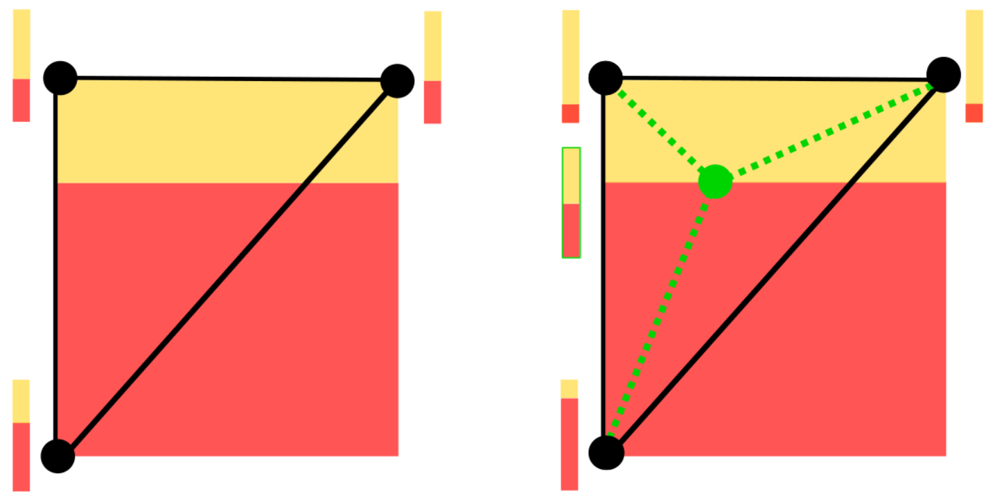
We have stated in the paper that our formulation is adaptive, in the sense that a hierarchical refinement of the tesselation can only decrease the energy. We have also explained a way to find the refined tesselation of $\Omega$, by introducing additional vertices and splitting simplices $s$, such that no faces $f\in F$ are flipped; and we have put forward a procedure to initialise the new variables. Here, we formally prove that the described scheme is sound.

Let $(x^{*},\lambda^{*},\theta^{*})$ be the solution for a triplet $M=\{F,V,S\}$. And let $\hat{M}=\{\hat{F},\hat{V},\hat{S}\}$ be the refined mesh with $V\subset\hat{V}$ and $\forall\hat{s}\in\hat{S},\exists s\in S$ with $\hat{s}\cap s=\hat{s}$. Furthermore, we define the sets $\bar{V}=\hat{V}\setminus V$ and $\bar{S}=\hat{S}\setminus S$ to denote newly introduced vertices and simplices. Our construction works by induction, i.ewe introduce one vertex $v$ at a time. The vertex is assumed to lie in simplex $s\in S$, $s=\{v_{k}\}_{k=1}^{d+1}$, which is split into simplices $\{\bar{s}_{k}\}_{k=1}^{d+1}$ with $\bar{s}_{k}\cap\bar{s}_{l}=\emptyset,\forall k\neq l$. By definition, vertex $\bar{v}$ has the barycentric coordinates $\frac{|\bar{s}_{k}|}{|s|}$, i.e$\bar{v}=\sum_{k=1}^{d+1}\frac{|\bar{s}_{k}|}{|s|}v_{k}$.

We initialize the labeling variables at new vertices $\bar{v}\in\bar{V}$ via barycentric interpolation: $x^{i}_{\bar{v}}=\sum_{v_{k}\in s}\frac{|\bar{s}_{k}|}{|s|}x^{i}_{v_{k}}$. Dual variables of the new simplices $\bar{s}_{k}$, and also the transition variables $x^{ij}$, are simply copied from their enclosing simplex $s$: $\lambda^{i}_{\bar{s}_{k}}:=\lambda^{i}_{s}$, $\theta^{i}_{\bar{s}_{k}}:=\theta^{i}_{s}$ and $x^{ij}_{\bar{s}_{k}}:=x^{ij}_{s}$. The data terms at the new vertex $\bar{v}$, as well as at the other vertices $v_{k}$ of simplex $s$, are (re)computed following (C.3), see also Fig. 13. We call the new variables $\bar{x},\bar{\lambda},\bar{\theta}$ and claim that $E_{M}(x^{*},\lambda^{*},\theta^{*})=E_{\hat{M}}(\bar{x},\bar{\lambda},\bar{\theta})$ and that $\bar{x},\bar{\lambda},\bar{\theta}$ is feasible. The latter is trivially the case (cfEq. (11) from the paper); transition variables remain positive by construction, the newly introduced labeling variables still fulfill the simplex constraints, and they induce the same gradients in the new simplices as in the parent simplex. The same applies for the cost of the regulariser in the new simplices: $\sum_{i<j}|s|||x_{s}^{ij}-x_{s}^{ji}||_{W^{ij}}=\sum_{i<j}\sum_{\bar{s}_{k}\in s}|\bar{s}_{k}|||x_{\bar{s}_{k}}^{ij}-x_{\bar{s}_{k}}^{ji}||_{W^{ij}}$. More interesting is the data cost. We introduce the notation $\rho_{v,s}:=\int_{s}p^{1}_{s,v}(z)\rho^{i}(z)\mathrm{d}z$ for the data cost at vertex $v$, originating from the integral over simplex $s$. By induction, we need to only verify the following equality for simplex $s$, which is split into $\{\bar{s}_{k}\}_{k=1}^{d+1}$:

$$\begin{split}\sum_{k}x^{i}_{v_{k}}\rho_{v_{k},s}=\sum_{k}x^{i}_{v_{k}}\sum_{j\neq k}\rho_{v_{k},\bar{s}_{j}}+\sum_{j}x^{i}_{\bar{v}}\rho_{\bar{v},\bar{s}_{j}}=\sum_{k}x^{i}_{v_{k}}\sum_{j\neq k}\rho_{v_{k},\bar{s}_{j}}+\frac{|\bar{s}_{k}|}{|s|}\sum_{j}x^{i}_{v_{k}}\rho_{v,\bar{s}_{j}}\end{split}$$ (16)

Recall we have ”old” vertices $v_{k}$, $s=\{v_{k}\}_{k=1}^{d+1}$ and a new vertex $\bar{v}$. According to (16), we must verify:

$$\rho_{v_{k},s}\!=\!\sum_{j\neq k}\rho_{v_{k},\bar{s}_{j}}\!+\!\frac{|\bar{s}_{k}|}{|s|}\sum_{j}\rho_{v,\bar{s}_{j}}\!\Leftrightarrow\!\int_{s}\!\rho(z)p^{1}_{s,v_{k}}(z)\mathrm{d}z\!=\!\!\int_{s}\!\rho(z)\sum_{j\neq k}p^{1}_{\bar{s_{j}},v_{k}}(z)\!+\!\!\frac{|\bar{s}_{k}|}{|s|}\sum_{j}p^{1}_{\bar{s}_{j},v}(z)\mathrm{d}z.$$ (17)

It is sufficient to show

$$p^{1}_{s,v_{k}}(z)=\sum_{j\neq k}p^{1}_{\bar{s_{j}},v_{k}}(z)+\frac{|\bar{s}_{k}|}{|s|}\sum_{j}p^{1}_{\bar{s}_{j},v}(z)\;\;\forall z\in s.$$ (18)

The right hand side represents a linear function for each $\{\bar{s}_{k}\}_{k=1}^{d+1}$. We can check if both sides agree on $d+1$ points in each simplex, which is easy to verify. The locations we check – substitute $z$ on both sides of Eq. (18) – are $\{v_{k}\}_{k=1}^{d+1}$ and $v$. These are the defining vertices of the $d+1$ simplices $\{\bar{s}_{k}\}_{k=1}^{d+1}$. Left and right hand side vanish, except for $v$ and $v_{k}$. Finally, we get $\frac{|\bar{s}_{k}|}{|s|}$ for $v$ and $1$ for $v_{k}$ on both sides.

In our adaptive version, we directly follow the proof and split simplices with the introduction of a single new vertex. We emphasise again that this splitting schedule is merely a proof of concept. The FEM discretisation allows for more sophisticated refinement schemes, e.g, along the lines of [Grinspun et al.(2002)Grinspun, Krysl, and Schröder], or flipping edges according to the energy functional, etc.

Figure 13: Updated data term after adding a new vertex.

C.6 Optimisation

The energy (11) from the paper is given in primal-dual form, optimisation with existing tools is straight-forward. We apply the minimisation scheme of [Chambolle and Pock(2011)], with pre-conditioning [Pock and Chambolle(2011)]. Internally, that algorithm however requires the projection onto the Wulff-shapes $W^{ij}$, which is slightly more involved.

C.6.1 Proxmap for the Minkowski sum of convex sets

Recall that, per label pair $\{i,j\}$, our Wulff-shapes are of the form $W^{ij}:=\Psi^{ij}\oplus B^{2}_{\kappa^{ij}}$. They are the Minkowski sum of two simple convex sets. Recall that the $\Psi^{ij}$ encode the direction dependent likelihood of a certain label transition. In our case, all Wulff-shapes permit a closed form projection scheme, such that we solve the following sub-problem as proximal step, independently per simplex $s$:

$$\operatorname*{arg\,min}_{x^{ij},x^{ji}}\frac{1}{2}||x^{ij}-\overline{x^{ij}}||^{2}+\frac{1}{2}||x^{ji}-\overline{x^{ji}}||^{2}+\!\!\!\!\!\!\sup_{w\in\Psi^{ij}\oplus B^{2}_{\kappa^{ij}}}\!\!\!w^{\!\mathsf{T}}(x^{ij}-x^{ji})+\iota_{\geq 0}(x^{ij})+\iota_{\geq 0}(x^{ji}).$$ (19)

For the following derivation we rename the two sets $W_{1}:=\Psi^{ij}$ and $W_{2}:=B^{2}_{\kappa^{ij}}$. In order to decouple the argument within the regulariser, we introduce auxiliary variables $\{y_{k},z_{k}\}_{k=0}^{2}$ and additional Lagrange multipliers $\{\mu_{k},\lambda_{k}\}_{k=0}^{2}$, and replace $x^{ij}$ and $x^{ji}$ respectively:

$$\begin{split}\min_{x^{ij},x^{ji},y_{k},z_{k}}\,\,\,\max_{\mu_{k},\lambda_{k}}&\frac{1}{2}||x^{ij}-\overline{x^{ij}}||^{2}+\frac{1}{2}||x^{ji}-\overline{x^{ji}}||^{2}+\\ \!\!\!\!\!\!\sum_{k\in\{1,2\}}\!\sup_{w\in W_{k}}&w^{\!\mathsf{T}}(y_{k}-z_{k})+\iota_{\geq 0}(y_{0})+\iota_{\geq 0}(z_{0})-\sum_{k=0}^{2}\lambda_{k}^{\!\mathsf{T}}(x^{ij}-y_{k})-\mu_{k}^{\!\mathsf{T}}(x^{ji}-z_{k}).\end{split}$$ (20)

Optimality w.r.t$x^{ij},x^{ji}$ implies:

$$x^{ij}=\overline{x^{ij}}+\sum_{k=0}^{2}\lambda_{k}\;\;\textrm{and}\;\;x^{ji}=\overline{x^{ji}}+\sum_{k=0}^{2}\mu_{k},$$ (21)

which, after reinserting into (20), leads to:

$$\begin{split}\min_{y_{k},z_{k}}\max_{\mu_{k},\lambda_{k}}&\frac{-1}{2}||\sum_{k=0}^{2}\lambda_{k}-\overline{x^{ij}}||^{2}+\frac{-1}{2}||\sum_{k=0}^{2}\mu_{k}-\overline{x^{ji}}||^{2}+\\ \sup_{w_{1}\in W_{1},w_{2}\in W_{2}}&w_{1}^{\!\mathsf{T}}(y_{1}-z_{1})+w_{2}^{\!\mathsf{T}}(y_{2}-z_{2})+\iota_{\geq 0}(y_{0})+\iota_{\geq 0}(z_{0})+\sum_{k=0}^{2}\lambda_{k}^{\!\mathsf{T}}y_{k}+\mu_{k}^{\!\mathsf{T}}z_{k}\;.\end{split}$$ (22)

Applying Fenchel-duality yields:

$$\begin{split}\max_{\mu_{k},\lambda_{k}}\min_{z_{k}}&\frac{-1}{2}||\sum_{k=0}^{2}\lambda_{k}-\overline{x^{ij}}||^{2}+\frac{-1}{2}||\sum_{k=0}^{2}\mu_{k}-\overline{x^{ji}}||^{2}\\ &-\iota_{W_{1}}(-\lambda_{1})-\iota_{W_{2}}(-\lambda_{2})-\iota_{\leq 0}(-\lambda_{0})-\iota_{\leq 0}(-\mu_{0})+\sum_{k=1}^{2}(\lambda_{k}+\mu_{k})^{\!\mathsf{T}}z_{k}.\end{split}$$ (23)

The latter summand requires $\lambda_{1}=-\mu_{1}$ and $\lambda_{2}=-\mu_{2}$:

$$\min_{\mu_{0},\lambda_{k}}\frac{1}{2}||\sum_{k=0}^{2}\lambda_{k}\!-\!\overline{x^{ij}}||^{2}\!+\!\frac{1}{2}||\sum_{k=1}^{2}\lambda_{k}\!+\!\overline{x^{ji}}\!-\!\mu_{0}||^{2}\!+\!\iota_{W_{1}}(\!-\lambda_{1})\!+\!\iota_{W_{2}}(\!-\lambda_{2})\!+\!\iota_{\geq 0}(\lambda_{0})\!+\!\iota_{\geq 0}(\mu_{0}).$$ (24)

In this last form, we can apply a few iterations of block coordinate descent on the dual variables and recover the update for $x^{ij},x^{ji}$ from (21).

Appendix D Raviart-Thomas basis

D.1 Methodology

In this section, we show how to discretise the convex relaxation, Eq. (2) from the paper, for the case of the Raviart-Thomas basis. For convenience, we restate the energy:

$$\min_{x^{i}}\max_{\lambda^{i}}\sum_{i}\!\!\!\int_{\Omega}\!\!\rho^{i}\!(z)x^{i}\!(z)\!\!+\!\!\langle x^{i}\!(z),\nabla\!\cdot\!\lambda^{i}\!(z)\rangle\mathrm{d}z,\;\;\textrm{s.t. }\lambda^{i}\!(z)\!-\!\lambda^{j}\!(z)\in W^{ij}\!,\sum_{i=1}^{m}\!x^{i}\!(z)\!\!=\!\!1,x^{i}\!(z)\!\geq\!0.$$ (25)

The Raviart-Thomas basis is chosen as a strong contrast to the (preferred) Lagrange basis. With Raviart-Thomas functions, we model the dual functions $\lambda$ in (25), within our trial space. The Raviart-Thomas $\textrm{RT}^{k}(M)$ basis functions describe a $div$-conforming polynomial basis of order $k\!+\!1$, i.ethe divergence of the modeled vector field is continuous across simplices. We again discretise on a simplex mesh $M=\{F,V,S\}$ with vertices $v\in V,v\in\mathbb{R}^{d}$; faces $f\in F$ defined by $d$ vertices; and simplices $s\in S$ defined by $d+1$ vertices, which partition $\Omega$: $\cup_{k}s_{k}=\Omega,s_{l}\cap s_{k}=f_{k,l}\in F$.

$$RT^{0}(M):=\{p:\Omega\rightarrow\mathbb{R}^{d}|\phi(x):=\sum_{s\in S}\phi_{s}(x)\textrm{ with }\phi_{s}(x):=c_{s}x+d_{s},c_{s}\!\in\!\mathbb{R},d_{s}\!\in\!\mathbb{R}^{d},$$

$$\quad\textrm{ if }x\!\in\!s\textrm{ and }0\textrm{ else},\textrm{and }\phi_{s}(x)\textrm{ is continuous for }x\in f_{v}(s)\textrm{ in direction }\nu^{s}_{f_{v}}\}.$$ (26)

Here, we have used $\nu^{s}_{f_{v}}$ to denote the (outward-pointing) normal of face $f_{v}$ of simplex $s$. By convention the face $f_{v}$ is located opposite the vertex $v$. We construct our linear basis with functions that are defined for each face $f_{v}$ in a simplex $s$, and can be described in a local form as:

$$\phi^{0}_{s,v}(x):=(x-v)\frac{|f_{v}|}{|s|d}\quad\textrm{if}\;x\in s\;\textrm{and}\;0\;\textrm{else},$$

where we again let $|f_{v}|$ denote the area of the face and $|s|$ the volume of the simplex. Let $\nu^{s}_{f_{v}}$ be the normal of face $f_{v}$ in simplex $s$, then the basis functions fulfill:

$$\langle\phi^{0}_{s,u}(x),\nu^{s}_{f_{v}}\rangle:=[u=v]\;\forall x\in f_{v},$$ (27)

with $[\cdot]$ denoting the Iverson bracket.

These basis functions make up the global function space by enforcing a consistent orientation. For each face $f$ we can distinguish its two adjacent simplices $s^{+}$ and $s^{-}$, by analysing the scalar product of the vector $\mathbf{1}$ and the normal $\nu^{s\pm}_{f}$ of the shared face $f$ (by convention again pointing outwards of the respective simplex). W.l.o.g., we define $\textrm{si}_{{f}}^{{s^{\pm}}}:=\operatorname*{sign}\langle\nu^{s^{\pm}}_{f};\mathbf{1}\rangle$, i.e$s_{f}^{+}\nu^{s^{+}}_{f}=s_{f}^{-}\nu^{s^{-}}_{f}$. The global basis functions per face $f_{v}$ are then given by:

$$\phi^{0}_{s,v}:=\begin{cases}\textrm{si}_{{f_{v}}}^{{s}}(x-v)\frac{|f_{v}|}{|s|d}\quad&\textrm{if}\;x\in s\\ 0&\textrm{else}.\end{cases}$$ (28)

In each simplex, our vector-field $\phi_{s}(x)\in\mathbb{R}^{d}$ can then be defined in the following manner, with coefficients $\phi_{f_{v}}\in\mathbb{R}$:

$$\phi_{s}(x):=\sum_{v\in s}\phi_{f_{v}}\phi^{0}_{s,v}(x).$$

By construction, cf(27),(28), the vector-field is continuous along a face $x\in f$ in direction of the face normal $\nu_{f}$ (of arbitrary, but fixed orientation), i.efor neighbouring faces $s^{+}$ and $s^{-}$ we have:

$$\langle\phi_{s^{\pm}}(x),\nu_{f}\rangle=\textrm{si}_{{f}}^{{s^{\pm}}}\langle x-v^{\pm},\nu_{f}\rangle\frac{|f|}{|s^{\pm}|d}\phi_{f_{v^{\pm}}}=\phi_{f_{v^{\pm}}}.$$ (29)

Here, $v^{+}$ is the vertex in simplex $s^{+}$ opposite to the shared face, and $v^{-}$ is the vertex in simplex $s^{-}$. Thus, our function in $\phi$ is a RT function iff for all neighbouring faces $s^{\pm}$ we have $\phi_{f_{v^{+}}}=\phi_{f_{v^{-}}}$. In other words, basis coefficients only exist for faces of the simplices.

The variables we are interested in are the labeling functions $x^{i}$, which are members of our test function space, composed of piecewise constant functions per simplex:

$$U^{0}(M):=\{u:\Omega\rightarrow\mathbb{R}| u(x):=\sum_{s\in S}u_{s}(x),\textrm{ with }u_{s}(x)=u_{s}\textrm{ if }x\!\in\!s\textrm{ and }0\textrm{ else}\}.$$ (30)

Before we can utilise our new basis to discretise (25) we need a way to enforce the constraints on our dual variables $\lambda^{i}(z)\!-\!\lambda^{j}(z)\in W^{ij}$ for all $z\in\Omega$. It is sufficient to enforce the constraints on the dual functions $\lambda$ in (25) only at the face midpoints $z_{f_{v}}:=1/d\sum_{w\in f_{v}}w$ of faces $f_{v}\in s$. This ensures the constraints are also valid for any point in the simplex $s$. Because the Wulff shapes are convex, it is sufficient to prove that a vector field $\phi(x)\in{RT}^{0}(M),\phi(x):=\sum_{s\in S}\phi_{s}(x)$ at any point $x\in s$ can be written as a convex combination of the values at the face midpoints:

$$\phi_{s}(x)=\sum_{f_{v}\in s}\alpha_{z_{f_{v}}}\phi(z_{f_{v}}),\textrm{with}\sum_{f_{v}\in s}\alpha_{z_{f_{v}}}=1.$$

After some elementary algebra it turns out that, if $x=\alpha_{i}v_{i}$, then $\alpha_{z_{f_{v}}}:=(1-d\cdot\alpha_{i})$ encode this convex combination. Furthermore, the value of $\phi_{s}$ at a location $x\in s$ can be found by linear combination of basis coefficients at the vertices of $s$:

$$\phi_{s}(x)=\sum_{v\in s}\textrm{si}_{{f_{v}}}^{{s}}(x-v)\frac{|f_{v}|}{|s|d}\phi_{v}.$$ (31)

D.2 Discretisation

With these relations, we can discretise the energy (25) for labeling functions $x^{i}\in U^{0}(M)$ and dual vector-field $\lambda^{i}\in RT^{0}(M)$. First, we convert the continuous data costs $\rho^{i}$ into a cost per simplex $\rho^{i}_{s}$, which can again be achieved by convolving the cost with the respective (per simplex constant) basis function: $\rho^{i}_{s}:=\int_{s}u_{s}(z)\rho^{i}(z)\mathrm{d}z=\int_{s}\rho^{i}(z)\mathrm{d}z$. In practice, the integral is computed via sampling. Next, we discretise the second part of our energy with the help of the divergence theorem and (29):

$$\int_{\Omega}\!\!x^{i}(z)\nabla\!\cdot\!{}\lambda^{i}(z)\mathrm{d}x\!=\!\!\sum_{s\in S}\int_{S}\!x^{i}_{s}\nabla\!\cdot\!\lambda(z)\mathrm{d}x\!\!=\!\!\sum_{s\in S}\int_{\partial S}\!\!\!x^{i}_{s}\langle\lambda(z),\nu(z)\rangle\mathrm{d}z\!\!=\!\!\!\!\!\!\sum_{v\in s,\,s\in S}\!\!\!\!x^{i}_{s}\lambda^{i}_{f_{v}}|f_{v}|\textrm{si}_{{f_{v}}}^{{s}}$$ (32)

As shown, we need to verify the constraints only at face midpoints $z_{f_{v}}$. The vectors $\lambda_{s}(z_{f_{v}})$ are linear in the basis coefficients for any $z\in\Omega$, and the discretised version of (25) becomes

$$\min_{x^{i}}\max_{\lambda^{i}}\sum_{s\in S}\rho_{s}^{i}x^{i}_{s}+\!\!\!\!\!\!\!\!\sum_{v\in s,s\in S}\!\!\!\!x^{i}_{s}\lambda^{i}_{f_{v}}|f_{v}|\textrm{si}_{{f_{v}}}^{{s}},\;\textrm{ s.t. }\lambda_{s}^{i}(z_{f_{v}})\!-\!\lambda_{s}^{j}(z_{f_{v}})\in W^{ij},\;x^{i}_{s}\in\Delta\;\forall i\!<\!j,v\!\in\!s,s\!\in\!S.$$ (33)

Here, we let $\Delta$ encode the unit simplex. Finally, for every simplex $s$, we replace the constraint set $\sum_{i<j}\lambda_{s}^{i}(z_{f_{v}})\!-\!\lambda_{s}^{j}(z_{f_{v}})\in W^{ij}$ in the same manner as for the Lagrangian basis. We introduce auxiliary variables and Lagrange multipliers $y_{s,f_{v}}^{ij},\forall i<j$, and exploit Fenchel-Duality to obtain

$$\begin{split}\max_{\lambda_{s}^{i}}\min_{y_{s}^{ij}}&\sum_{v\in s}\sum_{i<j}||y_{s,f_{v}}^{ij}||_{W^{ij}}\!-\!\sum_{v\in s}\sum_{i}\langle\lambda_{s}^{i}(z_{f_{v}}),\sum_{j:i<j}y_{s,f_{v}}^{ij}-\sum_{j:j<i}y_{s,f_{v}}^{ji}\rangle=\\ \max_{\lambda_{s}^{i}}\min_{y_{s}^{ij}}&\sum_{v\in s}\sum_{i<j}||y_{s,f_{v}}^{ij}||_{W^{ij}}\!-\!\sum_{v\in s}\sum_{i}\lambda^{i}_{f_{v}}\!\left(\!\frac{|f_{v}|\textrm{si}_{{f_{v}}}^{{s}}}{|s|d}\left[\sum_{\bar{f}\in s}(z_{\bar{f}}\!-\!v)^{\!\mathsf{T}}\!\left(\sum_{j:i<j}y_{s,\bar{f}}^{ij}\!-\!\sum_{j:j<i}y_{s,\bar{f}}^{ji}\right)\!\!\right]\!\!\right).\end{split}$$ (34)

Furthermore, recall that we use Neumann conditions at the boundary of $\Omega$, which translates into coeffients $\lambda^{i}_{f}=0,\;\forall f\in\partial\Omega$. Combining (33) and (34), we get the (metric) energy for the Raviart-Thomas discretisation:

$$\begin{split}\min_{x^{i},y^{ij}}\max_{\lambda^{i}}&\sum_{s\in S}\sum_{i}\rho_{s}^{i}x^{i}_{s}+||y_{s,f_{v}}^{ij}||_{W^{ij}}+\iota_{\Delta}(x^{i}_{s})\\ \!+\!&\sum_{v\in s}\sum_{i}\lambda^{i}_{f_{v}}|f_{v}|\textrm{si}_{{f_{v}}}^{{s}}\!\left(x^{i}_{s}-\!\frac{1}{|s|d}\left[\sum_{\bar{f}\in s}(z_{\bar{f}}\!-\!v)^{\!\mathsf{T}}\!\left(\sum_{j:i<j}y_{s,\bar{f}}^{ij}\!-\!\sum_{j:j<i}y_{s,\bar{f}}^{ji}\right)\!\!\right]\!\!\right)\end{split}$$ (35)

To extend it to non-metric pairwise costs, as in the Lagrangian case, we need to impose additional assumptions. One possibility is to utilise basis functions for the dual variables, which are continuous in all directions at the faces. In that case, it is only necessary to check the constraints at the faces and not for each face in each simplex, i.ethe variables for $y^{ij}_{s^{+},f}$ and $y^{ij}_{s^{-},f}$ merge into one set. Another possibility is to only force the normal component along the faces of $\lambda$ to be contained in the Wulff-shapes. In this direction, RT is already continuous and the Lagrange multipliers $y$ can be merged. This line of attack leads to a scheme that is remarkably similar to belief propagation on a Markov random field, in the sense that the discretisation lacks a continuous counterpart to begin with, and may lead to stronger grid artifacts. We stop at this point and leave an investigation of such models to future work.

D.3 2D results

Fig. 14 illustrates the result we obtain with the Raviart-Thomas FEM method (RT). We use the same (perfect) baseline setting as for the Lagrange FEM method (P1) in the main paper. In that setting, the RT method achieves $97.5\%$ of overall accuracy and $92.8\%$ of average accuracy. While these results confirm that also the RT method is sound, they also show its limitations compared to the Lagrange basis. Simplices not aligned with object boundaries, straddling multiple labels, will necessarily introduce errors in the reconstruction. Note that we do not used edge information to guide the meshing; especially since such information is not available for our target application, semantic 3D reconstruction. We refer to the 3D qualitative comparison (cfSec. D.4) for a more detailed analysis of the differences between the two methods.

Figure 14: Left: Synthetic 2D scene. Colors indicate ground (gray), building (red) and roof (yellow). Middle: Zoom of the control mesh. Right: Reconstructed semantic 2D model.

NB: Further to this manuscript, the supplementary material contains a short video, which shows the diffusion of the indicator function over $1000$ iterations for both proposed methods.

We perform also the same series of experiments where we incrementally add different types of perturbations, cfSec. 5 of the main paper. Fig. 15 shows the corresponding behaviour of our RT method. Generally speaking, both models shows a similar sensitivity to defective inputs, but with a small edge for the Lagrange method, which consistently reaches higher overall accuracy.

Figure 15: Quantitative evaluation of Raviart-Thomas FEM method w.r.t. different degradations of the input data.

D.4 3D results

Figure 16: Quantitative evaluation of Scene 1 from Enschede. Left: One of the input images. Middle left: Semantic 3D model obtained with our Raviart-Thomas FEM method. Middle Right: Back-projected labels overlayed on the image. Right: Error map, misclassified pixels are marked in red.

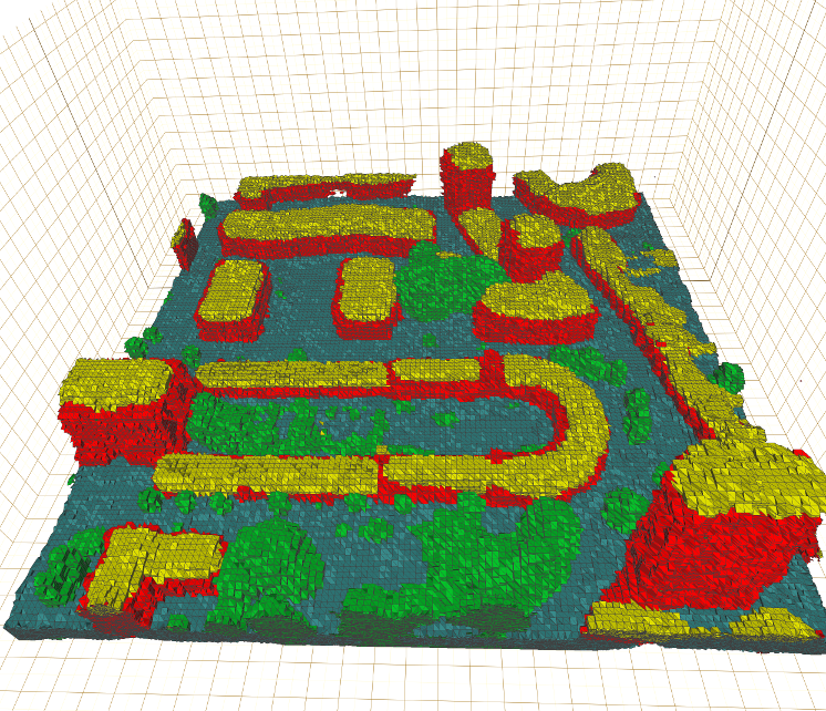
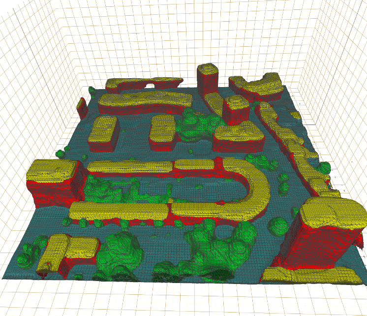
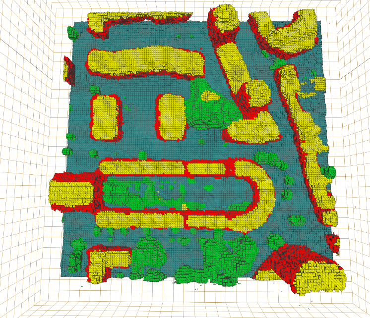
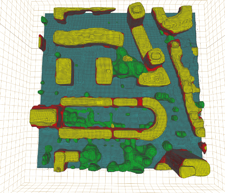
Fig. 16 shows a quantitative evaluation of the Raviart-Thomas basis, equal to the one of the Lagrange basis presented in the main paper. As before, the colors encode building (red), ground (gray), vegetation (green), roof (yellow) and clutter (blue). We summarise the outcomes in Tab. 2. The differences between the Lagrange basis and octree are vanishingly small, on the other hand we notice a bigger gap between the Raviart-Thomas basis and octree. We also present a qualitative comparison of the two bases in Fig. 17. The differences are immediately apparent, which confirms the numbers given in Tab. 2. Raviart-Thomas labels entire simplices, so the reconstruction consists of piecewise constant elements. On the contrary, the Lagrangian basis has the advantage that the labeling functions are linear and can be interpreted as (signed) distance functions, such that a smooth iso-surface can be extracted, here done with marching tetrahedra. Despite the piecewise constant reconstruction, the RT basis measures metric quantities – in contrast to, for instance, Markov random fields, where pairwise distances between the simplices would have to be designed explicitly to achieve similar effects.

Data set	Error measure	Tetra P1	Tetra RT	Octree	MB
Scene 1	Overall acc. [%]	84.0	81.9	83.9	82.5
	Average acc. [%]	81.1	79.1	80.6	81.4

Table 2: Quantitative comparison of our two proposed FEM methods with octree model [Blaha et al.(2016)Blaha, Vogel, Richard, Wegner, Pock, and Schindler] and MultiBoost input data [Benbouzid et al.(2012)Benbouzid, Busa-Fekete, Casagrande, Collin, and Kégl].

Figure 17: Reconstruction with Raviart-Thomas (left) and with the Lagrange basis (right). We deliberately select a low resolution, choose flat shading and plot mesh edges, to accentuate the differences. Please refer to the text for details.

References

- [Bao et al.(2013)Bao, Chandraker, Lin, and Savarese] Yingze Bao, Manmohan Chandraker, Yuanqing Lin, and Silvio Savarese. Dense object reconstruction using semantic priors. In CVPR, 2013.
- [Bartels(2012)] Sören Bartels. Total variation minimization with finite elements: Convergence and iterative solution. SIAM, 50(3), 2012.
- [Benbouzid et al.(2012)Benbouzid, Busa-Fekete, Casagrande, Collin, and Kégl] D. Benbouzid, R. Busa-Fekete, N. Casagrande, F-D. Collin, and B. Kégl. MULTIBOOST: a multi-purpose boosting package. JMLR, 2012.
- [Blaha et al.(2016)Blaha, Vogel, Richard, Wegner, Pock, and Schindler] Maros Blaha, Christoph Vogel, Audrey Richard, Jan Dirk Wegner, Thomas Pock, and Konrad Schindler. Large-scale semantic 3d reconstruction: An adaptive multi-resolution model for multi-class volumetric labeling. In CVPR, 2016.
- [Boyle and Dykstra(1986)] J. P. Boyle and R. L. Dykstra. A method for finding projections onto the intersection of convex sets in Hilbert spaces. Lecture Notes in Statistics, 1986.
- [Bradski(2000)] G. Bradski. The OpenCV Library. Dr. Dobb’s Journal of Software Tools, 2000.
- [Bretin and Masnou(2017)] Elie Bretin and Simon Masnou. A new phase field model for inhomogeneous minimal partitions, and applications to droplets dynamics, 2017.
- [Brezzi and Fortin(1991)] Franco Brezzi and Michel Fortin. Mixed and Hybrid Finite Element Methods. Springer-Verlag New York, 1991.
- [Chambolle and Pock(2011)] Antonin Chambolle and Thomas Pock. A first-order primal-dual algorithm for convex problems with applications to imaging. JMIV, 40(1), 2011.
- [Chambolle et al.(2012)Chambolle, Cremers, and Pock] Antonin Chambolle, Daniel Cremers, and Thomas Pock. A convex approach to minimal partitions. SIAM, 5(4), 2012.
- [Courant(1943)] R. Courant. Variational methods for the solution of problems of equilibrium and vibrations. Bull. Amer. Math. Soc., 49(1), 01 1943.
- [Cremers and Kolev(2011)] D. Cremers and K. Kolev. Multiview stereo and silhouette consistency via convex functionals over convex domains. PAMI, 33(6), 2011.
- [Cremers et al.(2011)Cremers, Pock, Kolev, and Chambolle] D. Cremers, T. Pock, K. Kolev, and A. Chambolle. Convex Relaxation Techniques for Segmentation, Stereo and Multiview Reconstruction. In Advances in Markov Random Fields for Vision and Image Processing. MIT Press, 2011.
- [Curless and Levoy(1996)] Brian Curless and Marc Levoy. A volumetric method for building complex models from range images. SIGGRAPH, 1996.
- [Durán(2008)] Ricardo G. Durán. Mixed Finite Element Methods. Springer Berlin Heidelberg, 2008.
- [Furukawa and Ponce(2010)] Yasutaka Furukawa and Jean Ponce. Accurate, dense, and robust multi-view stereopsis. PAMI, 2010.
- [Grinspun et al.(2002)Grinspun, Krysl, and Schröder] Eitan Grinspun, Petr Krysl, and Peter Schröder. CHARMS: A Simple Framework for Adaptive Simulation. SIGGRAPH, 2002.
- [Häne et al.(2013)Häne, Zach, Cohen, Angst, and Pollefeys] Christian Häne, Christopher Zach, Andrea Cohen, Roland Angst, and Marc Pollefeys. Joint 3d scene reconstruction and class segmentation. In CVPR, 2013.
- [Hirschmüller(2008)] Heiko Hirschmüller. Stereo processing by semiglobal matching and mutual information. PAMI, 2008.
- [Jancosek and Pajdla(2011)] M. Jancosek and T. Pajdla. Multi-view reconstruction preserving weakly-supported surfaces. In CVPR, 2011.
- [Kazhdan et al.(2006)Kazhdan, Bolitho, and Hoppe] Michael Kazhdan, Matthew Bolitho, and Hugues Hoppe. Poisson surface reconstruction. In EUROGRAPHICS, 2006.
- [Kolev et al.(2012)Kolev, Brox, and Cremers] K. Kolev, T. Brox, and D. Cremers. Fast joint estimation of silhouettes and dense 3D geometry from multiple images. PAMI, 2012.
- [Kostrikov et al.(2014)Kostrikov, Horbert, and Leibe] Ilya Kostrikov, Esther Horbert, and Bastian Leibe. Probabilistic labeling cost for high-accuracy multi-view reconstruction. In CVPR, 2014.
- [Kundu et al.(2014)Kundu, Li, Dellaert, Li, and Rehg] Abhijit Kundu, Yin Li, Frank Dellaert, Fuxin Li, and James M. Rehg. Joint semantic segmentation and 3d reconstruction from monocular video. In ECCV, 2014.
- [Labatut et al.(2007)Labatut, Pons, and Keriven] Patrick Labatut, Jean-Philippe Pons, and Renaud Keriven. Efficient Multi-View Reconstruction of Large-Scale Scenes using Interest Points, Delaunay Triangulation and Graph Cuts. In ICCV, 2007.
- [Ladický et al.(2010)Ladický, Sturgess, Russell, Sengupta, Bastanlar, Clocksin, and Torr] Ľubor Ladický, Paul Sturgess, Christopher Russell, Sunando Sengupta, Yalin Bastanlar, William Clocksin, and Philip Torr. Joint optimisation for object class segmentation and dense stereo reconstruction. In BMVC, 2010.
- [Larson and Bengzon(2013)] Mats G. Larson and Fredrik Bengzon. The Finite Element Method: Theory, Implementation, and Applications. Springer Publishing Company, Incorporated, 2013.
- [Lellmann and Schnörr(2011)] Jan Lellmann and Christoph Schnörr. Continuous multiclass labeling approaches and algorithms. SIIMS, 4(4), 2011.
- [Liu and Cooper(2010)] Shubao Liu and David B. Cooper. Ray Markov random fields for image-based 3d modeling: Model and efficient inference. In CVPR, 2010.
- [Lorensen and Cline(1987)] William E. Lorensen and Harvey E. Cline. Marching cubes: A high resolution 3d surface construction algorithm. In SIGGRAPH, 1987.
- [Maggi(2012)] F. Maggi. Sets of Finite Perimeter and Geometric Variational Problems: An Introduction to Geometric Measure Theory. Cambridge Studies in Advanced Mathematics. Cambridge University Press, 2012.
- [Newcombe et al.(2011)Newcombe, Izadi, Hilliges, Molyneaux, Kim, Davison, Kohli, Shotton, Hodges, and Fitzgibbon] Richard A. Newcombe, Shahram Izadi, Otmar Hilliges, David Molyneaux, David Kim, Andrew J. Davison, Pushmeet Kohli, Jamie Shotton, Steve Hodges, and Andrew Fitzgibbon. Kinectfusion: Real-time dense surface mapping and tracking. In ISMAR, Washington, DC, USA, 2011.
- [Nießner et al.(2013)Nießner, Zollhöfer, Izadi, and Stamminger] Matthias Nießner, Michael Zollhöfer, Shahram Izadi, and Marc Stamminger. Real-time 3d reconstruction at scale using voxel hashing. ACM Trans. Graph., 32(6), November 2013.
- [Nieuwenhuis et al.(2013)Nieuwenhuis, Töppe, and Cremers] Claudia Nieuwenhuis, Eno Töppe, and Daniel Cremers. A survey and comparison of discrete and continuous multi-label optimization approaches for the potts model. IJCV, 104(3), 2013.
- [Pock and Chambolle(2011)] Thomas Pock and Antonin Chambolle. Diagonal preconditioning for first order primal-dual algorithms in convex optimization. In ICCV, 2011.
- [Pock et al.(2010)Pock, Cremers, Bischof, and Chambolle] Thomas Pock, Daniel Cremers, Horst Bischof, and Antonin Chambolle. Global solutions of variational models with convex regularization. SIIMS, 3(4), 2010.
- [Reddy(2005)] J. Reddy. An Introduction to the Finite Element Method. McGraw-Hill Education, 2005.
- [Ritz(1909)] Walter Ritz. Über eine neue methode zur lösung gewisser variationsprobleme der mathematischen physik. Journal für die reine und angewandte Mathematik, 1909.
- [Savinov et al.(2015)Savinov, Ladický, Häne, and Pollefeys] Nikolay Savinov, Ľubor Ladický, Christian Häne, and Marc Pollefeys. Discrete optimization of ray potentials for semantic 3d reconstruction. In CVPR, 2015.
- [Steinbruecker et al.(2014)Steinbruecker, Sturm, and Cremers] F. Steinbruecker, J. Sturm, and D. Cremers. Volumetric 3d mapping in real-time on a cpu. In ICRA, 2014.
- [Strekalovskiy and Cremers(2011)] E. Strekalovskiy and D. Cremers. Generalized ordering constraints for multilabel optimization. In ICCV, 2011.
- [Treece(1999)] G. Treece. Regularised marching tetrahedra: improved iso-surface extraction. Computers & Graphics, 23(4), August 1999. ISSN 00978493.
- [Ulusoy et al.(2016)Ulusoy, Black, and Geiger] Ali Osman Ulusoy, Michael J. Black, and Andreas Geiger. Patches, planes and probabilities: A non-local prior for volumetric 3D reconstruction. In CVPR, 2016.
- [Ulusoy et al.(2017)Ulusoy, Black, and Geiger] Ali Osman Ulusoy, Michael J. Black, and Andreas Geiger. Semantic multi-view stereo: Jointly estimating objects and voxels. In CVPR, 2017.
- [Vineet et al.(2015)Vineet, Miksik, Lidegaard, Nießner, Golodetz, Prisacariu, Kähler, Murray, Izadi, Perez, and Torr] Vibhav Vineet, Ondrej Miksik, Morten Lidegaard, Matthias Nießner, Stuart Golodetz, Victor A. Prisacariu, Olaf Kähler, David W. Murray, Shahram Izadi, Patrick Perez, and Philip H. S. Torr. Incremental dense semantic stereo fusion for large-scale semantic scene reconstruction. In ICRA, 2015.
- [Vogiatzis et al.(2007)Vogiatzis, Esteban, Torr, and Cipolla] George Vogiatzis, Carlos Hernández Esteban, Philip H. S. Torr, and Roberto Cipolla. Multiview stereo via volumetric graph-cuts and occlusion robust photo-consistency. PAMI, 29(12), 2007.
- [Vu et al.(2012)Vu, Labatut, Pons, and Keriven] H. H. Vu, P. Labatut, J. P. Pons, and R. Keriven. High accuracy and visibility-consistent dense multiview stereo. PAMI, 34(5), May 2012.
- [Wang and Carreira-Perpiñán(2013)] Weiran Wang and Miguel Á. Carreira-Perpiñán. Projection onto the probability simplex: An efficient algorithm with a simple proof, and an application. CoRR, abs/1309.1541, 2013.
- [Weber et al.(2004)Weber, Blake, and Cipolla] Martin Weber, Andrew Blake, and Roberto Cipolla. Sparse finite elements for geodesic contours with level-sets. In Tomás Pajdla and Jiří Matas, editors, ECCV, 2004.
- [Wu(2011)] Changchang Wu. VisualSFM: A visual structure from motion system, 2011.
- [Zach et al.(2007)Zach, Pock, and Bischof] C. Zach, T. Pock, and H. Bischof. A globally optimal algorithm for robust TV-L1 range image integration. In ICCV, 2007.
- [Zach(2008)] Christopher Zach. Fast and high quality fusion of depth maps. 3DV, 2008.
- [Zach et al.(2014)Zach, Häne, and Pollefeys] Christopher Zach, Christian Häne, and Marc Pollefeys. What is optimized in convex relaxations for multilabel problems: Connecting discrete and continuously inspired MAP inference. PAMI, 2014.