Maximum likelihood estimation of the Latent Class Model through model boundary decomposition

Abstract.

The Expectation-Maximization (EM) algorithm is routinely used for maximum likelihood estimation in latent class analysis. However, the EM algorithm comes with no global guarantees of reaching the global optimum. We study the geometry of the latent class model in order to understand the behavior of the maximum likelihood estimator. In particular, we characterize the boundary stratification of the binary latent class model with a binary hidden variable. For small models, such as for three binary observed variables, we show that this stratification allows exact computation of the maximum likelihood estimator. In this case we use simulations to study the maximum likelihood estimation attraction basins of the various strata and performance of the EM algorithm. Our theoretical study is complemented with a careful analysis of the EM fixed point ideal which provides an alternative method of studying the boundary stratification and maximizing the likelihood function. In particular, we compute the minimal primes of this ideal in the case of a binary latent class model with a binary or ternary hidden random variable.

1. Introduction

Latent class models are popular models used in social sciences and machine learning. They were introduced in the 1950s by Paul Lazarsfeld [24] and were used to find groups in a population based on a hidden attribute (see also [25]). The model obtained its modern probabilistic formulation in the 1970s (e.g.  [17]); we refer to [12] for a more detailed literature review. More recently, latent class models have also become widely used in machine learning, where they are called naive Bayes models. They are a popular method of text categorization, and are also used in other classification schemes [5, Section 8.2.2].

The latent class model is an instance of a model with incomplete data. Maximum likelihood estimation in such models may be challenging, and is typically done using the EM algorithm [9]. Stephen Fienberg in his discussion [11] of the paper introducing the EM algorithm shed some light on its potential problems—his comments are relevant to the latent class model. Referring to [18] Fienberg noted two main problems: (a) even for cases where the log-likelihood for the problem with complete data is concave, the log-likelihood for the incomplete problem need not be concave, and (b) the likelihood equations may not have a solution in the interior of the parameter space. He then wrote:

In the first case multiple solutions of the likelihood equations can exist, not simply a ridge of solutions corresponding to a lack of identification of parameters, and in the second case the solutions of the likelihood equations occur on the boundary of the parameter space,[…].

The latent class model can be formulated as a graphical model with an unobserved variable defined by a star graph like in Figure 1. Given that the variable for the internal vertex was observed, the underlying model becomes a simple instance of an exponential family and, consequently, admits a concave log-likelihood function with a closed formula for the maximizer. However, the marginal likelihood will typically have many critical points, and the maxima may lie on the boundary of the model. In practice, to avoid the boundary problem, Bayesian methods need to be employed to push the solutions away from the boundary by using appropriate priors [14].

Figure 1. The star graph model with $5$ leaves. The internal vertex represents an unobserved random variable.

1.1. Outline of Results

Our aim is to study the boundary problem for the latent class model from the perspective of maximum likelihood estimation. We will use the link between latent class models and nonnegative tensor rank. For instance, the latent class model with three binary observed variables and one binary hidden variable is the model of normalized nonnegative $2\times 2\times 2$ tensors of nonnegative rank ($\text{rank}_{+}$) at most two. We will rely on recent work in algebraic statistics on the description of the (algebraic) boundary of tensors of nonnegative rank two [2]. Our Theorem 9 gives a complete characterization of the boundary strata of binary latent class models with a binary hidden variable.

The geometry of these models allows us to identify boundary strata for which the maximum likelihood problem is easy, such as certain codimension two strata; see Section 4.1. In Section 4.2, we showcase the use of Theorem 9 for the maximum likelihood estimation in the $2\times 2\times 2$ case of $\text{rank}_{+}\leq 2$ by solving the problem exactly: we provide a formula for the maximizer of the likelihood function over the algebraic set defining each boundary strata. Together with recent work in [29], this is the first non-trivial example of the exact solution provided for a latent class model, which typically is fitted using the EM algorithm. The geometry used for this exact solution also provides insight into the maximum likelihood estimation in this model class, validating some of the concerns of Fienberg. We report the results of our simulations which show that the overwhelming majority of data has a maximum likelihood estimator on the boundary of the model (where some model parameters are zero). Indeed, under certain scenarios, even if the true underlying distribution lies in the interior of the model, the maximum likelihood estimator may be found on the boundary with high probability. We also examine briefly the model of $3\times 3\times 2$ tensors of nonnegative rank $3$. Our simulations indicate that this model occupies a tiny portion (approximately $.019\%$) of the probability simplex.

In Section 5, we study the algebraic description of the fixed points of the EM algorithm inspired by [22]. In particular, we compute the irreducible components of the EM fixed point ideal for the $2\times 2\times 2$ tensors of $\text{rank}_{+}\leq 2$ and of $\text{rank}_{+}\leq 3$. In the first case, we demonstrate that we can recover the formulas in Section 4.2 from certain components of the EM fixed point ideal via elimination. In the second case, the irreducible decomposition we compute validates the results in [29] on the boundary decomposition of this model.

2. Definitions and Background

If $X$ is a random variable with values in $\{1,\ldots,k\}$, then its distribution is a point $(p_{1},\ldots,p_{k})$ in the probability simplex

$$\Delta_{k-1}\;\;=\;\;\{(x_{1},\ldots,x_{k})\in\mathbbm{R}^{k}\,:\,x_{1}+\ldots+x_{k}=1,\,\,\,x_{1},\ldots,x_{k}\geq 0\}.$$

The vector $X=(X_{1},\ldots,X_{n})$ is a binary random vector if $X_{i}\in\{1,2\}$ for each $1\leq i\leq n$. A binary tensor $P=(p_{i_{1}\cdots i_{n}})$, where $i_{j}\in\{1,2\}$, is a $2\times 2\times\cdots\times 2$ table of real numbers in ${\mathbb{R}}^{2\times\cdots\times 2}={\mathbb{R}}^{2^{n}}$. A tensor is nonnegative if it has only nonnegative entries. Every probability distribution for a binary vector $X=(X_{1},\ldots,X_{n})$ is a nonnegative binary tensor in the probability simplex $\Delta_{2^{n}-1}$:

$$p_{i_{1}i_{2}\cdots i_{n}}\;=\;{\rm Prob}(\{X_{1}=i_{1},X_{2}=i_{2},\ldots,X_{n}=i_{n}\}).$$

The binary latent class model ${\mathcal{M}}_{n,r}$ is a statistical model for a vector of $n$ binary random variables $X=(X_{1},\ldots,X_{n})$. It contains all distributions such that $X_{1},X_{2},\ldots,X_{n}$ are independent given an unobserved random variable with $r\geq 1$ states. The model is parameterized by the distribution $\lambda=(\lambda_{1},\lambda_{2},\ldots,\lambda_{r})\in\Delta_{r-1}$ of the unobserved variable and the conditional distributions of each $X_{i}$ given the unobserved variable, which we write in form of a stochastic matrix

$$A^{(i)}\,=\,\left(\begin{array}[]{cc}a_{11}^{(i)}&a_{12}^{(i)}\\[8.5359pt] \vdots&\vdots\\[8.5359pt] a_{r1}^{(i)}&a_{r2}^{(i)}\end{array}\right),\;\;\;\;i=1,\ldots,n,$$

where $a_{kl}^{(i)}\geq 0$ and $a_{j1}^{(i)}+a_{j2}^{(i)}=1$ for each $j=1,\ldots,r$. Letting $C_{n}$ denote the $n$-dimensional cube $\Delta_{1}^{n}$, then the parameter space of ${\mathcal{M}}_{n,r}$ is $\Theta:=\Delta_{r-1}\times(C_{n})^{r}$ with elements

$${\theta\;\;=\;\;(\lambda_{1},\ldots,\lambda_{r},\;\;a_{11}^{(1)},a_{12}^{(1)},\ldots,a_{r1}^{(1)},a_{r2}^{(1)},\;\;\ldots,\;\;a_{11}^{(n)},a_{12}^{(n)},\ldots,a_{r1}^{(n)},a_{r2}^{(n)}).}$$

To be succinct, a choice of parameters $\theta$ is also denoted by $\theta=(\boldsymbol{\lambda},A^{(1)},A^{(2)},\ldots,A^{(n)})$. The parameterization $\phi_{n,r}:\>\Theta\to\Delta_{2^{n}-1}$ of ${\mathcal{M}}_{n,r}$ is given by

(1) $$\phi_{n,r}\,:\;\;\;\;\,\theta\;\;\;\;\;\mapsto\;\;\;\;\;p_{j_{1}j_{2}\cdots j_{n}}(\theta)\;\;=\;\;\lambda_{1}a_{1j_{1}}^{(1)}a_{1j_{2}}^{(2)}\cdots a_{1j_{n}}^{(n)}+\cdots+\lambda_{r}a_{rj_{1}}^{(1)}a_{rj_{2}}^{(2)}\cdots a_{rj_{n}}^{(n)}.$$

This parameterization shows that the distributions in ${\mathcal{M}}_{n,r}$ admit a decomposition into $r$ summands, which can be phrased in terms of tensor decompositions. A binary tensor $P$ has rank one if it is an outer product of $n$ vectors in ${\mathbb{R}}^{2}$; that is, there exist $u_{1},\ldots,u_{n}\in{\mathbb{R}}^{2}$ such that $p_{i_{1}i_{2}\cdots i_{n}}=u_{1i_{1}}u_{2i_{2}}\cdots u_{ni_{n}}$. A tensor has nonnegative rank ($\text{rank}_{+}$) at most $r$ if it can be written as a sum of $r$ nonnegative tensors of rank one. Equivalently, a binary tensor with $\text{rank}_{+}\leq r$ is a point in the image of a map $\psi_{n,r}:\>({\mathbb{R}}^{2}_{\geq 0})^{nr}\longrightarrow{\mathbb{R}}^{2^{n}}$ defined as

$$\psi_{n,r}\,:\;\;\,\prod_{i=1}^{n}\prod_{j=1}^{r}(u_{j1}^{(i)},u_{j2}^{(i)})\;\;\;\mapsto\;\;\;p_{i_{1}i_{2}\cdots i_{n}}\;=\;\sum_{j=1}^{r}u_{ji_{1}}^{(1)}u_{ji_{2}}^{(2)}\cdots u_{ji_{n}}^{(n)}.$$

For more on the connection between tensor rank, nonnegative tensor rank, and several of the latent class models under consideration here, see, for example, [1, 8] or for a connection to phylogenetic models [3]. Here we simply formulate the following result.

Proposition 1.

The set of binary tensors with $\text{rank}_{+}\leq r$ is the cone over the binary latent class model ${\mathcal{M}}_{n,r}$.

In this paper we focus primarily on models with two latent classes, $r=2$, and write ${\mathcal{M}}_{n}:={\mathcal{M}}_{n,2}$ and $\phi_{n}:=\phi_{n,2}$. This case in some ways is ‘easy’ since both the algebraic boundary (Proposition 5) and the singular set of the parameterization map (Proposition 6) are well understood. When considering questions of higher nonnegative rank, we have no such tools at our disposal. Binary tensors of $\text{rank}_{+}\leq 2$ were studied in [2], where the following theorem gives a description of $\mathcal{M}_{n}$ as a semi-algebraic set.

Theorem 2.

[2, cf. Theorem 1.1] A binary tensor $P=(p_{i_{1}i_{2}\cdots i_{n}})$ has nonnegative rank at most two if and only if $P$ has flattening rank at most two and $P$ is supermodular.

A matrix flattening of the binary tensor $P$ is a $2^{|\Gamma|}\times 2^{n-|\Gamma|}$ matrix where $\Gamma\subset\{1,\ldots,n\}$ with $1\leq|\Gamma|\leq n-1$. The flattening rank is the maximal rank of any of these matrices. This rank condition provides the equations for the semi-algebraic description since the rank of a matrix is at most two if and only if all $3$-minors of that matrix vanish. Now, we briefly also explain the supermodularity. Let $\pi=(\pi_{1},\ldots,\pi_{n})$ be an $n$-tuple of permutations $\pi_{j}\in S_{2}$. We say $P$ is $\pi$-supermodular if

(2) $$p_{i_{1}i_{2}\cdots i_{n}}\,p_{j_{1}j_{2}\cdots j_{n}}\;\;\leq\;\;p_{k_{1}k_{2}\cdots k_{n}}\,p_{\ell_{1}\ell_{2}\cdots\ell_{n}}$$

holds when $\{i_{s},j_{s}\}=\{k_{s},\ell_{s}\}$ and $\pi_{s}(k_{s})\leq\pi_{s}(\ell_{s})$ for $s=1,\ldots,n$. The tensor $P$ is supermodular if it is $\pi$-supermodular for some $\pi$.

Corollary 3.

The semi-algebraic description of the binary latent class model is given by Theorem 2 together with the extra constraint that $\sum_{i_{1},\ldots,i_{n}}p_{i_{1}\cdots i_{n}}=1$.

We close this section with a result that simplifies some arguments regarding the boundary stratification of ${\mathcal{M}}_{n}$.

Lemma 4.

Let ${\mathcal{M}}_{n,r}$ be the latent class model for the random vector $X=(X_{1},\ldots,X_{n})$, and let $B\subset\{1,\ldots,n\}$ with $|B|=m$. Then the induced marginal model for $X_{B}=(X_{i}\,:\,i\in B)$ is ${\mathcal{M}}_{m,r}$. In particular, if $P$ is a tensor in ${\mathcal{M}}_{n,r}$ given by parameters $(\lambda_{1},\ldots,\lambda_{r}$, $A^{(1)},\ldots,A^{(n)})$, then the corresponding marginal distribution $P_{B}$ is given by parameters $\lambda_{1},\ldots,\lambda_{r}$, and $A^{(i)}$ for $i\in B$.

Proof.

The marginal distribution $P_{B}$ is obtained from $P=(p_{j_{1}\ldots j_{n}})$ by summing over all indices $j_{k}$ with $k\notin B$. When we compute the sum using the parameterization (1) the result follows because $a_{i1}^{(k)}+a_{i2}^{(k)}=1$ for all $i=1,\ldots,r$. ∎

3. Boundary Stratification of ${\mathcal{M}}_{n}$

The semi-algebraic description of ${\mathcal{M}}_{n}$ can also be used to understand the topological boundary of this set. When $n=1,2$, ${\mathcal{M}}_{n}$ is well-understood: ${\mathcal{M}}_{1}=\Delta_{1}$ and ${\mathcal{M}}_{2}=\Delta_{3}$ respectively; see, e.g., [16, Corollary 2.2]. Thus we focus on the case of three or more observed variables, and assume that $n\geq 3$ throughout. We begin our analysis with the following proposition.

Proposition 5.

The dimension of the model ${\mathcal{M}}_{n}$ is $2n+1$. The boundary of this semi-algebraic set is defined by $2n$ irreducible components. Each component is the image of the set in the domain of $\phi_{n}$ given by $a_{1j}^{(i)}=0$ for $i=1,\ldots,n$ and $j=1,2$.

Proof.

The dimension of ${\mathcal{M}}_{n}$ is the number of independent parameters in the domain of $\phi_{n}$. This follows because this model is generically identifiable, which is classically well known; see, e.g [26]. The statement about the boundary is Theorem 1.2 in [2], and the statement about each component is found in the proof of the same result. ∎

Observe that these components are also defined by $a_{2j}^{(i)}=0$, but one can interchange the rows of the matrices $A^{(i)}$ and the entries of $\lambda$, and get the same points on the boundary. This corresponds to ‘label swapping’ on the latent variable. Each component is the collection of tensors where one slice has rank one. By a slice of a tensor $P=(p_{i_{1}\cdots i_{n}})$, we mean a subtensor obtained by fixing one index $i_{k}$. We note that for general tensors with nonnegative rank bigger than two, the boundary of the corresponding model ${\mathcal{M}}$ is not well understood. For instance, points on the boundary of the parameter space defined by setting one parameter equal to zero no longer map to the boundary of the model ${\mathcal{M}}$; see Example 5.2 in [2]. A recent development is [29] where the boundary of ${\mathcal{M}}_{3,3}$ has been described.

In this paper, we consider also lower dimensional pieces of the boundary of ${\mathcal{M}}_{n}$. Our motivation is to perform maximum likelihood estimation over such models efficiently. Proposition 5 implies that various intersections of the $2n$ irreducible codimension one components define lower dimensional boundary pieces. We call a set of boundary points of dimension $k$ obtained as such an intersection a $k$-dimensional stratum. We will identify and describe the boundary strata that are relevant for maximum likelihood estimation. The relevant boundary strata are those which are not degenerate.

Definition 1.

The degenerate part of $\Delta_{2^{n}-1}$ is the set of tensors $P=(p_{i_{1}\cdots i_{n}})$ where for fixed $1\leq j<k\leq n$ and a choice $i_{j}=s$ and $i_{k}=t$ with $s,t\in\{1,2\}$ the entries $p_{i_{1}\cdots s\cdots t\cdots i_{n}}=0$ for all $i_{u}$, $u\neq j,k$.

Another way of detecting that a binary tensor $P$ is degenerate is to look at the marginal table $P_{\{j,k\}}$. If any of the entries of this $2\times 2$ table is zero for any $j,k$, then $P$ is degenerate. For instance, if

$$P_{\{j,k\}}=\left(\begin{array}[]{cc}p_{11}&p_{12}\\ p_{21}&p_{22}\end{array}\right)\,=\,\left(\begin{array}[]{cc}\alpha&0\\ \beta&\gamma\end{array}\right)$$

with $\alpha,\beta,\gamma>0$, then knowing that $X_{j}=1$ implies that $X_{k}=1$. By restricting to nondegenerate tensors, we avoid this kind of probabilistically degenerate situation. We could have formulated our main theorem only for the interior of the probability simplex, since from a mathematical point of view, extending it to some parts of the boundary seems like an incremental gain. From the statistical point of view, however, this gain is quite dramatic as it allows us to understand the maximum likelihood estimator even when data tables contain zeros (as long as two-way marginal tables have no zeros). This is especially important for validating the simulations in Section 4, when the sample sizes are relatively small.

3.1. Singular locus of the parametrization map

To state and prove our main result, we need an understanding of the singular locus of the parameterization map $\phi_{n}$. Recall that a point of the domain $\Theta$ is a singular point of $\phi_{n}$ if the Jacobian of the map drops rank at this point. To describe this set, we look at various (overlapping) subsets of the parameter space. Specifically, let

1. $\Theta_{\lambda_{1}\lambda_{2}}\subseteq\Theta$ be the subset defined by $\lambda_{1}\lambda_{2}=0$;

2. $\Theta_{ij}\subseteq\Theta$ be the subset where $\text{rank}(A^{(k)})=1$ for all $k\neq i,j$ with $1\leq i\neq j\leq n$; and

3. $\Theta_{j}\subseteq\Theta$ be the subset where $\text{rank}(A^{(k)})=1$ for all $k\neq j$.

Finally, we denote by $\Theta^{1}$ the subset of $\Theta$ where $\text{rank}(A^{(k)})=1$ for all $k$. It is clear that $\Theta_{ij}=\Theta_{ji}$ and $\Theta^{1}\subset\Theta_{k}\subset\Theta_{jk}$ for all $1\leq j\neq k\leq n$.

The probabilistic interpretation of these special loci is simple. The set $\Theta_{\lambda_{1}\lambda_{2}}$ corresponds to the parameters for which the latent variable is degenerate taking always the value $0$, or always the value $1$. The set $\Theta_{ij}$ corresponds to the special situation where all variables $X_{k}$ for $k\neq i,j$ are probabilistically independent of the latent variable. That is, only two observable variables in the system carry some information about the latent one. In the case of $\Theta_{j}$, only $X_{j}$ is allowed to nontrivially depend on the latent variable, and $\Theta^{1}$ corresponds to points where all observed random variables are independent of the latent one. Note that the points in the sets $\Theta_{\lambda_{1}\lambda_{2}}$, $\Theta_{j}$, and $\Theta^{1}$ correspond to the situation where all observed variables are independent of each other.

Remark: For those familiar with tensor decompositions, these subsets of parameters have simple descriptions in terms of the ranks of the matrices $A^{(i)}$. Suppose that $\theta=(\boldsymbol{\lambda},A^{(1)},\ldots,A^{(n)})$, then the $m$-rank of $\theta$ is the $n$-tuple $(\text{rank}(A^{(1)}),\ldots,\text{rank}(A^{(n)}))$. In this setting, we see that, for example, $\Theta_{12}$ corresponds to parameters with $m$-rank $(r_{1},r_{2},1,1,\ldots,1)$ with $r_{1},r_{2}\leq 2$. The subset $\Theta_{1}$ corresponds to parameters with $m$-rank $(r_{1},1,1,\ldots,1)$, and $\Theta^{1}$ to those parameters with $m$-rank $(1,1,\dots,1)$. Indeed, this perspective makes it quite easy to determine both the singular locus of $\phi_{n}$ and the tensor rank of the images of these parameter sets.

Proposition 6.

The singular locus of the parametrization map $\phi_{n}$ is equal to

$$\Theta_{\lambda_{1}\lambda_{2}}\cup\bigcup_{1\leq i\neq j\leq n}\Theta_{ij}.$$

This result is not new, cf. [27, Corollary 7.17] and could also be inferred from Theorems 13 and 14 in [15]. We provide an alternative proof that is based on ideas from [1] and [8].

Proof of Proposition 6.

It is clear that the sets $\Theta_{\lambda_{1}\lambda_{2}}$ and $\Theta^{1}$ map under $\phi_{n}$ to distributions in $\mathcal{M}_{n}$ of nonnegative rank $1$, and thus that the Jacobian drops rank at these points. A simple computation shows that $\phi_{n}$ maps points in $\Theta_{k}$ to tensors of $\text{rank}_{+}=1$, and the Jacobian is rank deficient at these parameter points too. Consider now those parameters $\theta$ with (up to permutation) $m$-rank $(2,2,1,\dots,1)$ and, without loss of generality, $\theta\notin\Theta_{\lambda_{1},\lambda_{2}}$. Let $P_{\theta}=\phi_{n}(\theta)$. We quickly show that $P_{\theta}$ has nonnegative rank 2, and that $\theta$ is a singular point of the parameterization. Since $A^{(3)},\ldots,A^{(n)}$ are singular matrices, let $\mathbf{v}$ be the tensor product of their top rows. Stated in more statistical language, $\mathbf{v}$ is the (vectorized) joint distribution of the independent binary variables $X_{3},\ldots,X_{n}$. Using $A^{(1)},A^{(2)}$ for the matrix parameters of rank $2$, then the joint distribution $P_{\theta}$ is $P_{\theta}=(A^{(1)})^{T}\,\operatorname{diag}([\lambda_{1},\lambda_{2}])\,A^{(2)}\otimes\mathbf{v}$. Since $(A^{(1)})^{T}\,\operatorname{diag}([\lambda_{1},\lambda_{2}])\,A^{(2)}$ is a rank 2 matrix, $P_{\theta}$ is a rank 2 tensor. However, the fiber of $P_{\theta}$ is positive dimensional. This follows because the matrix factorization $(A^{(1)})^{T}\,\operatorname{diag}([\lambda_{1},\lambda_{2}])\,A^{(2)}$ above is not unique. If $\Sigma$ is taken to be any matrix sufficiently close to the identity and with column sums equal to $1$, then $\tilde{A}^{(1)}=\Sigma^{T}A^{(1)}$ is Markov, $\tilde{\boldsymbol{\lambda}}=\Sigma^{-1}\operatorname{diag}([\lambda_{1},\lambda_{2}])A^{(2)}\begin{pmatrix}1\\ 1\end{pmatrix}$ has positive entries, $\tilde{A}^{(2)}=\operatorname{diag}(\tilde{\boldsymbol{\lambda}})^{-1}\Sigma^{-1}\operatorname{diag}([\lambda_{1},\lambda_{2}])A^{(2)}$ is Markov, and $\phi_{n}(\tilde{\boldsymbol{\lambda}},\tilde{A}^{(1)},\tilde{A}^{(2)},A^{(3)},\ldots A^{(n)})$ also equals $P_{\theta}$. It follows that $\theta$ is a singular point of the parameterization $\phi_{n}$.

Finally, consider parameters $\theta$ of $m$-rank $(2,2,2,r_{4},\ldots,r_{n})$ up to permutation, $\theta\notin\Theta_{\lambda_{1}\lambda_{2}}$. Then by Kruskal’s Theorem [20, 21] together with techniques developed in [1] for proving parameter identifiability, $\theta$ is identifiable and the fiber of $P_{\theta}$ is of size $2$. This means that $\theta$ is not a singular point of $\phi_{n}$. ∎

We now state and prove two lemmas used repeatedly in the proof of Theorem 9.

Lemma 7.

$\phi_{n}(\Theta_{ij})$ is an $(n+1)$-dimensional subset of $\Delta_{2^{n}-1}$ isomorphic to $\Delta_{3}\times(\Delta_{1})^{n-2}$.

Proof.

A $2\times 2$ stochastic matrix has rank one if and only if both of its rows are equal. Therefore, points in the image of $\Theta_{ij}$ are of the form

$$p_{k_{1}\cdots k_{n}}\;=\;(\lambda_{1}a_{1k_{i}}^{(i)}a_{1k_{j}}^{(j)}+\lambda_{2}a_{2k_{i}}^{(i)}a_{2k_{j}}^{(j)})\prod_{l\neq i,j}a_{1k_{l}}^{(l)}.$$

It is clear that $\phi_{n}(\Theta_{ij})$ is a subset of $\Delta_{2^{n}-1}$ isomorphic to ${\mathcal{M}}_{2}\times(\Delta_{1})^{n-2}$. The equality follows because ${\mathcal{M}}_{2}=\Delta_{3}$. ∎

Lemma 8.

The parametrization $\phi_{n}$ maps $\Theta_{ij}\cap\{a_{st}^{(k)}=0\}$ for $k\neq i,j$ and $s,t\in\{1,2\}$ to the degenerate part of the boundary of $\Delta_{2^{n}-1}$.

Proof.

Consider the case $a_{11}^{(k)}=0$. Then $a_{12}^{(k)}=1$, and since $A^{(k)}$ has rank one we conclude that $a_{21}^{(k)}=0$ and $a_{22}^{(k)}=1$. This means that the first slice of the image tensor along dimension $k$ is identically zero. Similar reasoning applies for all $a_{st}^{(k)}=0$. ∎

Below we consider the intersection of various subsets of the boundary of $\Theta$ with pieces of the singular locus. Motivated by the last lemma, we denote $\Theta_{ij}\cap\mathrm{int}(\Theta)$ by $\Theta_{ij}^{\circ}$. We also let $\Theta_{j}^{\circ}=\Theta_{j}\cap\mathrm{int}(\Theta)$.

3.2. Main Theorem

We now state our main theorem.

Theorem 9.

For $n\leq k\leq 2n+1$, the $k$-dimensional strata of the nondegenerate part of ${\mathcal{M}}_{n}$ are in bijection with the $k-(n+1)$-dimensional faces of the cube $C_{n}$, except for $k=2n-1$ when $n$ additional strata are present, and for $k=n+1$ when ${n\choose 2}$ additional strata are present. More precisely, the stratification of ${\mathcal{M}}_{n}$ has five types of strata:

1. The interior of ${\mathcal{M}}_{n}$. This strata has dimension $2n+1$ and each point is the image under $\phi_{n}$ of a nonsingular point in the interior of $\Theta$.

2. Non-exceptional strata of dimension $n+1\leq k\leq 2n$. Except for $k=2n-1$, each $k$-dimensional stratum is the image of points in

   $$\left(\bigcap_{s_{i}:i\in I}\{a_{1s_{i}}^{(i)}=0\}\right)\,\,\bigcup\,\,\left(\bigcap_{s_{i}:i\in I}\{a_{2s_{i}}^{(i)}=0\}\right),$$

   where $|I|=2n+1-k$. For $k=2n-1$, a stratum corresponding to a codimension two face of $C_{n}$ is the image of points in

   $$\{a_{1s}^{(i)}=0\}\cap\{a_{1t}^{(j)}=0\}\,\bigcup\,\{a_{2s}^{(i)}=0\}\cap\{a_{2t}^{(j)}=0\}\,\bigcup\,\Theta_{ij}^{\circ},$$

   for $1\leq i<j\leq n$ and $s,t=1,2$.

3. Exceptional strata of dimension $2n-1$. These are $n$ additional strata given as the image of points in

   $$\{a_{11}^{(i)}=0\}\cap\{a_{22}^{(i)}=0\}\bigcup\{a_{12}^{(i)}=0\}\cap\{a_{21}^{(i)}=0\},$$

   for $i=1,\ldots,n$.

4. Exceptional strata of dimension $n+1$. These are ${n\choose 2}$ additional strata given as the image of points in $\Theta_{ij}^{\circ}$ for $1\leq i<j\leq n$.

5. A single $n$-dimensional stratum corresponding to the empty face of $C_{n}$ given by the image of points in $\Theta_{\lambda_{1}\lambda_{2}}$.

Corollary 10.

Let $n\leq k\leq 2n+1$ with $k=2n+1-\ell$. Then the number of nondegenerate $k$-dimensional strata of ${\mathcal{M}}_{n}$ is

$$\left\{\begin{array}[]{ll}\displaystyle{n\choose\ell}2^{\ell}&\qquad\ell\neq 2,n,n+1\\[12.0pt] \displaystyle{n\choose 2}4+n&\qquad\ell=2\\[12.0pt] \displaystyle 2^{n}+{n\choose 2}&\qquad\ell=n\\[12.0pt] 1&\qquad\ell=n+1.\end{array}\right.$$

We prove Theorem 9 at the end of this section, after making a few comments about the stratification. As a general rule, the set of probability distributions contained in a single stratum does not allow a clean and simple interpretation. In a few cases, however, we do observe nice patterns, and we describe these below.

(a) Codimension one strata. The $2n$ codimension one strata have a simple recursive description. For example, if $a^{(1)}_{11}=0$ then $a^{(1)}_{12}=1$, and the slice $(p_{1j_{2}\cdots j_{n}})$ of the tensor $P$ is a binary tensor of rank one. This corresponds to the context specific independence model where $X_{2},\ldots,X_{n}$ are independent conditionally on $\{X_{1}=1\}$. It is described in the probability simplex $\Delta_{2^{n-1}-1}$ by the binomial equations

(3) $$p_{1i_{2}\cdots i_{n}}p_{1j_{2}\cdots j_{n}}-p_{1k_{2}\cdots k_{n}}p_{1l_{2}\cdots l_{n}}\;=\;0\quad\mbox{for }\{i_{s},j_{s}\}=\{k_{s},l_{s}\}\mbox{ and }s=2,\ldots,n.$$

The other slice $(p_{2j_{2}\cdots j_{n}})$, after normalization, is a tensor from the model ${\mathcal{M}}_{n-1}$. Hence, knowing the description of ${\mathcal{M}}_{n-1}$ helps describe the codimension one strata of ${\mathcal{M}}_{n}$.

(b) The exceptional codimension two strata (type (3)). If $A^{(1)}$ is the identity matrix, then the parameterization in (1) specializes to

$$p_{1j_{2}\cdots j_{n}}=\lambda_{1}a_{1j_{2}}^{(2)}\cdots a_{1j_{n}}^{(n)},\qquad p_{2j_{2}\cdots j_{n}}=\lambda_{2}a_{2j_{2}}^{(2)}\cdots a_{2j_{n}}^{(n)}.$$

Since $A^{(2)},\ldots,A^{(n)}$ are arbitrary stochastic matrices, the first stratum of type (3) corresponds to the model where $X_{2},\ldots,X_{n}$ are independent conditionally on $X_{1}$. This is a graphical model given by the graph in Figure 2. This model is fully described in the probability simplex $\Delta_{2^{n}-1}$ by the binomial equations

$$p_{ii_{2}\cdots i_{n}}p_{ij_{2}\cdots j_{n}}-p_{ik_{2}\cdots k_{n}}p_{il_{2}\cdots l_{n}}\;=\;0\quad\mbox{for $i=1,2$, }\{i_{s},j_{s}\}=\{k_{s},l_{s}\}\mbox{ and }s=2,\ldots,n$$

with no additional inequalities. The analysis is analogous for the $n-1$ remaining strata given by one of $A^{(2)},\ldots,A^{(n)}$ being the identity matrix.

(c) The $n$-dimensional stratum (type(5)). This unique stratum is given by all rank one tensors in $\Delta_{2^{n}-1}$. This stratum is defined by the equations

$$p_{i_{1}i_{2}\cdots i_{n}}p_{j_{1}j_{2}\cdots j_{n}}-p_{k_{1}k_{2}\cdots k_{n}}p_{l_{1}l_{2}\cdots l_{n}}\;=\;0\quad\mbox{if }\{i_{s},j_{s}\}=\{k_{s},l_{s}\}\mbox{ for }s=1,\ldots,n$$

and it corresponds to the full independence model.

Figure 2. The graph representing the strata given by $a^{(1)}_{12}=a^{(1)}_{21}=0$.

The strata of ${\mathcal{M}}_{n}$ form a partially ordered set where for two strata $S,S^{\prime}$ we have $S\preceq S^{\prime}$ if the closure of $S$ is contained in the closure of $S^{\prime}$. Such a partially ordered set structure becomes important in Section 4 to provide further insights into the geometry of the maximum likelihood estimation. Suppose that $p^{*}$ is a maximizer of a function $f$ over the (Zariski) closure of a set $S^{\prime}$. If $S$ is another set such that $S\preceq S^{\prime}$ then the value of $f$ in $S$ is bounded above by $f(p^{*})$. In particular, if $p^{*}$ lies in $S^{\prime}$ then to maximize $f$ over ${\mathcal{M}}_{n}$ there is no need to check strata $S$ such that $S\preceq S^{\prime}$.

The interior of ${\mathcal{M}}_{n}$ is the unique maximal element, and the unique strata of type (5) is the unique minimal element. For example, for ${\mathcal{M}}_{3}$ there are six dimension 6 strata, which we label by $\{1,2,3,4,5,6\}$ corresponding to equations

$$(1)\;\;\;p_{111}p_{122}=p_{112}p_{121}\qquad(2)\;\;\;p_{211}p_{222}=p_{212}p_{221}$$

$$(3)\;\;\;p_{111}p_{212}=p_{112}p_{211}\qquad(4)\;\;\;p_{121}p_{222}=p_{122}p_{221}$$

$$(5)\;\;\;p_{111}p_{221}=p_{121}p_{211}\qquad(6)\;\;\;p_{112}p_{222}=p_{122}p_{212}$$

respectively. These six equations are naturally grouped in pairs as indicated by the three rows above. Each of these three pairs defines one of the three special strata of type (3). In general, each special stratum of this kind is obtained as the intersection of codimension one strata which correspond to “opposite” facets of $C_{n}$. For ${\mathcal{M}}_{3}$, each special stratum of type (4) is defined by four equations found in two rows of the six equations above. If one ignores these special strata, the poset is isomorphic to the face poset of the cube $C_{n}$. The Hasse diagram of the poset for ${\mathcal{M}}_{3}$ is given in Figure 3.

Figure 3. The boundary stratification poset of ${\mathcal{M}}_{3}$. The red and blue nodes correspond to strata of type (3) and of type (4), respectively.

We now turn to the proof of Theorem 9. The result will follow from a sequence of lemmas. By Proposition 5 there are exactly $2n$ strata of codimension one, each consisting of tensors where in one slice along a given dimension the subtensor has rank at most one. In other words, each stratum is described by a collection of equations of the form (3) together with the inequalities forcing supermodularity. We denote these strata by $\Gamma_{is}$ where $i=1,\ldots,n$ and $s=1,2$.

We first formulate a lemma that shows that boundary points are mapped to boundary points under the marginalization $P\mapsto P_{B}$ (c.f. Lemma 4).

Lemma 11.

Suppose that $n\geq 4$ and let $B\subset\{1,\ldots,n\}$ with $|B|=m\geq 3$. For $i\in B$, if a point $P$ in ${\mathcal{M}}_{n}$ lies on $\Gamma_{is}$, then $P_{B}$ lies in the corresponding stratum $\Gamma_{is}$ of the marginal model ${\mathcal{M}}_{m}$.

Proof.

If $P$ is the image of $(\lambda_{1},\lambda_{2},A^{(k)}\,:\,k=1,\ldots,n)$, by Lemma 4, $P_{B}$ is the image of $(\lambda_{1},\lambda_{2},A^{(k)}\,:\,k\in B)$. Hence if the slice $s$ in dimension $i$ of $P$ has rank one, so will the slice $s$ in dimension $i$ of $P_{B}$. ∎

Proposition 12.

The preimage of the codimension one stratum $\Gamma_{is}$ under $\phi_{n}$ is

$$\phi_{n}^{-1}(\Gamma_{is})\,=\,\{a_{1s}^{(i)}=0\}\cup\{a_{2s}^{(i)}=0\}\cup\Theta_{\lambda_{1}\lambda_{2}}\cup\bigcup_{k\neq i}\Theta_{ik}^{\circ}.$$

Proof.

We first show that

$$\{a_{1s}^{(i)}=0\}\cup\{a_{2s}^{(i)}=0\}\cup\Theta_{\lambda_{1}\lambda_{2}}\cup\bigcup_{k\neq i}\Theta_{ik}^{\circ}\;\;\subset\;\;\phi_{n}^{-1}(\Gamma_{is}).$$

Clearly $\{a_{1s}^{(i)}=0\}\cup\{a_{2s}^{(i)}=0\}\cup\Theta_{\lambda_{1}\lambda_{2}}$ lies in the preimage. To show that the preimage contains also $\Theta_{ik}^{\circ}$ for each $k\neq i$, note that the image of a point in $\Theta_{ik}^{\circ}$ is given by

$$p_{j_{1}\cdots j_{i}\cdots j_{k}\cdots j_{n}}=(\lambda_{1}a_{1j_{i}}^{(i)}a_{1j_{k}}^{(k)}+\lambda_{2}a_{2j_{i}}^{(i)}a_{2j_{k}}^{(k)})\prod_{l\neq i,k}a_{1j_{l}}^{(l)}.$$

The points on $\Gamma_{is}$ must satisfy $p_{i_{1}\cdots s\cdots i_{n}}p_{j_{1}\cdots s\cdots j_{n}}=p_{\nu_{1}\cdots s\cdots\nu_{n}}p_{\mu_{1}\cdots s\cdots\mu_{n}}$ for $\{i_{t},j_{t}\}=\{\nu_{t},\mu_{t}\}$ where $1\leq t\neq i\leq n$. The above point satisfies such equations since

$$(\lambda_{1}a_{1s}^{(i)}a_{1i_{k}}^{(k)}+\lambda_{2}a_{2s}^{(i)}a_{2i_{k}}^{(k)})(\lambda_{1}a_{1s}^{(i)}a_{1j_{k}}^{(k)}+\lambda_{2}a_{2s}^{(i)}a_{2j_{k}}^{(k)})=$$

$$(\lambda_{1}a_{1s}^{(i)}a_{1\nu_{k}}^{(k)}+\lambda_{2}a_{2s}^{(i)}a_{2\nu_{k}}^{(k)})(\lambda_{1}a_{1s}^{(i)}a_{1\mu_{k}}^{(k)}+\lambda_{2}a_{2s}^{(i)}a_{2\mu_{k}}^{(k)}).$$

Next we show that no other points lie in the preimage. To this end, from now on suppose that $a_{1s}^{(i)}\neq 0$, $a_{2s}^{(i)}\neq 0$, $\lambda_{1}\cdot\lambda_{2}\neq 0$ and the parameters are not in $\bigcup_{k\neq i}\Theta_{ik}^{\circ}$. Hence we can assume that $P\in\Gamma_{is}$ is given by a parameter vector such that for some $j,k\neq i$ the matrices $A^{(j)},A^{(k)}$ have rank $2$. Consider the marginal distribution over $\{i,j,k\}$ and denote its coordinates by $q_{u_{i}u_{j}u_{k}}$, $u_{i},u_{j},u_{k}\in\{1,2\}$. By Lemma 11, it is a point in ${\mathcal{M}}_{3}$ parameterized by $(\lambda_{1},\lambda_{2},A^{(i)},A^{(j)},A^{(k)})$, and it satisfies $q_{s11}q_{s22}=q_{s12}q_{s21}$. A quick computation shows that this is equivalent to

(4) $$\lambda_{1}\lambda_{2}a_{1s}^{(i)}a_{2s}^{(i)}\det(A^{(j)})\det(A^{(k)})\;=\;0.$$

However, by our assumption, this is impossible. ∎

Our strategy to prove Theorem 9 is to intersect preimages of codimension one strata $\Gamma_{is}$. By Proposition 12, this means we must consider intersections of subsets of the boundary of the parameter space $\Theta$ and of various subsets of the singular locus of $\phi_{n}$ in the interior of $\Theta$. When doing this, we disregard two types of intersections. The first type consists of subsets of the parameter space whose points map to the degenerate part of $\Delta_{2^{n}-1}$. Since we are interested in nondegenerate points in the intersections of $\Gamma_{is}$, these kinds of subsets are irrelevant. The second type consists of subsets of the parameter space whose points map to tensors of rank one. The next proposition justifies the irrelevance of these subsets.

Proposition 13.

The intersection of all $\Gamma_{is}$ for $i=1,\ldots,n$ and $s=1,2$ contains all tensors of rank one.

Proof.

Every tensor in $\Delta_{2^{n}-1}$ of rank one is the image of a parameter vector in $\Theta$ where $\lambda_{1}=0$. Such a parameter vector is in $\Theta_{\lambda_{1}\lambda_{2}}$. By Proposition 12, the image of $\Theta_{\lambda_{1}\lambda_{2}}$ under the parametrization map is contained in every $\Gamma_{is}$. ∎

In Corollary 22 we prove that the intersection of all nondegenerate points in $\Gamma_{is}$ for $i=1,\ldots,n$, $s=1,2$ is equal to the set of nondegenerate tensors of rank one. This intersection gives us the unique $n$-dimensional stratum (type (5)). Hence, when intersecting preimages of $\Gamma_{is}$ we ignore parameters mapping to tensors of rank one since their images are in every possible intersection. In summary, when we refer to intersections of $\phi_{n}^{-1}(\Gamma_{is})$ we consider only the relevant part, meaning only those points that do not map to degenerate or rank one tensors. For instance, by Proposition 12 the relevant part of $\phi_{n}^{-1}(\Gamma_{is})$ consists of $\{a_{1s}^{(i)}=0\}\cup\{a_{2s}^{(i)}=0\}\cup\bigcup_{k\neq i}\Theta_{ik}^{\circ}$.

Lemma 14.

The relevant part of $\phi_{n}^{-1}(\Gamma_{is})\cap\phi_{n}^{-1}(\Gamma_{jt})$ where $i\neq j$ is

$$\{a_{1s}^{(i)}=0\}\cap\{a_{1t}^{(j)}=0\}\,\bigcup\,\{a_{2s}^{(i)}=0\}\cap\{a_{2t}^{(j)}=0\}\,\bigcup\,\Theta_{ij}^{\circ}.$$

Proof.

The points in the set $\{a_{1s}^{(i)}=0\}\cap\{a_{2t}^{(j)}=0\}$ map to degenerate tensors since in the marginalization of the image tensor $P_{\{i,j\}}(X_{i}=s,X_{j}=t)=0$. A similar argument shows that $\{a_{2s}^{(i)}=0\}\cap\{a_{1t}^{(j)}=0\}$ is irrelevant. So we just need to compute the intersection of $\cup_{k\neq i}\Theta_{ik}^{\circ}$ and $\cup_{\bar{k}\neq j}\Theta_{j\bar{k}}^{\circ}$. When $k=j$ and $\bar{k}=i$, we get $\Theta_{ij}^{\circ}$. Also, $\Theta_{ij}^{\circ}\cap\Theta_{j\bar{k}}=\Theta_{j}^{\circ}$ when $\bar{k}\neq i$, and $\Theta_{ik}^{\circ}\cap\Theta_{ji}=\Theta_{i}^{\circ}$ when $k\neq j$. Both are irrelevant. For the case $k\neq j$ and $\bar{k}\neq i$, we either get $\Theta^{1}$ if $k\neq\bar{k}$, or $\Theta_{k}^{\circ}$ if $k=\bar{k}$. Again both cases give irrelevant subsets. ∎

Corollary 15.

The nondegenerate intersection of $\Gamma_{is}$ with $\Gamma_{jt}$ where $i\neq j$ is a stratum of dimension $2n-1$. There are ${n\choose 2}4$ such strata.

Proof.

The parametrization map $\phi_{n}$ is generically smooth on $\bigcup_{u=1,2}\{a_{us}^{(i)}=0\}\cap\{a_{ut}^{(j)}=0\}$, and a simple parameter count shows that this set has dimension equal to $2n-1$. Together with Lemma 7 this implies the result. For each $1\leq i<j\leq n$ and each choice of $s,t\in\{1,2\}$ we get such a stratum. Hence, there are ${n\choose 2}4$ of them. ∎

Lemma 16.

The relevant part of $\phi_{n}^{-1}(\Gamma_{i1})\cap\phi_{n}^{-1}(\Gamma_{i2})$ is

$$\{a_{11}^{(i)}=0\}\cap\{a_{22}^{(i)}=0\}\bigcup\{a_{12}^{(i)}=0\}\cap\{a_{21}^{(i)}=0\}\bigcup\cup_{k\neq i}\Theta_{ik}^{\circ}.$$

Proof.

The intersections $\{a_{11}^{(i)}=0\}\cap\{a_{12}^{(i)}=0\}$ and $\{a_{21}^{(i)}=0\}\cap\{a_{22}^{(i)}=0\}$ are empty in the parameter space $\Theta$. ∎

Corollary 17.

The nondegenerate intersection $\Gamma_{i1}\cap\Gamma_{i2}$ is a stratum of dimension $2n-1$. There are $n$ such exceptional strata.

Proof.

The parametrization map $\phi_{n}$ is generically smooth on $\{a_{11}^{(i)}=0\}\cap\{a_{22}^{(i)}=0\}$, and on $\{a_{12}^{(i)}=0\}\cap\{a_{21}^{(i)}=0\}$, and the dimension of this set is $2n-1$. Together with Lemma 7 this gives the first statement. The count is obvious. ∎

Lemma 18.

The relevant part of $\phi_{n}^{-1}(\Gamma_{is})\cap\phi_{n}^{-1}(\Gamma_{jt})\cap\phi_{n}^{-1}(\Gamma_{kv})$ where $i,j,k$ are distinct is

$$\bigcup_{u=1,2}\{a_{us}^{(i)}=0\}\cap\{a_{ut}^{(j)}=0\}\cap\{a_{uv}^{(k)}=0\}.$$

Proof.

We proceed as in the proof Lemma 14. After discarding irrelevant subsets such as $\{a_{1s}^{(i)}=0\}\cap\{a_{1t}^{(j)}=0\}\cap\{a_{2v}^{(k)}=0\}$ (since they map to degenerate tensors) we also see that the desired intersection contains $\Theta_{ij}^{\circ}\cap\Theta_{ik}^{\circ}\cap\Theta_{jk}^{\circ}=\Theta^{1}$. This is also irrelevant. ∎

This result immediately generalizes to higher-order intersections.

Corollary 19.

Let $I\subset\{1,\ldots,n\}$ where $|I|=\ell\geq 3$. Then for each choice of $s_{i}\in\{1,2\}$ for $i\in I$ the nondegenerate intersection $\bigcap_{i\in I}\Gamma_{is_{i}}$ is a stratum of dimension $2n+1-\ell$. There are ${n\choose\ell}2^{\ell}$ such strata.

Proof.

Lemma 18 implies that the relevant part of $\bigcap_{i\in I}\phi_{n}^{-1}(\Gamma_{is_{i}})$ is

$$\bigcup_{u=1,2}\left(\bigcap_{s_{i}:i\in I}\{a_{us_{i}}^{(i)}=0\}\right).$$

Each piece of this union has dimension $2n+1-\ell$, and since $\phi_{n}$ is generically smooth on these sets the intersection $\bigcap_{i\in I}\Gamma_{is_{i}}$ is a stratum of the same dimension. It is easy to count such strata. ∎

Lemma 20.

The relevant part of $\phi_{n}^{-1}(\Gamma_{i1})\cap\phi_{n}^{-1}(\Gamma_{i2})\cap\phi_{n}^{-1}(\Gamma_{j1})$ is $\Theta_{ij}^{\circ}$. Moreover, this is equal to the relevant part of $\phi_{n}^{-1}(\Gamma_{i1})\cap\phi_{n}^{-1}(\Gamma_{i2})\cap\phi_{n}^{-1}(\Gamma_{j1})\cap\phi_{n}^{-1}(\Gamma_{j2})$.

Proof.

We have computed $\phi_{n}^{-1}(\Gamma_{i1})\cap\phi_{n}^{-1}(\Gamma_{i2})$ in Lemma 16. Together with Proposition 12 we conclude that we need to describe the intersection of

$$\{a_{11}^{(i)}=0\}\cap\{a_{22}^{(i)}=0\}\bigcup\{a_{12}^{(i)}=0\}\cap\{a_{21}^{(i)}=0\}\bigcup\cup_{k\neq i}\Theta_{ik}^{\circ}$$

with

$$\{a_{11}^{(j)}=0\}\cup\{a_{21}^{(j)}=0\}\bigcup\cup_{k\neq j}\Theta_{jk}^{\circ}.$$

Up to symmetry, we get the following intersections: (i) $\{a_{12}^{(i)}=0,a_{21}^{(i)}=0,a_{11}^{(j)}=0\}$, (ii) $\Theta^{\circ}_{ij}$. It is therefore enough to show that the first set is irrelevant. Let $P$ be a tensor that is in the image of a point in the set (i). Then in the marginal distribution $P_{\{i,j\}}$ we have $P_{\{i,j\}}(X_{i}=1,X_{j}=1)=0$. Hence $P$ is degenerate. Finally, when we intersect further with $\phi_{n}^{-1}(\Gamma_{j2})=\{a_{12}^{(j)}=0\}\cup\{a_{22}^{(j)}=0\}\cup\bigcup_{k\neq j}\Theta_{jk}^{\circ}$, still the only thing that survives as relevant is $\Theta_{ij}^{\circ}$. ∎

Corollary 21.

For $i\neq j$, the nondegenerate points in the intersection $\Gamma_{i1}\cap\Gamma_{i2}\cap\Gamma_{j1}\cap\Gamma_{j2}$ is a stratum of dimension $n+1$. There are ${n\choose 2}$ such strata.

Proof.

The nondegenerate intersection given in the statement is the image of $\Theta_{ij}^{\circ}$ by Lemma 20. This intersection is not contained in any other $\Gamma_{k1}$ or $\Gamma_{k2}$ for $k\neq i,j$ since by Proposition 12 everything in $\Theta_{ij}^{\circ}\cap\phi_{n}^{-1}(\Gamma_{k1})$ maps to tensors of rank one. Hence, indeed $\Gamma_{i1}\cap\Gamma_{i2}\cap\Gamma_{j1}\cap\Gamma_{j2}$ defines a stratum. Lemma 7 implies that the dimension of this stratum is $n+1$. Clearly, there are ${n\choose 2}$ such strata. ∎

Corollary 22.

The intersection of all nondegenerate points in $\Gamma_{is}$ for $i=1,\ldots,n$, $s=1,2$ is the unique stratum of dimension $n$ consisting of all nondegenerate tensors of rank one.

Proof.

From Proposition 13 the intersection contains the set of tensors of rank one. Corollary 21 implies that $\bigcap_{s=1,2}\left(\Gamma_{is}\cap\Gamma_{js}\cap\Gamma_{ks}\right)$ is contained in the set of tensors of rank one establishing that the intersection of all codimension one strata is a stratum. The dimension of the set of rank one tensors is $n$. ∎

Finally, we prove the main theorem.

Proof of Theorem 9: Proposition 5 implies that the interior of ${\mathcal{M}}_{n}$ has dimension $2n+1$. The above results imply that any parameter vector with $a_{1s}^{(i)}=0$ or $a_{2s}^{(i)}=0$ for $s=1,2$ maps to the algebraic boundary of ${\mathcal{M}}_{n}$. Similarly, any parameter vector in $\Theta_{ij}^{\circ}$ for $1\leq i\neq j\leq n$ as well as a parameter vector in $\Theta_{\lambda_{1}\lambda_{2}}$ is mapped to the boundary of ${\mathcal{M}}_{n}$. The remaining parameter vectors must map to the interior of ${\mathcal{M}}_{n}$, and these points are nonsingular parameter vectors that are in the interior of $\Theta$. We will associate the interior of ${\mathcal{M}}_{n}$ with the interior of the $n$-dimensional cube $C_{n}$.

Also by Proposition 5, $\Gamma_{is}$ for $i=1,\ldots,n$ and $s=1,2$ are precisely the $2n$ boundary strata of dimension $2n$. They are in bijection with the $2n$ facets of $C_{n}$. By Proposition 12, the preimage of each $\Gamma_{is}$ is $\{a_{1s}^{(i)}=0\}\cup\{a_{2s}^{(i)}=0\}\cup\Theta_{\lambda_{1}\lambda_{2}}\cup\bigcup_{k\neq i}\Theta_{ik}^{\circ}$. Lemma 14 proves that $\Gamma_{is}\cap\Gamma_{jt}$ for $i\neq j$ is the image of points in $\{a_{1s}^{(i)}=0\}\cap\{a_{1t}^{(j)}=0\}\,\bigcup\,\{a_{2s}^{(i)}=0\}\cap\{a_{2t}^{(j)}=0\}\,\bigcup\,\Theta_{ij}^{\circ}$. By Corollary 15 this is the non-exceptional strata of dimension $k=2n-1$ and these strata correspond to $(n-2)$-dimensional faces of $C_{n}$ which are obtained as intersections of nonparallel facets of the cube (i.e. $i\neq j$). Lemma 18 and Corollary 19 take care of the non-exceptional strata of dimension $n<k<2n-1$ as the image of $\bigcup_{u=1,2}\left(\bigcap_{s_{i}:i\in I}\{a_{us_{i}}^{(i)}=0\}\right)$. This image is the intersection of $\bigcap_{i\in I}\Gamma_{is_{i}}$ where $|I|=2n+1-k$. They correspond to faces of $C_{n}$ of dimension $k-n-1$. This describes all nondegenerate strata of types (1) and (2) in the statement of the theorem.

The exceptional strata of codimension two ($k=2n-1$), that is of type (3), is described by Lemma 16 and Corollary 17, combined with the proof of Lemma 4.5 in [2]. The statement about the exceptional strata (type (4)) of dimension $k=n+1$ follows from Lemma 20 and Corollary 21. And finally, the proof of Lemma 20 and Corollary 22 provide the description of the unique $n$-dimensional stratum given in type (5). $\Box$

4. Maximum likelihood estimation over ${\mathcal{M}}_{n}$

In this section we present how our understanding of the boundary of ${\mathcal{M}}_{n}$ provides a partial understanding of the maximum likelihood estimation over this model class. For ${\mathcal{M}}_{3}$, maximum likelihood estimators are computed exactly.

Suppose an independent sample of size $N>1$ was observed from a binary distribution. We report the data in a tensor of counts $U=(u_{i_{1}\cdots i_{n}})$ where $u_{i_{1}\cdots i_{n}}$ is the number of times the event $\{X_{1}=i_{1},\ldots,X_{n}=i_{n}\}$ was observed. The sum of all elements in $U$ is equal to $N$. The log-likelihood function $\ell:\,\Theta\longrightarrow{\mathbb{R}}$ is

(5) $$\ell(\theta)\;=\;\sum_{i_{1},\ldots,i_{n}=1}^{2}u_{i_{1}\cdots i_{n}}\log(p_{i_{1}\cdots i_{n}}(\theta)),$$

where $p_{i_{1}\cdots i_{n}}(\theta)$ is as in (1). In this section we are interested in maximizing the log-likelihood function over ${\mathcal{M}}_{n}$ to compute a maximum likelihood estimate (MLE) for the data $U$. We remark that $\ell(\theta)$ is a strictly concave function on the entire $\Delta_{2^{n}-1}$, and if its unique maximizer over the entire probability simplex is not in ${\mathcal{M}}_{n}$, then its maximizer over ${\mathcal{M}}_{n}$, i.e. the MLE, must be on the boundary of ${\mathcal{M}}_{n}$.

In our analysis of boundary strata we restricted attention to nondegenerate tensors in $\Delta_{2^{n}-1}$. The lemma below ensures that by looking at the data $U$ we can detect when the MLE is going to lie in this nondegenerate part, and so, when we can apply Theorem 9. It implies that if the sample proportions tensor $Q=\frac{1}{N}U$ lies outside the degenerate part of $\Delta_{2^{n}-1}$, then the MLE $\hat{P}$ over ${\mathcal{M}}_{n}$ will also be nondegenerate.

Lemma 23.

Let ${\mathcal{M}}$ be a model in $\Delta_{k-1}$ for some $k\geq 1$ and let $Q=\frac{1}{N}U$ be the sample proportions for data $U$. Then if the MLE $\hat{P}$ for $U$ exists, the support of $Q$ is contained in the support of $\hat{P}$.

Proof.

The MLE is the constrained maximizer over ${\mathcal{M}}$ of the log-likelihood

$$\sum_{i=1}^{k}u_{i}\log P_{i}\;=\;\sum_{i\in{\rm supp}(Q)}u_{i}\log P_{i}.$$

It is equal to $-\infty$ at all points $P$ with $P_{i}=0$ for some $i\in{\rm supp}(Q)$. ∎

4.1. General results

In order to solve the optimization problem for the log-likelihood (5), one can compute all critical points of $\ell(\theta)$ over the interior and all boundary strata of ${\mathcal{M}}_{n}$. For many parametrized statistical models the equations defining these critical points are just rational functions in the parameter vector $\theta$. This is the case for the latent class models that we study in this paper. We will call the number of complex critical points of $\ell(\theta)$ over a model for generic data $U$ the maximum likelihood degree (ML-degree) of that model. The ML-degree for general algebraic statistical models were introduced in [7] and [19]. In particular, it was shown that the ML-degree of such a model is a stable number. We will use the ML-degrees of the boundary strata of ${\mathcal{M}}_{n}$ as an indication for the complexity of solving the maximum likelihood estimation problem. For instance, if the ML-degree is $\leq 4$, then one can express the MLE with closed form formulas as a function of $U$. In particular, if the ML-degree is equal to one, then the MLE can be expressed as a rational function of $U$.

In order to solve the constrained optimization problem of maximizing the likelihood function, one can employ the following simple scheme:

• For each stratum $S$ of ${\mathcal{M}}_{n}$ list the critical points of the log-likelihood function constrained to its closure $\overline{S}$.

• Pick the best point from the list of those critical points that lie in ${\mathcal{M}}_{n}$.

Our first observation for this procedure is that we never need to check all the strata to find a global maximum. To see this consider the poset of the boundary stratification as described in the previous section. In our search for the global maximum we start from the maximal element of the poset and move recursively down. If a global maximum over the closure $\overline{S}$ lies in the stratum $S$, there is no need to optimize over any stratum $S^{\prime}\preceq S$. As shown below, for many strata the MLE is guaranteed to lie inside ${\mathcal{M}}_{n}$.

A second observation is that maximizing the log-likelihood over most of the strata is challenging. The defining constraints correspond to complicated context specific independence constraints [6], and there is as yet no general theory on how to optimize over these models exactly. There are, however, several exceptions including the strata considered in Section 3. We begin by introducing notation used below: For the data tensor $U=(u_{i_{1}\cdots i_{n}})$ denote by $U^{(s,t)}=(u^{(s,t)}_{ij})$ the matrix whose $(i,j)$-th entry is the count of the event $\{X_{s}=i,X_{t}=j\}$ and by $U^{(s)}=(u^{(s)}_{i})$ the vector whose entries are the counts of the event $\{X_{s}=i\}$.

(a) Codimension one strata (type (2), $k=2n$). Each tensor on one of these $2n$ strata corresponds to a context specific independence model, such as where $X_{2},\ldots,X_{n}$ are independent conditionally on $\{X_{1}=1\}$. The ML-degree of the corresponding conditional model is one; hence, the MLE is expressed as a rational function of the data:

$$\hat{p}_{1j_{2}\cdots j_{i}\cdots j_{n}}\;\;=\;\;\frac{u_{1j_{2}}^{(12)}u_{1j_{3}}^{(13)}\cdots u_{1j_{n}}^{(1n)}}{N{u_{1}^{(1)}}^{n-2}}.$$

After normalization, the other slice is a tensor from the model ${\mathcal{M}}_{n-1}$. Therefore $\hat{p}_{2j_{2}\cdots j_{i}\cdots j_{n}}$ can be computed by employing any procedure that can be used for ${\mathcal{M}}_{n-1}$. For instance, in the next section we derive a closed form formula for the maximizer on each boundary stratum of ${\mathcal{M}}_{3}$. Hence, in the case of ${\mathcal{M}}_{4}$ all codimension one strata will also have closed form formulas.

(b) The exceptional codimension two strata of type (3). As noted in Section 3, these strata correspond to simple graphical models over graphs like that in Figure 2. The ML-degree of this model is one; hence, the MLE is expressed as a rational function of the data (also see [23, Section 4.4.2]):

$$\hat{p}_{j_{1}j_{2}\cdots j_{i}\cdots j_{n}}\;\;=\;\;\frac{u_{j_{1}j_{2}}^{(12)}u_{j_{1}j_{3}}^{(13)}\cdots u_{j_{1}j_{n}}^{(1n)}}{N{u_{j_{1}}^{(1)}}^{n-2}}.$$

This point is always guaranteed to lie in ${\mathcal{M}}_{n}$ and so we never have to check strata that lie below that in the Hasse diagram defined in the previous section. These are the ${n\choose 2}$ strata of type (4) and the type (5) stratum. Nevertheless, optimizing over these special strata is simple so we describe it next.

(c) The $(n+1)$-dimensional strata of type (4). These strata correspond to graphical models with one edge and $n-2$ disconnected nodes. The ML-degree of this model is one. For example, if $1$ and $2$ are connected by an edge and all other nodes are disconnected, the MLE is

$$\hat{p}_{j_{1}j_{2}j_{3}\cdots j_{n}}\;\;=\;\;\frac{1}{N^{n-1}}u^{(12)}_{j_{1}j_{2}}u^{(3)}_{j_{3}}\cdots u^{(n)}_{j_{n}}.$$

(d) The $n$-dimensional stratum of type (5). This stratum corresponds to the full-independence model and has ML-degree one. The MLE over this stratum is simply

$$\hat{p}_{j_{1}j_{2}\cdots j_{i}\cdots j_{n}}\;\;=\;\;\frac{1}{N^{n}}u_{j_{1}}^{(1)}u_{j_{2}}^{(2)}\cdots u_{j_{n}}^{(n)}.$$

There is one exceptional case, $n=3$, when all strata are defined by binomial equations, in which case the closure of each stratum corresponds to a log-linear model. The MLE is therefore uniquely given and can be easily computed. We discuss this in more detail in the following subsection.

4.2. Maximum Likelihood Estimation for ${\mathcal{M}}_{3}$

The binary latent class model for three observed variables in the probability simplex $\Delta_{7}$ is parametrized by

$$p_{ijk}\,=\,\lambda_{1}a_{1i}b_{1j}c_{1k}+\lambda_{2}a_{2i}b_{2j}c_{2k}$$

where

$$A=\left(\begin{array}[]{cc}a_{11}&a_{12}\\ a_{21}&a_{22}\end{array}\right)\,\,\,\,B=\left(\begin{array}[]{cc}b_{11}&b_{12}\\ b_{21}&b_{22}\end{array}\right)\,\,\,\,C=\left(\begin{array}[]{cc}c_{11}&c_{12}\\ c_{21}&c_{22}\end{array}\right),$$

are stochastic matrices. We will depict the resulting tensor $P$ as

$$\lambda_{1}\left(\begin{array}[]{cc|cc}a_{11}b_{11}c_{11}&a_{11}b_{11}c_{12}&a_{12}b_{11}c_{11}&a_{12}b_{11}c_{12}\\ a_{11}b_{12}c_{11}&a_{11}b_{12}c_{12}&a_{12}b_{12}c_{11}&a_{12}b_{12}c_{12}\end{array}\right)+\lambda_{2}\left(\begin{array}[]{cc|cc}a_{21}b_{21}c_{21}&a_{21}b_{21}c_{22}&a_{22}b_{21}c_{21}&a_{22}b_{21}c_{22}\\ a_{21}b_{22}c_{21}&a_{21}b_{22}c_{22}&a_{22}b_{22}c_{21}&a_{22}b_{22}c_{22}\end{array}\right).$$

${\mathcal{M}}_{3}$ has dimension $7$ with the following stratification given by Theorem 9, c.f. Figure 3.

1. The interior of ${\mathcal{M}}_{3}$ has dimension $7$. Its Zariski closure is the linear space $\{p\,:\,\sum p_{ijk}=1\}$. Its ML-degree is one and the MLE is computed by

$${\hat{p}}_{ijk}=\frac{u_{ijk}}{u_{+++}}\quad\quad i,j,k=1,2.$$

2. There are six $6$-dimensional strata. Each is obtained as the image of those matrices where one entry in the first row of $A$, $B$, or $C$ is set to $0$, such as $a_{11}=0$. The resulting tensor is of the form

$$\lambda_{1}\left(\begin{array}[]{cc|cc}0&0&b_{11}c_{11}&b_{11}c_{12}\\ 0&0&b_{12}c_{11}&b_{12}c_{12}\end{array}\right)+\lambda_{2}\left(\begin{array}[]{cc|cc}a_{21}b_{21}c_{21}&a_{21}b_{21}c_{22}&a_{22}b_{21}c_{21}&a_{22}b_{21}c_{22}\\ a_{21}b_{22}c_{21}&a_{21}b_{22}c_{22}&a_{22}b_{22}c_{21}&a_{22}b_{22}c_{22}\end{array}\right).$$

Hence its first slice is a rank one matrix whereas its second slice is generically a rank two matrix. The Zariski closure is defined by $p_{111}p_{122}-p_{112}p_{121}$ (together with $\sum p_{ijk}-1$) and forms a log-linear model. From the statistical point of view this stratum corresponds to the context specific independence model, where $X_{2}$ is independent of $X_{3}$ given $\{X_{1}=1\}$. Its ML-degree is one and the MLE is computed by

$${\hat{p}}_{1jk}=\frac{u_{1j+}\cdot u_{1+k}}{u_{1++}\cdot u_{+++}},\quad\quad{\hat{p}}_{2jk}=\frac{u_{2jk}}{u_{+++}}\quad\quad j,k=1,2.$$

There are fifteen boundary strata of dimension $5$ arising from types (2) and (3).

3a. There are twelve strata of the first kind arising as type (2) strata. Each is obtained as the image of two types of parameters. The first type of parameters has one entry in the first (or second) row of two matrix parameters equal to zero. The canonical example is $a_{11}=0$ and $b_{11}=0$. The resulting tensor is of the form

$$\lambda_{1}\left(\begin{array}[]{cc|cc}0&0&0&0\\ 0&0&c_{11}&c_{12}\end{array}\right)+\lambda_{2}\left(\begin{array}[]{cc|cc}a_{21}b_{21}c_{21}&a_{21}b_{21}c_{22}&a_{22}b_{21}c_{21}&a_{22}b_{21}c_{22}\\ a_{21}b_{22}c_{21}&a_{21}b_{22}c_{22}&a_{22}b_{22}c_{21}&a_{22}b_{22}c_{22}\end{array}\right).$$

The second type comes from parameters where one of the matrices has rank one. The corresponding example for the above boundary stratum is when $\text{rank}(C)=1$, in which case, $c_{11}=c_{21}=c$ and $c_{12}=c_{22}=\bar{c}$, since $C$ is a stochastic matrix. The resulting tensor is of the form

$$\lambda_{1}\left(\begin{array}[]{cc|cc}a_{11}b_{11}c&a_{11}b_{11}\bar{c}&a_{12}b_{11}c&a_{12}b_{11}\bar{c}\\ a_{11}b_{12}c&a_{11}b_{12}\bar{c}&a_{12}b_{12}c&a_{12}b_{12}\bar{c}\end{array}\right)+\lambda_{2}\left(\begin{array}[]{cc|cc}a_{21}b_{21}c&a_{21}b_{21}\bar{c}&a_{22}b_{21}c&a_{22}b_{21}\bar{c}\\ a_{21}b_{22}c&a_{21}b_{22}\bar{c}&a_{22}b_{22}c&a_{22}b_{22}\bar{c}\end{array}\right).$$

Two (overlapping) slices of both of these tensors are rank one matrices, namely, the slices corresponding to $\left(\begin{array}[]{ccc}p_{111}&p_{112}\\ p_{121}&p_{122}\end{array}\right)$ and $\left(\begin{array}[]{ccc}p_{111}&p_{112}\\ p_{211}&p_{212}\end{array}\right)$. The Zariski closure is defined by the $2$-minors of $\left(\begin{array}[]{ccc}p_{111}&p_{121}&p_{211}\\ p_{112}&p_{122}&p_{212}\end{array}\right)$, and it corresponds to two context specific independence constraints. Its ML-degree is one and the MLE is computed by

$${\hat{p}}_{ijk}=\frac{u_{ij+}\cdot(u_{++k}-u_{22k})}{(u_{+++}-u_{221}-u_{222})\cdot u_{+++}}\quad ijk\neq 221,222\quad\quad{\hat{p}}_{22k}=\frac{u_{22k}}{u_{+++}}\quad k=1,2$$

3b. There are three of the second kind (type (3)). Each comes from parameters where one of the matrices $A,B,C$ is the identity matrix. The canonical example is $a_{12}=0$ and $a_{21}=0$. The resulting tensor is of the form

$$\lambda_{1}\left(\begin{array}[]{cc|cc}b_{11}c_{11}&b_{11}c_{12}&0&0\\ b_{12}c_{11}&b_{12}c_{12}&0&0\end{array}\right)+\lambda_{2}\left(\begin{array}[]{cc|cc}0&0&b_{21}c_{21}&b_{21}c_{22}\\ 0&0&b_{22}c_{21}&b_{22}c_{22}\end{array}\right).$$

Two parallel slices of these tensors are each rank one matrices, namely, the slices corresponding to $\left(\begin{array}[]{ccc}p_{111}&p_{112}\\ p_{121}&p_{122}\end{array}\right)$ and $\left(\begin{array}[]{ccc}p_{211}&p_{212}\\ p_{212}&p_{222}\end{array}\right)$. The Zariski closure is defined by $p_{111}p_{122}-p_{112}p_{121}$ and $p_{211}p_{222}-p_{212}p_{221}$, and it corresponds to conditional independence of $X_{2}$ and $X_{3}$ given $X_{1}$. As indicated in the end of Section  3, the ML degree is one and the MLE is computed by

$${\hat{p}}_{ijk}=\frac{u_{ij+}\cdot u_{i+k}}{u_{i++}\cdot u_{+++}}\quad i,j,k=1,2$$

4a. There are eight $4$-dimensional strata of type (2). They are defined by the image of matrices where the same entry of the top row of $A$, $B$, $C$ is zero. The canonical example is $a_{11}=b_{11}=c_{11}=0$. The resulting tensor is of the form

$$\lambda_{1}\left(\begin{array}[]{cc|cc}0&0&0&0\\ 0&0&0&1\end{array}\right)+\lambda_{2}\left(\begin{array}[]{cc|cc}a_{21}b_{21}c_{21}&a_{21}b_{21}c_{22}&a_{22}b_{21}c_{21}&a_{22}b_{21}c_{22}\\ a_{21}b_{22}c_{21}&a_{21}b_{22}c_{22}&a_{22}b_{22}c_{21}&a_{22}b_{22}c_{22}\end{array}\right).$$

The Zariski closure is also a log-linear model whose design matrix $A$ can be chosen to be

$$A=\left(\begin{array}[]{rrrrrrrr}1&1&0&0&0&0&-1&0\\ 0&0&1&1&0&0&1&0\\ 0&0&0&0&1&1&1&0\\ 1&0&1&0&1&0&1&0\\ 0&1&0&1&0&1&0&0\\ 0&0&0&0&0&0&0&1\end{array}\right)$$

where the columns correspond to $p_{111},p_{112},p_{121},p_{122},p_{211},p_{212},p_{221},p_{222}$. The defining equations are given by the ideal

$$I_{2}\left(\begin{array}[]{ccc}p_{111}&p_{121}&p_{211}\\ p_{112}&p_{122}&p_{212}\end{array}\right)+I_{2}\left(\begin{array}[]{cc}p_{111}&p_{121}\\ p_{112}&p_{122}\\ p_{211}&p_{221}\end{array}\right)$$

which is minimally generated by five quadrics. The ML-degree is two and the MLE is computed by choosing one of the two solutions obtained as follows. First ${\hat{p}}_{222}=\frac{u_{222}}{u_{+++}}$. Then let

$$\alpha =\frac{u_{111}+u_{112}-u_{221}}{u_{+++}} \beta =\frac{u_{121}+u_{122}+u_{221}}{u_{+++}}$$

$$\gamma =\frac{u_{211}+u_{212}+u_{221}}{u_{+++}} \delta =\frac{u_{111}+u_{121}+u_{211}+u_{221}}{u_{+++}}.$$

Then for each root ${\hat{p}}_{221}$ of

$$\delta p_{221}^{2}-[(\alpha+\gamma)(\alpha+\beta)+\delta(\gamma+\beta)]p_{221}+\beta\gamma\delta=0$$

compute

$${\hat{p}}_{212} =\frac{\delta}{\alpha+\gamma}{\hat{p}}_{221}+\left(\gamma-\frac{\gamma\delta}{\alpha+\gamma}\right)$$

$${\hat{p}}_{211} =-{\hat{p}}_{212}-{\hat{p}}_{221}+\gamma$$

$${\hat{p}}_{122} =\frac{\delta}{\alpha+\beta}{\hat{p}}_{221}+\left(\beta-\frac{\beta\delta}{\alpha+\beta}\right)$$

$${\hat{p}}_{121} =-{\hat{p}}_{122}-{\hat{p}}_{221}+\beta$$

$${\hat{p}}_{111} =-{\hat{p}}_{121}-{\hat{p}}_{211}-{\hat{p}}_{221}+\delta$$

$${\hat{p}}_{112} =-{\hat{p}}_{111}+{\hat{p}}_{221}+\alpha.$$

Note that the computations should be done in the exact order given above.

4b. There are three $4$-dimensional strata of type (4). They are obtained by letting one of the matrices $A$, $B$, $C$ have rank one. A canonical example is where $a_{21}=a_{11}=a$, $a_{22}=a_{12}=\bar{a}$. The resulting tensor is of the form

$$\lambda_{1}\left(\begin{array}[]{cc|cc}ab_{11}c_{11}&ab_{11}c_{12}&\bar{a}b_{11}c_{11}&\bar{a}b_{11}c_{12}\\ ab_{12}c_{11}&ab_{12}c_{12}&\bar{a}b_{12}c_{11}&\bar{a}b_{12}c_{12}\end{array}\right)+\lambda_{2}\left(\begin{array}[]{cc|cc}ab_{21}c_{21}&ab_{21}c_{22}&\bar{a}b_{21}c_{21}&\bar{a}b_{21}c_{22}\\ ab_{22}c_{21}&ab_{22}c_{22}&\bar{a}b_{22}c_{21}&\bar{a}b_{22}c_{22}\end{array}\right)$$

As indicated in the end of Section  3, the ML degree is one and the MLE is computed by

$${\hat{p}}_{ijk}=\frac{u_{ij+}\cdot u_{++k}}{u_{+++}^{2}}$$

5. There is one stratum of dimension three formed by rank one tensors, also known as the independence model on three binary random variables. This is a toric model and has ML degree one where the ML estimate is computed by

$${\hat{p}}_{ijk}=\frac{u_{i++}\cdot u_{+j+}\cdot u_{++k}}{u_{+++}^{3}}.$$

4.3. Simulations

The exact maximum likelihood estimation for ${\mathcal{M}}_{3}$ gives us valuable insight into the geometry of the likelihood function for the latent class models. In this subsection we report on simulations that were designed to unearth this geometry. We also obtain a new perspective into the performance of the EM-algorithm.

(a) We say that a point $P\in\Delta_{7}$ lies in the attraction basin of a stratum $S$, if, given that the sample proportions tensor is $P$, the global maximum of the likelihood function lies in $S$. In our first simulation we approximate the relative volumes of the attraction basins of each stratum. Attraction basins for strata of type (4) and (5) are lower dimensional and so have volume zero.

We run $10^{6}$ iterations, each time sampling $P$ uniformly from $\Delta_{7}$ and then sampling data of size $N=1000$ from $P$. We use the resulting data tensor to find the MLE. Table 1 reports our findings. In $8.38\%$ of cases, the MLE lies in the interior of ${\mathcal{M}}_{3}$. Quite interestingly, the fifteen 5-dimensional strata attract almost $50\%$ of the points. In particular, the three special strata of type (3) attract $17.29\%$ of the points so each of them attracts approximately $6\%$. This is almost as much as the interior attracts, and virtually the same as each codimension one stratum. Since we are trying to estimate the attraction basin volumes, we omitted the strata of type (4) and (5) from the table. In principle, an attraction basin of zero measure could still contain points that correspond to tables with integer entries, leading to a positive probability of the MLE lying on the stratum for data generated as counts. However, this did not happen in any of our simulations for Table 1.

Table 1. Relative volume of MLE attraction basins of strata in ${\mathcal{M}}_{3}$ for data uniformly distributed over $\Delta_{7}$.

$1\times$ $7$-dim	$6\times$ $6$-dim	$12\times$ $5a$-dim	$3\times$ $5b$-dim	$8\times$ $4a$-dim
8.38	36.24	29.75	17.29	8.34

The fact that codimension two strata attract more points than the interior and the codimension one strata together may be a bit counterintuitive at first, but follows directly from the geometry of the model. The log-likelihood function is a strictly concave function over $\Delta_{7}$ with the unique maximum given by the sample proportions. Its level sets are convex and centered around the sample proportions $Q=\frac{1}{N}U$. On the other hand, ${\mathcal{M}}_{3}$ is highly concave, as illustrated by its 3-dimensional linear section in Figure 1 of [2]. It is then natural to expect that lower-dimensional strata have higher probability of containing the global maximum as long as the sample proportions lie outside of ${\mathcal{M}}_{3}$. In the next simulation, we argue that this is not a desirable feature of the latent class model.

(b) Suppose that the true data generating distribution lies in ${\mathcal{M}}_{3}$ and the corresponding parameters are $\lambda_{1}=\lambda_{2}=\frac{1}{2}$ and

$$A=B=C=\begin{bmatrix}1-\epsilon&\epsilon\\ \epsilon&1-\epsilon\end{bmatrix}\qquad\mbox{for }\epsilon\in(0,0.5].$$

If $\epsilon$ is small, all variables are closely correlated with the unobserved variable. On the other extreme, if $\epsilon=0.5$, all variables are independent of the unobserved variable. We generate $N$ samples from the given distribution with a fixed $\epsilon$ and compute the MLE, repeating this 10,000 times. We start with $N=1000$ which is a large number for such a small contingency table. In Table 2 we see that for $\epsilon$ close to $0.5$ the probability of the MLE landing in the interior of ${\mathcal{M}}_{3}$ is small despite the fact that the data generating distribution lies in the model and that $N$ is very large. This means that, even when the data generating distribution lies in the model, with high probability we can expect estimates to lie on the boundary. This obviously becomes more dramatic for smaller values of $N=100$ and $N=50$, see Table 3 and Table 4 respectively. In the last case, even for small values of $\epsilon$, there is a high probability of hitting the boundary. This shows that the latent class models must be used with caution, especially if correlations between variables are small and the sample size is relatively small. Finally, we note that in producing the last row of Table 4 we observed some MLEs on the $3$-dimensional strata of rank one tensors. This happens when the data tensor has rank one. Because these MLEs are also MLEs over the strata 5b, we report them there.

Table 2. Relative volume of MLE attraction basins of strata in ${\mathcal{M}}_{3}$ for the special generating distributions given by $\epsilon$. Sample size $N=1000$, number of iterations $10000$.

$\epsilon$	$1\times$ $7$-dim	$6\times$ $6$-dim	$12\times$ $5a$-dim	$3\times$ $5b$-dim	$8\times$ $4a$-dim
0.5	12.02	47.59	22.09	13.06	5.24
0.4	34.52	43.87	12.13	7.94	1.54
0.3	99.32	0.67	0.01	0.00	0.00
0.2	100	0	0	0	0
0.1	100	0	0	0	0

Table 3. Same as in Table 2 but with sample size $N=100$.

$\epsilon$	$1\times$ $7$-dim	$6\times$ $6$-dim	$12\times$ $5a$-dim	$3\times$ $5b$-dim	$8\times$ $4a$-dim
0.5	10.72	45.97	22.92	14.35	6.04
0.4	12.15	46.07	21.29	15.27	5.22
0.3	38.00	43.62	10.84	6.36	1.18
0.2	80.53	17.92	1.60	0.32	0.03
0.1	90.02	9.54	0.3	0.13	0.01

Table 4. Same as in Table 2 but with sample size $N=50$.

$\epsilon$	$1\times$ $7$-dim	$6\times$ $6$-dim	$12\times$ $5a$-dim	$3\times$ $5b$-dim	$8\times$ $4a$-dim
0.5	10.52	45.74	23.33	14.3	6.06
0.4	10.83	45.24	23.36	14.67	5.90
0.3	21.59	47.16	17.11	11.49	2.65
0.2	51.84	38.72	5.87	3.25	0.32
0.1	48.59	39.37	8.33	2.42	1.29

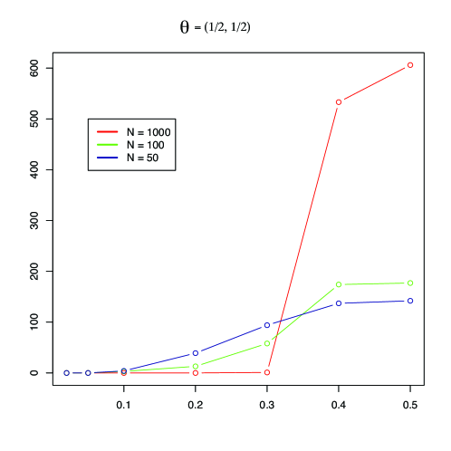
(c) From the practical point of view it is of interest to study the performance of the EM algorithm, for which no realistic global convergence guarantees are known; see [4] for a more detailed description of the problem. In our simulations to this end, we first generate our data in the same scenario as above with $\lambda_{1}=\lambda_{2}=\frac{1}{2}$, $\epsilon=0.1,\ldots,0.5$, and for sample sizes $N=50,100,1000$. We report how many times the EM algorithm was not able to find the global optimum in less than $10$ reruns. Given how simple and low-dimensional the model is, we think of $10$ reruns already as a big number. Our main findings are summarized in Figure 4. When the sample size is large ($N=1000$) this proportion is small if $\epsilon=0.02,0.05,0.1,0.2,0.3$. However, for higher $\epsilon$ in more than half cases the EM algorithm was not able to find the global optimum. If $N=50$ the results are even more interesting. Note that for $\epsilon=0.4,0.5$ the situation actually looks better than for $N=1000$. This is somewhat counterintuitive at first but easy to explain. High values of $\epsilon$ correspond to ill-behaved distributions (close to singularities). If $N$ is very high, the sample distribution lies close, and hence it is also ill-behaved, resulting in a complicated likelihood function. If the sample size is small, the variance of the sample distribution is much higher, so with relatively high probability the sample distribution will be far and better-behaved. In other words, if the correlations between variables are really small, smaller samples may lead to a better-behaved likelihood than big samples. For completeness of our discussion we repeat the same computations for a less symmetric set-up where $\lambda_{1}=\frac{1}{5}$ but the results were very similar and will not be reported here.

Figure 4. The numbers of non-convergers in the EM-algorithm for 1000 experiments and 10 reruns of the EM algorithm for each experiment depending on the parameters defining the data-generating distribution. The $x$-axis displays values of $\epsilon$.

4.4. EM attraction basins for $3\times 3\times 2$ tensors of $\text{rank}_{+}\leq 3$

We do not have a complete description of the boundary strata for tensors of nonnegative rank 3, nor formulas for MLEs. Thus, we present the results of our simulations for $3\times 3\times 2$ tensors with $\text{rank}_{+}\leq 3$, denoting the matrix parameters of appropriate format by $A$, $B$, and $C$. This model, denoted by $\mathcal{M}^{*}$, is a full-dimensional, proper subset of $\Delta_{17}$ (i.e. with Zariski closure the full ambient space as in the case of $\mathcal{M}_{3}$). We are interested in giving an estimate for the relative volume of $\mathcal{M}^{*}$ in $\Delta_{17}$ and in obtaining some preliminary understanding of attraction basins for distributions sampled from $\Delta_{17}$ under EM.

We performed two tests. For an arbitrary distribution $P\in\Delta_{17}$, we ran EM from ten different starting points, recorded the parameters $\theta_{0}\in\Theta$ to which EM converged, and took the optimal estimate. Without a full description of the boundary strata of $\mathcal{M}^{*}$, we classified the EM estimate into four categories: 1) the EM estimate $\theta_{0}$ contains strictly positive entries; 2) the EM estimate $\theta_{0}$ contains exactly one zero entry in a $3\times 3$ stochastic matrix; 3) the EM estimate $\theta_{0}$ contains exactly one zero entry in the $3\times 2$ stochastic matrix; 4) the EM estimate $\theta_{0}$ contains exactly $k$ zero entries for $k\in\{2,...,11\}$. The idea is that the numbers of EM estimates per category give approximations to which points of $\Theta$, either interior or on a boundary face of $\Theta$, the EM estimates are drawn. Concretely, these numbers are used to estimate respectively

1. the relative volume of $\mathcal{M}^{*}\subsetneq\Delta_{17}$;

2. the EM attraction basin proportion for the 6 irreducible components of the algebraic boundary given by a single zero in a $3\times 3$ stochastic matrix $A$ or $B$;

3. the EM attraction basin proportion for the 2 irreducible components of the algebraic boundary given by a single zero in the $3\times 2$ stochastic matrix $C$;

4. the EM attraction basin proportions for intersections of $k$ facets of $\Theta$.

For $10^{6}$ iterations, the proportions (given as percentages) of these EM attraction basins are given in Table 5, where $1a$-codim corresponds to the relative volume of category (2) and $1b$-codim to the relative volume of category (3). We separated categories (2) and (3), since (3) corresponds to a context specific independence model, but (2) does not.

We note that the highest concentration of estimates is in the faces of $\Theta$ of codimension $4$, though we have no insight as to why this is the case. Also the relative volume of $\mathcal{M}^{*}\subsetneq\Delta_{17}$, filling out only approximately $.019\%$ of $\Delta_{17}$ is remarkably small, particularly when compared to relative volume estimates for ${\mathcal{M}}_{3}$ and ${\mathcal{M}}_{3,3}$.

As a second test, we ran EM for the same $P\in\Delta_{17}$, but with $10^{4}$ different starting points. As expected, EM converged to many local optima on the nonconvex ${\mathcal{M}}^{*}$, with a majority (almost 76%) in the codim-4 stratum.

Table 5. Relative volume of EM attraction basins of strata in ${\mathcal{M}}^{*}$ using 10 different starting parameters for $10^{6}$ uniformly distributed points over $\Delta_{17}$.
 

$0$-codim	$1a$-codim	$1b$-codim	$2$-codim	$3$-codim	$4$-codim
0.019	0.2845	0.0621	3.4814	17.0098	40.1676

$5$-codim	$6$-codim	$7$-codim	$8$-codim	$9$-codim	$10$-codim	$11$-codim
25.7120	11.2486	1.7677	0.2249	0.0199	0.0025	0

5. EM fixed point ideals

It is well-known that the EM algorithm does not guarantee convergence to the global optimum of the likelihood function. In this section, we study the EM fixed point ideal introduced in [22] that eliminates this drawback. An EM fixed point for an observed data tensor $U$ is a parameter vector in $\Theta$ which stays fixed after one iteration of the EM algorithm. The set of EM fixed points includes the candidates for the global maxima of the likelihood function; see Lemma 24. The solution set of the EM fixed point ideal contains all the EM fixed points, in particular, all the global maxima of the likelihood function. Hence, computing the solution set of the EM fixed ideal allows the computation of all the global maxima for the likelihood function. Moreover, for a given model ${\mathcal{M}}$, the EM fixed point ideal consists of the equations defining all EM fixed points for any data tensor $U$. Therefore, for a given ${\mathcal{M}}$, it has to be computed only once. After this computationally intensive task, extracting the MLE for any given data tensor $U$ is relatively easy.

After first describing the equations of the EM fixed point ideal for ${\mathcal{M}}_{3}$ in Proposition 25, we present the full prime decomposition of this ideal in Theorem 26. We illustrate two uses of this decomposition. First, we show that using the components of the prime decomposition one can automatically recover the formulas for the maximum likelihood estimator for various strata that we presented in Section 4.2. Second, we point out that the relevant components of this decomposition that contain entries of stochastic parameter matrices correspond precisely to the boundary strata of ${\mathcal{M}}_{3}$, also reported in Section 4.2. This hints at the usefulness of the EM fixed point ideal for the discovery of such boundary strata. In fact, we showcase this discovery process by computing the decomposition of the EM fixed point ideal of ${\mathcal{M}}_{3,3}$. The components we get give the boundary stratification of ${\mathcal{M}}_{3,3}$ as reported in [29].

We present a version of the EM algorithm adapted to latent class models with three observed variables in Algorithm 1. We no longer assume that the observed or hidden variables are binary. We let $X_{1},X_{2},X_{3}$ be the observed random variables with $d_{1},d_{2},d_{3}$ states, respectively, and we assume that the hidden variable takes values in $\{1,\ldots,r\}$. We denote this model by ${\mathcal{M}}_{d_{1}\times d_{2}\times d_{3},r}$. Our presentation is based on [28, Section 1.3] and [22, Algorithm 1].

Input: Observed data tensor $U\in\mathbb{Z}^{d_{1}\times d_{2}\times d_{3}}$.

Output: A proposed maximum $\hat{P}\in\Delta_{d_{1}d_{2}d_{3}-1}$ of the log-likelihood function $\ell$ on the model $\mathcal{M}_{d_{1}\times d_{2}\times d_{3},r}$.

Step 0: Initialize randomly $(\lambda_{1},\ldots,\lambda_{r})\in\Delta_{r-1}$, $(a_{i1},\ldots,a_{id_{1}})\in\Delta_{d_{1}-1}$, $(b_{i1},\ldots,b_{id_{2}})\in\Delta_{d_{2}-1}$, and $(c_{i1},\ldots,c_{id_{3}})\in\Delta_{d_{3}-1}$ for $i=1,\ldots,r$.

Run the E-step and M-step until the entries of $P\in\Delta_{d_{1}d_{2}d_{3}-1}$ converge.

E-Step: Estimate the hidden data:

              Set $v_{lijk}:=\frac{\lambda_{l}a_{li}b_{lj}c_{lk}}{\sum_{l=1}^{r}\lambda_{l}a_{li}b_{lj}c_{lk}}u_{ijk}$ for $l=1,\ldots,r$, $i=1,\ldots,d_{1}$, $j=1,\ldots,d_{2}$, and $k=1,\ldots,d_{3}$.

M-Step: Maximize the log-likelihood function of the model with complete data using the estimates for the hidden data from the E-step:

              Set $\lambda_{l}:=\sum_{i=1}^{d_{1}}\sum_{i=1}^{d_{2}}\sum_{i=1}^{d_{3}}v_{ijkl}/u_{+++}$ for $l=1,...,r$.

              Set $a_{li}:=\sum_{j=1}^{d_{2}}\sum_{k=1}^{d_{3}}v_{ijkl}/(u_{+++}\lambda_{l})$ for $l=1,\ldots,r$, $i=1,\ldots,d_{1}$.

              Set $b_{lj}:=\sum_{i=1}^{d_{1}}\sum_{k=1}^{d_{3}}v_{ijkl}/(u_{+++}\lambda_{l})$ for $l=1,\ldots,r$, $j=1,\ldots,d_{2}$.

              Set $c_{lk}:=\sum_{i=1}^{d_{1}}\sum_{j=1}^{d_{2}}v_{ijkl}/(u_{+++}\lambda_{l})$ for $l=1,\ldots,r$, $k=1,\ldots,d_{3}$.

Update the joint distribution for the latent class model:

              Set $p_{ijk}:=\sum_{l=1}^{r}\lambda_{l}a_{li}b_{lj}c_{lk}$ for $i=1,\ldots,d_{1}$, $j=1,\ldots,d_{2}$, $k=1,\ldots,d_{3}$.

Return $P$.

Algorithm 1 EM algorithm for the latent class model with three observed variables

An EM fixed point for an observed data tensor $U$ is an element of $\Theta:=\Delta_{r-1}\times(\Delta_{d_{1}-1})^{r}\times(\Delta_{d_{2}-1})^{r}\times(\Delta_{d_{3}-1})^{r}$ which stays fixed after one E-step and M-step of the EM-algorithm with the input $U$.

Lemma 24.

Any $\theta\in\Theta$ to which the EM-algorithm can converge is an EM fixed point.

Proof.

Denote the function defined by one step of the EM-algorithm by $\operatorname{EM}(\cdot)$. Pick an initial point $\theta^{(0)}\in\Theta$, and let $\theta^{(k+1)}=\operatorname{EM}(\theta^{(k)})$. Assuming that $\theta:=\lim_{k\rightarrow\infty}\theta^{(k)}$ exists, then $\lim_{k}\theta^{(k+1)}=\lim_{k}\operatorname{EM}(\theta^{(k)})$, and since $\operatorname{EM}$ is continuous, we obtain $\theta=\operatorname{EM}(\theta)$. ∎

Lemma 24 justifies the study of the set of the EM fixed points as this set contains all possible outputs of the EM algorithm. In [22, Section 3], the set of all EM fixed points of a latent class model with two observed variables is studied through the minimal set of polynomial equations that they satisfy. These equations are called the EM fixed point equations.

Proposition 25.

The EM fixed point equations for $2\times 2\times 2$-tensors of rank${}_{+}\leq 2$ on the parameter space $\Theta$ are

$$a_{\ell i}\left(\sum_{j,k=1}^{2}r_{ijk}b_{\ell j}c_{\ell k}\right) =0\hskip 28.45274pt\mbox{ for all }\;\;\;\ell,i=1,2,$$

$$b_{\ell j}\left(\sum_{i,k=1}^{2}r_{ijk}a_{\ell i}c_{\ell k}\right) =0\hskip 28.45274pt\mbox{ for all }\;\;\;\ell,j=1,2,$$

$$c_{\ell k}\left(\sum_{i,j=1}^{2}r_{ijk}a_{\ell i}b_{\ell j}\right) =0\hskip 28.45274pt\mbox{ for all }\;\;\;\ell,k=1,2,$$

where $[r_{ijk}]=\left[u_{+++}-\frac{u_{ijk}}{p_{ijk}}\right]$.

Proof.

The proof is virtually identical to the proof of [22, Theorem 3.5]. ∎

We call the ideal generated by the equations in Proposition 25 the EM fixed point ideal and denote it by ${\mathcal{F}}$. This ideal is not prime and it defines a reducible variety. A minimal prime of ${\mathcal{F}}$ is called relevant if it contains none of the $8$ polynomials $p_{ijk}=\sum_{\ell=1}^{2}a_{\ell i}b_{\ell j}c_{\ell k}$ and none of the six ideals $\left\langle a_{l1},a_{l2}\right\rangle$, $\left\langle b_{l1},b_{l2}\right\rangle$ and $\left\langle c_{l1},c_{l2}\right\rangle$. Equivalently, an ideal is relevant, if not all of its solutions $P$ has a coordinate that is identically zero, and after normalizing the parameters, it comes from stochastic matrices.

Theorem 26.

The radical of the EM fixed point ideal ${\mathcal{F}}$ for ${\mathcal{M}}_{3}$ has precisely $63$ relevant primes consisting of $9$ orbital classes.

Proof.

This proof follows the proof of [22, Theorem 5.5] in using the approach of cellular components from [10]. The EM fixed point ideal ${\mathcal{F}}$ is given by

$$\left\langle a_{\ell i}\left(\sum_{j,k=1}^{2}r_{ijk}b_{\ell j}c_{\ell k}\right),b_{\ell j}\left(\sum_{i,k=1}^{2}r_{ijk}a_{\ell i}c_{\ell k}\right),c_{\ell k}\left(\sum_{i,j=1}^{2}r_{ijk}a_{\ell i}b_{\ell j}\right):i,j,k,l=1,2\right\rangle.$$

Any prime ideal containing ${\mathcal{F}}$ contains either $a_{\ell i}$ or $\sum_{j,k=1}^{2}r_{ijk}b_{\ell j}c_{\ell k}$ for $\ell,i\in\{1,2\}$, and either $b_{\ell j}$ or $\sum_{i,k=1}^{2}r_{ijk}a_{\ell i}c_{\ell k}$ for $\ell,j\in\{1,2\}$, and either $c_{\ell k}$ or $\sum_{i,j=1}^{2}r_{ijk}a_{\ell i}b_{\ell j}$ for $\ell,k\in\{1,2\}$. We categorize all primes containing ${\mathcal{F}}$ according to the set $S$ of parameters $a_{\ell i}$, $b_{\ell j}$, and $c_{\ell k}$ contained in them. The symmetry group acts on the parameters by permuting the rows of $A$, $B$, and $C$ simultaneously, the columns of $A$, $B$, and $C$ separately, and the matrices $A$, $B$, and $C$ themselves. For each orbit that consists of relevant ideals, we pick one representative $S$ and compute the cellular component ${\mathcal{F}}_{S}=(({\mathcal{F}}+\langle S\rangle):(\prod S^{c})^{\infty})$, where $S^{c}=\{a_{11},\ldots,a_{22},b_{11},\ldots,b_{22},c_{11},\ldots,c_{22}\}\setminus S$. Next we remove all representatives $S$ such that ${\mathcal{F}}_{T}\subset{\mathcal{F}}_{S}$ for a representative $T$ in another orbit. For each remaining cellular component ${\mathcal{F}}_{S}$, we compute its minimal primes. In each case, we use either the Macaulay2 minimalPrimes function or the linear elimination sequence from [13, Proposition 23(b)]. Finally, we remove those minimal primes of ${\mathcal{F}}_{S}$ that contain a cellular component ${\mathcal{F}}_{T}$ for a set $T$ (not necessarily a representative) in another orbit. The remaining $9$ minimal primes correspond to the rows of Table 6 and are uniquely determined by their properties. These are the set $S$, the degree and codimension, the ranks $rA=\text{rank}(A)$, $rB=\text{rank}(B)$, and $rC=\text{rank}(C)$ at a generic point. The $63$ ideals are obtained when counting each orbit with its orbit size in the last column of Table 6. ∎

Table 6. Minimal primes of EM fixed point ideal ${\mathcal{F}}$ for $2\times 2\times 2$-tensors of rank₊ 2.

Class S	$\mathbf{|S|}$	$a$’s	$b$’s	$c$’s	deg	codim	rA	rB	rC	orbit	type in Theorem 9
$\{\emptyset\}$	0	0	0	0	60	7	1	1	1	1	3-dimensional type 5
	0	0	0	0	48	7	2	2	1	1	4-dimensional type 4
	0	0	0	0	48	7	2	1	2	1	4-dimensional type 4
	0	0	0	0	48	7	1	2	2	1	4-dimensional type 4
	0	0	0	0	1	8	2	2	2	1	7-dimensional type 1
$\{a_{11}\}$	1	1	0	0	5	8	2	2	2	12	6-dimensional type 2
$\{a_{11},a_{22}\}$	2	2	0	0	25	8	2	2	2	6	5-dimensional type 3
$\{a_{11},b_{11}\}$	2	1	1	0	11	8	2	2	2	24	5-dimensional type 2
$\{a_{11},b_{11},c_{11}\}$	3	1	1	1	23	8	2	2	2	16	4-dimensional type 2

The rows of Table 6 correspond to different boundary strata in Theorem 9, and this correspondence is reported in the last column of the table. The orbit sizes in Table 6 are twice the number of corresponding strata in Corollary 10, except for the rows represented by $\{\emptyset\}$. This is because the ideal obtained by switching the rows of $A$, $B$ and $C$ is counted as distinct from the original ideal, though the tensors in the image of both sets of parameters are identical with parameters that differ only by label swapping. For example, the minimal prime represented by $\{a_{21}\}$ is one the 12 ideals in the orbit of the minimal prime represented by $\{a_{11}\}$, although $\{a_{11}=0\}$ and $\{a_{21}=0\}$ define the same boundary stratum.

In the next example we explain how to derive the EM fixed points and the potential MLEs from the former type of minimal primes of the EM fixed point ideal.

Example 1.

Consider the minimal prime of the EM fixed point ideal corresponding to $a_{11}=a_{22}=0$:

$$I_{1}= \langle a_{22},a_{11},r_{212}r_{221}-r_{211}r_{222},c_{11}r_{221}+c_{12}r_{222},b_{11}r_{212}+b_{12}r_{222},c_{11}r_{211}+c_{12}r_{212},$$

$$b_{11}r_{211}+b_{12}r_{221},r_{112}r_{121}-r_{111}r_{122},c_{21}r_{121}+c_{22}r_{122},b_{21}r_{112}+b_{22}r_{122},$$

$$c_{21}r_{111}+c_{22}r_{112},b_{21}r_{111}+b_{22}r_{121}\rangle.$$

We add to the ideal $I_{1}$ the ideal of the parametrization map

$$I_{2}= \langle-a_{21}b_{21}c_{21}+p_{111},-a_{21}b_{21}c_{22}+p_{112},-a_{21}b_{22}c_{21}+p_{121},-a_{21}b_{22}c_{22}+p_{122},$$

$$-a_{12}b_{11}c_{11}+p_{211},-a_{12}b_{11}c_{12}+p_{212},-a_{12}b_{12}c_{11}+p_{221},-a_{12}b_{12}c_{12}+p_{222}\rangle.$$

Eliminating parameters $a_{11},\ldots,c_{22}$ from $I_{1}+I_{2}$, gives the ideal

$$J= \langle p_{212}p_{221}-p_{211}p_{222},r_{221}p_{221}+r_{222}p_{222},r_{211}p_{221}+r_{212}p_{222},r_{212}p_{212}+r_{222}p_{222},$$

$$r_{211}p_{212}+r_{221}p_{222},r_{221}p_{211}+r_{222}p_{212},r_{212}p_{211}+r_{222}p_{221},r_{211}p_{211}-r_{222}p_{222},$$

$$p_{112}p_{121}-p_{111}p_{122},r_{121}p_{121}+r_{122}p_{122},r_{111}p_{121}+r_{112}p_{122},r_{112}p_{112}+r_{122}p_{122},$$

$$r_{111}p_{112}+r_{121}p_{122},r_{121}p_{111}+r_{122}p_{112},r_{112}p_{111}+r_{122}p_{121},r_{111}p_{111}-r_{122}p_{122},$$

$$r_{212}r_{221}-r_{211}r_{222},r_{112}r_{121}-r_{111}r_{122}\rangle$$

Finally, we substitute to the ideal $J$ the expressions

$$r_{ijk}=u_{+++}-\frac{u_{ijk}}{p_{ijk}}$$

and clear the denominators. To obtain an estimate for $p_{111}$, we eliminate all other $p_{ijk}$. This gives the ideal generated by $p_{111}u_{1++}u_{+++}-u_{11+}u_{1+1}$. Hence

$$p_{111}=\frac{u_{11+}u_{1+1}}{u_{1++}u_{+++}},$$

as in Section 4.

We used the method in Example 1 to verify the formulas in Section 4.2 for MLEs on different strata for all cases besides the $3$- and $4$-dimensional strata. For the $3$- and $4$-dimensional strata, the elimination of $p_{ijk}$’s did not terminate.

Since the rows of Table 6 are in correspondence with the boundary strata of ${\mathcal{M}}_{3}$, we believe that the method of decomposing the EM fixed point ideal is useful for identifying boundary strata for models whose geometry is not as well understood as that of ${\mathcal{M}}_{3}$. We illustrate this idea with the decomposition of ${\mathcal{M}}_{3,3}$.

Theorem 27.

The radical of the EM fixed point ideal ${\mathcal{F}}$ for ${\mathcal{M}}_{3,3}$ has $317$ relevant primes consisting of $21$ orbital classes. The properties of these orbital classes are listed in Table LABEL:r3.

Table 7. Minimal primes of EM fixed point ideal ${\mathcal{F}}$ for $2\times 2\times 2$-tensors of rank₊ 3.

Set S	$|S|$	$a$’s	$b$’s	$c$’s	deg	cdim	rA	rB	rC	orbit
$\{\emptyset\}$	0	0	0	0	121	10	1	1	1	1
	0	0	0	0	162	9	1	2	2	1
	0	0	0	0	162	9	2	1	2	1
	0	0	0	0	162	9	2	2	1	1
	0	0	0	0	38	10	2	2	2	$6\times 1$
	0	0	0	0	1	8	2	2	2	1
$\{a_{11}\}$	1	1	0	0	10	10	2	2	2	18
$\{a_{11},a_{21}\}$	2	2	0	0	5	9	2	2	2	18
$\{a_{11},b_{11}\}$	2	1	1	0	39	10	2	2	2	36
$\{a_{11},a_{21},a_{32}\}$	3	3	0	0	50	11	2	2	2	18
$\{a_{11},b_{11},c_{11}\}$	3	1	1	1	60	11	2	2	2	24
$\{a_{11},a_{21},b_{11},b_{21}\}$	4	2	2	0	11	10	2	2	2	36
$\{a_{11},a_{22},b_{11},b_{22}\}$	4	2	2	0	8	11	2	2	2	36
$\{a_{11},a_{21},b_{11},b_{21},c_{11},c_{21}\}$	6	2	2	2	23	11	2	2	2	24
$\{a_{11},a_{21},b_{11},b_{22},c_{11},c_{22}\}$	6	2	2	2	20	12	2	2	2	72
$\{a_{11},a_{22},b_{11},b_{22},c_{11},c_{22}\}$	6	2	2	2	23	12	2	2	2	24

Some of the ideals listed in Table LABEL:r3 have further constraints on the $3\times 2$ stochastic matrices $A$, $B$ and $C$ that cannot be read off directly from the table. These constraints are:

1. One out of the six ideals of degree $38$ corresponding to $\{\emptyset\}$ contains polynomials $a_{11}a_{22}-a_{12}a_{21}$, $b_{21}b_{32}-b_{22}b_{31}$ and $c_{11}c_{32}-c_{12}c_{31}$. Constraints for the rest of the five ideals are obtained by permuting simultaneously the rows of $A$, $B$ and $C$.

2. The ideal corresponding to $\{a_{11}\}$ contains polynomials $b_{21}b_{32}-b_{22}b_{31}$ and $c_{21}c_{32}-c_{22}c_{31}$.

3. The ideal corresponding to $\{a_{11},b_{11}\}$ contains the polynomial $c_{21}c_{32}-c_{22}c_{31}$.

4. The ideal corresponding to $\{a_{11},a_{21},a_{32}\}$ contains polynomials $b_{11}b_{22}-b_{12}b_{21}$ and $c_{11}c_{22}-c_{12}c_{21}$.

5. The ideal corresponding to $\{a_{11},b_{11},c_{11}\}$ contains polynomials $a_{21}a_{32}-a_{22}a_{31}$, $b_{21}b_{32}-b_{22}b_{31}$ and $c_{21}c_{32}-c_{22}c_{31}$.

The semialgebraic description, boundary stratification and closed formulas for MLEs for ${\mathcal{M}}_{3,3}$ are obtained in [29]. The boundary stratification poset for ${\mathcal{M}}_{3,3}$ agrees with the one for ${\mathcal{M}}_{3}$ in Figure 3. The parameters that yield different types of boundary strata for ${\mathcal{M}}_{3,3}$ are included in Table LABEL:r3:

1. Interior: $\{\emptyset\}$ ($A,B,C$ rank $2$, no further constraints on $A$, $B$ and $C$).

2. Codimension 1 strata: $\{a_{11}\}^{*}$, $\{a_{11},a_{21}\}$.

3. Exceptional codimension 2 strata: $\{a_{11},a_{21},a_{32}\}^{*}$.

4. Codimension 2 strata: $\{a_{11},b_{11}\}^{*}$, $\{a_{11},a_{21},b_{11},b_{21}\}$.

5. Exceptional codimension 3 strata: $\{\emptyset\}^{*}$ ($A$, $B$ or $C$ rank $1$).

6. Codimension 3 strata: $\{a_{11},b_{11},c_{11}\}^{*}$, $\{a_{11},a_{21},b_{11},b_{21},c_{11},c_{21}\}$.

7. Unique codimension 4 stratum: $\{\emptyset\}^{*}$ ($A$, $B$ and $C$ rank $1$).

8. Other: $\{\emptyset\}^{*}$ ($A,B,C$ rank $2$, further constraints on $A$, $B$ and $C$), $\{a_{11},a_{22},b_{11},b_{22}\}$, $\{a_{11},a_{21},b_{11},b_{22},c_{11},c_{22}\}$, $\{a_{11},a_{22},b_{11},b_{22},c_{11},c_{22}\}$.

A star indicates that besides setting the elements in the set to zero, further equation constraints on the parameters (either rank constraints from Table LABEL:r3 or other constraints from the list above) are needed to define the stratum. Taking these further constraints into account, for a fixed type of boundary stratum, all parametrizations from Table LABEL:r3 are minimal. All the rows of Table LABEL:r3 that do not give boundary strata lie on the singular locus of ${\mathcal{M}}_{3,3}$.

References

- [1] Elizabeth S. Allman, Catherine Matias, and John A. Rhodes. Identifiability of parameters in latent structure models with many observed variables. Ann. Statist., 37(6A):3099–3132, 2009.
- [2] Elizabeth S. Allman, John A. Rhodes, Bernd Sturmfels, and Piotr Zwiernik. Tensors of nonnegative rank two. Linear Algebra Appl., 473:37–53, 2015.
- [3] Elizabeth S. Allman, John A. Rhodes, and Amelia Taylor. A semialgebraic description of the general Markov model on phylogenetic trees. SIAM J. Discrete Math., 28(2):736–755, 2014.
- [4] Sivaraman Balakrishnan, Martin J. Wainwright, and Bin Yu. Statistical guarantees for the EM algorithm: From population to sample-based analysis. Ann. Statist., 45(1):77–120, 02 2017.
- [5] Christopher M. Bishop. Pattern recognition and machine learning. Information Science and Statistics. Springer, New York, 2006.
- [6] Craig Boutilier, Nir Friedman, Moises Goldszmidt, and Daphne Koller. Context-specific independence in bayesian networks. In Proceedings of the Twelfth international conference on Uncertainty in artificial intelligence, pages 115–123. Morgan Kaufmann Publishers Inc., 1996.
- [7] Fabrizio Catanese, Serkan Hoşten, Amit Khetan, and Bernd Sturmfels. The maximum likelihood degree. Amer. J. Math., 128(3):671–697, 2006.
- [8] Vin de Silva and Lek-Heng Lim. Tensor rank and the ill-posedness of the best low-rank approximation problem. SIAM J. Matrix Anal. Appl., 30(3):1084–1127, 2008.
- [9] A. P. Dempster, N. M. Laird, and D. B. Rubin. Maximum likelihood from incomplete data via the EM algorithm. J. Roy. Statist. Soc. Ser. B, 39(1):1–38, 1977. With discussion.
- [10] David Eisenbud and Bernd Sturmfels. Binomial ideals. Duke Mathematical Journal, 84(1):1–45, 1996.
- [11] Stephen E. Fienberg. Discussion on the paper by Dempster, Laird, and Rubin. J. Roy. Statist. Soc. Ser. B, 39(1):29–30, 1977.
- [12] Stephen E. Fienberg, Patricia Hersh, Alessandro Rinaldo, and Yi Zhou. Maximum likelihood estimation in latent class models for contingency table data. In Algebraic and geometric methods in statistics, pages 27–62. Cambridge Univ. Press, Cambridge, 2010.
- [13] Luis David Garcia, Michael Stillman, and Bernd Sturmfels. Algebraic geometry of Bayesian networks. J. Symbolic Comput., 39(3-4):331–355, 2005.
- [14] Francisca Galindo Garre and Jeroen K Vermunt. Avoiding boundary estimates in latent class analysis by Bayesian posterior mode estimation. Behaviormetrika, 33(1):43–59, 2006.
- [15] Dan Geiger, David Heckerman, Henry King, and Christopher Meek. Stratified exponential families: graphical models and model selection. Annals of Statistics, pages 505–529, 2001.
- [16] Zvi Gilula. Singular value decomposition of probability matrices: Probabilistic aspects of latent dichotomous variables. Biometrika, 66(2):339–344, 1979.
- [17] Leo A. Goodman. On the estimation of parameters in latent structure analysis. Psychometrika, 44(1):123–128, Mar 1979.
- [18] Shelby J. Haberman. Log-linear models for frequency tables derived by indirect observation: maximum likelihood equations. Ann. Statist., 2:911–924, 1974.
- [19] Serkan Hoşten, Amit Khetan, and Bernd Sturmfels. Solving the likelihood equations. Found. Comput. Math., 5(4):389–407, 2005.
- [20] Joseph B. Kruskal. More factors than subjects, tests and treatments: an indeterminacy theorem for canonical decomposition and individual differences scaling. Psychometrika, 41(3):281–293, 1976.
- [21] Joseph B. Kruskal. Three-way arrays: rank and uniqueness of trilinear decompositions, with application to arithmetic complexity and statistics. Linear Algebra and Appl., 18(2):95–138, 1977.
- [22] Kaie Kubjas, Elina Robeva, and Bernd Sturmfels. Fixed points EM algorithm and nonnegative rank boundaries. Ann. Statist., 43(1):422–461, 2015.
- [23] Steffen L. Lauritzen. Graphical models, volume 17 of Oxford Statistical Science Series. The Clarendon Press, Oxford University Press, New York, 1996. Oxford Science Publications.
- [24] Paul F. Lazarsfeld. The logical and mathematical foundation of latent structure analysis. Studies in Social Psychology in World War II Vol. IV: Measurement and Prediction, pages 362–412, 1950.
- [25] Paul F. Lazarsfeld and Neil W. Henry. Latent Structure Analysis. Houghton, Mifflin, New York, 1968.
- [26] Richard B McHugh. Efficient estimation and local identification in latent class analysis. Psychometrika, 21(4):331–347, 1956.
- [27] Mateusz Michałek, Luke Oeding, and Piotr Zwiernik. Secant cumulants and toric geometry. International Mathematics Research Notices, 2015(12):4019–4063, 2015.
- [28] Lior Pachter and Bernd Sturmfels. Algebraic statistics for computational biology, volume 13. Cambridge university press, 2005.
- [29] Anna Seigal and Guido Montúfar. Mixtures and products in two graphical models. J. Algebraic Statistics. to appear.