Suppression of the overlap between Majorana fermions by orbital magnetic effects in semiconducting-superconducting nanowires

Abstract

We study both analytically and numerically the role of orbital effects caused by a magnetic field applied along the axis of a semiconducting Rashba nanowire in the topological regime hosting Majorana fermions. We demonstrate that the orbital effects can be effectively taken into account in a one-dimensional model by shifting the chemical potential, and, thus modifying the topological criterion. We focus on the energy splitting between two Majorana fermions in a finite nanowire and find a striking interplay between orbital and Zeeman effects on this splitting. In the limit of strong spin-orbit interaction, we find regimes where the amplitude of the oscillating splitting stays constant or even decays with increasing magnetic field, in stark contrast to the commonly studied case where orbital effects of the magnetic field are neglected. The period of these oscillations is found to be almost constant in many parameter regimes.

Introduction. Majorana fermions (MFs) in condensed matter systems have been at the center of attention over many years. They have been predicted to emerge in such systems as semiconducting nanowires alicea2010majorana ; lutchyn2010majorana ; oreg2010helical ; gangadharaiah2011majorana ; sticlet2012spin ; rainis2013towards ; maier2014majorana ; sarma2012splitting ; dominguez2012dynamical ; klinovaja2012transition ; prada2012transport ; leijnse2012introduction ; nakosai2013majorana ; reeg2014zero ; bjornson2013vortex ; weithofer2014electron ; dmytruk2015cavity , $p$-wave superconductors brouwer2011probability ; degottardi2013majorana ; thakurathi2015majorana ; scharf2015probing , graphene-like systems klinovaja2012electric ; klinovaja2012helical ; klinovaja2013giant ; Dutreix2014 ; klinovaja2013spintronics ; black2012edge ; san2015majorana ; zhou2016ising ; kaladzhyan2017formation , and chains of magnetic atoms nadj2013proposal ; klinovaja2013topological ; braunecker2013interplay ; vazifeh2013self ; pientka2013topological ; poyhonen2014majorana , with some of these proposals implemented experimentally mourik2012signatures ; das2012zero ; deng2012anomalous ; churchill2013superconductor ; albrecht2016exponential ; nadj2014observation ; ruby2015end ; pawlak2016probing ; rokhinson2012fractional ; saldana2017electric . In this work, we focus on Rashba nanowire setups lutchyn2010majorana ; oreg2010helical , which have been widely implemented experimentally mourik2012signatures ; das2012zero ; deng2012anomalous ; churchill2013superconductor ; albrecht2016exponential . The experimental evidence of MFs in semiconducting nanowires is based on the observation of emerging zero-bias peaks in the differential conductance as a function of magnetic field applied along the nanowire axis mourik2012signatures ; das2012zero ; deng2012anomalous ; churchill2013superconductor .

However, at large magnetic fields MFs initially localized at two opposite nanowire ends overlap, resulting in finite-energy fermionic states prada2012transport ; rainis2013towards ; sarma2012splitting ; maier2014majorana . So far, theoretical works have predicted that the energy of these fermionic states should grow exponentially with increasing magnetic field, up to the point where these bound states have crossed the gap and merge with the bulk states prada2012transport ; sarma2012splitting ; rainis2013towards ; maier2014majorana . In contrast to that, transport measurements performed on such nanowires reported the observation of constant or decreasing energy splitting of the MFs as a function of magnetic field churchill2013superconductor ; albrecht2016exponential , which was often used as an argument against MF interpretation of such data liu2017phenomenology .

In this work, we resolve this paradox between theory and experiment by taking into account orbital magnetic effects neglected so far and study their effect on the MF energy splitting. In reality, nanowires have a finite diameter, indicating that orbital effects of the magnetic field may be important. We will show that properly accounting for such orbital effects may explain constant or decreasing amplitude of the MF splitting oscillations in the topological phase. Numerical studies of the topological phase diagram taking into account orbital effects are reported for cylindrical and hexagonal nanowires lim2013emergence ; nijholt2016orbital . However, so far, not much attention has been paid to the importance of orbital effects for characterization of the energy splitting between MFs.

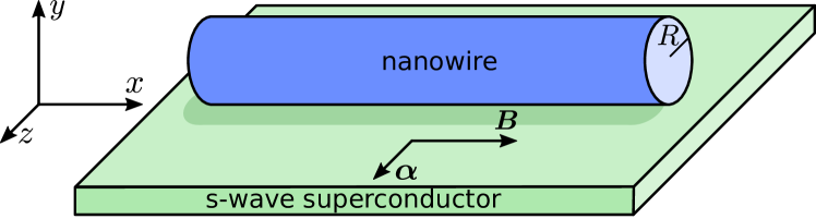
Figure 1: The setup consists of the semiconductor Rashba nanowire of radius $R$ brought into proximity to an $s$-wave bulk superconductor. The nanowire is aligned along the $\hat{x}$ axis and the SOI vector $\boldsymbol{\alpha}$ is along the $\hat{z}$ axis. An external magnetic field $\boldsymbol{B}$ applied along the nanowire, i.e along the $\hat{x}$ axis, drives the setup into the topological phase hosting MFs localized at the nanowire ends.

In this paper, we propose a one-dimensional (1D) model that takes into account the orbital effects caused by the magnetic field and study how they modify the topological phase. Our system consists of a semiconducting nanowire with Rashba spin-orbit interaction (SOI) in proximity to an $s$-wave bulk superconductor (see Fig. 1). By applying a magnetic field, such a system can be brought into the topological phase with MFs emerging at the ends of the nanowire. Typically in experiments, the magnetic field is applied along the nanowire axis ($\hat{x}$) in order not to destroy the bulk superconductivity, while the Rashba SOI is orthogonal to the magnetic field $B$ (chosen here along $\hat{z}$). In most theoretical works, the magnetic field is assumed to enter only as a Zeeman term, while the orbital contribution is dismissed due to the small nanowire diameter. As a result, MF oscillations have been found only in the weak SOI regime, where the Fermi wavevector depends on $B$, and thus the amplitude of the splitting always grows as the localization length grows with increasing $B$-field prada2012transport ; sarma2012splitting ; rainis2013towards ; maier2014majorana . In the strong SOI regime fasth2007direct ; nadj2012spectroscopy ; van2015spin ; kammhuber2017conductance , the Fermi wavevector is independent of $B$ unless orbital effects, shifting the chemical potential, are taken into account. The dominant MF localization length, determined by the proximity gap at the exterior branches of the wire spectrum, stays constant in this regime, so one expects a constant amplitude of the MF overlap. We demonstrate that, quite remarkably, these orbital effects can qualitatively change the MF energy splitting and thus can account for a better agreement between theory and recent experiments albrecht2016exponential .

Orbital effects in lowest subbands. A three-dimensional nanowire is described by the Hamiltonian $H_{3D}(x,y,z)$ in which the dynamics along the nanowire ($\hat{x}$-axis) and in the cross-section of the nanowire ($\hat{y}\hat{z}$-plane) are independent, $H_{3D}(x,y,z)=\bar{H}(x)+H_{2D}(y,z)$. As a result, the wavefunction takes the form $\Psi(x,y,z)=\bar{\Psi}(x)\Psi_{2D}(y,z)$ and the problem can be solved in two steps. Thus, we first focus on finding the eigenvalues of $H_{2D}(y,z)$ in the presence of orbital effects. Afterwards, we deal with the effective one-dimensional model, in which the chemical potential $\mu$ shifts as a function of the magnetic field. Below, we show that at small magnetic fields the dependence is quadratic, so $\mu=\mu_{0}-\overline{\beta}\left(\Phi/\Phi_{0}\right)^{2}$, where $\Phi_{0}=hc/e$, $\mu_{0}$ is the initial chemical potential, $\Phi=BS$ is the magnetic flux through the nanowire cross-section of area $S$.

The simplest model to consider analytically is a cylindrical hollow nanowire of radius $R$  lim2013emergence ; winkler2017orbital . The kinetic term in the transverse direction is written in polar coordinates (in $\hat{y}\hat{z}$ plane, see Fig. 1) as

$$H_{kin}^{cyl}=\int d\phi\ \psi^{\dagger}(\phi)\dfrac{\hbar^{2}}{2m^{*}}\left(\dfrac{-i\partial_{\phi}}{R}-\dfrac{eBR}{2c\hbar}\right)^{2}\psi(\phi),$$ (1)

where $m^{*}$ is the effective mass and the vector potential $A=BR/2$ is chosen in the Coulomb gauge. The energy spectrum is given by $E_{l}^{cyl}=\hbar^{2}\left(l-\Phi/\Phi_{0}\right)^{2}/2m^{*}R^{2}$, where $\Phi=\pi R^{2}B$ is the magnetic flux through the cylinder cross-section and the quantum number $l$ corresponding to the angular momentum is an integer. In what follows, we work with the lowest non-degenerate subband ($l=0$), so the orbital effects indeed could be taken into account by shifting the chemical potential up proportionally to $B^{2}$, where the corresponding coefficient is defined as $\bar{\beta}^{cyl}=\hbar^{2}/2m^{*}R^{2}$ (see above).

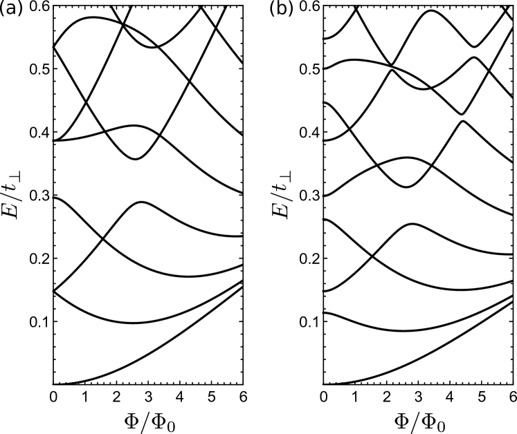
Figure 2: The energy spectrum of the nanowire with the cross-section $N_{y}a\times N_{z}a$ as a function of the magnetic flux $\Phi/\Phi_{0}$. (a) In a nanowire with a square cross-section ($N_{y}\times N_{z}=12\times 12$), the lowest energy level is non-degenerate, while the majority of higher subbands is two-fold degenerate at $B=0$ due to the additional mirror symmetry. (b) In contrast to that, in a nanowire with a rectangular cross-section ($N_{y}\times N_{z}=14\times 12$) the symmetry is broken and, as a result, lowest subbands are non-degenerate. In both cases, the bottom of the lowest subband moves up as a quadratic function of $B$. One flux quantum through the cross-section corresponds to magnetic fields of strength (a) $B=0.41~{}T$ or (b) $B=0.35~{}T$ for $a=8.33~{}\text{nm}$. The splitting between subbands is determined by $t_{\perp}=\hbar^{2}/2m^{*}a^{2}=37$ meV, where $m^{*}=0.015m_{e}$.

Next, we study numerically a more realistic situation in which a nanowire has a rectangular cross section $N_{y}a\times N_{z}a$, where $a$ is the effective lattice constant. In the Landau gauge $\vec{A}=By\hat{z}$, the tight-binding Hamiltonian reads as

$$H_{2D}= -t_{\perp}\sum_{j=1}^{N_{y}}\sum_{k=1}^{N_{z}+1}c^{\dagger}_{j+1,k}c_{j,k}$$ (2)

$$\hskip 35.0pt-t_{\perp}\sum_{j=1}^{N_{y}+1}\sum_{k=1}^{N_{z}}e^{-i\varphi_{j}}c^{\dagger}_{j,k+1}c_{j,k}+{\rm H.c.},$$

where the phase $\varphi_{j}=2\pi\Phi j/\left(N_{y}N_{z}\Phi_{0}\right)$ accounts for orbital effects, $\Phi=BN_{y}N_{z}a^{2}$ is the magnetic flux though the nanowire cross-section, and $t_{\perp}>0$ is the hopping amplitude. Here, $c_{j,k}^{\dagger}(c_{j,k})$ is the fermionic creation (annihilation) operator at site $(j,k)$ of the square lattice.

In nanowires with a square cross-section $N_{y}=N_{z}$, the lowest subband is non-degenerate, while the majority of higher subbands are multiply degenerate at $B=0$ due to the presence of an additional mirror plane going through the square diagonal and the nanowire axis, see Fig. 2(a). This degeneracy should be expected to occur in all nanowires with high-symmetry cross-sections. However, in presence of disorder or working with nanowires covered only partially by the superconductor, we assume such symmetries are broken and the degeneracy is lifted. For example, if $N_{y}$ and $N_{z}$ are non-commensurable, the lowest energy subbands are non-degenerate [see Fig. 2(b)]. Again, for small magnetic fields the bottom of the lowest subband moves up as $\propto B^{2}$, which is consistent with results obtained for hollow cylinders saldana2017electric . We note that also the lowest energy levels of the Fock–Darwin spectrum for an electron in a parabolic 2D confinement subjected to small magnetic fields follows the same dependence on the flux geerinckx1990effect ; madhav1994electronic ; burkard1999coupled ; tsitsishvili2004rashba . In what follows, we focus on this case of a single non-degenerate band and take into account orbital effects via an effective shift of the chemical potential.

Effective 1D Hamiltonian. Next, we introduce an effective continuum model for a one-dimensional Rashba nanowire described by the Hamiltonian $H=H_{kin}+H_{so}+H_{Z}+H_{SC}$, where

$$H_{kin}=\sum_{\sigma}\int dx\ \psi^{\dagger}_{\sigma}(x)\left[-\hbar^{2}\partial^{2}_{x}/2m^{*}-\mu\right]\psi_{\sigma}(x),$$ (3)

$$H_{so}=-i\alpha\sum_{\sigma,\sigma^{\prime}}\int dx\ \psi^{\dagger}_{\sigma}(x)\left(\sigma_{z}\right)_{\sigma\sigma^{\prime}}\partial_{x}\psi_{\sigma^{\prime}}(x),$$ (4)

$$H_{Z}=V_{Z}\sum_{\sigma,\sigma^{\prime}}\int dx\ \psi^{\dagger}_{\sigma}(x)\left(\sigma_{x}\right)_{\sigma\sigma^{\prime}}\psi_{\sigma^{\prime}}(x),$$ (5)

$$H_{SC}=\dfrac{\Delta}{2}\sum_{\sigma,\sigma^{\prime}}\int dx\ \psi_{\sigma}(x)\left(i\sigma_{y}\right)_{\sigma\sigma^{\prime}}\psi_{\sigma^{\prime}}(x)+H.c.$$ (6)

with $\alpha$ being the SOI strength, $\Delta$ the proximity-induced pairing gap, $V_{Z}=g\mu_{B}B/2$ the Zeeman energy, where $g$ is the $g$-factor of the nanowire and $\mu_{B}$ the Bohr magneton. Here, $\psi^{\dagger}_{\sigma}(x)\left[\psi_{\sigma}(x)\right]$ is the creation (annihilation) operator of an electron at position $x$ with spin $\sigma/2=\pm 1/2$, and $\sigma_{x,y,z}$ are the Pauli matrices acting on the spin of the electron. We assume $V_{Z}$ and $\Delta$ to be positive without loss of generality.

Topological criterion modified by orbital effects. The topological phase transition is associated with a closing and reopening of the bulk gap. The Rashba nanowire is in the topological phase with MFs appearing at both ends of the nanowire if $V_{Z}>\sqrt{\mu_{0}^{2}+\Delta^{2}}\equiv V_{Z}^{0}$, where the chemical potential $\mu_{0}$ is calculated from the SOI energy lutchyn2010majorana ; oreg2010helical . Orbital magnetic effects taken into account in the effective model as $\mu=\mu_{0}-\beta V_{Z}^{2}$ [$\beta=\bar{\beta}\left(2S/g\mu_{B}\Phi_{0}\right)^{2}$] modify the topological criterion. In particular, as the magnetic field is increased, the Zeeman energy grows, however, at the same time the bottom of the subband moves up and the chemical potential is decreasing, which makes it more difficult to achieve the topological phase. In particular, if the initial potential is too low, $\mu_{0}<-1/2\beta$ or $\mu_{0}<(4\beta^{2}\Delta^{2}-1)/4\beta$, the system is always in the trivial phase. Generally, there are two critical values of magnetic fields $V_{Z,\pm}$ at which the gap at $k=0$ closes,

$$V_{Z,\pm}^{2}=(1+2\beta\mu_{0}\pm\sqrt{1+4\beta\mu_{0}-4\beta^{2}\Delta^{2}})/2\beta^{2},$$ (7)

and, thus, the topological phase transition takes place twice. The topological phase hosting MFs at each end of the nanowire described by the modified topological criterion $V_{Z,-}<V_{Z}<V_{Z,+}$. In the limit $\beta\to 0$, we reproduce the standard topological criterion $V_{Z-}=V_{Z}^{0}$ and $V_{Z+}$ diverges. If after the first topological phase transition, the magnetic field is increased further, the system could be driven out of the topological phase again (see Fig. 3). In particular, in sufficiently long nanowires, one will observe that the zero-bias MF peak in the conductance disappears without showing any oscillations mourik2012signatures . Moreover, as it is difficult to detect the closing of the bulk gap in the nanowires with a soft superconducting gap via transport measurements, the sudden disappearance of MFs could look puzzling, if orbital effects are not taken into account. For $(1-\sqrt{1-\beta^{2}\Delta^{2}})/\beta<\mu_{0}<(1+\sqrt{1-\beta^{2}\Delta^{2}})/\beta$, $V_{z-}$ is smaller than $V_{Z}^{0}$ and the topological phase is achieved at smaller magnetic fields. In addition, due to orbital effects, the topological phase shifts towards higher values of chemical potential, which reduces the challenging requirement of tuning the electron density to very low values.

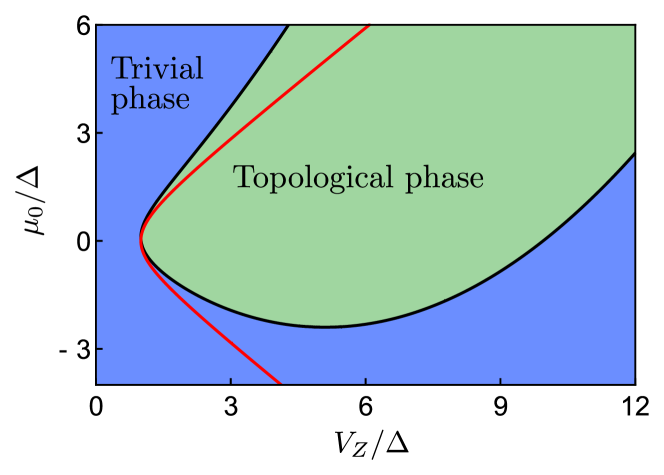
Figure 3: Topological phase diagram as a function of applied magnetic field in units of $V_{Z}/\Delta$ and of initial chemical potential $\mu_{0}/\Delta$ for $\beta\Delta=0.1$. The topological (green area) and trivial (blue area) phases are separated by the phase boundary (black line) corresponding to the closing of the bulk gap. The red line indicates the phase boundary in the absence of orbital effects. Clearly, orbital effects are responsible for shifting the topological phase to higher values of chemical potentials.

MF wavefunctions: semi-infinite nanowire. After, we have identified the bulk properties, we will focus on MFs in semi-infinite nanowires. To find the MF wavefunctions, we consider the strong SOI regime defined by the condition that the SOI energy is the largest energy scale, $E_{so}=\hbar^{2}k_{so}^{2}/2m^{*}\gg V_{Z},\Delta,\mu$, where $k_{so}=m^{*}\alpha/\hbar^{2}$. In this regime, we linearize the Hamiltonian $H$ near the Fermi points $k^{(i)}_{F}=0$ ($k_{F}^{(e)}=\pm 2k_{so}$) corresponding to the interior (exterior) branch of the spectrum with the Fermi velocity $\upsilon_{F}=\alpha/\hbar$ by expressing the electron operators $\psi_{\sigma}(x)$ in terms of slowly varying left $L_{\sigma}$ and right $R_{\sigma}$ movers braunecker2010spin ; klinovaja2012composite ; klinovaja2012transition , $\psi_{\uparrow}(x)=R_{\uparrow}(x)+e^{-2ik_{so}x}L_{\uparrow}(x)$ and $\psi_{\downarrow}(x)=e^{2ik_{so}x}R_{\downarrow}(x)+L_{\downarrow}(x)$. Next, we construct the basis vector that corresponds to the exterior (interior) branch $\left(\phi^{e}\right)^{T}$ = ($L_{\uparrow}$, $R_{\downarrow}$, $L^{\dagger}_{\uparrow}$, $R^{\dagger}_{\downarrow}$) [$\left(\phi^{i}\right)^{T}$ = ($R_{\uparrow}$, $L_{\downarrow}$, $R^{\dagger}_{\uparrow}$, $L^{\dagger}_{\downarrow}$)]. The linearized Hamiltonian density, $\tilde{H}^{l}=\frac{1}{2}\int dx\ \left[\phi^{l}(x)\right]^{\dagger}\mathcal{H}^{l}\phi^{l}(x)$, can be written in terms of Pauli matrices $\eta_{x,y,z}$ acting on the electron-hole subspace as

$$\mathcal{H}^{e}=i\hbar\upsilon_{F}\sigma_{z}\partial_{x}+\Delta\sigma_{y}\eta_{y}-\mu\eta_{z},$$

$$\mathcal{H}^{i}=-i\hbar\upsilon_{F}\sigma_{z}\partial_{x}+V_{Z}\sigma_{x}\eta_{z}+\Delta\sigma_{y}\eta_{y}-\mu\eta_{z}.$$ (8)

Imposing vanishing boundary conditions at the left end of the nanowire, we find $\Psi_{L}(x)=(f,if^{*},f^{*},-if)^{T}/\sqrt{\mathcal{N}}$ with

$$f(x)=\left(-ie^{i\left(2k_{so}-\mu/\alpha\right)x-x/\xi^{e}}+ie^{-x/\xi^{i}}\right)e^{-i\varphi_{L}/2},$$ (9)

where $\mathcal{N}$ is the normalization prefactor and $\sin\varphi_{L}=\mu/V_{Z}$. The MF localization lengths are given by $\xi^{e}=\alpha/\Delta$ and $\xi^{i}=\alpha/\left(\sqrt{V_{Z}^{2}-\mu^{2}}-\Delta\right)$. By analogy, we also find the MF wavefunction localized at the right end of the nanowire and, thus, exponentially decaying to the left, let say, for $x<L$ with $\Psi_{R}(x=L)=0$. Not surprisingly, the left and right MF wavefunctions are related as $\Psi_{R}(x)=\Psi_{L}^{*}(L-x)$, reflecting the mirror symmetry between the two ends.

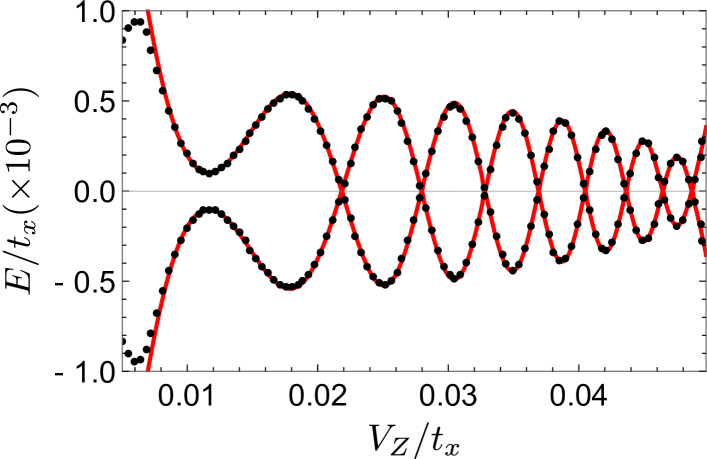
Figure 4: The MF energy splitting as a function of applied magnetic field in units of $V_{Z}/t_{x}$ obtained by numerical diagonalization (red solid line) or using the analytical expression for $\delta\epsilon$ (black dotted line). The overlap between MFs decays and exhibits oscillations with almost constant period. The used parameters are $N=300$, $\Delta/t_{x}=0.005$, $\mu=-20V_{Z}^{2}/t_{x}$ and $\overline{\alpha}/t_{x}=0.3$.

Tight-binding model. Next, we would like to focus on the finite-size nanowires and calculate the splitting between two MFs. To achieve this, we first turn to the modeling of the system by using the tight-binding Hamiltonian of a 1D chain composed of $N+1$ sites rainis2013towards ; klinovaja2015fermionic

$$\overline{H}=\sum_{\sigma,\sigma^{\prime}}\sum_{j=1}^{N}c^{\dagger}_{j+1,\sigma}\Big{[}i\overline{\alpha}\sigma^{z}_{\sigma\sigma^{\prime}}-t_{x}\delta_{\sigma\sigma^{\prime}}\Big{]}c_{j,\sigma^{\prime}}-\sum_{j=1}^{N+1}\Delta c^{\dagger}_{j,\uparrow}c^{\dagger}_{j,\downarrow}$$

$$-\sum_{\sigma,\sigma^{\prime}}\sum_{j=1}^{N+1}c^{\dagger}_{j,\sigma}\Big{[}\left(\mu-2t_{x}\right)\delta_{\sigma\sigma^{\prime}}-V_{Z}\sigma^{x}_{\sigma\sigma^{\prime}}\Big{]}c_{j,\sigma^{\prime}}+{\rm H.c.},$$ (10)

where $c_{j,\sigma}^{\dagger}(c_{j,\sigma})$ is the creation (annihilation) operator acting on electrons with spin $\sigma$ located at site $j$. Here, $t_{x}=\hbar^{2}/\left(2m^{*}a_{x}^{2}\right)$ is the hopping amplitude along $\hat{x}$, with $a_{x}$ being the lattice constant, and $\overline{\alpha}$ is the spin-flip hopping amplitude, related to the SOI parameter by $\overline{\alpha}=\alpha/2a_{x}$.

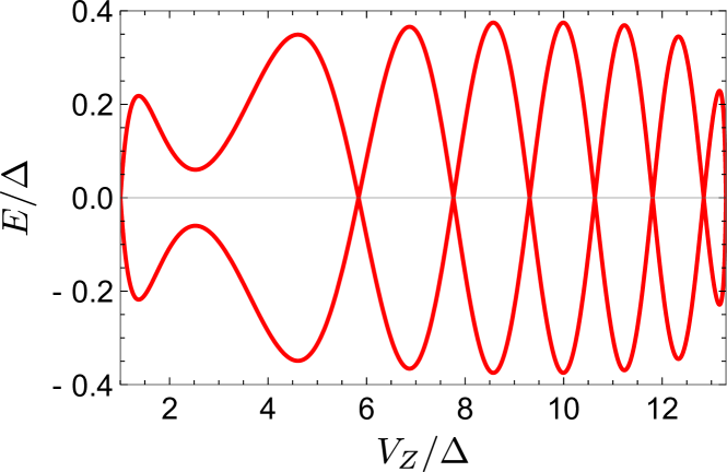
Figure 5: The MF energy splitting as a function of applied magnetic field in units of $V_{Z}/\Delta$ in finite-size nanowire $k_{so}L=151$. The amplitude of oscillations stays constant away from the topological phase transition points, close to which it shrinks. The parameters are chosen as $E_{so}/\Delta=50$ and $\mu=-0.075V_{Z}^{2}/\Delta$.

Splitting between MFs. Next, we focus on the splitting between MFs. Numerically, we find that the amplitude of MF splitting either stays constant or decays, see Fig. 4. The left and right MF wavefunctions found independently for a semi-infinite nanowire do not satisfy the Schrödinger equation if the nanowire length is finite. Using perturbation theory we find that the degeneracy between the two MF levels is lifted by $\delta\epsilon=\left|\left\langle 0\left|\gamma_{R}\overline{H}\gamma_{L}^{\dagger}\right|0\right\rangle\right|$, where $\gamma_{L,R}$ are MF operators (the details of the derivation are presented in the SM SM ). In the regime of strong SOI, $\delta\epsilon$ can be simplified as

$$\delta\epsilon\approx\frac{2\hbar\upsilon_{F}}{\xi^{e}+\xi^{i}}\left|f\left(L\right)\right|\left|\sin\left(\tilde{\varphi}\right)\right|,$$ (11)

where $\tilde{\varphi}=\varphi_{L}/2-\text{Arg}\left[f(L)\right]$. Away from the topological phase transition point, the exterior gap is the smallest one, so $\xi^{e}\gg\xi^{i}$. As a result, the amplitude of energy splitting $\delta\epsilon$ stays constant and is given by $2\Delta e^{-L/\xi^{e}}$. The period of oscillations is given by $\delta V_{Z}=\pi\alpha/2\beta LV_{Z}$, see Fig. 5. Close to the topological phase transition point $\xi^{i}\gg\xi^{e}$ and $\delta\epsilon\approx 2\left(\sqrt{V_{Z}^{2}-\mu^{2}}-\Delta\right)e^{-L/\xi^{i}}\left|\cos\left(\varphi_{L}+\theta^{\prime}\right)\right|$, where $\theta^{\prime}\approx e^{L/\xi^{i}}e^{-L/\xi^{e}}\sin\left[\left(2k_{so}-\mu/\alpha\right)L\right]$. In principle, in this regime we should also get oscillations in $\delta\epsilon$, but this regime is so narrow in the values of the magnetic field due to the the exponential decay, the oscillations are irregular, see Fig. 5.

For degenerate bands and also for high values of Zeeman energy, the chemical potential moves linearly as a function of magnetic field (see Fig. 2). In this case, we observe similar periodic oscillations of the energy splitting between two MFs but the region with shrinking amplitude gets larger due to slower dependence of $\mu$ on $V_{Z}$ SM . We note that our calculations assumed that the proximity-gap is independent of magnetic fields, which corresponds to the weak coupling regime  sau2010robustness ; potter2011engineering ; kopnin2011proximity ; zyuzin2013correlations ; takane2013superconducting ; van2016conductance ; reeg2017destructive . In the strong coupling regime reeg2017finite , we also took into account effects of external magnetic field on the bulk $s$-wave superconductor in which the proximity-induced gap $\Delta=\Delta_{0}\sqrt{1-\left(V_{Z}/V_{Z}^{c}\right)^{2}}$ is suppressed at the critical field $V_{Z}^{c}$ SM . Apart from modifications in the topological criterion, our finding of non-growing oscillations of the MF splitting stays valid also in this case SM .

Conclusions. In this work, we take into account the orbital effects due to the finite-size cross-section of the nanowire by shifting the chemical potential in an effective 1D model. Adding orbital effects leads to modification of the topological phase transition criterion. Moreover, in the strong SOI regime, the amplitude of the MF energy splitting can stay constant or even decrease as the magnetic field is increased. This result could be relevant for current experimental data albrecht2016exponential ; churchill2013superconductor .

Acknowledgments.

We thank Daniel Loss and Diego Rainis for motivating discussions. This work was supported by the Swiss National Science Foundation and the NCCR QSIT.

Supplemental Material to ‘Suppression of the overlap between Majorana fermions by orbital magnetic effects in semiconducting-superconducting nanowires’

I Energy Splitting between two MFs in finite-size nanowire

In this section we provide details of the calculation of the splitting between two MFs in a finite-size nanowire. We assume that we already found the left ($\Psi_{L}$) and right ($\Psi_{R}$) MF wavefunctions klinovaja2012c ; klinovaja2012t . The left MF wavefunction $\Psi_{L}$ satisfies the Schrödinger equation for the semi-infinite nanowire, $\mathcal{H}_{0}^{L}\Psi_{L}=0$, with corresponding boundary conditions. The corresponding expressions can be found analytically or numerically by considering the length of the chain $N^{\prime}a$ to be much larger than the MF localization lengths, see Fig. 6. We rewrite $\overline{H}$ in Nambu representation as matrix $\mathcal{H}_{ij}$ of size $4(N+1)\times 4(N+1)$ in the basis composed of $(c_{j,\sigma},c_{j,\sigma}^{\dagger})$. By finding eigenvalues and eigenvectors of $\mathcal{H}_{ij}$, one determines energy levels and corresponding wavefunctions. In the regime of strong SOI, the coefficients $\chi^{L,R}_{j\eta\sigma}$ can be determined from the continuum model considered in the main text. Generally, we find good agreement between the two models. The left MF wavefunction for the semi-infinite nanowire [$\Psi_{L}(n=0)$ is equal to zero in the continuum model] can be written in this basis as

$$\gamma_{L}=\sum_{n=1}^{\infty}\Big{[}\left(\chi^{L}_{n11}\right)^{*}c_{n,1}+\left(\chi^{L}_{n1\bar{1}}\right)^{*}c_{n,\bar{1}}+\left(\chi^{L}_{n\bar{1}1}\right)^{*}c_{n,1}^{\dagger}+\left(\chi^{L}_{n\bar{1}\bar{1}}\right)^{*}c_{n,\bar{1}}^{\dagger}\Big{]},$$ (12)

while the corresponding right MF wavefunction [$\Psi_{R}(n=N+2)$ is equal to zero in the continuum model] reads

$$\gamma_{R}=\sum_{n=-\infty}^{N+1}\Big{[}\left(\chi^{R}_{n11}\right)^{*}c_{n,1}+\left(\chi^{R}_{n1\bar{1}}\right)^{*}c_{n,\bar{1}}+\left(\chi^{R}_{n\bar{1}1}\right)^{*}c_{n,1}^{\dagger}+\left(\chi^{R}_{n\bar{1}\bar{1}}\right)^{*}c_{n,\bar{1}}^{\dagger}\Big{]}.$$ (13)

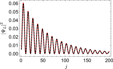
Figure 6: The MF probability density $\left|\Psi_{L}\right|^{2}$ on the site $j$ obtained numerically (red) and analytically (black). Both approaches agree excellently. The tight-binding parameters are chosen to be $N=1000$, $\overline{\alpha}/t_{x}=0.3$, $\Delta/t_{x}=0.005$, $\mu/t_{x}=-0.002$, $V_{Z}/t_{x}=0.01$. We note that such the MF probability density can be measured in STM experiments nadj2014o ; pawlak2016p ; denis .

In a finite-size nanowire of the length $Na$ ($N\ll N^{\prime}$), the two MFs split away from zero energy. This energy splitting can be found perturbatively in the framework of the tight-binding model. Here, we represent the Hamiltonian $\overline{H}$ of the finite chain as $\overline{H}=H_{0}^{L}-H_{1}$, where $H_{0}^{L}$ is the Hamiltonian of the semi-infinite chain and $H_{1}$ is the small perturbation that comes from eliminating the hopping between sites $n=N+1$ and $n=N+2$ and is given by

$$H_{1}=\sum_{\sigma,\sigma^{\prime}}c^{\dagger}_{N+2,\sigma}\Big{[}i\overline{\alpha}(\sigma^{z})_{\sigma\sigma^{\prime}}-t_{x}\delta_{\sigma\sigma^{\prime}}\Big{]}c_{N+1,\sigma^{\prime}}+{\rm H.c.}$$ (14)

As a result, the energy splitting is given by

$$\delta\epsilon=\left|\left\langle 0\left|\gamma_{R}H_{1}\gamma_{L}^{\dagger}\right|0\right\rangle\right|,$$ (15)

where we used the fact that $\mathcal{H}_{0}^{L}\Psi^{L}=0$. In the Bogoliubov-de-Gennes representation, we arrive at

$$\left\langle 0\left|\gamma_{R}H_{1}\gamma_{L}^{\dagger}\right|0\right\rangle=-t_{x}\sum_{\sigma}\Big{[}\left(\chi^{R}_{N+1,1,\sigma}\right)^{*}\chi^{L}_{N+2,1,\sigma}\Big{]}-i\overline{\alpha}\sum_{\sigma}\Big{[}\sigma\left(\chi^{R}_{N+1,1,\sigma}\right)^{*}\chi^{L}_{N+2,1,\sigma}\Big{]}.$$ (16)

This expression can be significantly simplified further by using the properties of the MF wavefunctions: $\chi_{n11}^{L/R}=\left(\chi_{n\bar{1}1}^{L/R}\right)^{*}$ and $\chi_{n1\bar{1}}^{L/R}=\left(\chi_{n\bar{1}\bar{1}}^{L/R}\right)^{*}$. In addition, in our particular setup, $\chi_{n1\bar{1}}^{L}=i\left(\chi_{n11}^{L}\right)^{*}$ and $\chi_{n1\bar{1}}^{R}=-i\left(\chi_{n11}^{R}\right)^{*}$. Thus,

$$\delta\epsilon=2\left|t_{x}{\rm Im}\left[\chi_{N+1,1,1}^{R}\left(\chi_{N+2,1,1}^{L}\right)^{*}\right]-\overline{\alpha}{\rm Re}\left[\chi_{N+1,1,1}^{R}\left(\chi_{N+2,1,1}^{L}\right)^{*}\right]\right|.$$ (17)

To proceed further, we determine $\chi_{N+2,1,1}^{L}$ and $\chi_{N+1,1,1}^{R}$ from the continuum model. Using Eqs. (10) and (11) of the main text, $\chi_{N+2,1,1}^{L}=\sqrt{a}f(x=(N+2)a)/\sqrt{\mathcal{N}}$ and $\chi_{N+1,1,1}^{R}=\sqrt{a}f^{*}(x=a)/\sqrt{\mathcal{N}}$. The normalization prefactor $\mathcal{N}$ is defined from the condition $\int_{0}^{+\infty}dx\ \left|\Psi_{L}(x)\right|^{2}=2$ leading us to

$$\mathcal{N}=\xi^{e}+\xi^{i}-\frac{4\left(1/\xi^{e}+1/\xi^{i}\right)}{(1/\xi^{e}+1/\xi^{i})^{2}+\left(2k_{so}-\mu/\alpha\right)^{2}}.$$ (18)

To simplify the final expression, we introduce the new notation $g=|g|e^{i\varphi}\equiv\chi_{N+1,1,1}^{R}\left(\chi_{N+2,1,1}^{L}\right)^{*}=af^{*}(x=a)f^{*}(x=L)/\mathcal{N}$. In this case, Eq.(17) can be rewritten as

$$\delta\epsilon=2\sqrt{t_{x}^{2}+\overline{\alpha}^{2}}|g|\left|\cos(\varphi+\varphi_{0})\right|,$$ (19)

where $\cos\varphi_{0}=\overline{\alpha}/\sqrt{t_{x}^{2}+\overline{\alpha}^{2}}$. Next, we determine $|g|$ and $\varphi$ by performing a Taylor expansion,

$$g=-\dfrac{ae^{i\varphi_{L}}}{\mathcal{N}}\left(e^{-i\left(2k_{so}-\mu/\alpha\right)a-a/\xi^{e}}-e^{-a/\xi^{i}}\right)\left(e^{-i\left(2k_{so}-\mu/\alpha\right)L-L/\xi^{e}}-e^{-L/\xi^{i}}\right),$$ (20)

$$g\approx\dfrac{a^{2}e^{i\varphi_{L}}}{\mathcal{N}}\left(i\left(2k_{so}-\mu/\alpha\right)+1/\xi^{e}-1/\xi^{i}\right)\left(e^{-i\left(2k_{so}-\mu/\alpha\right)L-L/\xi^{e}}-e^{-L/\xi^{i}}\right),$$ (21)

$$g\approx\dfrac{a^{2}e^{i\left(\varphi_{L}+\theta+\theta^{\prime}\right)}}{\mathcal{N}}\sqrt{\left(1/\xi^{e}-1/\xi^{i}\right)^{2}+\left(2k_{so}-\mu/\alpha\right)^{2}}\sqrt{e^{-2L/\xi^{e}}+e^{-2L/\xi^{i}}-2e^{-L/\xi^{e}}e^{-L/\xi^{i}}\cos\left[\left(2k_{so}-\mu/\alpha\right)L\right]}.$$ (22)

The phase of $g$ is given by $\varphi=\varphi_{L}+\theta+\theta^{\prime}$, where

$$\theta=\arctan\left(\dfrac{2k_{so}-\mu/\alpha}{1/\xi^{e}-1/\xi^{i}}\right),\ \ \theta^{\prime}=\arctan\left(\dfrac{e^{-L/\xi^{e}}\sin\left[\left(2k_{so}-\mu/\alpha\right)L\right]}{e^{-L/\xi^{i}}-e^{-L/\xi^{e}}\cos\left[\left(2k_{so}-\mu/\alpha\right)L\right]}\right).$$ (23)

In the strong SOI regime ($\mathcal{N}\approx\xi^{e}+\xi^{i}$, $\varphi_{0}\approx\pi/2$, $\theta\approx\pi/2$), we arrive at the following expression for the energy splitting between the two MFs,

$$\delta\epsilon\approx 2\frac{\hbar\upsilon_{F}}{\xi^{e}+\xi^{i}}\sqrt{e^{-2L/\xi^{e}}+e^{-2L/\xi^{i}}-2e^{-L/\xi^{e}}e^{-L/\xi^{i}}\cos\left[\left(2k_{so}-\mu/\alpha\right)L\right]}\left|\cos\left(\varphi_{L}+\theta^{\prime}\right)\right|\,,$$ (24)

where $\xi^{i}$ depends non-monotonically on the applied magnetic field. If orbital effects of the magnetic field are taken into account, $\xi^{i}$ first shrinks as a function of magnetic field. However, close to the second topological phase transition, it starts to grow. Next, we analyze Eq. (24) in two regimes: close and far away from the topological phase transition points.

Away from the topological phase transition points, the exterior gap is the smallest in the system, so $\xi^{e}\gg\xi^{i}$. As a result, we arrive at the simplified expression

$$\delta\epsilon\approx 2\Delta e^{-L/\xi^{e}}\left|\cos\left[\varphi_{L}-\left(2k_{so}-\mu/\alpha\right)L\right]\right|.$$ (25)

The amplitude of oscillations, $2\Delta e^{-L/\xi^{e}}$, stays constant as a function of magnetic field. For $\mu=\mu_{0}-\beta V_{Z}^{2}$ the period of oscillations in Zeeman energy is given by $\delta V_{Z}=\pi\alpha/2\beta LV_{Z}$ and stays almost constant if $\delta V_{Z}\ll V_{Z}$. However, there is a tendency for shrinking of the period. It should be contrasted with the regime of weak SOI rainis2013t , where the period of oscillations grows as $\delta V_{Z}=\pi\hbar\sqrt{2V_{Z}/m^{*}}/L$. We note that oscillations in the strong SOI regime arise only due to orbital effects. If we would neglect the shift of the chemical potential caused by the magnetic field via orbital effects, $\mu$ would stay constant as well as the energy splitting $\delta\epsilon$ as a function of the magnetic field.

Close to the phase transition points $\xi^{i}\gg\xi^{e}$ and the energy splitting is given by $\delta\epsilon\approx 2\left(\sqrt{V_{Z}^{2}-\mu^{2}}-\Delta\right)e^{-L/\xi^{i}}\left|\cos\left(\varphi_{L}+\theta^{\prime}\right)\right|$. On one hand, the amplitude of oscillations is enhanced by the exponential prefactor $e^{-L/\xi^{i}}$. On the other hand, the prefactor $1/\xi^{i}$ overtakes the behavior, resulting in the suppression of the splitting as $\xi^{i}$ diverges. Generally, the region of values of the magnetic field, in which $\xi^{i}\gg\xi^{e}$, is very narrow and it is difficult to determine the period of oscillations analytically. However, we observe numerically that the splitting between MFs both decays and oscillates as a function of magnetic field close to the second topological phase transition point, see Fig. 7.

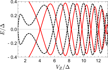
Figure 7: The energy splitting between two MFs as a function of applied magnetic field in units of $V_{Z}/\Delta$ in the finite-size nanowire $L/a=302$. The results were obtained numerically (red solid line) by exact diagonalization of Eq. (12) of the main text and analytically (black dashed line) using Eq. (24), see Fig. 5 of the main text. Generally, there is a reasonable agreement between two approaches. The parameters are fixed as $E_{so}/\Delta=50$ and $\mu=-0.075V_{Z}^{2}/\Delta$.

II Linear dependence of the chemical potential on magnetic field: $\mu=\mu_{0}-\beta_{2}V_{Z}$

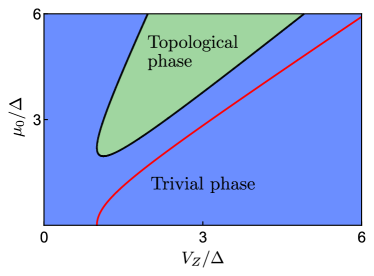
Figure 8: Topological phase diagram as a function of applied magnetic field in units of $V_{Z}/\Delta$ and initial chemical potential $\mu_{0}/\Delta$ in the case of linear shift of chemical potential ($\beta_{2}=2.2$). The topological (green area) and trivial (blue area) phases are separated by the phase boundary (black line) corresponding to the closing of the bulk gap. The red line indicates the phase boundary in the absence of orbital magnetic effects. Again, the topological phase is shifted towards higher values of initial chemical potential.

In this section, we briefly comment on the case if the chemical potential moves linearly as a function of magnetic field. This is the case for degenerate bands and also holds for high values of magnetic fields for all subbands. Thus, we assume that the chemical potential linearly depends on the magnetic field,

$$\mu=\mu_{0}-\beta_{2}V_{Z},$$ (26)

where $\mu_{0}$ is the initial value of the chemical potential and $\beta_{2}$ is the dimensionless parameter, which is chosen to be positive so that $\beta_{2}V_{Z}>0$. For $1<\beta_{2}^{2}<1+\left(\mu_{0}/\Delta\right)^{2}$ the system is in the topological phase if $\mu_{0}>0$ and $V_{Z,-}<V_{Z}<V_{Z,+}$, where the two critical values of magnetic field are defined as

$$V_{Z,\pm}=\dfrac{\beta_{2}\mu_{0}\pm\sqrt{\mu_{0}^{2}+(1-\beta_{2}^{2})\Delta^{2}}}{\beta_{2}^{2}-1}.$$ (27)

In this case, we observe similar oscillations of the energy splitting between two MFs (see Fig. 9). Again, the amplitude stays constant for a large range of magnetic fields, $\xi^{e}\gg\xi^{i}$. Close to the second topological phase transition point $V_{Z,+}$, the amplitude of oscillations shrinks. Generally, this region of shrinking amplitude gets larger due to the slower dependence of $\mu$ on $V_{Z}$. The period of oscillations is constant and is given by $\delta V_{Z}=\pi\alpha/\beta_{2}L$.

If $\beta_{2}^{2}<1$ the system is in the topological phase for $V_{Z}>V_{Z,-}$ and there is no second topological phase transition. In the special case when $\beta_{2}=1$, the system is in the topological phase for $V_{Z}>\left(\Delta^{2}+\mu_{0}^{2}\right)/2\mu_{0}$ and $\mu_{0}>0$.

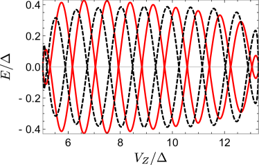
Figure 9: The MF energy splitting as a function of applied magnetic field in units of $V_{Z}/\Delta$ in a finite-size nanowire $k_{so}L=151$. The results were obtained numerically (red solid line) by exact diagonalization of Eq. (12) of the main text and analytically (black dashed line) using Eq. (24). The parameters are chosen as $E_{so}/\Delta=50$ and the chemical potential $\mu/\Delta=16-2.2V_{Z}/\Delta$ is assumed to be linearly shifted due to orbital magnetic effects.

III Dependence of proximity-induced superconducting gap on magnetic field

Next, we also include effects of the external magnetic field on the bulk $s$-wave superconductor in the regime of strong coupling between nanowire and bulk superconductor reeg2017f . The proximity-induced gap $\Delta=\Delta_{0}\sqrt{1-\left(V_{Z}/V_{Z}^{c}\right)^{2}}$ is suppressed at the critical field $V_{Z}^{c}$, where $\Delta_{0}$ is the value of the superconducting gap in the absence of magnetic fields. We note that in the weak coupling regime, the proximity induced gap is determined by the tunneling rate between the nanowire and the bulk superconductor and, thus, the proximity-induced gap in the nanowire can be considered independent of the external magnetic field acting on the bulk superconductor sau2010r ; potter2011e ; kopnin2011p ; zyuzin2013c ; takane2013s ; van2016c ; reeg2017d .

III.1 Constant chemical potential $\mu=\mu_{0}$

If the bottom of the band is not shifted by orbital effects due to the magnetic field, the chemical potential stays constant $\mu=\mu_{0}$. The topological criterion is only slightly modified to

$$\sqrt{\dfrac{\mu_{0}^{2}+\Delta_{0}^{2}}{1+\left(\Delta_{0}/V_{Z}^{c}\right)^{2}}}<V_{Z}<V_{Z}^{c}\,.$$ (28)

In this case, there are no oscillations in the energy splitting [see Fig. 10(a)] since the oscillations could only appear due to the shift of the chemical potential with magnetic field. As a result, the amplitude of the energy splitting, first, rapidly increases and subsequently stays almost constant up to the point where the proximity-induced gap closes at $V_{Z}=V_{Z}^{c}$.

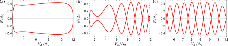
Figure 10: The energy splitting between two MFs as a function of applied magnetic field in units of $V_{Z}/\Delta_{0}$ in a finite-size nanowire $k_{so}L=151$ with $E_{so}/\Delta_{0}=50$. The parameters of the superconducting gap are chosen as follows $\Delta=\Delta_{0}\sqrt{1-\left(V_{Z}/V_{Z}^{c}\right)^{2}}$ with $V_{Z}^{c}=12\Delta_{0}$, where $V_{Z}^{c}$ corresponds to the critical magnetic field $B^{c}=2$ T for $\Delta_{0}=0.25$ meV. (a) The chemical potential is fixed to $\mu_{0}/\Delta_{0}=2$. As expected, if the chemical potential is kept constant, there are no oscillations in the energy splitting. (b) The chemical potential is shifted quadratically due to orbital effects as $\mu/\Delta_{0}=-0.075V_{z}^{2}/\Delta_{0}^{2}$. (c) The chemical potential is shifted linearly due to orbital effects as $\mu/\Delta_{0}=16-2.2V_{z}/\Delta_{0}$. We note that in both panels (b) and (c), there are oscillations in the energy splitting between MFs and there is a range of magnetic fields for which the MF energy splitting amplitude stays almost constant.

III.2 Quadratic dependence of the chemical potential $\mu=\mu_{0}-\beta V_{Z}^{2}$

Now we consider the chemical potential that is shifted as a quadratic function of magnetic field via orbital effects, $\mu=\mu_{0}-\beta V_{Z}^{2}$. If $\mu_{0}>-\left(1+\left(\Delta_{0}/V_{Z}^{c}\right)^{2}\right)/2\beta$ and $\mu_{0}>\left[4\beta^{2}\Delta_{0}^{2}-\left(1+\left(\Delta_{0}/V_{Z}^{c}\right)^{2}\right)^{2}\right]/\left[4\beta\left(1+\left(\Delta_{0}/V_{Z}^{c}\right)^{2}\right)\right]$ the system is in the topological phase for $V_{Z,-}<V_{Z}<\text{min}\{V_{Z,+},V_{Z}^{c}\}$, where

$$V_{Z,\pm}=\sqrt{\dfrac{\left(1+2\beta\mu_{0}+(\Delta_{0}/V_{Z}^{c})^{2}\right)\pm\sqrt{\left(1+2\beta\mu_{0}+(\Delta_{0}/V_{Z}^{c})^{2}\right)^{2}-4\beta^{2}(\Delta_{0}^{2}+\mu_{0}^{2})}}{2\beta^{2}}}.$$ (29)

Again, in the strong coupling regime, the proximity-induced gap $\Delta=\Delta_{0}\sqrt{1-\left(V_{Z}/V_{Z}^{c}\right)^{2}}$ decreases as the magnetic field is increased. Thus, the localization length $\xi^{e}$, which now depends on $V_{Z}$, increases with increasing the magnetic field. Away from the topological phase transition point $V_{Z,-}$, the localization length $\xi^{e}\gg\xi^{i}$ and the energy splitting first increases with increasing $V_{Z}$ and then starts to decrease (there is an interplay between the growing prefactor $e^{-L/\xi^{e}}$ and the decreasing one $\Delta$), see Fig. 10(b). Close to the topological phase transition point $V_{Z,-}$, the localization length $\xi^{i}\gg\xi^{e}$, so the energy splitting is increasing in this very narrow region.

III.3 Linear dependence of the chemical potential $\mu=\mu_{0}-\beta_{2}V_{Z}$

Finally, we consider the chemical potential that linearly depends on the magnetic field, $\mu=\mu_{0}-\beta_{2}V_{Z}$. For $1+(\Delta_{0}/V_{Z}^{c})^{2}<\beta_{2}^{2}<\left(1+(\mu_{0}/\Delta_{0})^{2}\right)\left(1+(\Delta_{0}/V_{Z}^{c})^{2}\right)$ the system is in the topological phase if $\mu_{0}>0$ and $V_{Z,-}<V_{Z}<\text{min}\{V_{Z,+},V_{Z}^{c}\}$, where

$$V_{Z,\pm}=\dfrac{\beta_{2}\mu_{0}\pm\sqrt{\beta_{2}^{2}\mu_{0}^{2}+(\Delta_{0}^{2}+\mu_{0}^{2})\left(-\beta_{2}^{2}+1+(\Delta_{0}/V_{Z}^{c})^{2}\right)}}{\left(\beta_{2}^{2}-1-(\Delta_{0}/V_{Z}^{c})^{2}\right)}.$$ (30)

In this case, we observe oscillations of the energy splitting that have similar features as the ones obtained for the quadratic dependence of the chemical potential [see Fig. 10(c)]. For $\beta_{2}^{2}<1+(\Delta_{0}/V_{Z}^{c})^{2}$ the system is in the topological phase if $V_{Z,-}<V_{Z}<V_{Z}^{c}$. In the special case $\beta_{2}^{2}=1+(\Delta_{0}/V_{Z}^{c})^{2}$, the system is in the topological phase if $\mu_{0}>0$ and $\left(\Delta_{0}^{2}+\mu_{0}^{2}\right)/2\mu_{0}\sqrt{1+(\Delta_{0}/V_{Z}^{c})^{2}}<V_{Z}<V_{Z}^{c}$.

References

- (1) J. Alicea, Phys. Rev. B 81, 125318 (2010).
- (2) R. M. Lutchyn, J. D. Sau, and S. Das Sarma, Phys. Rev. Lett. 105, 077001 (2010).
- (3) Y. Oreg, G. Refael, and F. von Oppen, Phys. Rev. Lett. 105, 177002 (2010).
- (4) S. Gangadharaiah, B. Braunecker, P. Simon, and D. Loss, Phys. Rev. Lett. 107, 036801 (2011).
- (5) D. Sticlet, C. Bena, and P. Simon, Phys. Rev. Lett. 108, 096802 (2012).
- (6) F. Domínguez, F. Hassler, and G. Platero, Phys. Rev. B 86, 140503(R) (2012).
- (7) E. Prada, P. San-Jose, and R. Aguado, Phys. Rev. B 86, 180503(R) (2012).
- (8) D. Rainis, L. Trifunovic, J. Klinovaja, and D. Loss, Phys. Rev. B 87, 024515 (2013).
- (9) F. Maier, J. Klinovaja, and D. Loss, Phys. Rev. B 90, 195421 (2014).
- (10) S. Das Sarma, J. D. Sau, and T. D. Stanescu, Phys. Rev. B 86, 220506 (2012).
- (11) M. Leijnse and K. Flensberg, Semicond. Sci. Technol. 27, 124003 (2012).
- (12) J. Klinovaja, P. Stano, and D. Loss, Phys. Rev. Lett. 109, 236801 (2012).
- (13) K. Björnson and A. M. Black-Schaffer, Phys. Rev. B 88, 024501 (2013).
- (14) L. Weithofer, P. Recher, and T. L. Schmidt, Phys. Rev. B 90, 205416 (2014).
- (15) O. Dmytruk, M. Trif, and P. Simon, Phys. Rev. B 92, 245432 (2015).
- (16) S. Nakosai, J. C. Budich, Y. Tanaka, B. Trauzettel, and N. Nagaosa, Phys. Rev. Lett. 110, 117002 (2013).
- (17) C. R. Reeg and D. L. Maslov, Phys. Rev. B 90, 024502 (2014).
- (18) P. W. Brouwer, M. Duckheim, A. Romito, and F. von Oppen, Phys. Rev. Lett. 107, 196804 (2011).
- (19) W. DeGottardi, M. Thakurathi, S. Vishveshwara, and D. Sen, Phys. Rev. B 88, 165111 (2013).
- (20) M. Thakurathi, O. Deb, and D. Sen, J. Phys. Condens. Matter 27, 275702 (2015).
- (21) B. Scharf and I. Žutić, Phys. Rev. B 91, 144505 (2015).
- (22) J. Klinovaja, S. Gangadharaiah, and D. Loss, Phys. Rev. Lett. 108, 196804 (2012).
- (23) J. Klinovaja, G. J. Ferreira, and D. Loss, Phys. Rev. B 86, 235416 (2012).
- (24) J. Klinovaja and D. Loss, Phys. Rev. X 3, 011008 (2013).
- (25) C. Dutreix, M. Guigou, D. Chevallier, and C. Bena, Eur. Phys. J. B 87, 296 (2014).
- (26) J. Klinovaja and D. Loss, Phys. Rev. B 88, 075404 (2013).
- (27) A. M. Black-Schaffer, Phys. Rev. Lett. 109, 197001 (2012).
- (28) P. San-Jose, J. L. Lado, R. Aguado, F. Guinea and J. Fernández-Rossier, Phys. Rev. X 5, 041042 (2015).
- (29) B. T. Zhou, N. F. Q. Yuan, H.-L. Jiang,and K. T. Law, Phys. Rev. B 93, 180501(R) (2016).
- (30) V. Kaladzhyan and C. Bena, SciPost Phys. 3, 002 (2017)
- (31) S. Nadj-Perge, I. K. Drozdov, B. A. Bernevig, and A. Yazdani, Phys. Rev. B 88, 020407 (2013).
- (32) J. Klinovaja, P. Stano, A. Yazdani, and D. Loss, Phys. Rev. Lett. 111, 186805 (2013).
- (33) B. Braunecker and P. Simon, Phys. Rev. Lett. 111, 147202 (2013).
- (34) M. M. Vazifeh and M. Franz, Phys. Rev. Lett. 111, 206802 (2013).
- (35) F. Pientka, L. I. Glazman, and F. von Oppen, Phys. Rev. B 88, 155420 (2013).
- (36) K. Pöyhönen, A. Westström, J. Röntynen, and T. Ojanen, Phys. Rev. B 89, 115109 (2014).
- (37) V. Mourik, K. Zuo, S. M. Frolov, S. R. Plissard, E. P. A. M. Bakkers, and L. P. Kouwenhoven, Science 336, 1003 (2012).
- (38) A. Das, Y. Ronen, Y. Most, Y. Oreg, M. Heiblum, and H. Shtrikman, Nat. Phys. 8, 887 (2012).
- (39) M. Deng, C. Yu, G. Huang, M. Larsson, P. Caroff, and H. Xu, Nano Lett. 12, 6414 (2012).
- (40) H. O. H. Churchill, V. Fatemi, K. Grove-Rasmussen, M. T. Deng, P. Caroff, H. Q. Xu, and C. M. Marcus, Phys. Rev. B 87, 241401(R) (2013).
- (41) S. M. Albrecht, A. P. Higginbotham, M. Madsen, F. Kuemmeth, T. S. Jespersen, J. Nygård, P. Krogstrup, and C. M. Marcus, Nature 531, 206 (2016).
- (42) S. Nadj-Perge, I. K. Drozdov, J. Li, H. Chen, S. Jeon, J. Seo, A. H. MacDonald, B. A. Bernevig, and A. Yazdani, Science 346, 602 (2014).
- (43) M. Ruby, F. Pientka, Y. Peng, F. von Oppen, B. W. Heinrich, and K. J. Franke, Phys. Rev. Lett. 115, 197204 (2015).
- (44) R. Pawlak, M. Kisiel, J. Klinovaja, T. Meier, S. Kawai, T. Glatzel, D. Loss, and E. Meyer, npj Quantum Inf. 2, 16035 (2016).
- (45) L. P. Rokhinson, X. Liu, and J. K. Furdyna, Nat. Phys. 8,795 (2012).
- (46) J. C. Estrada Saldaña, J. P. Cleuziou, E. J. H. Lee, D. Car, S. R. Plissard, E. P. A. M. Bakkers, and S. De Franceschi, arXiv:1709.02614.
- (47) C. X. Liu, F. Setiawan, J. D. Sau, and S. Das Sarma, Phys. Rev. B 96, 054520 (2017).
- (48) J. S. Lim, R. Lopez, and L. Serra, Europhys. Lett. 103, 37004 (2013).
- (49) B. Nijholt and A. R. Akhmerov, Phys. Rev. B 93, 235434 (2016).
- (50) C. Fasth, A. Fuhrer, L. Samuelson, V. N. Golovach, and D. Loss, Phys. Rev. Lett. 98, 266801 (2007).
- (51) S. Nadj-Perge, V. S. Pribiag, J. W. G. van den Berg, K. Zuo, S. R. Plissard, E. P. A. M. Bakkers, S. M. Frolov, and L. P. Kouwenhoven, Phys. Rev. Lett. 108, 166801 (2012).
- (52) I. van Weperen, B. Tarasinski, D. Eeltink, V. S. Pribiag, S. R. Plissard, E. P. A. M. Bakkers, L. P. Kouwenhoven, and M. Wimmer, Phys. Rev. B 91, 201413(R) (2015).
- (53) J. Kammhuber, M. C. Cassidy, F. Pei, M. P. Nowak, A. Vuik, Ö. Gül, D. Car, S. R. Plissard, E. P. A. M. Bakkers, M. Wimmer, and L. P. Kouwenhoven, Nature Communications 8, 478 (2017).
- (54) G. W. Winkler, D. Varjas, R. Skolasinski, A. A. Soluyanov, M. Troyer, and M. Wimmer, arXiv:1703.10091.
- (55) F. Geerinckx, F. Peeters, and J. Devreese, J. Appl. Phys. 68, 3435 (1990).
- (56) A. V. Madhav and T. Chakraborty, Phys. Rev. B 49, 8163 (1994).
- (57) G. Burkard, D. Loss, and D. P. DiVincenzo, Phys. Rev. B 59, 2070 (1999).
- (58) E. Tsitsishvili, G. S. Lozano, and A. O. Gogolin, Phys. Rev. B 70, 115316 (2004).
- (59) B. Braunecker, G. I. Japaridze, J. Klinovaja, and D. Loss, Phys. Rev. B 82, 045127 (2010).
- (60) J. Klinovaja and D. Loss, Phys. Rev. B 86, 085408 (2012).
- (61) J. Klinovaja and D. Loss, Eur. Phys. J. B 88, 62 (2015).
- (62) See the Supplemental Material at for detailed derivation of the energy splitting between MFs and for case of linear dependence of the chemical potential on applied magnetic field, in which we also take into account the suppression of the bulk superconducting gap.
- (63) J. D. Sau, R. M. Lutchyn, S. Tewari, and S. Das Sarma, Phys. Rev. B 82, 094522 (2010).
- (64) A. C. Potter and P. A. Lee, Phys. Rev. B 83, 184520 (2011).
- (65) N. B. Kopnin and A. S. Melnikov, Phys. Rev. B 84, 064524 (2011).
- (66) A. A. Zyuzin, D. Rainis, J. Klinovaja, and D. Loss, Phys. Rev. Lett. 111, 056802 (2013).
- (67) Y. Takane and R. Ando, J. Phys. Soc. Jpn. 83, 014706 (2014).
- (68) B. van Heck, R. M. Lutchyn, and L. I. Glazman, Phys. Rev. B 93, 235431 (2016).
- (69) C. Reeg, J. Klinovaja, and D. Loss, Phys. Rev. B 96, 081301(R) (2017).
- (70) C. Reeg, D. Loss, and J. Klinovaja, Phys. Rev. B 96, 125426 (2017).

References

- (1) J. Klinovaja and D. Loss, Phys. Rev. B 86, 085408 (2012).
- (2) J. Klinovaja, P. Stano, and D. Loss, Phys. Rev. Lett. 109, 236801 (2012).
- (3) S. Nadj-Perge, I. K. Drozdov, J. Li, H. Chen, S. Jeon, J. Seo, A. H. MacDonald, B. A. Bernevig, and A. Yazdani, Science 346, 602 (2014).
- (4) R. Pawlak, M. Kisiel, J. Klinovaja, T. Meier, S. Kawai, T. Glatzel, D. Loss, and E. Meyer, npj Quantum Inf. 2, 16035 (2016).
- (5) D. Chevallier and J. Klinovaja, Phys. Rev. B 94, 035417 (2016).
- (6) D. Rainis, L. Trifunovic, J. Klinovaja, and D. Loss, Phys. Rev. B 87, 024515 (2013).
- (7) C. Reeg, D. Loss, and J. Klinovaja, Phys. Rev. B 96, 125426 (2017).
- (8) J. D. Sau, R. M. Lutchyn, S. Tewari, and S. Das Sarma, Phys. Rev. B 82, 094522 (2010).
- (9) A. C. Potter and P. A. Lee, Phys. Rev. B 83, 184520 (2011).
- (10) N. B. Kopnin and A. S. Melnikov, Phys. Rev. B 84, 064524 (2011).
- (11) A. A. Zyuzin, D. Rainis, J. Klinovaja, and D. Loss, Phys. Rev. Lett. 111, 056802 (2013).
- (12) Y. Takane and R. Ando, J. Phys. Soc. Jpn. 83, 014706 (2014).
- (13) B. van Heck, R. M. Lutchyn, and L. I. Glazman, Phys. Rev. B 93, 235431 (2016).
- (14) C. Reeg, J. Klinovaja, and D. Loss, Phys. Rev. B 96, 081301(R) (2017).