Estimating the number of casualties in the American Indian war: a Bayesian analysis using the power law distribution

Abstract

The American Indian war lasted over one hundred years, and is a major event in the history of North America. As expected, since the war commenced in late eighteenth century, casualty records surrounding this conflict contain numerous sources of error, such as rounding and counting. Additionally, while major battles such as the Battle of the Little Bighorn were recorded, many smaller skirmishes were completely omitted from the records. Over the last few decades, it has been observed that the number of casualties in major conflicts follows a power law distribution. This paper places this observation within the Bayesian paradigm, enabling modelling of different error sources, allowing inferences to be made about the overall casualty numbers in the American Indian war.

math.PR/0000000

1 Introduction

The American Indian war spanned the time period, 1778 to around 1890, and covered a wide geographical area. As such, the participants, and to a certain extent, technology changed throughout the war. Although some authors have attempted to divide the period into separate conflicts (see, for example, Clodfelter (2008) and Axelrod (1993)), there is no agreed time period division. This time was characterised by low-level violence with occasional large scale battles, such as, the 1794 Battle of Fallen Timbers, 1811 Battle of Tippecanoe. and 1876 the battle of the little Bighorn.

Around the time of American independence ($\sim\!\!1780$) the majority of the population lived near the sea and the country had a limited military capacity. Consequently most of the casualties were due to small skirmishes which occasionally led to larger conflicts.

During the early nineteenth century, many tribes were relocated to lands west of the Mississippi river. Most removals were met with relatively little violence, but in a few cases, tribes fought long conflicts to stay on their land. The relocations carried on throughout the nineteenth century, with native Americans being increasingly confined to reservations.

It has been observed that the severity of many violent events follow a power law distribution. In a seminal paper, Richardson (1948) divided international and domestic instances of violence between $1820$ and $1945$ into logarithmic groups. A subsequent paper (Richardson, 1960), with an updated data set, demonstrated that the frequency of entries in each logarithmic group, followed a simple multiplicative law: for each $10$–fold increase in the number of casualties, the frequency decreased by around a factor of three. Cederman (2003) updated this analysis with data (restricted to interstate wars) from the Correlates of War (COW) Project (Geller and Singer, 1998). Cederman found that the multiplicative law seemed to hold for the last two centuries. He then developed agent-based models to suggest possible generative mechanisms for this “law”.

Clauset, Young and Gleditsch (2007) extended this work to include terrorist attacks since 1968. They noted that the frequency-severity statistics of terrorist events are scale invariant and concluded that there is no fundamental difference between small and large attacks. Similarly, Bohorquez et al. (2009) investigated the severity of insurgent attacks within nine separate conflicts and again found that the data had a power law structure.

Power law distributions are often described as “scale-free”, indicating that common small events are qualitatively similar to large rare events. If this pattern can be detected in empirical data, it may indicate the presence of an interesting underlying process. Being able to detect whether a system does or does not follow a power law can provide hints to the generative mechanisms at work. During the twentieth century, numerous examples of these heavy tailed distributions have been used to describe a variety of different phenomena, including city size, word frequency and the productivity of scientists; see, for example Newman (2005), Dewez et al. (2013) and Bell et al. (2012).

This apparent ubiquity of power laws in a wide range of disciplines was questioned by Stumpf and Porter (2012). The authors pointed out that many “observed” power law relationships are highly suspect. In particular, estimating the power law exponent from a log-log plot, whilst simple and appealing, is a very poor technique for fitting these types of models. Instead, a systematic, principled and statistically rigorous approach should be applied, such as those by Clauset, Shalizi and Newman (2009), Breiman, Stone and Kooperberg (1990), Dekkers and Dehaan (1993), and Drees and Kaufmann (1998).

The common problem with fitting the power law distribution is that analyses typically assume that the power law phenomena is present in the tail of the distribution. This results in the need to estimate both the scaling parameter $\alpha$ and the lower bound threshold for where the power law behaviour begins, $x_{\min}$. Clauset, Shalizi and Newman (2009) (CSN) introduced a principled set of methods for fitting and testing power law distributions. Their approach is straightforward and couples a distance-based test for estimating $x_{\min}$ with estimation of $\alpha$ via maximum likelihood. Alternative models, such as the log normal distribution, can be compared using a likelihood ratio test (Vuong, 1989). However this method does have a few issues. First, after estimating $x_{\min}$, we discard all data below this threshold. Second, it is unclear how to compare distributions with different $x_{\min}$ values. Third, although it is possible to make predictions in the tail of the distribution, making future predictions over the entire data space is not possible since values less than $x_{\min}$ have not been directly modelled (Clauset and Woodard, 2013).

One further difficulty with the method proposed by CSN is that it is not straightforward to incorporate an error model during the inference stage. Recently, Virkar and Clauset (2014) considered a model for binned data in which the observed data has been rounded or grouped. Essentially, the authors propose a modification to the CSN algorithm. However, this modification is difficult to generalise to other error structures and also suffers from the same issues as the original method.

In this paper we use a power law distribution to model the number of casualties sustained in the American Indian war. By adopting a Bayesian approach we are able to model the under-reporting of casualties, incorporate prior beliefs on the parameters and provide predictions for the true number of casualties. In the following section, we discuss the power law distribution and the CSN method in more detail. In section 3, we give a brief introduction to the American Indian war, before moving on to a fully Bayesian analysis of the model. The paper closes with a discussion in section 4.

2 The power law distribution

The discrete power law distribution has the probability mass function (PMF)

$$\text{Pr}(X=x)=\frac{x^{-\alpha}}{\zeta(\alpha,x_{\min})},\quad x=x_{\min},x_{\min}+1,\ldots$$ (1)

where

$$\zeta(\alpha,x_{\min})=\sum_{n=0}^{\infty}(n+x_{\min})^{-\alpha}$$ (2)

is the generalized zeta function which converges provided $\alpha>1$ (Abramowitz and Stegun, 1970). When $x_{\min}=1$, $\zeta(\alpha,1)$ simplifies to the standard zeta function, $\zeta(\alpha)=\sum_{n=1}^{\infty}n^{-\alpha}.$

The value of $\alpha$ determines which moments diverge. For example, if $1<\alpha\leq 2$, all moments diverge, i.e., $E[X^{m}]=\infty$, $m=1,\ldots$; if $2<\alpha\leq 3$, all second and higher-order moments diverge, i.e., $E[X^{m}]=\infty$, $m=2,\ldots$; and so on.

2.1 Parameter inference

Clauset, Shalizi and Newman (2009) show that when $x_{\min}$ is known, an approximate maximum likelihood estimate for the discrete power law scaling parameter $\alpha$ is

$$\hat{\alpha}\simeq 1+n\left[\sum_{i=1}^{n}\ln\left(\frac{x_{i}}{x_{\min}-0.5}\right)\right]^{-1}\;.$$ (3)

The likelihood estimate for the continuous power law is almost identical, but with the $0.5$ removed from the denominator. In many practical situations, it is argued that only the tail of the distribution follows a power law, but the value of $x_{\min}$ is unknown. Unfortunately, as the value of $x_{\min}$ increases, the amount of data that is discarded also increases, so it is clear that some care must be taken when estimating this parameter. Estimation via maximum likelihood is not appropriate since for each value of $x_{\min}$, the likelihood function is calculated using a different data set.

Until recently, a common approach used to estimate $x_{\min}$ has been from a visual inspection of the data on a log-log plot. Clearly, this is error prone and subjective (Stumpf and Porter, 2012). The de-facto method for estimating the lower bound $x_{\min}$ and corresponding scaling parameter $\alpha$ is the Kolmogorov-Smirnov technique proposed by Clauset, Shalizi and Newman (2009). Denoting $F(x)$ and $\hat{F}(x)$ to be the CDFs of the model and data respectively (for $x\geq x_{\min}$), the lower bound $x_{\min}$ can be estimated by minimising the statistic

$$D=\max_{x\geq x_{\min}}|F(x)-\hat{F}(x)|\;.$$ (4)

For a given value of $x_{\min}$, the MLE standard error of $\alpha$ can be derived analytically. However, this ignores the additional uncertainty due to the lower bound estimate, $x_{\min}$. To quantify uncertainty a bootstrap procedure can be used (Efron and Tibshirani, 1993). Essentially, we sample with replacement from the original data set and then re-infer the parameters at each step using Algorithm 1.

Algorithm 1 Estimating the uncertainty in $x_{\min}$ (Clauset, Young and Gleditsch, 2007)

1:	Set $N$ equal to the number of values in the original data set.
2:	for i in 1:B:
3:	Sample $N$ values (with replacement) from the original data set.
4:	Estimate $x_{\min}$ and $\alpha$ by minimising the Kolmogorov-Smirnov statistic.
5:	end for

To test whether the data set of interest follows a power law, we can employ another bootstrapping procedure. Essentially, for each bootstrap we simulate a new data set using the inferred parameters and refit the model. However, this can be computationally prohibitive.

The Kolmogorov-Smirnoff procedure developed by CSN is principled, relatively straightforward to apply and is a substantial improvement over estimating the parameters by eye. Consequently it is widely used and has been implemented in both python (Alstott, Bullmore and Plenz, 2014) and R (Gillespie, 2015) programming languages.

Many data sets are collected with error. Thus even if $X$ follows a power law, we typically observe a corrupted version. For example, in Virkar and Clauset (2014), the authors extend the CSN method to fit binned data, that is, within a set of $k$ boundaries, $0<b_{1}<b_{2}<\ldots<b_{k}$, we only observe the number of observations that fall within a particular region. So as $k\rightarrow\infty$, we fully observe the process. Again the difficulty with the estimation process is that we are only modelling the tail of the distribution and so need to infer the cut-off $x_{\min}$. Extending this framework to deal with more complex error models is non-trivial. For example, in this paper we study the American-Indian data set where we observe $X$ with probability $p$ and a binned value with probability $1-p$, i.e. a proportion of the data has been binned/rounded.

3 Modelling casualties in the American Indian war

This paper builds on Friedman (2015), by attempting to infer the number of casualties that occurred during the American Indian war. Figure 1a shows the casualties sustained by both sides. Small scale conflicts are prominent for both sides during the war. For example, in over 50% of the US American conflicts there were only one or two recorded casualties. For the Native Americans, this proportion was around 25%. Figure 1b gives the $1-$ the empirical CDFs of the data set, where each point represents a specific battle. For power law distributions, the points lie on a straight line. Clearly, for both combatants the points only lie on a line in the tail of the distribution.

Unsurprisingly it is extremely unlikely that data collection alone can give us a precise estimate of the number of casualties sustained by both sides from historical conflicts. The primary issue with the data set is under reporting, particularly with the native American casualties. A secondary issue is data quality. In addition to the usual mis-counting in both the native and US records, there are clear rounding effects in the data.

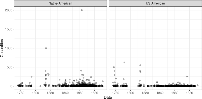
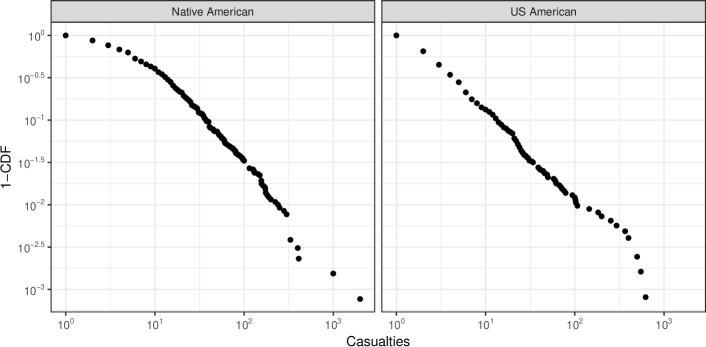
Figure 1: Casualities sustained by the Native American and US American sides during the American Indian war, 1776–1890. Each point represents a particular conflict. Data originally collected and analysed by Friedman (2015). (b) Empirical CDFs of the casualty data set.

3.1 The underlying process

A casualty is defined as a person captured, mortally wounded, or killed in a particular battle or skirmish. Casualties include military engagements that occurred within the continental United States and also any pursuits into neighbouring territories.

In our study of the American Indian war, we assume that the generative mechanism for the numbers of casualties in a particular battle or skirmish for the Native Americans follows a power law distribution, resulting in a likelihood contribution

$$\text{Pr}(W_{i,N}=w_{i,N})=\frac{w_{i,N}^{-\alpha_{N}}}{\zeta(\alpha_{N})}\quad i=1,\ldots,n_{true,N}$$ (5)

where $\zeta(\cdot)$ is the standard zeta function, $w_{i,N}$ is the true number of casualties sustained by the Native Americans in battle/skirmish $i$, and $n_{true,N}$ is the true number of battles/skirmishes for the Native Americans. Note that the total number of casualties sustained by the Native Americans is given by $\sum_{i=1}^{n_{true,N}}w_{i,N}$. Similarly for the US forces we have

$$\text{Pr}(W_{i,U}=w_{i,U})=\frac{w_{i,U}^{-\alpha_{U}}}{\zeta(\alpha_{U})}\quad i=1,\ldots,n_{true,U}\;.$$

Ideally we would have joint records for the casualties sustained by US and Native American forces for each battle. This would enable us to jointly model the number of casualties for each side. Unfortunately the data do not contain this information since battles are missing and casualties are recorded (if at all) after the event. Instead we link the forces by having an informative joint prior on $(\alpha_{N},\alpha_{U})$; this is discussed in more detail in section 3.2.

To make the notation clearer in the following discussion, we will drop the subscripts $N$ and $U$ from the random variables and parameters.

The idea that the number of casualties occurring in a battle comes from a distribution where the variance and/or mean are infinite is not plausible: for any given conflict there is maximum number of casualties that can be sustained. However, it does provide a mechanism for characterising the underlying distribution; this assumption is investigated in section 3.5.

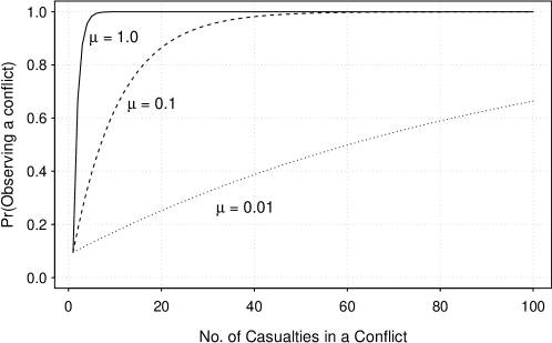
Figure 2: The probability of observing an event for $\lambda=0.1$ and $\mu$ as indicated. The probability of observing an event where there is a single casualty, is $1-e^{-0.1}\simeq 0.1$.

Clearly historical records are not perfect and some conflicts will be omitted. However, battles are not missing at random. Instead conflicts that sustain only a small number of casualties are more likely to be omitted than large scale conflicts. For example, it is unlikely there was a conflict where US forces sustained over $100$ casualties that wasn’t recorded. To model the probability that a conflict was omitted we use a logistic-type function, with $i=1,\ldots,n_{true}$,

$$\text{Pr}(X_{i}=w_{i}|W_{i}=w_{i})=1-\exp\{-\lambda-\mu(w_{i}-1)\}\quad\lambda,\mu>0$$ (6)

otherwise $X_{i}$ is missing. The number of events that we observe is $n_{obs}$. As the number of casualties, $w_{i}$ increases, the probability of observing and recording a conflict, tends to one. Furthermore, the probability of observing a conflict of size $w_{i}=1$ is $1-e^{-\lambda}\simeq\lambda$. A plot of the missingness probability function (6) is shown in Figure 2 for different values of $\mu$, with $\lambda=0.1$. As $\mu$ increases, the probability of observing an event also increases.

Data quality

So far we have assumed that the underlying generative model is a power law, with the probability of observing a battle following expression (6). However even when a battle has been recorded, it is likely that the record contains errors.

The first recording error we consider is a counting error. Since the size of the error is likely to increase with the number of casualties, we will model this error using a Poisson distribution as with this distribution, the variance equals the mean. However, since missing observations are already captured using expression (6), we use a truncated Poisson distribution. Letting $Y_{i}$ to be a noisy measurement of the true number of casualties in observed conflict $i$, we have

$$\text{Pr}(Y_{i}=y_{i}|X_{i}=x_{i})=\frac{x_{i}^{y_{i}}e^{-x_{i}}}{y_{i}!(1-e^{-x_{i}})},\quad y_{i}=1,2,\ldots,i=1,2,\ldots,n_{obs}.$$ (7)

Table 1: Observed number of casualties for the US and Native American forces, e.g. there were $430$ conflicts where the number of US casualties was $1$. The data indicates that rounding to the nearest $5$ casualties has occurred.

	No. of Casualities
	$1$	$2$	$3$	$4$	$5$	$6$	$7$	$8$	$9$	$10$
US	$430$	$247$	$132$	$78$	$\mathbf{\phantom{0}83}$	$45$	$22$	$21$	$10$	$\mathbf{10}$
Native	$166$	$139$	$107$	$69$	$\mathbf{126}$	$51$	$48$	$34$	$31$	$\mathbf{49}$

A further source of error that is present is rounding or heaping (Crawford, Weiss and Suchard, 2015). From Table 1 there is clear evidence that the number casualties have been rounded to the nearest five: for the Native American’s there were $69$ and $51$ events where the number of casualties was $4$ and $6$ respectively, whereas there were $126$ recorded conflicts where the number of casualties was $5$. As might be expected, rounding seems to more prevalent for the Native American casualty figures. For each battle, $i=1,\ldots,n_{obs}$, we assume that no rounding occurs when $y_{i}=1$ or $2$. For values of $y_{i}>2$, the rounding mechanism is modelled as

$$\text{Pr}(Z_{i}=z_{i}|Y_{i}=y_{i})=\begin{cases}y_{i}&\mbox{with probability }1-p\\ 5\times\left(\left[\frac{y_{i}-2.5}{5}\right]+1\right)&\mbox{with probability }p,\end{cases}$$ (8)

where $[\cdot]$ denotes the integer part.

A summary of the modelling process is given in Table 2.

Table 2: A summary of the different modelling stages. The formal definitions are given at the indicated equation numbers.

Variable	Description	Definition
$W_{i}$	The true number of casualties that occurred in conflict $i$.	(5)
$X_{i}$	Was the conflict recorded.	(6)
$Y_{i}$	The number of casualties in a recorded conflict $i$, with Poisson counting errors.	(7)
$Z_{i}$	The observed historical value. The number of casualties in a recorded conflict $i$, with Poisson counting and rounding/heaping errors.	(8)
$n_{obs}$	The total number of observed conflicts.
$n_{true}$	The total of number of conflicts (including missing battles).

3.2 Bayesian parameter estimation

The inference task is two-fold. First, we wish to make statistically valid statements about the unknown model parameters $(\alpha,\lambda,\mu,p)$. Second, we wish to predict the true, unobserved, number of casualties sustained by each force during the conflict. The Bayesian statistical inference approach combines information from the data with prior parameter information. The resulting posterior distribution enables us to make predictions about the actual casualty rates.

We denote $\theta=(\alpha_{U},\lambda_{U},\mu_{U},p_{U},\alpha_{N},\lambda_{N},\mu_{N},p_{N})$ to be the model parameters of both datasets and $z$ to be the combined datasets, $z=(z_{U},z_{N})$ where the subscripts $U$ and $N$ denote the US and Native American forces, respectively.

Prior distributions for the observation rates were obtained from the following:

• A reasonable lower bound for observing a conflict of size $1$, is to only observe $1$ in every one thousand battles, i.e. $1-e^{-\lambda}\simeq 0.001$.

• It is unlikely that we would record all conflicts of size $1$. Instead, we would expect to observe at most $95$% of such events.

• Casualties for the US forces were more likely to be recorded than the Native American forces.

• It is unlikely that large scale conflicts were omitted.

This prior information is captured using a fairly weak bivariate log normal prior, namely

$$\left(\begin{matrix}\lambda_{U}\\ \lambda_{N}\end{matrix}\right)\sim LN_{2}\left(\left(\begin{matrix}\phantom{-}0.0\\ -3.0\end{matrix}\right),\,\left(\begin{matrix}1.0&0.6\\ 0.6&2.0\end{matrix}\right)\right)\;.$$

The same (independent) prior was used for $(\mu_{U},\mu_{N})^{T}$.

For the power law parameters $\alpha_{U}$ and $\alpha_{N}$, we use independent $U(1.5,3)$ distributions. These end points were chosen as when $\alpha>3$, we are unlikely to have any large scale conflicts, while when $\alpha<1.9$, the power law generates values much larger than is feasible.

For the remaining heaping parameters ($p_{U}$ and $p_{N}$) we assume relatively weak but proper prior specifications, namely, independent $U(0,1)$ distributions. It is worth noting that these priors could be made more informative. For example, we might expect more rounding of the casualty figures for the Native American forces, possibly leading to different priors for each force. However a sensitivity analysis reveals that the posterior is relatively insensitive to modest changes in these priors.

Therefore the posterior distribution for the parameters is

$$\pi(\theta\,|\,z)\propto\pi(\lambda_{U},\lambda_{N})\pi(\mu_{U},\mu_{N})\times\\ \prod_{j=U,N}\pi(\alpha_{j})\pi(p_{j})\pi(w_{j}|\alpha_{j})\pi(x_{j}|w_{j},\mu_{j},\lambda_{j})\pi(y_{j}|x_{j})\pi(z_{j}|y_{j},p_{j}).$$ (9)

We use a Markov chain Monte Carlo (MCMC) algorithm to sample from the posterior distribution. The parameter space was explored using a multivariate Gaussian random walk proposal, with the tuning parameters obtained from a pilot run.

We could construct an MCMC sampler and propose the latent states $w_{i}$, $x_{i}$ and $y_{i}$. However, building efficient transition kernels for the latent states is difficult since the data is both discrete and covers many orders of magnitude. We can neatly circumvent this issue by directly integrating out the latent state $y_{i}$, since

$$\text{Pr}(z_{i}|x_{i})=\begin{cases}f(z_{i}|x_{i})&z_{i}=1,2,\\ f(z_{i}|x_{i})(1-p)+p\sum_{k=-2}^{2}f(z_{i}-k|x_{i})&z=5,10,\ldots,\\ f(z_{i}|x_{i})(1-p)&\text{otherwise},\\ \end{cases}$$

where $f(z_{i}|x_{i})$ is the truncated Poisson distribution defined in (7).

Typically when we have a latent variable, such as $w_{i}$, we use an MCMC step to propose missing values. However, another substantial computational saving can be made by noting that we can integrate out uncertainty for $w_{i}$, since

$$\text{Pr}(X_{i}=x_{i})\propto\left(1-\exp\left\{-\lambda-\mu(x_{i}-1)\right\}\right)\times\frac{x_{i}^{-\alpha}}{\zeta(\alpha)}$$

i.e. we do not propose unobserved battles. The posterior distribution for the true number of battles, $n_{true}$ can be obtained post MCMC by using the posterior sample.

Proposing latent states $x_{i}$ directly via an independence sampler, such as a power law distribution, resulted in a very low acceptance rate. Therefore we used a random walk on the latent structure. At each iteration of the algorithm ten $x$-values were selected at random and perturbed using the truncated Poisson (TP) distribution (equation 7), i.e.

$$x_{i}^{*}|x_{i}\sim TP(x_{i})$$

where the subscript $i$ refers to a particular value of $x$.

The proposed parameter values $\theta^{*}$ are accepted with probability

$$\min\left\{1,\frac{\pi(\theta^{*})}{\pi(\theta)}\times\frac{\pi(z_{i}^{*}|x_{i}^{*},\theta^{*})\pi(x_{i}^{*}|\theta^{*})}{\pi(z_{i}|x_{i},\theta)\pi(x_{i}|\theta)}\times\frac{q(x_{i}|x_{i}^{*})q(\theta|\theta^{*})}{q(x_{i}^{*}|x_{i})q(\theta^{*}|\theta)}\right\}$$ (10)

where $q(\cdot)$ is the multivariate Gaussian or truncated Poisson transition kernel as appropriate.

3.3 Simulation study

The performance of the algorithm was examined by considering a simulated data set for a single side. To mirror the real dataset, we set the power law scaling parameter to $\alpha=2.2$ and the parameters governing the probability of observing an event at $\lambda=0.007$ and $\mu=0.05$. The probability of rounding was set at $p=0.19$. Setting the total number of events to be $n_{true}=20,000$ in this simulation study, gave approximately

$$\sum_{i=1}^{n_{true}}w_{i}\simeq 64,000\quad\text{and}\quad\sum_{i=1}^{n_{obs}}z_{i}\simeq 31,000$$

casualties. For simplicity, this simulation study only considers a single side, hence we have a single $n_{true}$ value.

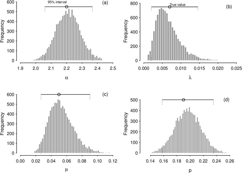
Figure 3: Marginal posterior distributions for the four model parameters and the predictive distributions for the total and observed number of casualties for the simulation study. For each marginal distribution, a 95% prediction interval and the true value is shown. In all cases, the true value is within the posterior distribution.

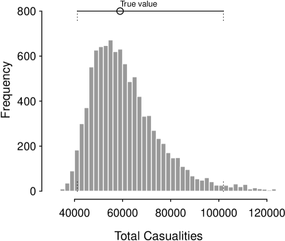
Figure 4: The predictive distribution for the total number of casualties in the simulation study.

After a pilot run to estimate the random walk tuning parameters, we ran the MCMC algorithm (described in Section 3.2), for $1.1$ million iterations. The first $100,000$ iterations were removed as burn-in and the remainder thinned by a factor of $100$ iterations. This yielded a sample of $10,000$ iterates with low auto-correlation to be used as the main monitoring run. See the supplementary material for additional diagnostic plots (Gillespie (2017)).

The posterior densities for the four parameters are given in Figure 3, a–d. The true value is within the 95% credible region for each parameter.

Integrating over parameter uncertainty, we obtain a posterior predictive distribution for the true number of casualties (figure 4). As might be expected, there is considerable uncertainty in the total number of casualties. In particular, there is a relatively long tail which is a result of the underlying power law distribution. However, the true value is still within the 95% credible region.

3.4 Application to the American Indian war

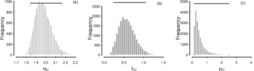
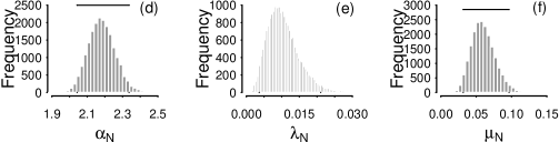
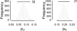
Figure 5: Marginal posterior distributions for the model parameters. For each distribution, a 95% prediction interval. The subscripts $U$ and $N$ denote the US and Native American forces respectively.

Similar to the simulation study, a pilot MCMC run for each force was used to estimate sensible transition kernel tuning parameters. The overall acceptance rate was around $9\%$. The parameters $\alpha$, $\lambda$ and $\mu$ are highly correlated, with a pairwise correlation coefficient of $r\simeq 0.8$. We ran the MCMC algorithm for $2.1$ million iterations; discarding the first $100,000$ iterations and thinning the remainder by a factor of $100$. The total simulation time was around $9$ hours. See the supplementary material for additional diagnostic plots (Gillespie (2017)).

The results for the US and Native American data sets, denoted with sub-scripts $U$ and $N$ respectively, are given in figure 5. For both data sets, the power law scaling parameter is around $\alpha\simeq 2.1$, with $\alpha_{N}<\alpha_{U}$. Intuitively, this makes sense since most casualties on each side would be low level, and the maximum number of casualties in a single event would be approximately the same for both sides.

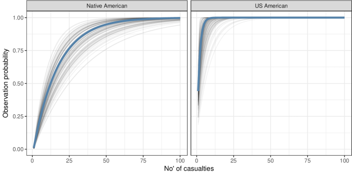
Figure 6: The probability of observing an event. The blue lines give the posterior mean estimate for the observation line. The light grey lines are $100$ samples from the posterior.

The parameters modeling the probability of observing an event considerably differ between the two groups. Figure 6 plots the probability of recording an event. One hundred samples from the posterior have been plotted, in addition to the average probability. The posterior mean probability of observing an event of size $1$ is $E(1-e^{-\lambda}|z)\simeq 0.010$, for the Native Americans, but is significantly larger for the US Americans ($0.46$); where $z$ are the observed battles. The parameter governing the rate at which we perfectly record events, $\mu$, is also larger for the US forces. Related, the posterior mean estimate of $n_{true}$, which is $2,287$ and $20,551$ for the US and Native American forces respectively. For comparison, $n_{obs}$ was $1,232$ and $1,297$.

We can obtain a quasi-estimate of $x_{\min}$, that is, the point where we are unlikely to miss a battle, by calculating

$$x_{0.95}=\arg\min_{x}(E(1-\exp\{-\lambda-\mu(x-1)\}|z)>0.95)\;,$$

where the posterior expectation is calculated using samples from the posterior. This gives point estimates of $x_{0.95}=10$ and $x_{0.95}=57$ for the US and Native American forces, respectively.

As might be expected, rounding or heaping is more prevalent for the Native American forces, with the probability of rounding almost twice as large as for the US American forces (see figure 5 (g, h)).

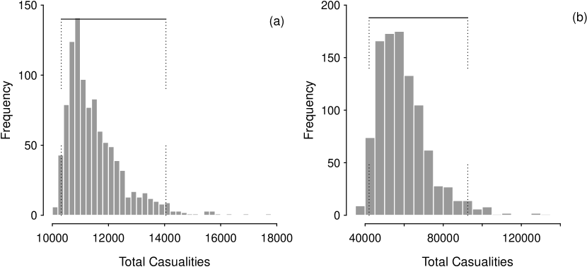
Figure 7: Predictive distributions for the observed and total number of casualties for the US and Native American forces, respectively. For each distribution, a 95% prediction interval is shown.

We can use samples from the posterior distribution to infer the total number of casualties. Figure 7 shows the predicted number of total casualties sustained by each side. Clearly there is a more uncertainty in the Native American casualties (as also demonstrated in figure 5), with the mean number of casualties being around $11,500$ and $60,000$. These numbers are larger than the corresponding power law analysis of Friedman (2015), who estimated $12,000$ and $53,000$ respectively. The reason for the difference is two fold. First, Friedman ignored other sources of error; in particular rounding which is significant in the Native American forces. Second, when estimating uncertainty in the parameters, Friedman used a bootstrap procedure, whereas in this analysis, we condition on what has already been observed. The difference in analysis is noticeable when comparing figure 3 of Friedman (2015) with figure 7. In the bootstrap version, there is considerable distributional mass for casualty estimates less than $40,000$. Some of the bootstrapped samples also suggested that the casualties have been over-estimated, which seems highly unlikely.

3.5 Model fit and sensitivity

As with any Bayesian analysis, it is important to assess the sensitivity of the posterior to the prior specification. Although the prior on the power law coefficient was bounded (this study used a $U(1.5,3)$ prior) the maximum accepted value during the MCMC algorithm was less than $2.5$. Similarly, the prior for the heaping coefficient $p$ was flat. The parameters governing the missing observations did contain more information. However, switching to uniform priors on $\mu$ and $\lambda$ did not substantially effect casualty inferences, but did make tuning the MCMC algorithm more difficult.

A different functional form for the observation probability could also be used. We investigated a quadratic form

$$1-\exp\{-\lambda-\mu(x-1)-\eta(x-1)^{2}\}$$

and a logistic function

$$\frac{1}{1+\exp(-\mu x)}\;.$$

For each of these functions, the overall conclusions were similar with inferences regarding $\alpha$ and $p$ being relatively unaffected.

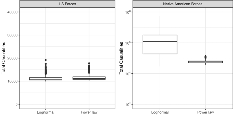
Figure 8: Predictive distributions for the number of casualties for the US and Native American forces, under the log normal and power law models. The power law data is the same as figure 6.Note the change of scale in the Native American casualties.

To capture data rounding, the model only considers multiplies of five. However, examining the Native American casualties, the two largest events were $1,000$ and $2,000$ individuals. It therefore seems likely that for larger events, rounding was occurring to the nearest $100$ or $1,000$. However, there are few large events occurring and so we decided against modelling this, and just note that the overall estimates are unlikely to be affected by this omission.

Perhaps the strongest assumption that we made was assuming that the true underlying distribution was a power law. This assumption was based on the distribution of more recent conflicts. To assess the strength of this assumption, we investigated how the prediction of the total number of casualties altered if we assumed a (discrete) log normal distribution. Using uniform priors for the log normal parameters and the same MCMC scheme as described previously, we obtained the predictions given in figure 8. The predicted number of casualties for the US forces are broadly similar to the results in figure 7. The Native American forces has many more extreme points in the log normal analysis, with the median number of predicted casualties increasing from $66$ thousand to around a million casualties. However, the extreme results are due to the perhaps unreasonable flat priors used for the log normal priors. Interestingly, the estimate of the rounding parameters for each force are relatively unaffected when switching to a log normal distribution.

4 Discussion

In many disparate research areas, underlying processes may generate events on different orders of magnitude. In particular, since the system operates at different levels, modelling the entire mechanism is difficult and so researchers focus on the tail of the distribution. However, by purely focusing on the tail region, it becomes more difficult to incorporate an error model.

This article builds on the work of Friedman (2015) who used the power law structure for prediction. However, by estimating directly $x_{\min}$, it made extending the analysis more complicated when considering more realistic error structures.

The American Indian war play a central role in the history of the United states. However, due to missing data it has been difficult to quantify the number lives lost during this time period. This article provides estimates for the number casualties suffered by both sides. We estimate that the US forces suffered around $12,000$ casualties in this conflict. As Friedman (2015) notes, this is approximately equal to the combined totals of the War of Independence, the War of 1812, the Mexican-American War, and the Spanish- American War. The Native Americans suffered far greater losses, around $60,000$. Since the Native American population was around $400,000$ at the start of the conflict, the number of casualties was catastrophic. To put this number into context, as crude average, suppose the casualties are distributed equally throughout the $115$ year conflict. This results in approximately $0.15\%$ of total population dying in the conflict each year. This is an order of magnitude more than the United States lost in World War 2.

In this paper we modelled the available data and accounted for the different sources of uncertainty. While this resulted in a more complex analysis, it also yields more detailed insights, such as the amount of rounding in each data set. Of course as Friedman (2015) points out, we do not need power laws or sophisticated statistics to establish that the American Indian war were catastrophic for the Native Americans. Indeed, it has been suggested that up to 20 million Native Americans died as result of disease (Pinker, 2011). This analysis attempts to better quantify the number of casualties associated with armed conflicts.

The problem tackled in this paper does not provide a definite answer. Instead, it relies heavily on expert opinion and insight. By building a more structured model and using the Bayesian paradigm, we are able to channel prior beliefs about the probability of observing events and the structure of the underlying model into a predictive framework. The techniques described in this paper could be applied to more recent conflicts, such as Iraq. Where it is difficult to assess number of casualties sustained due to missing data.

The salient, but obvious, point raised in this paper, is that we rarely observe data without error. The error structure could be as simple as Normal perturbations to the true process, or something more complex as described in this paper. Regardless, it is important to consider the impact on our inferences if we ignore the underlying error structure. Indeed, many of the examples considered in the original CSN paper have clearly been observed with error. By switching to a Bayesian analysis, we have been able to properly account for the different sources of error.

Computing details

All simulations were performed on a machine with 4GB of RAM and with an Intel quad-core CPU using R (R Core Team and R Development Core Team, 2013). The CSN power law fits were obtained using the poweRlaw package (Gillespie, 2015). All code associated with this paper can be obtained from

https://github.com/csgillespie/plbayes

References

- Abramowitz and Stegun (1970) {barticle}[author] \bauthor\bsnmAbramowitz, \bfnmMilton\binitsM. and \bauthor\bsnmStegun, \bfnmIrene A\binitsI. A. (\byear1970). \btitleHandbook of Mathematical Function with Formulas, Graphs, and Mathematical Tables. \bjournalNational Bureau of Standards, Applied Mathematics Series \bvolume55. \endbibitem
- Alstott, Bullmore and Plenz (2014) {barticle}[author] \bauthor\bsnmAlstott, \bfnmJeff\binitsJ., \bauthor\bsnmBullmore, \bfnmEd\binitsE. and \bauthor\bsnmPlenz, \bfnmDietmar\binitsD. (\byear2014). \btitlepowerlaw: A Python Package for Analysis of Heavy-Tailed Distributions. \bjournalPLoS ONE \bvolume9 \bpagese85777. \bdoi10.1371/journal.pone.0085777 \endbibitem
- Axelrod (1993) {bbook}[author] \bauthor\bsnmAxelrod, \bfnmAlan\binitsA. (\byear1993). \btitleChronicle of the Indian wars: from colonial times to Wounded Knee. \bpublisherKonecky & Konecky. \endbibitem
- Bell et al. (2012) {barticle}[author] \bauthor\bsnmBell, \bfnmM. J.\binitsM. J., \bauthor\bsnmGillespie, \bfnmC. S.\binitsC. S., \bauthor\bsnmSwan, \bfnmD.\binitsD. and \bauthor\bsnmLord, \bfnmP.\binitsP. (\byear2012). \btitleAn approach to describing and analysing bulk biological annotation quality: A case study using UniProtKB. \bjournalBioinformatics \bvolume28 \bpagesi562–i568. \bdoi10.1093/bioinformatics/bts372 \endbibitem
- Bohorquez et al. (2009) {barticle}[author] \bauthor\bsnmBohorquez, \bfnmJ. C.\binitsJ. C., \bauthor\bsnmGourley, \bfnmS\binitsS., \bauthor\bsnmDixon, \bfnmA R\binitsA. R., \bauthor\bsnmSpagat, \bfnmM\binitsM. and \bauthor\bsnmJohnson, \bfnmN. F.\binitsN. F. (\byear2009). \btitleCommon ecology quantifies human insurgency. \bjournalNature \bvolume462 \bpages911–4. \bdoi10.1038/nature08631 \endbibitem
- Breiman, Stone and Kooperberg (1990) {barticle}[author] \bauthor\bsnmBreiman, \bfnmLeo\binitsL., \bauthor\bsnmStone, \bfnmCharles J\binitsC. J. and \bauthor\bsnmKooperberg, \bfnmCharles\binitsC. (\byear1990). \btitleRobust confidence bounds for extreme upper quantiles. \bjournalJournal of Statistical Computation and Simulation \bvolume37 \bpages127–149. \endbibitem
- Cederman (2003) {barticle}[author] \bauthor\bsnmCederman, \bfnmL. E.\binitsL. E. (\byear2003). \btitleModeling the size of wars: from billiard balls to sandpiles. \bjournalAmerican Political Science Review \bvolume97 \bpages135–150. \endbibitem