Extinction spectra of suspensions of microspheres: Determination of spectral refractive index and particle size distribution with nanometer accuracy

Abstract

A method is presented to infer simultaneously the wavelength-dependent real refractive index (RI) of the material of microspheres and their size distribution from extinction measurements of particle suspensions. To derive the averaged spectral optical extinction cross section of the microspheres from such ensemble measurements, we determined the particle concentration by flow cytometry to an accuracy of typically 2% and adjusted the particle concentration to ensure that perturbations due to multiple scattering are negligible. For analysis of the extinction spectra we employ Mie theory, a series-expansion representation of the refractive index and nonlinear numerical optimization. In contrast to other approaches, our method offers the advantage to simultaneously determine size, size distribution and spectral refractive index of ensembles of microparticles including uncertainty estimation.

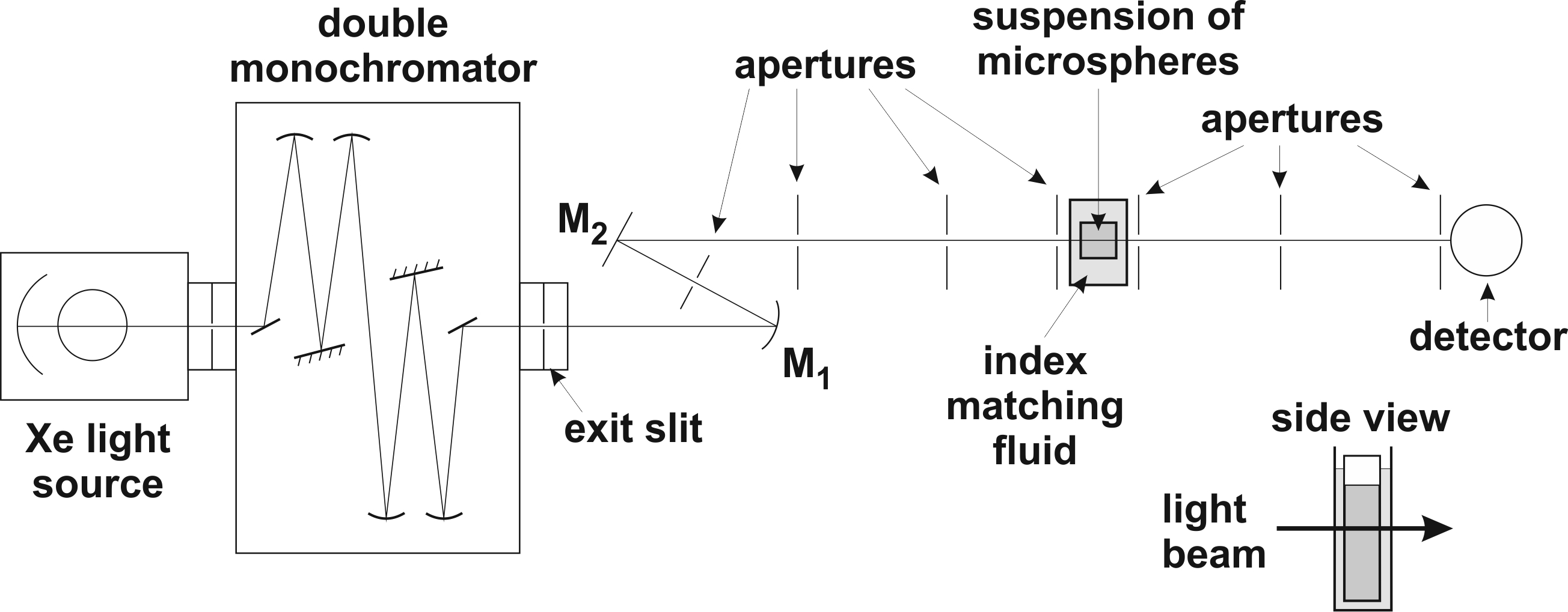
Figure 1: Schematic of experimental setup to measure spectral extinction cross sections of suspensions of spheres.

I Introduction

The refractive index (RI) describes the refraction of a beam of light at a (macroscopic) interface between any two materials. Consequently, a variety of experimental methods exist for measuring the RI of a material that rely on the refraction or reflection of light at a planar interface between the sample and some other known material, such as air, water or an optical glass. This approach is feasible for materials that can exhibit macroscopically large defined interfaces, such as bulk liquids, homogeneous solids or thin films and permits RI measurements with high accuracy. For example, the refractive index of synthetic calcium fluoride has been determined with high accuracy between $138\text{\,}\mathrm{n}\mathrm{m}$ and $2326\text{\,}\mathrm{n}\mathrm{m}$ Daimon and Masumura (2002) and for distilled water Daimon and Masumura (2007) applying the minimum deviation method. However, in many cases one is interested in the optical properties of materials that do not have a homogeneous macroscopic form, such as atmospheric aerosols Jones et al. (1994a, b); Thomas et al. (2005), soot particles in flames Felske and Ku (1992), biological cells or tissues Naumenko et al. (1982); Ma et al. (2003) or man-made nanoparticles Khlebtsov et al. (2008). Often times, these materials cannot be condensed into a homogeneous bulk sample. If the size is comparable to the wavelength of visible light, media containing these particles (e. g., a suspension of cells or a cloud) are turbid, i. e., light is scattered in a complex process instead of propagating in straight rays. Nevertheless, the interaction of light waves with such materials is still determined by the optical and geometrical properties of the constituting particles. It is thus reasonable to ask the question “What is the RI of the small particles contained in the inhomogeneous sample?”. This RI can yield information about the chemical composition of the particles or can be used for further mathematical modeling of light scattering processes. For similar purposes, one is interested in the size of the particles under consideration, e. g., to calculate the force exerted by an optical trap Sun et al. (2008); Stilgoe et al. (2008), For certain cases both properties can be inferred from measurements of the scattering and absorption of light by the particles.

A reference case is that of homogeneous spheres described by a single refractive index, since an analytical solution for the mathematical problem of light scattering exists for this class of particles (Mie theory) Mie (1908); Bohren and Huffman (1983). This makes the analysis of light scattering data feasible and at the same time is a good approximation for many real-world situations. Thus far, several techniques to infer the RI or the size of spherical or small particles from measurements of the scattering or extinction of light have been discussed in the literature Naumenko et al. (1982); Felske and Ku (1992); Jones et al. (1994a, b); Nefedov et al. (1997); Ma et al. (2003); Thomas et al. (2005); Khlebtsov et al. (2008); Zhang et al. (2015); Blümel et al. (2016) These techniques can be divided into those relying on the angular scattering pattern at a single wavelength Naumenko et al. (1982); Jones et al. (1994a, b); Nefedov et al. (1997), and into those techniques relying on spectra of extinction or diffuse transmittance Ma et al. (2003); Thomas et al. (2005); Khlebtsov et al. (2008); Zhang et al. (2015); Blümel et al. (2016). Of course, a combination of these techniques is also possible Felske and Ku (1992).

The inference problem or inverse problem “What is the RI and size distribution for a given extinction spectrum?” is generally challenging. Because the samples used and quantities measured for the various approaches described in the literature are so different, researchers have come up with tailor-made solutions for their particular fields of application. For example, in Ref. 8, the authors used combined collimated and diffuse transmittance measurements to determine the RI of polystyrene spheres of known size. In Ref. 5, the authors analyzed atmospheric aerosols of variable chemical composition. The complex refractive index was restricted to those functions represented by a multi-band damped-harmonic-oscillator model. This allowed to retrieve the RI of the aerosols. However, the approach was unable to represent asymmetric dispersion features. The method described in Ref. 9 was developed for nanoparticles and consequently could be applied only to particles of sub-wavelength size. Measurements in different suspending media were required for RI determination. The authors of Ref. 16 explicitly analyzed the location of ripples in the extinction spectrum of single microspheres using synchrotron radiation. While the RI could be determined quantitatively from the the relative shape of these ripples, an accurate particle sizing was not possible.

In this work we present a method to infer the wavelength-dependence of the real RI and the particle size distribution, characterized by mean value and standard deviation, from a single measurement of spectral extinction cross section for spherical particles in the Mie scattering regime, i. e., the size is comparable to the wavelength. We exemplify the method for suspensions of microscopic synthetic polystyrene (PS) beads that are widely used in colloidal and optical research, e. g., as a calibration material for cell measurements in optical and impedance flow cytometry Frankowski et al. (2015) or attached as “handles” to optically manipulate biological cells Svoboda and Block (1994). From the measurement of an extinction spectrum in the UV-VIS range with a tabletop experimental setup, one can infer the refractive index with an accuracy of 2 to 4 decimal places, depending in the wavelength, as well as the size parameters with accuracies in the range of one nanometer.

II Materials, methods and models

II.1 Experiment

II.1.1 Experimental Setup

To determine spectral extinction cross sections of polystyrene microspheres we measured the collimated transmission of particle suspensions using the setup depicted in Fig. 1. As light source a $1\text{\,}\mathrm{k}\mathrm{W}$ Xenon high pressure discharge lamp is mounted to a double monochromator (model 1680 double spectrometer, SPEX industries, Inc., USA, NJ), equipped with a $1200\text{\,}\mathrm{g}\mathrm{r}\,\mathrm{m}\mathrm{m}^{-1}$ grating for the wavelength range from $185\text{\,}\mathrm{n}\mathrm{m}$ to $900\text{\,}\mathrm{n}\mathrm{m}$. The focal length of the double monochromator is $22\text{\,}\mathrm{c}\mathrm{m}$. When measuring the collimated transmission of particle suspensions, the scanning range was reduced to $260\text{\,}\mathrm{n}\mathrm{m}$–$800\text{\,}\mathrm{n}\mathrm{m}$. Outside this wavelength region, the signal to noise ratio was insufficient, since below $260\text{\,}\mathrm{n}\mathrm{m}$ the output power of the Xe high pressure lamp is too low and above $800\text{\,}\mathrm{n}\mathrm{m}$ the sensitivity of the photomultiplier tube (model R928, Hamamatsu Photonics Deutschland GmbH, Germany) significantly drops. The slit width was set to obtain a spectral resolution of $0.5\text{\,}\mathrm{n}\mathrm{m}$ and the wavelength increment amounted to $1\text{\,}\mathrm{n}\mathrm{m}$. Spectra were recorded with an integration time of $1\text{\,}\mathrm{s}$ and a scanning speed of $0.5\text{\,}\mathrm{n}\mathrm{m}\,\mathrm{s}^{-1}$. Hence, the total measurement time was $18\text{\,}\mathrm{m}\mathrm{i}\mathrm{n}$.

The light emitted from the monochromator was collimated by a spherical mirror of $20\text{\,}\mathrm{c}\mathrm{m}$ focal length ($\mathrm{M_{1}}$) and reflected to the sample cell by a plane mirror ($\mathrm{M_{2}}$). The system of apertures served to minimize the divergence of the light beam and to reduce stray light and ambient light. The adjustable apertures were set to a diameter of $2\text{\,}\mathrm{m}\mathrm{m}$. Taking into account the distance of $90\text{\,}\mathrm{c}\mathrm{m}$ between the first aperture and the aperture directly mounted in front of the cuvette with the index matching fluid, the maximum cone of light that can enter the cuvette is characterized by a half-angle of $0.13\text{\,}\mathrm{\SIUnitSymbolDegree}$. The suspension of microspheres was pipetted in a quartz glass cuvette (type 110-QS, Hellma GmbH & Co. KG, Germany) used for photometric absorption measurements. The path length of the cuvette is $d=$10\text{\,}\mathrm{m}\mathrm{m}$$ with an uncertainty of $u(d)=$10\text{\,}\mathrm{\SIUnitSymbolMicro m}$$. To avoid the influence of slightly different angles when inserting the cuvette in the beam path, which would result in changes in back reflection and transmission, a container filled with index matching oil (Immersol 518N, Carl Zeiss Microscopy GmbH, Germany) was permanently mounted. The size of the container (inner dimensions $$20\text{\,}\mathrm{m}\mathrm{m}$\times$30\text{\,}\mathrm{m}\mathrm{m}$$) was chosen in such a way that the quartz glass cuvettes, featuring outer dimensions of $$12.5\text{\,}\mathrm{m}\mathrm{m}$\times$12.5\text{\,}\mathrm{m}\mathrm{m}$$, could be easily changed. The long distance of $120\text{\,}\mathrm{c}\mathrm{m}$ between the cuvette and the detector, together with a system of adjustable apertures set to $2\text{\,}\mathrm{m}\mathrm{m}$ diameter, served to effectively suppress light scattered at small angles. The half-observation angle amounted to $0.1\text{\,}\mathrm{\SIUnitSymbolDegree}$. As stated above, the transmitted light was recorded using a R928 photomultiplier tube.

II.1.2 Properties of polystyrene microspheres

Diameter and size distribution

To validate the experimental procedure and the associated mathematical model we measured the collimated transmission of two different types of PS microspheres. The mean diameter of the first type (dynospheres™ 50.010.SS-021 P, LOT Q262, Dyno Particles A.S., Norway) – the results are denominated as dataset 1 in the following – was specified as $2.0\text{\,}\mathrm{\SIUnitSymbolMicro}\mathrm{m}$. The stated coefficient of variation of 1.2% corresponds to a standard deviation of $0.024\text{\,}\mathrm{\SIUnitSymbolMicro}\mathrm{m}$. The mass of PS amounted to $0.1\text{\,}\mathrm{g}$ in $10\text{\,}\mathrm{m}\mathrm{L}$. Taking into account the density of PS of $1.05\text{\,}\mathrm{g}\,\mathrm{m}\mathrm{L}^{-1}$ and the particle volume of $4.19\text{\,}\mathrm{f}\mathrm{L}$ the concentration was $c=$2.3\text{\times}{10}^{9}\text{\,}\mathrm{m}\mathrm{L}^{-1}$$. As second sample (dataset 2) we chose microspheres (Flow Check™ microparticles, Cat. No. 23526-10, Polysciences Europe GmbH, Germany) with a slightly different diameter of $2.076\text{\,}\mathrm{\SIUnitSymbolMicro}\mathrm{m}$ and larger standard deviation of $0.053\text{\,}\mathrm{\SIUnitSymbolMicro}\mathrm{m}$ (CV = 2.6%). Since these particles are generally used for calibration purposes in flow cytometry without diluting the sample, the concentration of about $10^{7}\,$\mathrm{m}\mathrm{L}^{-1}$$ is significantly lower compared to the other sample used.

Sedimentation

The influence of sedimentation of the particles during the measurement time of $18\text{\,}\mathrm{m}\mathrm{i}\mathrm{n}$ was estimated by calculating their velocity using Stokes’ law. In equilibrium, the frictional force and the excess force due to the difference in density of water and PS are equal. Using the density of PS $\rho_{\text{PS}}=$1.05\text{\,}\mathrm{g}\,\mathrm{m}\mathrm{L}^{-1}$$ and the dynamic viscosity of water $\mu_{\rm H_{2}O}=$9.321\text{\times}{10}^{-4}\text{\,}\mathrm{k}\mathrm{g}\,\mathrm{m}^{-1}\,\mathrm{s}^{-1}$$ at $23\text{\,}\mathrm{\SIUnitSymbolCelsius}$ the sinking velocity of PS particles with $2\text{\,}\mathrm{\SIUnitSymbolMicro}\mathrm{m}$ diameter amounts to $0.12\text{\,}\mathrm{\SIUnitSymbolMicro}\mathrm{m}\,\mathrm{s}^{-1}$. It follows that the sedimentation path in $18\text{\,}\mathrm{m}\mathrm{i}\mathrm{n}$ is about $0.13\text{\,}\mathrm{m}\mathrm{m}$. This value is negligible, since the light beam is positioned in the middle of the cuvette, the filling height of which is typically $2\text{\,}\mathrm{c}\mathrm{m}$, and the depletion zone as well as the enrichment zone are in a distance of about $1\text{\,}\mathrm{c}\mathrm{m}$.

RI of bulk polystyrene and water

For the analysis of the experimental spectral extinction cross sections initial values are needed for the wavelength dependence of the refractive index of the PS microspheres. To this end, we employ literature values for the RI of bulk PS and water, shown in Fig. 2. The data for the PS RI from Ref. 19 can be fitted very well using a one-term Sellmeier equation containing a single absorption pole. We used this extrapolation curve to generate synthetic data for the spectral range [260, 800] $\mathrm{n}\mathrm{m}$. For the wavelength-dependent RI of pure water we used a four-term Sellmeier equation Daimon and Masumura (2007) that is accurate to a few ${10}^{-6}$ in the wavelength range $182\text{\,}\mathrm{n}\mathrm{m}$–$1129\text{\,}\mathrm{n}\mathrm{m}$. The absorbance of water in the wavelength range under consideration is very low and can thus be neglected, hence $n_{\rm H_{2}O}\in\mathbb{R}$. The same basically holds for PS, however, there is the onset of a (weak) UV absorption line at $4.5\text{\,}\mathrm{e}\mathrm{V}$ or $275\text{\,}\mathrm{n}\mathrm{m}$ Inagaki et al. (1977). Nevertheless, we treat its RI as real-valued.

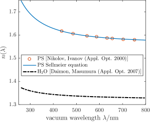
Figure 2: Refractive index of water Daimon and Masumura (2007) and polystyrene Nikolov and Ivanov (2000). To create synthetic data, the data for PS was extrapolated from the measured range $436\text{\,}\mathrm{n}\mathrm{m}$–$1052\text{\,}\mathrm{n}\mathrm{m}$ to the near UV by the Sellmeier equation shown as a blue solid line.

II.1.3 Sample preparation and transmittance measurements

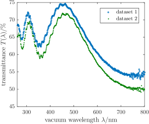
Figure 3: Transmission spectrum of polystyrene microspheres with a diameter of approximately $2\text{\,}\mathrm{\SIUnitSymbolMicro}\mathrm{m}$.

The mathematical model for the analysis of extinction spectra requires that only single scatter events occur when the light passes the cuvette. Multiple scattering is not included. To ensure that this condition is met, the concentration of particles is chosen correspondingly and measured by a flow cytometer, designed to determine reference values for concentrations of blood cells and particles in suspensions Ost et al. (1998); Reitz et al. (2010). The mean free path length between two scattering events was estimated by taking two times the geometrical cross section as optical extinction cross section. For a transmittance of, e. g., 70% the mean free path length of $30\text{\,}\mathrm{m}\mathrm{m}$ exceeds the cuvette path length by a factor of 3. For the samples the dilution was adjusted to yield concentrations $c$ of $(4.95\pm 0.09)\times{10^{6}}\,$\mathrm{m}\mathrm{L}^{-1}$$ and $(5.23\pm 0.10)\times 10^{6}\,$\mathrm{m}\mathrm{L}^{-1}$$ for datasets 1 and 2, respectively. In Fig. 3, we depict the result of measurements of the spectral transmission for the two datasets. These spectra represent the transmittance of the particle suspensions, since blank values were corrected. To this end, we first measured the transmittance $I_{0}(\lambda)$ of the cuvette with pure water. Subsequently, the cuvette was cleaned and filled with the particle suspension. The transmittance $I(\lambda)$ of the suspension was measured and the spectral transmittance derived as ratio between both measurements:

$$T(\lambda)=\frac{I(\lambda)}{I_{0}(\lambda)}.$$ (1)

It should be noted that all measurements were normalized to the spectral output power of the monochromator using the quantum absorber Melhuish (1972) integrated in the instrument.

The spectral transmittance can also be expressed as

$$T=\exp\left(-\frac{C_{\text{ext}}^{\text{ensemble}}}{\Omega}\right),$$ (2)

where $\Omega$ is the area illuminated by the beam. $C_{\text{ext}}^{\text{ensemble}}$ is the extinction cross section of the particle ensemble. The particles in the sample are specified by the manufacturer as monodisperse, since generally the variation in size is negligible for the intended purpose, e. g., calibration of flow cytometers. However, spectral extinction is sensitive to the size variation and consequently we have to consider the particles as polydisperse. Because we are dealing with incoherent single scattering events, the total extinction cross section of the ensemble of $\nu$ particles is the sum of the single particles’ extinction cross sections

$$C_{\text{ext}}^{\text{ensemble}}=\sum_{j=1}^{\nu}C_{\text{ext}}^{j}.$$ (3)

With the optical path length of $d=$10\text{\,}\mathrm{m}\mathrm{m}$$, the particle concentration of $c\approx$5\text{\times}{10}^{6}\text{\,}\mathrm{m}\mathrm{L}^{-1}$$ and the area $\Omega=$3.1\text{\,}\mathrm{m}\mathrm{m}^{2}$$ given by a $2\text{\,}\mathrm{m}\mathrm{m}$ aperture, the number of particles $\nu=\Omega\,d\,c$ is on the order of $10^{5}$. This allows for the measurement of an ensemble average, denoted by

$$\overline{C}_{\text{ext}}=\frac{1}{\nu}\,C_{\text{ext}}^{\text{ensemble}}=-\ln\left(\frac{I}{I_{0}}\right)\,\frac{1}{d\,c}.$$ (4)

The path length $d$ is known to a relative accuracy of $10^{-3}$ and the particle concentration $c$ was measured using flow cytometry to a relative standard deviation of 2%. The latter uncertainty contribution thus introduces an uncertainty into the scaling factor for the measured ensemble average in Eq. (4). In the following, we drop the subscript ${}_{\text{ext}}$, i. e., $\overline{C}_{\text{ext}}=\overline{C}$ and denote experimental data by an asterisk: $\overline{C}^{*}$.

II.1.4 Noise model for cross section measurements

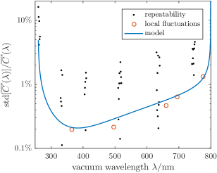
Figure 4: Estimates of the coefficient of variation $\hat{\sigma}[\overline{C}^{*}\!(\lambda)]$ due to measurement noise: Maximal estimate from repeated measurements (black dots), minimal estimate from local fluctuations of $\overline{C}^{*}\!(\lambda)$ (red circles) and model curve [Eq. (6), blue line].

There are different sources of measurement uncertainty: (1) concentration uncertainties as discussed above, (2) detector noise, and (3) possible other systematic influences yet to be determined. The latter point is discussed in subsection II.2.3.

We assume the detector noise to be white (i. e., uncorrelated between different wavelengths), to have a wavelength-dependent amplitude $\mathrm{std}[\overline{C}^{*}\!(\lambda)]$, and a coefficient of variation

$$\hat{\sigma}[\overline{C}^{*}\!(\lambda)]=\frac{\mathrm{std}[\overline{C}^{*}\!(\lambda)]}{\overline{C}^{*}\!(\lambda)}.$$ (5)

We estimated $\hat{\sigma}[\overline{C}^{*}\!(\lambda)]$ from the data in two different ways:

1. From the variation of repeated measurements for the same sample in overlapping spectral regions, which yields an upper bound of the statistical measurement error, because it also contains systematic contributions resulting from drift of measurement conditions and other sources. The estimated $\hat{\sigma}[\overline{C}^{*}\!(\lambda)]$ has a characteristic “bathtub shape” (Fig. 4), which we approximate by a function

   $$\hat{\sigma}[\overline{C}^{*}\!(\lambda)]=\frac{p_{1}}{\sqrt{p_{2}^{2}-(\lambda-p_{3})^{2}}}+p_{4}\,\lambda+p_{5}.$$ (6)

   with five fit parameters. Such a shape indicates increased noise contributions due to low output power of the light source in the UV and a decreasing sensitivity of the detector for long wavelengths.

2. From the local fluctuations of $\overline{C}_{\text{ext}}$ in regions of vanishing slope, which yields an estimate of the measurement error. Due to the pronounced ripple structure of the data, no estimate is possible at the blue end of the spectrum and the bathtub shape is not resolved. We use the same model function [Eq. (6)] as for the estimate based on the variation of repeated measurements above and simply rescale it by a factor $<1$ to optimally fit the minimal error estimate. The resulting curve is shown in Fig. 4 and is used for weighting and uncertainty analysis in the following.

II.2 Mathematical model

II.2.1 Mie scattering

The scattering particles are assumed to be spherical and multiple scattering effects are negligible due to the low particle concentration and low sample thickness. Mathematically, the experiment can thus be described using the time-harmonic Maxwell equations for the scattering of a plane electromagnetic wave by a single homogeneous sphere. This problem has an analytic solution, which is known as Mie theory or Mie scattering Mie (1908); Bohren and Huffman (1983). Mie scattering yields the full electric field for the scattering problem as a series expansion in vector spherical harmonics, from which, among other quantities, the total extinction cross section $C_{\text{ext}}$ can be computed. The problem is fully characterized by two parameters:

1. The size parameter

   $$X:=\frac{2\pi\,n_{\rm m}}{\lambda}\,R,$$

   where $R$ is the radius of the sphere, $\lambda$ is the wavelength in vacuo and $n_{\rm m}\in\mathbb{R}$ is the RI of the (non-absorbing) medium (water), respectively.

2. The relative refractive index

   $$\mathfrak{m}:=\frac{\mathfrak{n}}{n_{\rm m}}\in\mathbb{C},$$

   where $\mathfrak{n}=n+\mathrm{i}\kappa\in\mathbb{C}$ is the RI of the sphere. The imaginary part $\kappa$ describes the absorption of light in the sphere’s material.

Consequently, besides the known quantities vacuum wavelength $\lambda$ and RI of the medium $n_{\rm m}(\lambda)$, the two quantities sphere radius $R$ and sphere’s RI $\mathfrak{n}(\lambda)$ are the two free parameters of the system.

Using a numerical implementation of the Mie scattering formulae Wis , accurate values for the extinction cross section of a single particle are easily obtained for any given parameters $\mathfrak{n}(\lambda)$ and $R$ in the relevant range. We denote these numerically obtained values by the function

$$\mathcal{C}(\lambda;\mathfrak{n},R).$$

This notation shall indicate that we are considering a wavelength-dependent function with two parameters, one of which, the RI $\mathfrak{n}(\lambda)$, is a function of the wavelength itself.

II.2.2 Polydisperse ensembles

Since the number of particles measured simultaneously in the experiment is large, the ensemble average in Eq. (4) is modeled by simply integrating over the corresponding size distribution

$$\overline{\mathcal{C}}(\lambda;\mathfrak{n}|r)=\int_{0}^{\infty}\mathcal{C}(\lambda;\mathfrak{n},R)\,r(R)\,\mathrm{d}R,$$ (7)

where $r(R)$ is the probability density function (pdf) of the radius $R$. We model it by a normal distribution

$$r(R)\propto\exp\left\{-\frac{1}{2}\frac{[R/R_{c}-\mu_{R}]^{2}}{\sigma_{R}^{2}}\right\}.$$ (8)

Here $R_{c}$ is a typical length scale (e. g., a rough guess for the mean particle radius), rescaling the parameters to dimensionless quantities of the order of 1. $\mu_{R}$ is the mean and $\sigma_{R}$ the standard deviation of the distribution of radii, relative to the characteristic scale $R_{c}$. We combine these two parameters of the distribution into the vector

$$\bm{\theta}:=(\mu_{R},\sigma_{R})^{T}.$$ (9)

A normal distribution was chosen as a model function since it is known to describe the size distribution of polystyrene microspheres very well Lettieri et al. (1991). Alternatively, we also tested a log-normal distribution. For the narrow size distributions of the samples used here, the difference in shape between a normal distribution an a log-normal distribution of identical mean value and standard deviation is only minor. Consequently, the results were virtually the same in both cases.

To implement the integrals in the ensemble average numerically, we used trapezoidal sums over uniform grids, with appropriate spacing and range.

II.2.3 Correction for systematic influences

Including concentration errors in the forward model for the measured curve would result in the ensemble averaged $\overline{\mathcal{C}}(\lambda;\mathfrak{n}|r)$ being multiplied with a prefactor $1-\epsilon_{c}$, where $\epsilon_{c}$ corresponds to the relative concentration error with $\mathbb{E}(\epsilon_{c})=0$, $\mathrm{std}(\epsilon_{c})\approx 2\%$. However, it turns out that the forward model is much more flexible and the quality of the solution of the inverse problem can be greatly enhanced when a simple parametric wavelength dependence of this prefactor is introduced, i. e., instead of $1-\epsilon_{c}$, we have $1-\epsilon_{c}+\epsilon_{o}(\lambda;\bm{\eta})$, where $\epsilon_{o}(\lambda;\bm{\eta})$ corrects for influences other than the concentration. Mathematically, the influences of concentration and other factors can not be distinguished, hence we merge them into a single wavelength-dependent function $\epsilon(\lambda;\bm{\eta})=-\epsilon_{c}+\epsilon_{o}(\lambda;\bm{\eta})$. This compensation curve is characterized by the parameters $\bm{\eta}=(\eta_{1},\dotsc,\eta_{m_{\eta}})^{T}$ and defined as a linear interpolation between a few grid points

$$\epsilon(\lambda;\bm{\eta}):=\begin{cases}\eta_{j}&\lambda=l_{j}\\ \text{linearly interpolated }&\text{between the }l_{j}\\ \eta_{1}&\lambda<l_{1}\\ \eta_{M_{\eta}}&\lambda>l_{M_{\eta}}\end{cases},$$ (10)

with $l_{1}<\dots<l_{M_{\eta}}$, $\bm{\eta}=(\eta_{1},\dotsc,\eta_{M_{\eta}})^{T}$. A small number of points ($M_{\eta}=4$ in our case) is sufficient to significantly improve the quality of the fit compared to the one obtained with a constant function. Hence, our model for the measured $\overline{C}^{*}\!(\lambda_{j})$ is

$$\mathcal{M}(\lambda;\mathfrak{n},\bm{\theta},\bm{\eta}):=[1+\epsilon(\lambda;\bm{\eta})]\,\overline{\mathcal{C}}(\lambda;\mathfrak{n}|r).$$ (11)

From a physical point of view, this wavelength-dependent factor serves to correct for one or several influences, which are difficult to quantify here, in particular aspects such as non-sphericity as well as the finite-size detector aperture and the beam divergence. From a mathematical point of view, the introduction of $\epsilon(\lambda;\bm{\eta})$ is justified by the much higher quality of the fit. As will be discussed in section III, we obtain more convincing results for the fitted RI and size distribution using this correction.

For a choice of the grid points $l_{1},\dotsc,l_{M_{\eta}}$ we tested uniform grids as well as a random placement using $M_{\eta}=0..10$ points. However, the best results (measured by the quality of the fit) were obtained when the local minima and maxima of the slow oscillations of $\overline{C}^{*}\!(\lambda)$ were selected, which are at $300\text{\,}\mathrm{n}\mathrm{m}$, $350\text{\,}\mathrm{n}\mathrm{m}$, $450\text{\,}\mathrm{n}\mathrm{m}$ and $770\text{\,}\mathrm{n}\mathrm{m}$ for $2\text{\,}\mathrm{\SIUnitSymbolMicro}\mathrm{m}$ PS spheres in water (Fig. 6).

II.3 Inverse problem

We now have a mathematical model for the measurement and are able to compute the average extinction cross section for a given ensemble of spheres, i. e., for a given size distribution and RI $n(\lambda)$. We assume $\mathfrak{n}(\lambda)=\Re\left[\mathfrak{n}(\lambda)\right]=n(\lambda)$ here and in the following due to polystyrene’s negligible absorbance.

The question we now address is: Can one infer the RI $n(\lambda)$ from measurements $\left[\overline{C}^{*}\!(\lambda_{j})\right]_{j=1}^{N}$? First of all, it is clear that one should not try to infer more than $N$ parameters from $N$ given measurement data. This leaves the possibility to obtain $n(\lambda_{j})$ for all $\lambda_{j},j=1..N$, given knowledge about the size distribution and particle concentration, which is a relatively simple problem: At each wavelength $\lambda_{j}$, find $n_{j}=n(\lambda_{j})$, such that

$$\overline{\mathcal{C}}(\lambda_{j};n_{j}|r)\stackrel{{\scriptstyle!}}{{=}}\overline{C}^{*}\!(\lambda_{j}).$$ (12)

The problem is hence stated as finding roots of a nonlinear equation for all wavelengths separately. Hence, this approach is pointwise. However, as it turns out, the pointwise approach fails: Slight, sub-percent errors in the size distribution or in the particle concentration strongly affect the result of the RI reconstruction and Eq. (12) may not even have solutions any more for some wavelengths. Since the prior knowledge about the parameters of the size distribution is not accurate enough, they need to be inferred from the data as well. At first glance, this leaves one with more parameters to be reconstructed than data points. But the problem can be restated in a non-pointwise sense as a least-squares optimization problem.

II.3.1 Representation of $n(\lambda)$

We restate the problem by implying a constraint on the admissible functions $n$, namely that they can be expressed as a finite sum of smooth basis functions $g_{j}$, i. e.,

$$n(\lambda)=\sum_{j=1}^{M}a_{j}g_{j}(\lambda)\quad\forall\,\lambda\in\mathbb{R}$$ (13)

with unknown coefficients $a_{j}$. Hence, we are working in the subspace spanned by the $M$ basis functions with $M<N$.

Simple oscillator models for light-matter interactions reveal that particles with a resonance at wavelength $\Lambda>0$ and of width $\gamma>0$ exhibit an anomalous dispersion feature described by the expression

$$n(\lambda)-1\propto\frac{\lambda-\Lambda}{(\lambda-\Lambda)^{2}+\gamma^{2}},$$ (14)

which is thus a generic shape of a feature of the real part of the RI. Hence, we represent the refractive index $n(\lambda)$ in a sparse form by working in the $M$-dimensional space

$$n\in\mathrm{span}\{1,f_{1},\dotsc,f_{M-1}\},$$ (15)

where

$$f_{j}(\lambda):=\frac{\lambda-y_{j}}{(\lambda-y_{j})^{2}+\gamma^{2}}.$$ (16)

The centers of the peaks $y_{j}$ are uniformly spaced, i. e., $y_{j}-y_{j-1}=\Delta_{y}$. We chose a grid spacing of $\Delta_{y}=$30\text{\,}\mathrm{n}\mathrm{m}$$ and a constant width of $\gamma=$100\text{\,}\mathrm{n}\mathrm{m}$$ for all functions. The first (last) grid point was set to be one grid spacing $\Delta_{y}$ smaller (larger) than the lowest (highest) wavelength.

These functions $f_{i}$ are linearly independent, but they are not useful for a practical implementation, since they are far from being orthogonal, i. e., the scalar products between them are not close to zero, which would lead to problems in the numerics. To avoid this problem, we orthonormalize the set of functions $\{1,f_{1},\dotsc,f_{M-1}\}$, or rather the set the values of these functions at $(\lambda_{1},\dotsc,\lambda_{N})$, using the (modified) Gram-Schmidt process, yielding an orthonormal set $\{g_{1},\dotsc,g_{M}\}$, i. e.,

$$\langle g_{i},g_{j}\rangle=\delta_{ij}\text{\quad{}and\quad}g_{1}(\lambda_{j})=\frac{1}{\sqrt{N}}\;\forall\,j=1,..,N,$$ (17)

where $\langle.\,,.\rangle$ denotes the standard inner product in $\mathbb{R}^{N}$.

This representation of $n(\lambda_{j})$ as a series expansion in adequately-chosen basis vectors results in a reduction of the dimensionality by a factor of 30: Instead of one coefficient every $1\text{\,}\mathrm{n}\mathrm{m}$ corresponding to the spectral resolution, only one coefficient every $30\text{\,}\mathrm{n}\mathrm{m}$ is needed. At the same time, it is possible to represent the RI of bulk PS (Fig. 2) to machine precision. But also curves less generic than this Sellmeier equation (see footnote ), e. g., the feature-rich spectral RI of the protein complex hemoglobin Friebel and Meinke (2006); Gienger et al. (2016) can be represented with errors well below the respective measurement uncertainties using an appropriate grid spacing $\Delta_{y}$.

II.3.2 Nonlinear least-squares optimization

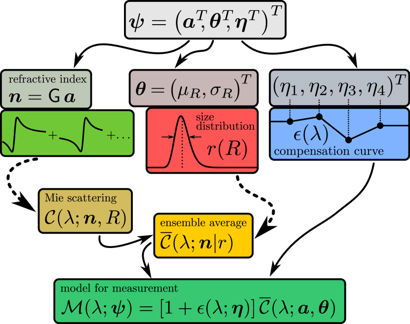
Figure 5: Schematic representation of the mathematical model of the experiment. Linear transformations are shown as solid lines, nonlinear dependencies as dashed lines.

The series expansion of the real RI in Eq. (13) can also be written as a matrix-vector product

$$\bm{n}=\mathsf{G}\,\bm{a}$$ (18)

with $\mathsf{G}:=\{g_{j}(\lambda_{i})\}_{i,j}\in\mathbb{R}^{N\times M}$, $\bm{n}=(n(\lambda_{1}),\dotsc,n(\lambda_{N}))^{T}$. The coefficient vector $\bm{a}$ describing the RI, the vector $\bm{\theta}$ describing the size distribution of the spheres and vector $\bm{\eta}$ describing the compensation curve are the unknown quantities which we need to recover from the spectral extinction data. Thus we combine them into a single parameter vector

$$\bm{\psi}:=\begin{pmatrix}\bm{a}\\ \bm{\theta}\\ \bm{\eta}\end{pmatrix}\in\mathbb{R}^{L},$$ (19)

where $L=27$ with the parameters chosen for measurement data discussed here ($N=540$ points). The mathematical forward model to compute the extinction cross sections $\mathcal{M}(\lambda;\bm{\psi})$ from the parameter vector $\bm{\psi}$ is depicted in Fig. 5.

We then set up a quadratic cost function consisting of the summed squared residuals

$$F_{i} :=\mathcal{M}(\lambda_{i};\bm{\psi})-\overline{C}^{*}(\lambda_{i})$$ (20)

$$\chi^{2}(\bm{\psi}) :=\sum_{i,j=1}^{N}w_{ij}F_{i}F_{j}=\bm{F}^{T}\,\mathsf{W}\,\bm{F},$$ (21)

where $\mathsf{W}=\mathsf{V}(\bm{\overline{C}^{*}})^{-1}$ is a symmetric weight matrix with

$$\mathsf{V}(\bm{\overline{C}^{*}})=\mathrm{diag}(\sigma_{1}^{2},\dotsc,\sigma_{N}^{2}).$$ (22)

The standard deviations $\sigma_{i}=\mathrm{std}[\overline{C}^{*}\!(\lambda_{i})]$ are estimated according to Eq. (6) for each dataset. The necessary condition for optimal parameters that minimize $\chi^{2}$ is then

$$0\stackrel{{\scriptstyle!}}{{=}}\nabla_{\bm{\psi}}\chi^{2}(\bm{\psi})=\mathsf{J}^{T}\nabla_{\bm{F}}\chi^{2}(\bm{\psi})=2\,\mathsf{J}^{T}\mathsf{W}\bm{F},$$ (23)

where we have introduced the Jacobian matrix

$$\mathsf{J}=\left\{\frac{\partial F_{i}}{\partial\psi_{j}}\right\}_{ij}\in\mathbb{R}^{N\times L}.$$ (24)

Further details for the implementation of the forward model are given in Appendix A. Numerically, the necessary condition can be solved by iterative local optimization methods. We tested both the Levenberg-Marquardt algorithm and the trust-region-reflective algorithm as they are implemented in Matlab (MATLAB R2016a, The MathWorks, Inc.). Both algorithms basically yield the same result when converged. Since the trust-region-reflective algorithm proved more stable with respect to the choice of initial values, all the results presented here were obtained with this algorithm. When converged, the numerical routine yield an optimal parameter set $\hat{\bm{\psi}}$ corresponding to a local minimum and $\chi^{2}$ normalized to the degrees of freedom

$$\chi^{2}_{\rm dof}:=\frac{\chi^{2}(\hat{\bm{\psi}})}{N-L+1}$$ (25)

provides a measure for the quality of the fit.

Influence of initial parameter values

The local nonlinear optimization employed for the same dataset can result in different estimates of the parameter vector $\bm{\psi}$ when different initial values are used. Firstly, it is possible that the found local minimum is far away from true parameter values (for synthetic data) or plausible parameter values (for experimental data). This is usually indicated by a large value of $\chi^{2}_{\rm dof}$ (i. e., $\chi^{2}_{\rm dof}\gg 1$). Secondly, one can also find different local minima rather close to each other and – in the case of synthetic data – similarly close to the correct value, indicating multiple minima of the least-squares problem. For these minima further iteration does not improve the fit. We estimated the resulting uncertainty stemming from this effect as follows: Different initial parameter values were created by adding normally distributed random numbers to the same mean initial parameter vector. We tuned the amplitude of these random numbers such that the range of initial conditions is sufficiently wide and that, on the other hand, the optimization converged for the majority of samples. However, very high values of $\chi^{2}_{\rm dof}$ do occur in some cases. In order to include all of these samples appropriately, we introduced weights proportional to $\exp(-\chi^{2}_{\rm dof})$ in the averages and covariances over the ensemble of optimization runs. This penalty term attenuates samples with poor agreement between model and data (e. g., $\chi^{2}_{\rm dof}=10$). The result for the parameter vector is then obtained as the weighted average $\langle\bm{\psi}\rangle_{\text{init}}$ over the ensemble of random initial parameter values.

The uncertainty analysis for the estimated parameters is presented in Appendix B.

III Results

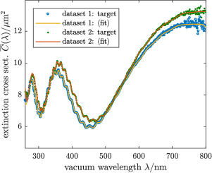
Figure 6: Experimental extinction cross sections (“target”) and model fits with optimized parameters as described in subsections II.2 and II.3. See Data Files 1 and 2 for underlying values of the respective datasets.

III.1 Inverse problem results

To evaluate the method, we created synthetic datasets for polystyrene particles suspended in pure water. These synthetic data were created as follows: The optical properties assumed are shown in Fig. 2. The compensation curve was fixed to $\epsilon(\lambda;\bm{\eta})\equiv 0$ in the forward model and Gaussian white noise was added according to the coefficient of variation estimated in Eq. (6) and shown in Fig. 4. We analyzed synthetic data with $\mathrm{mean}(R)=$1\text{\,}\mathrm{\SIUnitSymbolMicro m}$$, $\mathrm{std}(R)=$5\text{\,}\mathrm{n}\mathrm{m}$$ for different realizations of measurement noise and observed that the deviations of the found size distribution parameters were within the margins expected from the corresponding estimated uncertainties. We computed the difference between the RI values $n(\lambda_{j})$ obtained by optimization and those according to the target curve. The percentages of values within one (two) standard deviation(s) estimated from the uncertainty analysis were found to be close to the 68% (95%) one expects from a normal distribution, indicating a reasonable estimate of the uncertainties. Generally, these percentages were even higher, indicating that the uncertainties are slightly overestimated. The compensation curve also returned the target ($\bm{\eta}=0$) within the uncertainties.

The experimental cross sections, i. e., datasets 1 and 2 (Fig. 6), were analyzed in the same way. The resulting RI is depicted in Fig. 7 (a) and the corresponding uncertainty (Fig. 7 (b)) is shown to be less than 1% almost everywhere and to be less than 0.1% between $300\text{\,}\mathrm{n}\mathrm{m}$ and $650\text{\,}\mathrm{n}\mathrm{m}$. The compensation curve is shown in Fig. 7 (c). The wavelength-dependence of $\epsilon(\lambda;\bm{\eta})$ is significant with the estimated uncertainties. Tab. 1 lists the mean values and standard deviations of the particle size distributions. All these results correspond to the MC-averaged optimized parameters.

Table 1: Optimization results for size distribution parameters, cf. Fig. 7. The numbers in parentheses are the standard uncertainties referred to the last digits of the respective results.

	$\mathrm{mean}(R)/$\mathrm{n}\mathrm{m}$$	$\mathrm{std}(R)/$\mathrm{n}\mathrm{m}$$
dataset 1
result	$1015.1(8)$	$4.7(2)$
specification	$1000$	$12$
dataset 2
result	$1038.5(9)$	$4.4(2)$
specification	$1038$	$27$

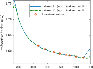
(a)

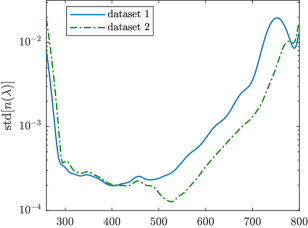
(b)

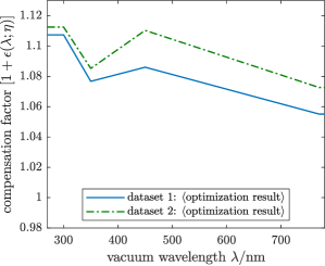
(c)

Figure 7: Optimization results for the model parameters for $2\text{\,}\mathrm{\SIUnitSymbolMicro m}$ PS spheres for two experimental datasets: (a) Refractive index. Literature values are from Ref. 19. The oscillations of $n(\lambda)$ at the red and UV end of the spectrum are within the estimated uncertainties (Fig. 7 (b)). See Data Files 1 and 2 for underlying values of the respective datasets. (b) Estimated uncertainties (one standard deviation) of the RI (Fig. 7 (a)). (c) Compensation curve. The piecewise linear function $\epsilon(\lambda;\bm{\eta})$ is spanned by 4 grid points at $300\text{\,}\mathrm{n}\mathrm{m}$, $350\text{\,}\mathrm{n}\mathrm{m}$, $450\text{\,}\mathrm{n}\mathrm{m}$ and $770\text{\,}\mathrm{n}\mathrm{m}$.

For wavelengths larger than $436\text{\,}\mathrm{n}\mathrm{m}$, we compared the RI uncertainties with the deviations between the found RI curves and the Sellmeier curve for the literature RI of bulk PS (see footnote ). For the first dataset 52% (65%) of the values were within one (two) estimated standard deviations of the literature values. For the second dataset 37% (57%) were within one (two) standard deviations. Although these percentages are somewhat too low, it indicates that the estimated uncertainties are not too far off. Furthermore, these numbers do not take into account any uncertainties of the RI literature values or possible deviations of the RI of PS microspheres in our samples from that of bulk PS.

As an additional consistency test, we computed the difference between the RI curves obtained independently from the two experimental datasets. This difference was within the combined estimated uncertainties, thus indicating that the uncertainty estimates are reliable.

III.2 Effect of the compensation curve

In Fig. 8 (a) we plot the local extinction-cross-section residuals $F(\lambda_{j};\bm{\psi})=\mathcal{M}(\lambda_{j};\bm{\psi})-\overline{C}^{*}(\lambda_{j})$ as a function of wavelength and refractive index. We performed an additional optimization with a forward model not including the compensation curve, i. e., $\bm{\eta}\equiv 0$ in the optimization. The result is shown in Fig. 8 (b). Comparing Figs. 8 (a) and (b), ones sees how the incorporation of $\epsilon(\lambda;\bm{\eta})$ into the model enables it to close the gaps that are otherwise present near the local extrema of $\overline{C}^{*}\!(\lambda)$ (compare Fig. 6). The ripples in $\overline{C}^{*}\!(\lambda)$ are not matched by the model fit (data not shown) and for dataset 1 we obtained $\langle\chi^{2}_{\rm dof}\rangle=7.3$ (indicating a poor fit) instead of $\langle\chi^{2}_{\rm dof}\rangle=0.78$ (indicating a very good fit) with the forward model including $\epsilon(\lambda;\bm{\eta})$. For dataset 2 these values were $\langle\chi^{2}_{\rm dof}\rangle=10.6$ and $\langle\chi^{2}_{\rm dof}\rangle=1.57$, respectively. Furthermore, the curves for $n(\lambda)$ obtained for datasets 1 and 2 do not match each other within the estimated uncertainties in the former case and neither of them matches the literature data. In conclusion, the optimization with the forward model including $\epsilon(\lambda;\bm{\eta})$ (i. e., in our example with $L=27$ free parameters instead of $L=23$) yield much more consistent and plausible results than with the one not including $\epsilon(\lambda;\bm{\eta})$ and thus was chosen even though the physical origin of the effect cannot be identified unambiguously.

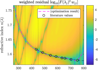
(a)

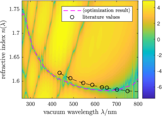
(b)

Figure 8: Dataset 1: Residuals $F(\lambda_{j};\bm{\psi})=\mathcal{M}(\lambda_{j};\bm{\psi})-\overline{C}^{*}(\lambda_{j})$ of the extinction cross section as a function of wavelength and assumed refractive index. The parameters $\bm{\theta}$ and $\bm{\eta}$ are fixed to the optimization result. (a) With forward model incorporating the compensation curve $\epsilon(\lambda;\bm{\eta})$ (Fig. 5). The black dotted lines denote the wavelength grid spanning $\epsilon(\lambda;\bm{\eta})$ (Fig. 7 (c)). Note the false solutions intersecting at the local extrema of $\overline{C}^{*}\!(\lambda)$ (Fig. 6) and the blurred valley at the red end due to measurement noise. (b) With forward model not incorporating the compensation curve $\epsilon(\lambda;\bm{\eta})$.

III.3 Reliability of solutions for wider ensembles

The procedure for solving the inverse problem and related uncertainty analysis works well for the cases discussed here with $\mathrm{mean}(R)\approx$1\text{\,}\mathrm{\SIUnitSymbolMicro m}$$ and $\mathrm{std}(R)/\mathrm{mean}(R)\approx 0.5\%$, i. e., for a narrow size distribution. Using synthetic data, however, we found that the parameter retrieval becomes increasingly difficult for wider size distributions. This is because the characteristic ripples in $\overline{C}(\lambda)$ get smoothed out for wider size distributions. This ripple structure is very sensitive to particle size and RI Blümel et al. (2016). Hence, when this characteristic fine structure is suppressed by ensemble averaging essential information is lost. The effects of RI, mean radius and particle concentration in the model can then compensate each other, which can lead to a good fit of $\overline{C}(\lambda)$ with systematically incorrect parameters. To quantify this, we analyzed synthetic data with $\mathrm{mean}(R)=$1\text{\,}\mathrm{\SIUnitSymbolMicro m}$$ and distribution widths of $0.1\%\leq\mathrm{std}(R)/\mathrm{mean}(R)\leq 5.0\%$. Without added measurement noise, the correct parameters can be found in all cases, i. e., this is not a problem of (numerical) sensitivity in the forward model. In the presence of measurement noise, however, systematic parameter errors occur for values of $\mathrm{std}(R)/\mathrm{mean}(R)\geq 1\%$, because in these cases the sensitivity is obscured by measurement noise. These deviations typically increase with distribution width. A similar effect can also be expected for low-contrast particles, because this attenuates the ripple structure as well. This problem could in principle be resolved by achieving a sufficiently low measurement noise.

IV Summary and discussion

We presented measurements of the spectral extinction cross sections of polystyrene microspheres suspended in water. Theses measurements $\overline{C}^{*}\!(\lambda)$ represent averages over the size distribution of the polydisperse ensemble. Using a numerical implementation of Mie scattering, in combination with an appropriate description of the size distribution and the spectral refractive index $n(\lambda)$ in a low-dimensional set of orthonormal basis functions, we developed a forward model $\mathcal{M}(\lambda;\bm{\psi})$ to mathematically describe the measurements for a given parameter set $\bm{\psi}$. Applying standard nonlinear least-squares optimization, the $L$ model parameters contained in the vector $\bm{\psi}$ were fitted to $N$ measurement data points. In our example, we had $N=540$ and $L=27$. This yields the spectral refractive index of the microspheres, the mean value of their size and the standard deviation of their size distribution. The uncertainties of these results were estimated using linearized propagation of covariance matrices and Monte Carlo sampling.

The wavelength dependence of the RI of PS microspheres derived by modeling experimental extinction cross sections including uncertainties yields results consistent with literature values. This good accordance proves that the microspheres are produced with a homogeneity in density and optical properties that is comparable to bulk material. On the other hand, both samples feature about the same size distribution with a coefficient of variation of about 0.5%, which is significantly lower than the specification of the vendors of 1.2% and 2.6%, respectively. It follows that the particles are closer to monodispersity than declared, presumably since the specified distribution widths are estimates of the corresponding upper limit during production.

The method for measurement and data analysis presented here allows to determine the mean diameter of an ensemble of $2\text{\,}\mathrm{\SIUnitSymbolMicro m}$ PS spheres with an uncertainty of $2\text{\,}\mathrm{n}\mathrm{m}$ or a relative uncertainty of $10^{-3}$. This uncertainty was estimated from the measurement noise and the limited precision of the inverse problem’s solution and verified with synthetic data. Model errors might have an additional effect not analyzed here, e. g., deviations from a spherical shape or surface roughness. However, since even the most intricate details of the extinction spectra, i. e., their ripple structure, can be fitted with the model, it seems unlikely that surface roughness is relevant. The scattering properties from ensembles of rough spheres have been examined Schiffer (1989, 1990) and it was found that the deviations between spheres and rough spheres are largest for side scattering and backscattering amplitudes, whereas forward and near-forward scattering is least sensitive to irregularities. Due to the optical theorem Bohren and Huffman (1983), this means that the extinction cross section $C_{\text{ext}}$ is very insensitive to irregularities of the particles’ surfaces. Hence the Mie scattering formulae may be used even for somewhat irregular particles.

We have demonstrated the potential of spectral extinction measurements in combination with an adapted mathematical model to determine microparticle properties. To further improve the model, in particular for new applications, the investigations will be extended to particles in the size range of several hundred nanometers up to about $10\text{\,}\mathrm{\SIUnitSymbolMicro}\mathrm{m}$ and to other (non-absorbing and absorbing) materials. In addition, comparison with complementary methods used to determine size and size distribution, i. e., dynamic light scatter, secondary electron microscopy, nanoparticle tracking and sedimentation analyses will be carried out.

Potential applications of our spectral extinction measurement and analysis method include quality assurance to monitor size, size distribution and composition (i. e., spectral RI) when producing suspensions of nano- and micro-particles or emulsions. The method is also sensitive towards the homogeneity of the particles (e. g., quartz spheres) and allows to identify irregularities by comparing the spectral RI of the particles to the RI of the bulk material. Complementarily, the roles of medium and particle RI can be interchanged in the optimization. In this way, the spectral RI of the solvent, e. g., a protein solution, can be deduced using (monodisperse) micro-spheres with known optical and morphological parameters as a probe.

Appendix A Expressions for the numerical implementation of optimization

The ensemble-averages with trapezoidal sums replacing integrals read

$$\overline{\mathcal{C}}(\lambda_{i};\bm{\psi}) =\sum_{t=1}^{I}\mathcal{C}(\lambda_{i};\mathfrak{n}_{i}(\bm{a}),R_{t})\,\tilde{r}_{t}(\bm{\theta}).$$ (26)

For the Jacobian matrix one finds

$$J_{ij}=\frac{\partial F_{i}}{\partial\psi_{j}} =\begin{cases}[1+\epsilon(\lambda;\bm{\eta})]\frac{\partial\overline{\mathcal{C}}(\lambda_{i};\bm{a},\bm{\theta})}{\partial\psi_{j}}&j=1..L-M_{\eta}\\ \frac{\partial\epsilon(\lambda;\bm{\eta})}{\partial\psi_{j}}\overline{\mathcal{C}}(\lambda_{i};\bm{a},\bm{\theta})&\text{else}\end{cases},$$ (27)

with

$$\frac{\partial\overline{\mathcal{C}}(\lambda_{i};\bm{a},\bm{\theta})}{\partial a_{j}} =\sum_{t=1}^{I}\left[\frac{\partial}{\partial\mathfrak{n}_{i}}\mathcal{C}(\lambda_{i};\mathfrak{n}_{i},R_{t})\right]\,\tilde{r}_{t}\,\frac{\partial\mathfrak{n}_{i}}{\partial a_{j}}$$

$$=\sum_{t=1}^{I}\left[\frac{\partial}{\partial\mathfrak{n}_{i}}\mathcal{C}(\lambda_{i};\mathfrak{n}_{i},R_{t})\right]\,\tilde{r}_{t}\,G_{ij}$$ (28)

$$\frac{\partial\overline{\mathcal{C}}(\lambda_{i};\bm{a},\bm{\theta})}{\partial\theta_{j}} =\sum_{t=1}^{I}\mathcal{C}(\lambda_{i};\mathfrak{n}_{i}(\bm{a}),R_{t})\,\frac{\partial}{\partial\theta_{j}}\tilde{r}_{t}(\bm{\theta})$$ (29)

A partial derivative like $\frac{\partial}{\partial\mathfrak{n}_{i}}\mathcal{C}(\lambda_{i};\mathfrak{n}_{i},R)$ can be computed numerically by finite differences at the same computational complexity as $\mathcal{C}(\lambda_{i};\mathfrak{n}_{i},R)$. The derivatives $\frac{\partial\epsilon(\lambda;\bm{\eta})}{\partial\eta_{j}}$ are trivial because of the linear dependence of $\epsilon$ on $\bm{\eta}$. The Jacobian matrix $\mathsf{J}$ is thus implemented efficiently using the above equations and was used explicitly in the numerical optimization.

Appendix B Uncertainty analysis

The sources of measurement uncertainties of $\overline{C}^{*}\!(\lambda)$ and estimates thereof were given in subsection II.1.4. We now analyze the uncertainties of the resulting parameters obtained by nonlinear optimization. There are two types of uncertainty contributions:

1. A contribution due to the measurement uncertainties of the experimental data $\overline{C}^{*}\!(\lambda)$. Here we focus on detector noise since concentration uncertainties and the compensation curve are included explicitly in the forward model. We will denote the terms related to the measurement uncertainty by a superscript “meas”.

2. A contribution from the local least-squares optimization, denoted by a superscript “init”. It describes the uncertainty arising from the ambiguity of the solution when starting the parameter optimization from different initial values.

We estimated both contributions using the direct sampling Monte Carlo (MC) method as described in the following.

B.1 Propagation of measurement uncertainties

The contribution of measurement uncertainties is estimated by linearized covariance-matrix propagation according to

$$\mathsf{V}^{\text{meas}}(\bm{\psi})=\left[\mathsf{J}^{T}\,\mathsf{V}^{\text{meas}}(\bm{\overline{C}^{*}})^{-1}\,\mathsf{J}\right]^{-1}.$$ (30)

To verify the validity of this linearization of the forward model, we performed MC simulations for synthetic data: A number $N_{\rm MC}$ of synthetic datasets was created by adding independent random realizations of the measurement noise [Eq. (6)] to the same synthetic curve ($\mathrm{mean}(R)=$1\text{\,}\mathrm{\SIUnitSymbolMicro m}$$, $\mathrm{std}(R)=$5\text{\,}\mathrm{n}\mathrm{m}$$, $\epsilon\equiv 0$). For each of these random datasets, the inverse problem was solved numerically using the same initial parameter values. The covariance matrix of the optimized parameter vector $\bm{\psi}$ was estimated for each of these numerical solutions according to Eq. (30) and an average was taken over the $N_{\rm MC}$ samples. In addition, we estimated $\mathsf{V}^{\text{meas}}(\bm{\psi})$ using the statistical sample covariance over the set of MC samples. In this setup, the two independent estimates are consistent, thus legitimating the linearized propagation of measurement uncertainties, also for experimental data with similar parameters.

B.2 Uncertainties from initial values

As described in subsection II.3.2 the result for the parameter vector is estimated as the weighted average from $N_{\text{init}}$ optimization runs with random initial values

$$\langle\bm{\psi}\rangle_{\text{init}}:=\frac{1}{Z_{1}}\sum_{i=1}^{N_{\text{init}}}\beta_{i}\,\bm{\psi}^{(i)}$$ (31)

with weights $\beta_{i}:=\exp\left[-\chi^{2}_{\rm dof}\left({\bm{\psi}}^{(i)}\right)\right]$ and $Z_{s}:=\sum_{i}{\beta_{i}}^{s},s\in\mathbb{N}$. $\bm{\psi}^{(i)}$ is the optimization result of the $i$th run. From these statistical ensembles, we further estimated the covariance

$$\mathsf{V}^{\text{init}}(\langle\bm{\psi}\rangle_{\text{init}}) :=$$

$$\frac{Z_{2}}{{Z_{1}}^{2}-Z_{2}}\,\frac{1}{Z_{1}}\sum_{i=1}^{N_{\text{init}}}\beta_{i}\,\left(\bm{\psi}^{(i)}-\langle\bm{\psi}\rangle_{\text{init}}\right)\left(\bm{\psi}^{(i)}-\langle\bm{\psi}\rangle_{\text{init}}\right)^{T},$$ (32)

which can be applied to both, experimental and synthetic data (keeping the realization of measurement noise identical in all samples). The total parameter variance corresponding to the combined uncertainty of measurement and data analysis is then

$$\mathsf{V}(\langle\bm{\psi}\rangle_{\text{init}})=\left\langle\mathsf{V}^{\text{meas}}(\bm{\psi})\right\rangle_{\text{init}}+\mathsf{V}^{\text{init}}(\langle\bm{\psi}\rangle_{\text{init}}).$$ (33)

For a sufficiently large number of samples, the “initial” term will ultimately scale like $\mathsf{V}^{\text{init}}\propto 1/\sqrt{N_{\text{init}}}$. Using $N_{\text{init}}=50$, the computing time was a few minutes on a year 2014 desktop PC and $\mathsf{V}^{\text{init}}$ indeed became almost negligible.

From the parameter covariance $\mathsf{V}(\langle\bm{\psi}\rangle_{\text{init}})$ we can easily extract the uncertainty of the spectral refractive index $\bm{n}=\mathsf{G}\,\bm{a}$ as

$$\mathsf{V}(\langle\bm{n}\rangle_{\text{init}})=\mathsf{G}\,\mathsf{V}(\langle\bm{a}\rangle_{\text{init}})\,\mathsf{G}^{T},$$ (34)

where $\mathsf{V}(\langle\bm{a}\rangle_{\text{init}})$ corresponds to the first $M\times M$ entries of $\mathsf{V}(\langle\bm{\psi}\rangle_{\text{init}})$, and analogously for the other resulting parameters.

Initial parameter values

For analyzing $2\text{\,}\mathrm{\SIUnitSymbolMicro m}$ PS particles, the initial values were chosen as follows ($\mathrm{mean}\pm 1\mathrm{std}$ of Gaussian white noise):

1. The RI was initialized as a piecewise-linear function spanned over the points $n[(260,460,800)\,$\mathrm{n}\mathrm{m}$]=(1.75,1.605,1.585)$, which is a crude approximation of the Sellmeier curve (Fig. 2). For the MC sampling, the coefficient vector varied $\bm{a}$ with a standard deviation of 0.6 for $a_{1}$ and 0.04 for $a_{j},j=2,...,M$, respectively.

2. The mean radius $\mathrm{mean}(R)$ was initialized to $$1000\text{\,}\mathrm{n}\mathrm{m}$\pm$20\text{\,}\mathrm{n}\mathrm{m}$$ and the distribution width $\mathrm{std}(R)$ to $$10\text{\,}\mathrm{n}\mathrm{m}$\pm$4\text{\,}\mathrm{n}\mathrm{m}$$.

3. The compensation curve was initialized with $\eta_{j}=0.00\pm 0.05$.

References

- Daimon and Masumura (2002) M. Daimon and A. Masumura, Appl. Opt. 41, 5275 (2002), URL http://ao.osa.org/abstract.cfm?URI=ao-41-25-5275.
- Daimon and Masumura (2007) M. Daimon and A. Masumura, Appl. Opt. 46, 3811 (2007).
- Jones et al. (1994a) M. R. Jones, B. P. Curry, M. Q. Brewster, and K. H. Leong, Appl. Opt. 33, 4025 (1994a), URL http://ao.osa.org/abstract.cfm?URI=ao-33-18-4025.
- Jones et al. (1994b) M. R. Jones, K. H. Leong, M. Q. Brewster, and B. P. Curry, Appl. Opt. 33, 4035 (1994b), URL http://ao.osa.org/abstract.cfm?URI=ao-33-18-4035.
- Thomas et al. (2005) G. E. Thomas, S. F. Bass, R. G. Grainger, and A. Lambert, Appl. Opt. 44, 1332 (2005), URL http://ao.osa.org/abstract.cfm?URI=ao-44-7-1332.
- Felske and Ku (1992) J. D. Felske and J. C. Ku, Combustion and Flame 91, 1 (1992), ISSN 0010-2180, URL http://www.sciencedirect.com/science/article/pii/0010218092901237.
- Naumenko et al. (1982) E. K. Naumenko, T. V. Oleinik, and A. Y. Khairullina, Optics and Spectroscopy 53, 288 (1982).
- Ma et al. (2003) X. Ma, J. Q. Lu, R. S. Brock, K. M. Jacobs, P. Yang, and X.-H. Hu, Physics in Medicine and Biology 48, 4165 (2003), URL http://stacks.iop.org/0031-9155/48/i=24/a=013.
- Khlebtsov et al. (2008) B. N. Khlebtsov, V. A. Khanadeev, and N. G. Khlebtsov, Langmuir 24, 8964 (2008), pMID: 18590302, eprint http://dx.doi.org/10.1021/la8010053, URL http://dx.doi.org/10.1021/la8010053.
- Sun et al. (2008) B. Sun, Y. Roichman, and D. G. Grier, Opt. Express 16, 15765 (2008), URL http://www.opticsexpress.org/abstract.cfm?URI=oe-16-20-15765.
- Stilgoe et al. (2008) A. B. Stilgoe, T. A. Nieminen, G. Knöner, N. R. Heckenberg, and H. Rubinsztein-Dunlop, Opt. Express 16, 15039 (2008), URL http://www.opticsexpress.org/abstract.cfm?URI=oe-16-19-15039.
- Mie (1908) G. Mie, Annalen der Physik 330, 377 (1908).
- Bohren and Huffman (1983) C. F. Bohren and D. R. Huffman, Absorption and Scattering of Light by Small Particles (Wiley, 1983).
- Nefedov et al. (1997) A. P. Nefedov, O. F. Petrov, and O. S. Vaulina, Appl. Opt. 36, 1357 (1997), URL http://ao.osa.org/abstract.cfm?URI=ao-36-6-1357.
- Zhang et al. (2015) Y. Zhang, Y. Zhang, X. Han, P. Tuersun, and K. F. Ren, Procedia Engineering 102, 315 (2015), ISSN 1877-7058, new Paradigm of Particle Science and Technology Proceedings of The 7th World Congress on Particle Technology, URL http://www.sciencedirect.com/science/article/pii/S1877705815001496.
- Blümel et al. (2016) R. Blümel, M. Bağcioğlu, R. Lukacs, and A. Kohler, J. Opt. Soc. Am. A 33, 1687 (2016), URL http://josaa.osa.org/abstract.cfm?URI=josaa-33-9-1687.
- Frankowski et al. (2015) M. Frankowski, P. Simon, N. Bock, A. El-Hasni, U. Schnakenberg, and J. Neukammer, Engineering in Life Sciences 15, 286 (2015), ISSN 1618-2863, URL http://dx.doi.org/10.1002/elsc.201400078.
- Svoboda and Block (1994) K. Svoboda and S. M. Block, Annual Review of Biophysics and Biomolecular Structure 23, 247 (1994), pMID: 7919782, eprint https://doi.org/10.1146/annurev.bb.23.060194.001335, URL https://doi.org/10.1146/annurev.bb.23.060194.001335.
- Nikolov and Ivanov (2000) I. D. Nikolov and C. D. Ivanov, Appl. Opt. 39, 2067 (2000), URL http://ao.osa.org/abstract.cfm?URI=ao-39-13-2067.
- Inagaki et al. (1977) T. Inagaki, E. T. Arakawa, R. N. Hamm, and M. W. Williams, Phys. Rev. B 15, 3243 (1977), URL https://link.aps.org/doi/10.1103/PhysRevB.15.3243.
- Ost et al. (1998) V. Ost, J. Neukammer, and H. Rinneberg, Cytometry 32, 191 (1998), ISSN 1097-0320, URL http://dx.doi.org/10.1002/(SICI)1097-0320(19980701)32:3<191::AID-CYTO5>3.0.CO;2-N.
- Reitz et al. (2010) S. Reitz, A. Kummrow, M. Kammel, and J. Neukammer, Measurement Science and Technology 21, 074006 (2010), URL http://stacks.iop.org/0957-0233/21/i=7/a=074006.
- Melhuish (1972) W. H. Melhuish, J. Res. Nat. Bur. Stand. USA 76, 547 (1972).
- (24) For numerical Mie computations we used the Fortran 77 code by W. J. Wiscombe (wiscombe@climate.gsfc.nasa.gov), NASA Goddard Space Flight Center and wrapped it in Matlab.
- Lettieri et al. (1991) T. R. Lettieri, A. W. Hartman, G. G. Hembree, and E. Marx, Journal of research of the National Institute of Standards and Technology 96, 669 (1991).
- Friebel and Meinke (2006) M. Friebel and M. Meinke, Appl. Opt. 45, 2838 (2006).
- Gienger et al. (2016) J. Gienger, H. Groß, J. Neukammer, and M. Bär, Appl. Opt. 55, 8951 (2016), URL http://ao.osa.org/abstract.cfm?URI=ao-55-31-8951.
- Schiffer (1989) R. Schiffer, J. Opt. Soc. Am. A 6, 385 (1989), URL http://josaa.osa.org/abstract.cfm?URI=josaa-6-3-385.
- Schiffer (1990) R. Schiffer, Appl. Opt. 29, 1536 (1990), URL http://ao.osa.org/abstract.cfm?URI=ao-29-10-1536.