Computing by nowhere increasing complexity

Abstract

A cellular automaton is presented whose governing rule is that the Kolmogorov complexity of a cell’s neighborhood may not increase when the cell’s present value is substituted for its future value. Using an approximation of this two-dimensional Kolmogorov complexity the underlying automaton is shown to be capable of simulating logic circuits. It is also shown to capture trianry logic described by a quandle, a non-associative algebraic structure. A similar automaton whose rule permits at times the increase of a cell’s neighborhood complexity is shown to produce animated entities which can be used as information carriers akin to gliders in Conway’s game of life.

I Introduction

In natural and artificial systems pattern formation and order are the imprints of a computational process. We ask whether this process can be reversed – can the enforcement of order or a pattern bring about computation ? What sort of computation can be realized, for example, by not allowing the local patterns in cellular automata to get any more complex than they already are ? Can any computation be realized in such a manner ? This work is an attempt to answer some of these questions.

A cellular automaton is a discrete dynamical system that was originally conceived in the late 1940’s by John von Neumann and Stanislaw Ulam. They incorporated Cellular automaton model into von Neumann’s idea of a “universal constructor” [2]. Cellular automaton exhibits a new way of thinking of how little complexity can achieve interesting behavior, which can be emulated in diverse physical and biological phenomena [3]. They have played a significant role in computation. As has been seen that using Conway’s game of life, for example, they can realize a Turing machine. The idea that the universe in itself is a cellular automaton inspired Zuse’s Calculating Space [4], a precursor of digital physics.

A typical cellular automaton consists of a grid of cells each storing a value and a set of rules according to which their values change. Although the underlying rules may be simple, the behavior of the automaton as a whole may quickly become complex, a trait that allows such automatons to emulate diverse physical and biological phenomena. There are many known cellular automatons whose chaotic behavior has been intensively studied. Perhaps the most famous are the game of life (Life), and rule 110. It has been shown that both of them can realize any computation an ordinary computer can perform [5].

Von Neumann’s universal constructor used thousands of cells and 29 states to self-reproduce. Its complexity was later on reduced in [6]. Langton constructed a self-replicating automaton known as Langton’s loops [7]. His model is less complex than that of the previous models due to von Neumann and Codd. Langton’s model was further simplified in [8, 9]. The constructions of the smallest computationally universal cellular automata have been considered in [10]. Reversible cellular automaton has been studied in [11]. The links between dynamical and computational properties of cellular automaton have been investigated by Di Lena and Margara [12].

Here we show that computation in cellular automata can be realized by exerting local order, where “order” is mathematically defined in terms of Kolmogorov complexity. In particular, we formulate a cellular automaton that employs the following rule. A cell’s value is changed from $y$ to $x$ if the Kolmogorov complexity of its present Moore neighborhood is smaller with $x$ than with $y$. Using an approximation of this two-dimensional Kolmogorov complexity we show that the underlying automaton can compute Boolean functions. In particular, it can realize a universal set of Boolean gates, AND and NOT, as well as wire elements for transferring information from a given cell to any other cell. This automaton is also shown to capture trinary logic described by a quandle, a non-associative algebraic structure whose axioms have been interpreted as laws of conservation of information [13, 14].

The expressiveness of a cellular automaton employing the “nowhere increasing” complexity rule is rather limited. The initial grid which encodes the logic circuit gradually obliterates during the automaton evolution. This implies that similar constructions may not be used for recursive computations. Nevertheless, a similar automaton with an alternating rule where the cell’s neighborhood complexity may at times increase is shown to produce animated entities which can be used as information carriers akin to gliders in the game of life [15].

This work is organized as follows. The next section is a brief introduction to the notion of Kolmogorov complexity. The underlying cellular automaton is described in Section III. It is shown to realize logic gates in Section IV, and other computations and gliders in Section V. Concluding remarks are offered in the last section.

II Kolmogorov complexity

The Kolmogorov complexity, $K(s)$, of an object or a string $s$, is a measure of the computational resources that are needed to generate $s$ [16, 17]. Informally, $K(s)$ is the length of the shortest program that produces $s$ as an output and then halts. The string $\left(01\right)^{n}$, for example, can be described as “n repetitions of $01$”. This string is $2n$ digits long while its description contains around $\log_{2}\left(n\right)$ binary digits, i.e., the length of the binary representation of $n$. On the other hand, seemingly random occurrences of zeros and ones will generally not admit a description shorter than its own length.

The Kolmogorov complexity can be used to define the measure

$$2^{-K(s)}.$$ (1)

If $K(s)$ is the length of a program to a universal prefix Turning machine that produces $s$ and then halts, then by Kraft’s inequality (1) may be interpreted as an unnormalized measure of probability over all such programs [17].

Kolmogorov complexity is an incomputable function – there is no program which takes a string $s$ as an input and produces the number $K(s)$ [17]. Normally, $K(s)$ is approximated using known compression techniques, see e.g., [18]. But (1) can also be used to estimate $K(s)$, assuming one can simulate a large number of Turing machines that produce $s$. Some of these machines will halt and some won’t. Counting the number of them that produced $s$ and then halted gives a number $m(s)$. The Kolmogorov complexity is then approximated, up to a constant, as $-\log_{2}m(s)$ [19, 20].

In this work we are interested in the Kolmogorov complexity of a two-dimensional object, a $3\times 3$ binary matrix. As explained in the next section such a matrix describes the Moore neighborhood of a cell. The complexity of all these 512 binary matrices have been recently approximated in [20]. Simulating a large number of two-dimensional Turing machines the probability (1) was approximated for any given matrix configuration. An estimate of $K$ was then obtained as described above. These approximations can be found at \https://github.com/algorithmicnaturelab/ OACC/blob/master/data/K-3x3.csv

III The cellular automaton

A cellular automaton is defined by a finite number of “colored” cells together with a set of rules that specify how to manipulate their colors. The cells of a standard automaton contain binary values, either “0” (black) or “1” (white). The purpose of the rules is to determine the state (color) of a cell at time $t+1$ based on the values of its neighbors, the set of cells in its vicinity at time $t$. The automaton evolves by using the rules to determine the next value for each cell in the grid at time $t$. The new cell values thus obtained make the grid at time $t+1$.

Let us denote $c_{ij}(t)\in\{0,1\}$, the value at time $t$ of the cell whose coordinates are $\left(i,j\right)$. At each time step a cell updates its value according to the following rule.

Rule: A cell’s value is changed from $c$ to $1-c$ if the Kolmogorov complexity of its present Moore neighborhood is smaller with $1-c$ than with $c$.

This rule is mathematically expressed by:

$$c_{ij}(t+1)=\left\{\begin{array}[]{ll}c_{ij}(t),&K_{ij}(t)\leq K^{\prime}_{ij}(t)\\ 1-c_{ij}(t),&\text{otherwise}.\end{array}\right.$$ (2)

Here, $K_{ij}(t)$ is the Kolmogorov complexity at time $t$ of the Moore neighborhood of $c_{ij}(t)$, a $3\times 3$ pattern composed of the cell at location $(i,j)$ together with 8 other cells that surround it. The Kolmogorov complexity at time $t$ of the same pattern in which the cell at $(i,j)$ is flipped is represented by $K^{\prime}_{ij}(t)$. For example, $K$ and $K^{\prime}$ may be evaluated for the following pair:

A pseudocode for a cellular automaton employing the above rule is provided in Algorithm 1.

Algorithm 1 Nowhere increasing Kolmogorov complexity CA

  Syntax: $c_{ij}(t+1)=\text{\bf CA}\downarrow(c_{ij}(t))$

  Input: $c_{ij}(t)$, $i=1,\ldots,N$, $j=1,\ldots,M$ (grid at time $t$)

  Output: $c_{ij}(t+1)$, $i=1,\ldots,N$, $j=1,\ldots,M$ (grid at time $t+1$)

  for $i=2:N-1$ do

     for $j=2:M-1$ do

        Let $A$ be the Moore neighborhood of $c_{ij}(t)$.

        Obtain $K_{ij}(t)$ using $A$ from the lookup table [20].

        Flip the value of the middle cell in $A$ and similarly obtain $K^{\prime}_{ij}(t)$.

        if $K_{ij}(t)\leq K^{\prime}_{ij}(t)$ then

           $c_{ij}(t+1)=c_{ij}(t)$

        else

           $c_{ij}(t+1)=1-c_{ij}(t)$

        end if

     end for

  end for

IV Computational capabilities

In what follows the underlying automaton is shown to realize the universal set of gates, NOT and AND, together with wire elements for connecting them. By a gate or a wire we mean a grid whose cells store initial values some of which represent inputs and some other represent outputs. Iterating the above automaton rule where $K$ and $K^{\prime}$ are approximated as in [20], changes the cells values. This procedure is reiterated until all cell values no longer change or oscillate indefinitely. The output cells then store the outcome of the computation.

A wire element transfers information between cells in the grid. Its basic form is shown in Figure 1. In this picture the input $x\in\{0,1\}$ to the wire is specified by a single black cell in the block of white cells just above the wire upper end. The wire’s other end is connected to another block of white cells. The initial grids of the automaton for two different inputs $x$ are shown in the leftmost column in this picture. In the upper left frame the black cell in the center of the white block represents the input “0”. Similarly, the input “1” in the lower left frame is represented by a black cell just below the center of this white block. Injecting “0” to the wire completely destructs it, as seen by the upper sequence of shots taken at different times during the evolution. Injecting “1”, the shots in the lower row show a propagating sequence of alternating black and white cells comes out of the upper white block all the way down. These two behaviors are interpreted as a wire carrying either “0” or “1”, i.e., the content of the wire can be read off at the vicinity of $y$.

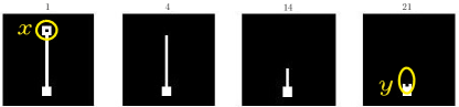
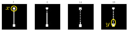
Figure 1: Wire element. The grid size is $30\times 30$.

A NOT gate takes inputs $x$ and returns $y=1-x$. Its realization is shown in Figure 2. The upper row in this picture shows the initial grid for this gate with different inputs, $x=1$ and $x=0$. The respective outputs $y=0$ and $y=1$ in the lower row are obtained after several iterations of the automaton rule.

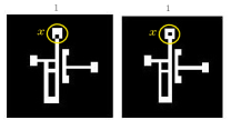
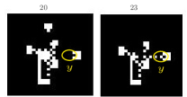
Figure 2: NOT gate. The upper row shows the initial grid for the two inputs, $x=1$ (left) and $x=0$ (right). The respective final grid for each input is shown in the lower row. The grid size is $30\times 30$.

An AND gate takes inputs $x$ and $y$ and returns $z=xy$, i.e., only when $x=y=1$ does the gate returns $z=1$. Its realization is shown in Figure 3. The upper row in this picture shows the initial grid for this gate with different inputs $(x,y)$, i.e., $(0,0)$, $(0,1)$, $(1,0)$, and $(1,1)$. The respective outputs $z=0$, $z=0$, $z=0$, and $z=1$ in the lower row are obtained after several iterations of the automaton rule.

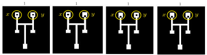
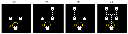
Figure 3: AND gate. The upper row shows the initial grid for the four input combinations, from left to right $(0,0)$, $(0,1)$, $(1,0)$, and $(1,1)$. The respective final grid for each input is shown in the lower row. The grid size is $30\times 30$.

An OR gate may be constructed out of an AND and three NOTs, i.e., $z=1-(1-x)(1-y)$, so that $z=1$ if at least one of the inputs, $x=1$ or $y=1$. The realization of this gate is shown in Figure 4. The upper row in this picture shows the initial grid for this gate with different inputs $(x,y)$, i.e., $(0,0)$, $(1,0)$, $(0,1)$, and $(1,1)$. The respective outputs $z=0$, $z=1$, $z=1$, and $z=1$ in the lower row are obtained after several iterations of the automaton rule. The realization in Figure 5 is that of an XOR gate, for which the output is $z=(1+(-1)^{xy})/2$.

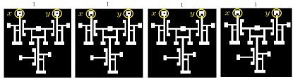
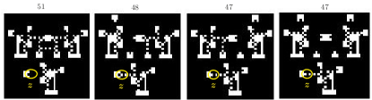
Figure 4: OR gate. The upper row shows the initial grid for the four input combinations, from left to right $(0,0)$, $(1,0)$, $(0,1)$, and $(1,1)$. The respective final grid for each input is shown in the lower row. The grid size is $40\times 40$.

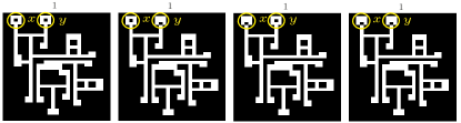
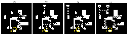
Figure 5: XOR gate. The upper row shows the initial grid for the four input combinations, from left to right $(0,0)$, $(0,1)$, $(1,0)$, and $(1,1)$. The respective final grid for each input is shown in the lower row. The grid size is $37\times 30$.

V Gliders and other computations

Not only binary logic but also trinary logic can be simulated using the underlying automaton. Consider the following trinary 2-input-2-output gate. Its inputs $x$ and $y$ each may take the values $0$, $1$ or $2$. One of its outputs $z$ is given by $x\triangleright y:=(2y-x)\mod 3$, and the other one is equal $y$, where $\mod$ denotes the modulo operation. Thus, if the two inputs are not the same then $z$ is different from both of them, and if the two inputs are the same then $x$, $y$, and $z$ all are equal.

The operation $\triangleright$ together with the set $Q=\{0,1,2\}$ induce a quandle algebra [13, 14]. Consider a set $Q$ together with a set $B$ of binary operations from $Q\times Q$ to $Q$ with the following properties:

1. $x\triangleright x=x$ for all $x\in Q$ and for all $\triangleright\in B$;

2. $(x\triangleright y)\triangleleft y=x$ for all $x,y\in Q$ and for all $\triangleright,~{}\triangleleft\in B$;

3. $(x\triangleright y)\triangleright z=(x\triangleright z)\triangleright(y\triangleright z)$ for all $x,y,z\in Q$ and for all $\triangleright\in B$.

We call the pair $(Q,B)$ satisfying the above properties a $B$- family of quandles or just a quandle. The above gate satisfies all the axioms of a quandle, where in this particular case the operations $\triangleright$ and $\triangleleft$ coincide.

In low-dimensional topology any quandle axiom corresponds to one Reidemeister move. A sequence of Reidemeister moves relate any two planar diagrams of the same knot or a tangle. When these tangle diagrams are colored by pieces of information they act much like circuits. Here, the instance of a line cutting through another line, known as a crossing, is seen as a 2-input-2-output gate whose operation is $\triangleright$. As shown in [13, 14] the quandle axioms may then be interpreted as laws of conservation of information. Indeed, the gates themselves are reversible and their inputs can be uniquely recovered from the respective outputs.

In the underlying automaton the additional value “2” is represented as “1” with a phase-shift. See Figure 6. The realization of the 2-input-2-output crossing gate is shown for the nine different input combinations in Figures 7, 8, and 9. As before, the upper row in each picture shows the grid at the beginning and the lower row shows its state after a number of iterations of the automaton rule.

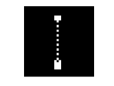
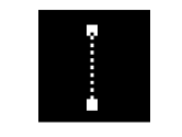
Figure 6: A wire carrying “1” (right) and a wire carrying “2” (left).

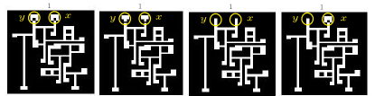
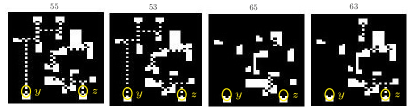
Figure 7: A 2-input-2-output trinary logic gate. From left to right the inputs are $(1,1)$, $(2,2)$, $(0,0)$, and $(0,1)$. The grid size is $43\times 34$.

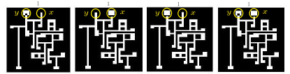
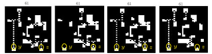
Figure 8: A 2-input-2-output trinary logic gate. From left to right the inputs are $(1,0)$, $(0,2)$, $(2,0)$, and $(1,2)$. The grid size is $43\times 34$.

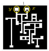
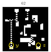
Figure 9: A 2-input-2-output trinary logic gate whose inputs are $(2,1)$. The grid size is $43\times 34$.

Gliders

Gliders are animated entities that emerge in the grid during the automaton evolution. In terms of computation such patterns are instrumental for carrying information across the grid. The Life-based Turing machine, for example, heavily relies on gliders to realize its logic and memory parts [21].

For reasons mentioned in the introduction, we suspect that the preceding cellular automaton cannot produce gliders. We were able, however, to generate gliders with an automaton whose rule permits at times the increase of a cell’s Kolmogorov complexity. One cycle of this automaton is as follows. In the beginning of a cycle it employs two rules to obtain the grid in the next time step:

Rule: Nothing comes out of nothing – do nothing to a (blank) cell whose Moore neighborhood vanishes.

Rule: A cell’s value is changed from $c$ to $1-c$ if the Kolmogorov complexity of its present Moore neighborhood is larger with $1-c$ than with $c$.

A single cycle of this automaton starts with a single iteration of Algorithm 2. For the next few time steps the automaton operates as described in Algorithm 1, i.e. it employs the “nowhere increasing” complexity rule. It proceeds so until the pair of grids, the recent one at an odd time step and the one two time steps back, are the same. This cycle is repeated indefinitely. A pseudocode for this automaton is given in Algorithm 3.

Algorithm 2 Nowhere decreasing Kolmogorov complexity CA

  Syntax: $c_{ij}(t+1)=\text{\bf CA}\uparrow(c_{ij}(t))$

  Input: $c_{ij}(t)$, $i=1,\ldots,N$, $j=1,\ldots,M$ (grid at time $t$)

  Output: $c_{ij}(t+1)$, $i=1,\ldots,N$, $j=1,\ldots,M$ (grid at time $t+1$)

  for $i=2:N-1$ do

     for $j=2:M-1$ do

        Let $A$ be the Moore neighborhood of $c_{ij}(t)$.

        if $A$ does not zeros then

           Obtain $K_{ij}(t)$ using $A$ from the lookup table [20].

           Flip the value of the middle cell in $A$ and similarly obtain $K^{\prime}_{ij}(t)$.

           if $K_{ij}(t)\geq K^{\prime}_{ij}(t)$ then

              $c_{ij}(t+1)=c_{ij}(t)$

           else

              $c_{ij}(t+1)=1-c_{ij}(t)$

           end if

        end if

     end for

  end for

Algorithm 3 Alternating, nowhere decreasing - nowhere increasing, CA

  Syntax: $c_{ij}(s)=\text{\bf CA}\updownarrow(c_{ij}(t))$

  Input: $c_{ij}(t)$, $i=1,\ldots,N$, $j=1,\ldots,M$ (grid at time $t$)

  Output: $c_{ij}(s)$, $i=1,\ldots,N$, $j=1,\ldots,M$ (grid at time $s$)

  $c_{ij}(t+1)=\text{\bf CA}\uparrow(c_{ij}(t))$

  $s=t+1$

  while $\{\exists i,j\;\;c_{ij}(s)\neq c_{ij}(s-2)\}\vee\{s\text{ is even}\}$ do

     $c_{ij}(s+1)=\text{\bf CA}\downarrow(c_{ij}(s))$

     $s=s+1$

  end while

The basic construction of a glider and its evolution in the course of two cycles of this automaton is shown in Figure 10.

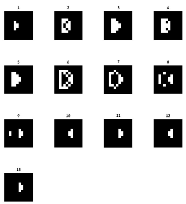
Figure 10: A two-cycle evolution of a glider using the cellular automaton in Algorithm 3. The first cycle starts with the grid numbered 1 and concludes with the grid numbered 5. The second cycle starts with grid 5 and concludes with grid 13. The grid size is $12\times 12$.

VI Grid’s average complexity

As neighborhoods overlap the average Kolmogorov complexity in the grid may increase even in “nowhere increasing” mode. The average Kolmogorov complexity of an $N\times M$ grid at time $t$ is defined as

$$\bar{K}(t)=(N-2)^{-1}(M-2)^{-1}\sum_{i=2}^{N-1}\sum_{j=2}^{M-1}K_{ij}(t).$$ (3)

When evaluating this measure for the NOT gate in Figure 2 the behavior in Figure 11 is observed. The transition from the initial to the final grid, in which complexity is lower on the average, shows instances where the average complexity rises.

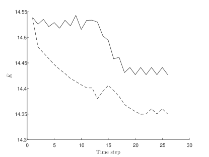
Figure 11: The average Kolmogorov complexity during the evolution of the NOT gate in Figure 2. The solid and dashed lines correspond, respectively, to the inputs $1$ and $0$.

Evaluating this measure for the automaton in Algorithm 2 results in the typical behavior shown in Figure 12. As one expects, its average complexity in Figure 13 tends to increase in time.

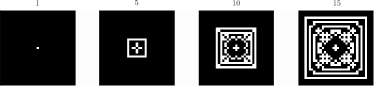
Figure 12: Expanding behavior of one source using the cellular automaton in Algorithm 2. The grid size is $30\times 30$.

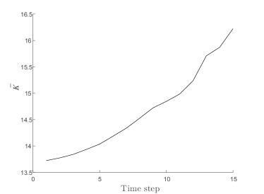
Figure 13: The average Kolmogorov complexity during the evolution of the the automaton in Figure 12.

VII Conclusion

This work is an attempt to address the questions raised in the beginning of this paper. The answer we offer is only partial. One may wonder whether any computable function can be computed by a similar “nowhere increasing” cellular automaton, or in other words, whether such an automaton is Turing-complete. For one reason we think it isn’t. During its evolution the initial grid on which the logical gate is encoded self-destructs. Therefore, outputs cannot be reused as inputs to the same logical gate. Although not proven, we suspect that this behavior hinders the construction of a memory device and thus also of a Turing-equivalent model of computation.

But the concept of using a measure of complexity to evolve is multifaceted. We have shown that a cellular automaton whose rule permits at times the increase of the cell’s neighborhood complexity can produce gliders. The lesson learned from Life is that gliders may become the basic ingredients in any computation and so perhaps this automaton also is Turing-complete.

As a final remark, we have used a particular measure of complexity. Other measures may similarly be used to evolve cellular automatons with different computational capabilities and behavior.

References

- [1]
- [2] J. von Neumann, “Theory of self-reproducing automata, univ. of ill,” Press, Urbana, Ill, 1966.
- [3] S. Wolfram, A New Kind of Science. Wolfram Media, 2002. [Online]. Available: http://www.wolframscience.com
- [4] K. Zuse, “Rechnender raum (calculating space),” 1969. [Online]. Available: http://www.mathrix.org/zenil/ZuseCalculatingSpace-GermanZenil.pdf
- [5] M. Cook, “Universality in elementary cellular automata,” Complex systems, vol. 15, no. 1, pp. 1–40, 2004.
- [6] E. Codd, “Cellular automata academic,” New York and London, 1968.
- [7] C. G. Langton, “Self-reproduction in cellular automata,” Physica D: Nonlinear Phenomena, vol. 10, no. 1-2, pp. 135–144, 1984.
- [8] J. Byl, “Self-reproduction in small cellular automata,” Physica D: Nonlinear Phenomena, vol. 34, no. 1-2, pp. 295–299, 1989.
- [9] J. Reggia, S. Armentrout, H. Chou, and Y. Peng, “Simple systems exhibiting self-directed replication,” Science, vol. 259, no. 26, pp. 1282–1287, 1993.
- [10] K. Lindgren and M. G. Nordahl, “Universal computation in simple one-dimensional cellular automata,” Complex Systems, vol. 4, no. 3, pp. 299–318, 1990.
- [11] N. Margolus, “Physics-like models of computation,” Physica D: Nonlinear Phenomena, vol. 10, no. 1-2, pp. 81–95, 1984.
- [12] P. Di Lena and L. Margara, “Computational complexity of dynamical systems: the case of cellular automata,” Information and Computation, vol. 206, no. 9-10, pp. 1104–1116, 2008.
- [13] A. Y. Carmi and D. Moskovich, “Computing with colored tangles,” Symmetry, vol. 7, no. 3, pp. 1289–1332, 2015.
- [14] D. Moskovich and A. Y. Carmi, “Tangle machines,” in Proc. R. Soc. A, vol. 471, no. 2179. The Royal Society, 2015, pp. 1–23.
- [15] J. T. Lizier, M. Prokopenko, and A. Y. Zomaya, “Local information transfer as a spatiotemporal filter for complex systems,” Physical Review E, vol. 77, no. 2, p. 026110, 2008.
- [16] A. N. Kolmogorov, “Three approaches to the quantitative definition ofinformation’,” Problems of information transmission, vol. 1, no. 1, pp. 1–7, 1965.
- [17] G. J. Chaitin, “On the length of programs for computing finite binary sequences: statistical considerations,” Journal of the ACM (JACM), vol. 16, no. 1, pp. 145–159, 1969.
- [18] E. Rivals, M. Dauchet, J.-P. Delahaye, and O. Delgrange, “Compression and genetic sequence analysis,” Biochimie, vol. 78, no. 5, pp. 315–322, 1996.
- [19] J.-P. Delahaye and H. Zenil, “Numerical evaluation of algorithmic complexity for short strings: A glance into the innermost structure of randomness,” Applied Mathematics and Computation, vol. 219, no. 1, pp. 63–77, 2012.
- [20] H. Zenil, F. Soler-Toscano, J.-P. Delahaye, and N. Gauvrit, “Two-dimensional kolmogorov complexity and an empirical validation of the coding theorem method by compressibility,” PeerJ Computer Science, vol. 1, pp. 1–31, 2015.
- [21] P. Rendell, “Game of life turing machine,” in Turing Machine Universality of the Game of Life. Springer, 2016, pp. 45–70.