Bayesian estimation of thermonuclear reaction rates for deuterium+deuterium reactions

Abstract

The study of d+d reactions is of major interest since their reaction rates affect the predicted abundances of D, ³He, and ⁷Li. In particular, recent measurements of primordial D/H ratios call for reduced uncertainties in the theoretical abundances predicted by big bang nucleosynthesis (BBN). Different authors have studied reactions involved in BBN by incorporating new experimental data and a careful treatment of systematic and probabilistic uncertainties. To analyze the experimental data, Coc et al. (2015) used results of ab initio models for the theoretical calculation of the energy dependence of S-factors in conjunction with traditional statistical methods based on $\chi^{2}$ minimization. Bayesian methods have now spread to many scientific fields and provide numerous advantages in data analysis. Astrophysical S-factors and reaction rates using Bayesian statistics were calculated by Iliadis et al. (2016). Here we present a similar analysis for two d+d reactions, d(d,n)³He and d(d,p)³H, that has been translated into a total decrease of the predicted D/H value by 0.16%.

1 Introduction

Big bang nucleosynthesis (BBN) is responsible for the formation of primordial ²H, ³He, ⁴He and ⁷Li. Considering that the primordial abundances of these isotopes span more than eight orders of magnitude, there is a fair agreement between BBN predictions and observations (see Cyburt et al. (2016) for a recent review). In recent years the uncertainties have been greatly reduced on both the primordial abundances deduced from observations, and on the parameters entering into the BBN model. For instance, observations of the anisotropies of the cosmic microwave background (CMB), e.g. by the Planck space mission (Ade et al., 2016), led to precise estimations of cosmological parameters. In particular, the baryonic density of the Universe was measured with an uncertainty of less than 1%: $\Omega_{\mathrm{b}}{\cdot}h^{2}$ = 0.02225$\pm$0.00016 (Ade et al., 2016). With this determination, the BBN model becomes parameter free and should be able to make accurate predictions.

However, it is now widely known (see Fields (2011) for a review) that there is a factor of three difference between the calculated ⁷Li/H ratio, by number of atoms (Cyburt et al., 2016; Coc et al., 2015), and the corresponding primordial value deduced from observations (Sbordone et al., 2010). The primitive lithium abundance is deduced from observations of low metallicity stars in the halo of our Galaxy, where the lithium abundance is almost independent of metallicity, displaying a plateau both as a function of metallicity and effective temperature. This puzzling discrepancy, known as the lithium problem, has not yet found a satisfactory solution (Coc, 2016) and casts a shadow on the model.

The uncertainty on the ⁴He primordial abundance, which is deduced from the observation of metal–poor extragalactic H II regions, has been reduced by the inclusion of an additional atomic infrared line in the analysis (Aver et al., 2015). For this isotope, BBN predictions agree well with observations, keeping in mind that these predictions rely on the n$\leftrightarrow$p weak reaction rates. One should note that these calculated rates incorporate various corrections that need to be assessed. The weak rates are also normalized to the experimental neutron lifetime whose recommended value, $\tau_{\rm{n}}$ = 880.3$\pm$1.1 s (Olive et al., 2014), has evolved in the last few years (Young et al., 2014).

Because of its low abundance, ³He, has not been observed outside of our Galaxy (Bania et al., 2002). Since it is both produced and destroyed in stars, its galactic chemical evolution is uncertain. It is, hence, presently of little use to constrain BBN. However, the next generation of 30+ m telescope facilities may allow to extract the ³He/⁴He ratio from observations of extra-galactic metal poor HII regions (Cooke, 2015).

Deuterium’s most primitive abundance is determined from the observation of few cosmological clouds at high redshift, on the line of sight of distant quasars. Up to a few years ago, there was a significant scatter in observations that lead to an $\approx$8% (Olive et al., 2012) uncertaininty on the primordial deuterium abundance. BBN prediction were, then, fully compatible with observations. However, recent measurements of primordial D/H, based on observations of damped Lyman-$\alpha$ systems at high redshift, led to an uncertainty of 1.3%, D/H = (2.547$\pm$0.033)$\times 10^{-5}$ (Cooke et al., 2014, 2016). This has to be compared to the most recent predictions of (2.45$\pm$0.05)$\times 10^{-5}$ (Coc et al., 2015) and (2.58$\pm$0.04)$\times 10^{-5}$ (Cyburt et al., 2016) that quote a 1.6–2.0% uncertainty, but whose central values differ by 5%. However, this difference almost vanishes if the same rates are used for the d(p,$\gamma)^{3}$He, d(d,n)³He and d(d,p)³H nuclear reactions (Tsung-Han Yeh, priv. comm.). These small, but significant, differences between obeservations and predictions require further investigations that are currently underway, in particular, the re-evaluations of reaction rates including the particle physics corrections to the weak rates, the comparison between numerical methods used in the network calculations and the comparison with other independent BBN codes and networks (e.g. Cyburt et al. (2016)). This paper concerns one important contribution to this goal, but others are needed before one is able to provide improved BBN predictions. This is why we will, here, only discuss relative effects of these new rates.

An improved D/H predicion is also very important for the lithium problem since most proposed solutions lead to an unacceptable increase of the deuterium abundance (Olive et al., 2012; Kusakabe et al., 2014; Coc et al., 2015). Indeed, for the CMB deduced baryonic density, ⁷Li is produced, during primordial nucleosynthesis, indirectly by ³He($\alpha,\gamma)^{7}$Be, where ⁷Be will decay much later to ⁷Li, while ⁷Be is destroyed by ⁷Be(n,p)⁷Li(p,$\alpha)^{4}$He. The solutions to the lithium problem generally rely on an increased late time neutron abundance to boost ⁷Be destruction through the ⁷Be(n,p)⁷Li(p,$\alpha)^{4}$He channel. These extra neutrons, inevitably, also boost the deuterium production through the ¹H(n,$\gamma)^{2}$H channel.

Hence, it is very important that the uncertainties on D/H predictions be reduced, because ($i$) the observational uncertainties of the primordial D/H ratio are smaller than those predicted by simulations, ($ii$) differences appear between predictions using different prescriptions for the reaction rates, and ($iii$) deuterium provides strong constraints to solutions of the lithium problem.

The precision of these calculations is currently limited by our knowledge of certain key thermonuclear reaction rates. For example, a 10% error in the d(p,$\gamma)^{3}$He, d(d,n)³He and d(d,p)³H rates causes a 3.2%, 5.4% and 4.6% uncertainty, respectively, in the predicted D/H ratio (Coc et al., 2015). The aim of our study is to reduce the uncertainties of BBN nucleosynthesis simulations as a continuation of our previous work that included the d(p,$\gamma)^{3}$He rate (Iliadis et al., 2016). Both d(d,n)³He and d(d,p)³H are non-resonant reactions, meaning that the S-factor, S(E), varies smoothly with energy. We apply a Bayesian analysis to the most recent experimental d+d S-factor data, and use the resulting improved S-factors to calculate the reaction rates. The theoretical model used for the S-factor (Arai et al., 2011) is assumed to accurately predict the energy dependence but not necessarily its absolute scale. The experimental data is used to scale this S-factor curve. We carry out a multiparametric estimation. The model parameters are the scale factor for the theoretical S-factor (we will refer to it as “overall scale factor” or “scale factor”) and a normalization factor for each data set accounting for systematic errors (we will refer to them as “normalization factors”). Hence, there is a total of 6 parameters for each reaction, since there is an overall scale factor and 5 normalization factors, one per data set. The Bayesian model provides a consistent description of all uncertainties involved (statistical and systematic), and yields the probability density for each parameter. Unlike traditional data analysis methods (e.g., Coc et al., 2015), it does not involve ad hoc assumptions or rely on Gaussian approximations for uncertainties. A more detailed explanation of this statistical analysis is given in Section 2. See Iliadis et al. (2016) for further information on these Bayesian models.

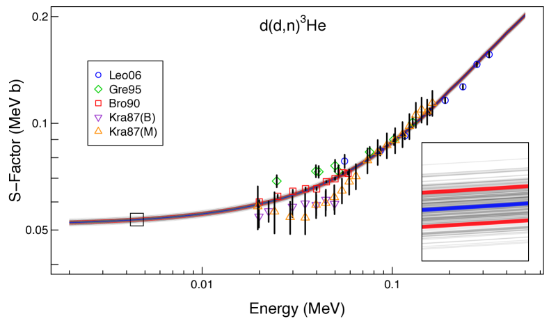
Figure 1: Astrophysical S-factor versus center-of-mass energy for the d(d,n)³He reaction. The symbols show the data of Leonard et al. (2006) (circles), Greife et al. (1995) (diamonds), Brown et al. (1990) (squares), Krauss et al. (1987) (B) (down-pointing triangles) and Krauss et al. (1987) (M) (up-pointing triangles). The error bars (1$\sigma$) refer to statistical uncertainties only. Grey lines forming the shaded area correspond to credible S-factors that result from different sets of parameter samples (the inset shows a magnification for a clearer view of these lines). The blue line is the median (50th percentile) of all credible S-factors, and red lines correspond to the 16th and 84th percentiles. The credible lines are calculated from the theoretical S-factor of Arai et al. (2011), multiplied by a scale factor that is a parameter of the Bayesian model.

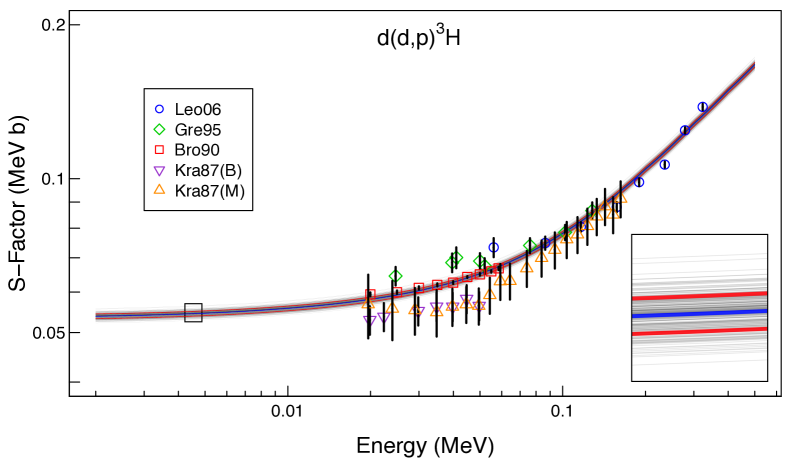
Figure 2: Astrophysical S-factor versus center-of-mass energy for the d(d,p)³H reaction. The symbols show the data of Leonard et al. (2006) (circles), Greife et al. (1995) (diamonds), Brown et al. (1990) (squares), Krauss et al. (1987) (B) (down-pointing triangles) and Krauss et al. (1987) (M) (up-pointing triangles). The error bars (1$\sigma$) refer to statistical uncertainties only. Grey lines forming the shaded area correspond to credible S-factors that result from different sets of parameter samples (the inset shows a magnification for a clearer view of these lines). The blue line is the median (50th percentile) of all credible S-factors, and red lines correspond to the 16th and 84th percentiles. The credible lines are calculated from the theoretical S-factor of Arai et al. (2011), multiplied by a scale factor that is a parameter of the Bayesian model.

2 Strategy: Bayesian statistics and MCMC

We adopt the ab initio calculation of Arai et al. (2011) for the energy-dependence of the S-factor. This microscopic calculation uses a four-nucleon configuration space with a realistic nucleon-nucleon interaction. Their study was focused on low energies only, where partial waves up to J=2 contribute to the reaction cross section. Therefore, their calculation underestimates the data above a center-of-mass energy of 1 MeV. Consequently, we took only data points below an energy of 0.6 MeV into account in our Bayesian model.

We analyzed S-factor data by means of Bayesian statistics and Markov chain Monte Carlo (MCMC) algorithms. We used the software JAGS (“Just Another Gibbs Sampler”) (Plummer, 2003), specifically the rjags package, withing the R language (R Core Team, 2015). The inputs for the program are the experimental data (Brown et al., 1990; Greife et al., 1995; Krauss et al., 1987; Leonard et al., 2006), the theoretical nuclear model we want to scale, and the prior distributions of the model parameters (i.e., the scale factor of the theoretical S-factor curve and the normalization factors of each data set). The way of constructing the Markov chain in this project is by a Metropolis-Hastings algorithm. Each step of the chain consists in a set of values for all six parameters (the overall scale factor and the normalization factors of five data sets). The transition from one step to another can be summarized as:

1. Given a state $\theta^{(i)}$, propose a new one $\theta^{\prime}$ by drawing a value from a proposal distribution (see Albert (2007)).

2. Accept the transition with a probability P$(\theta^{\prime}|\theta^{(i)})$=min$(1,$$\frac{\text{P}(\theta^{\prime}|S)}{\text{P}(\theta^{(i)}|S)})$, where $S$ stands for the experimental S-factor data. Moreover, P$(\theta|S)\propto$ P$(S|\theta)\cdot\pi(\theta)$, where P$(S|\theta)$ is the likelihood function and $\pi(\theta)$ is the prior distribution of the parameters. They are explained in Section 2.1.

3. If the transition is accepted, $\theta^{(i+1)}=\theta^{\prime}$. If not, $\theta^{(i+1)}=\theta^{(i)}$

4. Repeat 1-3.

When the Markov chain reaches the steady state, the values of the parameters taken at every step yield their posterior distributions. With that information, lately it was possible to estimate the reaction rates. For more information about this method, see the Appendices in Iliadis et al. (2016). As a general reference in this topic, see Hilbe (2017).

2.1 Likelihood and prior distributions

The likelihood distribution of the S-factor given a set of parameters and prior distributions of those parameters are needed to compute the acceptance probabilities in the Markov chain. The central limit theorem states that the probability density function resulting from the sum of independent random variables tends to a Gaussian distribution. By extension, a product of random variables will follow a lognormal distribution. Measured nuclear reaction cross sections and astrophysical S-factors result from the product (or ratios) of different physical quantities. Thus we can assume that the likelihood function for the S-factor (P$(S|\theta)$ in Section 2) will follow a lognormal distribution (Longland et al., 2010):

$$f(x)=\frac{1}{\sigma\sqrt{2\pi}x}e^{-(lnx-\mu)^{2}/(2\sigma^{2})},x>0$$ (1)

$\mu=\ln(E[x])-\dfrac{1}{2}\ln\bigg{(}1+\dfrac{V[x]}{E[x]^{2}}\bigg{)}$

$\sigma=\sqrt{\ln\bigg{(}1+\dfrac{V[x]}{E[x]^{2}}\bigg{)}}$

where $\mu$ is the location parameter for the normally distributed logarithm of random variable $x$, i.e., $e^{\mu}$ is the median of the distribution of $x$, and $\sigma$ is the spread parameter for the normally distributed logarithm of $x$; E[x] and V[x] denote the expected mean value and the variance, respectively, of the lognormal distribution. One advantage of this type of distribution is that negative S-factor values, which are unphysical, are not allowed. The lognormal likelihood function is then given by:

$$\text{P}(\text{{S}}|\text{{{f}}})=\prod_{i=1}^{N}\frac{1}{S_{i}\sqrt{2\pi\sigma_{L;i}^{2}}}\text{ exp}\Bigg{[}\frac{(\text{ln}\;S_{i}-\mu_{i})^{2}}{2\sigma_{L;i}^{2}}\Bigg{]}$$ (2a)

$$\mu_{i}=\text{ln}\;(f_{n}f_{s}S_{th})-\frac{1}{2}\text{ln}\;\big{(}1+\frac{\sigma_{i}^{2}}{(f_{n}f_{s}S_{th})^{2}}\big{)}$$ (2b)

$$\sigma_{L;i}^{2}=\text{ln}\big{(}1+\frac{\sigma_{i}^{2}}{(f_{n}f_{s}S_{th})^{2}}\big{)}$$ (2c)

where $S_{i}$ stands for the experimental S-factor data, f are the sampled parameters ($f_{n}$ is the normalization factor for a particular data set and $f_{s}$ is the overall scale factor), $N$ is the number of measurements of the data set, $\mu_{i}$ is the location parameter of data point $i$, $\sigma_{L;i}$ is the spread parameter of data point $i$, $S_{th}$ corresponds to the theoretical S-factor and $\sigma_{i}$ is the reported standard deviation of data point $i$. Notice that there is no degeneracy regarding the product $f_{n}\cdot f_{s}$, since $f_{n}$ is different for each data set while $f_{s}$ is the same parameter throughout.

Since the scale factor, $f_{s}$, is expected to be close to unity, we assume for the overall scaling factor a non-informative prior ($\pi(\theta)$ in Section 2), i.e., a normally distributed probability density with a mean of zero and a standard deviation of 100. Therefore we expressed the prior for the scale factor as:

$$\pi(f_{s})=\begin{cases}\frac{1}{\sqrt{2\pi 100^{2}}}\text{exp}\Bigg{[}\frac{(f_{s}-0.0)^{2}}{2\cdot 100^{2}}\Bigg{]},&\text{for }f_{s}>0\\ 0&\text{for }f_{s}\leq 0\end{cases}$$ (3)

The distribution was truncated at zero since the scaling factor must be a positive quantity. To test the sensitivity of our results, we repeated the analysis using different priors (e.g., uniform distributions and gamma functions), and the results were very similar in all cases. For the normalization factors of each data set, we assumed highly informative priors. It is discussed in Section 2.2.

Additionally, we incorporate a robust regression method to avoid the bias that outliers can introduce in the results. Our algorithm accomplishes this by detecting possible outliers (i.e., measurements with over-optimistic uncertainties) and reducing their influence in the analysis (see Section 2.3).

2.2 Systematic uncertainties

A measurement is usually subject to statistical and systematic uncertainties. Statistical uncertainties are inherent to any physical process and cannot be avoided. They can be reduced by combining results from different measurements, leading to different measured values for the same experimental conditions. Conversely, systematic uncertainties will not change if the experimental conditions remain the same. Hence, all of the data points from the same measurement will likely be affected by a systematic effect in a similar manner. We introduce statistical uncertainties in our model by assuming lognormal priors for the individual normalization factors, $f_{n;k}$, of all five data sets, $k$.

The experimental data considered in this study (Brown et al., 1990; Greife et al., 1995; Krauss et al., 1987; Leonard et al., 2006) provided systematic uncertainties for each data set as normalization factor uncertainties 1+$\epsilon$, with $\epsilon$ given in Table II of Coc et al. (2015). We include in our Bayesian model a systematic effect as a highly informative, lognormal prior. The parameters of this distribution are a median of 1.0, i.e., $e^{\mu}$ $=$ $1$, and a systematic factor uncertainty of $e^{\sigma_{k}}$. This prior can be written as:

$$\pi(f_{n;k})=\frac{1}{f_{n;k}\sqrt{2\pi(\text{ln}(e^{\sigma_{k}}))^{2}}}\text{exp}\Bigg{[}\frac{(\text{ln}\;f_{n;k}-\text{ln}(1.0))^{2}}{2(\text{ln}(e^{\sigma_{k}}))^{2}}\Bigg{]}$$ (4)

For more information on this choice of prior, see Iliadis et al. (2016).

2.3 Robust regression

Outliers can bias the data analysis significantly and thus need to be treated carefully. In our JAGS code, we model outliers as data points with over-optimistic reported uncertainties. The algorithm designates each data point as either having believable uncertainty (i.e., not an outlier) or over-optimistic uncertainty (i.e., outlier). This operation is done for each step of the chain. Ultimately, data points having smaller outlier probabilities are more heavily weighted in the final results, thus reducing the statistical weight of the outliers (Andreon & Weaver, 2015). For the presentation of these results, we average the outlier probabilities for all data points in a given set and list the values in Tables 1 and 2.

3 Bayesian astrophysical S-factors

The astrophysical S-factor of a nuclear reaction is defined as:

$$S(E)\equiv\sigma(E)Ee^{2\pi\eta}$$ (5)

where $\sigma$(E) is the cross-section of the reaction at the center-of-mass energy E and $e^{2\pi\eta}$ is the Gamow factor, which depends on the charges of the projectile and the target, the relative atomic masses, and the energy E (see Iliadis (2015) for details).

The theoretical model used here for the energy dependence of the d+d S-factor is based on a multichannel ab initio calculation (Arai et al., 2011). We assume that the nuclear model accurately predicts the energy dependence of the S-factor, but not necessarily its absolute scale. Our model predicts the best estimate of the overall scale factor and its uncertainty.

The Bayesian model for the analysis of the S-factor has several parameters. These include the normalization factors for each of the five individual data sets as well as the overall scale factor of the theoretical S-factor curve.

We employ the same procedure as Iliadis et al. (2016), and we use three different Markov chains of 7500 steps each, with a burn-in of 2000 steps. These values ensure the convergence of the chains and that the Monte Carlo fluctuations are negligible compared to the statistical and systematic uncertainties. We performed several tests with different chain lengths (e.g., 75000 steps) and the results were the same.

Figure 3: Results for d(d,n)³He. (Top) Overall scale factor for the theoretical S-factor. (Bottom) Normalization factors of each data set: Leonard et al. (2006) (Leo06), Greife et al. (1995) (Gre95), Brown et al. (1990) (Bro90), Krauss et al. (1987) (Kra87 (B) and Kra87 (M)). Present and previous (Coc et al., 2015) results are shown in red and black, respectively. The range indicated in red corresponds to the 68% credible interval of the posterior. The range indicated in black shows the 68% confidence interval of the traditional analysis.

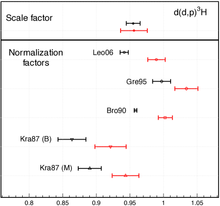
Figure 4: Results for d(d,p)³H. (Top) Overall scale factor for the theoretical S-factor. (Bottom) Normalization factors of each data set: Leonard et al. (2006) (Leo06), Greife et al. (1995) (Gre95), Brown et al. (1990) (Bro90), Krauss et al. (1987) (Kra87 (B) and Kra87 (M)). Present and previous (Coc et al., 2015) results are shown in red and black, respectively. The range indicated in red corresponds to the 68% credible interval of the posterior. The range indicated in black shows the 68% confidence interval of the traditional analysis.

3.1 Results

Traditional methods based on $\chi^{2}$ minimization have been applied to the calculation of the d+d reaction rates by Coc et al. (2015). In their analysis, they assumed that the scale factor is given by the weighted average of the normalization factors that independently fit each data set to the theoretical S(E) curve. They made a number of ad hoc assumptions to include systematic errors in their analysis and assumed Gaussian approximations for the uncertainties (see Appendix A in Coc et al. (2015)). Their results were deemed satisfactory by the authors, since the reduced $\chi^{2}$ was always close to unity.

Bayesian S-factors are shown in Figure 1 for d(d,n)³He and Figure 2 for d(d,p)³H. Grey lines represent credible S-factor curves for different sets of parameters, yielding the shaded region. All of the credible S-factors are close to the median value (blue line). The red lines correspond to the 16th and 84th percentiles.

Results from our Bayesian analysis, and the traditional method (Coc et al., 2015) for comparison, are shown in Tables 1 and 2 for the d(d,n)³He and d(d,p)³H reactions, respectively. Some of the results are also displayed in Figures 3 and 4, where the red data points correspond to the present Bayesian method and the black data points correspond to the traditional $\chi^{2}$ minimization. The top panels (labeled as “Scale factor”) display the overall scale factor. For both reactions, the scale factors are in agreement. It can also be seen that the scale factors are smaller than unity (see Tables 1 and 2), i.e., the theoretical S-factor curve exceeds the data. The bottom regions (labeled as “Normalization factors”) of Figures 3 and 4 show the normalization factors of each data set. It can be seen that the Bayesian normalization factors are consistently larger than the traditional analysis values. This is caused by the different methods to calculate these factors, as explained below.

In the Bayesian approach, the theoretical S-factor is multiplied by the overall scale factor. We defined our Bayesian model so that each data set is the result of multiplying the scaled S-factor curve by a normalization factor. As explained before, this normalization factor includes the effect of systematic uncertainties. Hence, at each step of the Markov chain, there is a shift in the magnitude of the theory (scaling) and the data sets (to account for the systematic uncertainties). These shifts are performed by multiplying the S-factor theoretical curve by the overall scale factor and dividing each data set by its corresponding normalization factor. Each measurement is affected by a multiplicative error ($S_{exp}=f_{n}\cdot S_{true}$, where $S_{exp}$ is the experimental datum, $f_{n}$ is the normalization factor and $S_{true}$ is the actual value), so we must divide the experimental value by the normalization factor if we want to cancel it. In this way, the final probability density function for each parameter is influenced by all other parameters.

In the traditional analysis performed by Coc et al. (2015), however, the theoretical S-factor is multiplied by a normalization factor for each data set separately. The overall scale factor is then obtained by computing the weighted average of all normalization factors. The systematic uncertainties are introduced in the weights of the average by adding systematic and statistical errors quadratically for each data set (see Eq. (A8) in Coc et al. (2015)).

To explain the discrepancies between traditional and Bayesian normalization factors, consider the data presented in Figure 5. This figure shows the measured d(d,n)³He S-factors of each data set. The solid curve shows the ab initio S-factor of Arai et al. (2011) before scaling. At each step of the Markov chain, the Bayesian model suggests a new value smaller than unity for the overall scale factor, to displace the curve downwards. The model also samples a new normalization factor for each data set. As an example, look at the suggested normalization factor for Kra (B) in Table 1 (0.922$\pm$0.024). It is less than unity since these experimental points should be shifted upwards to correct the effect of the systematic errors. Moreover, each normalization factor is influenced by the overall scale factor: at each step, the normalization factor fits the data to the scaled theory. In the traditional analysis, each normalization factor is calculated independently to fit the original S-factor. In the case of Kra (B), the traditional normalization factor needs to perform a larger shift, i.e. it will be further away from unity. This means a smaller normalization factor in the traditional case than in the Bayesian one.

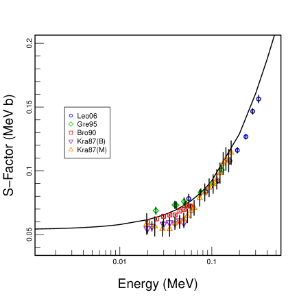
Figure 5: Astrophysical S-factor versus center-of-mass energy for d(d,n)³He. Experimental points are from (Leonard et al., 2006), (Greife et al., 1995), (Brown et al., 1990), and (Krauss et al., 1987). The error bars (1$\sigma$) refer to statistical uncertainties only. The solid curve shows the ab initio S-factor of Arai et al. (2011) before scaling.

Table 1: Results for the d(d,n)³He reaction.

Data		Present		Previous
Ref.	n	norm	outlier	norm	$\chi^{2}_{\nu}$
Leo 06	8	$0.978_{-0.011}^{+0.012}$	55.1%	$0.933\pm 0.007$	2.033
Gre 95	8	$1.045_{-0.017}^{+0.017}$	45.4%	$1.016\pm 0.013$	1.247
Bro 90	9	$1.004_{-0.010}^{+0.010}$	64.6%	$0.964\pm 0.003$	2.366
Kra 87 (B)	7	$0.922_{-0.024}^{+0.024}$	35.3%	$0.868\pm 0.022$	0.292
Kra 87 (M)	20	$0.964_{-0.021}^{+0.021}$	27.6%	$0.919\pm 0.018$	0.624
Quantity		Present		Previous
Scale factor:		$0.961_{-0.010}^{+0.010}$		$0.959\pm 0.010$ $(\chi^{2}_{\nu}=1.33)$
S(0) (keVb):		$51.70_{-0.51}^{+0.54}$		-

Table 2: Results for the d(d,p)³H reaction.

Data		Present		Previous
Ref.	n	norm	outlier	norm	$\chi^{2}_{\nu}$
Leo 06	8	$0.989_{-0.013}^{+0.013}$	80.4%	$0.942\pm 0.006$	5.376
Gre 95	8	$1.034_{-0.017}^{+0.017}$	30.6%	$0.997\pm 0.013$	0.999
Bro 90	9	$1.002_{-0.010}^{+0.011}$	51.9%	$0.958\pm 0.002$	1.969
Kra 87 (B)	7	$0.921_{-0.023}^{+0.023}$	21.1%	$0.864\pm 0.021$	0.100
Kra 87 (M)	20	$0.944_{-0.020}^{+0.020}$	8.6%	$0.890\pm 0.017$	0.177
Quantity		Present		Previous
Scale factor:		$0.956_{-0.011}^{+0.010}$		$0.955\pm 0.010$ $(\chi^{2}_{\nu}=1.33)$
S(0) (keVb):		$53.26_{-0.59}^{+0.55}$		-

4 Reaction rates

The thermonuclear reaction rate per particle pair, $N_{A}\left\langle\sigma v\right\rangle$, can be written as:

$$\begin{split}N_{A}\left\langle\sigma v\right\rangle=&\bigg{(}\frac{8}{\pi m_{01}}\bigg{)}^{1/2}\frac{N_{A}}{(kT)^{3/2}}\\ &\int_{0}^{\infty}e^{-2\pi\eta}S(E)e^{-E/kT}dE\end{split}$$ (6)

where $m_{01}$ is the reduced mass of projectile and target, $N_{A}$ represents Avogadro’s constant, and the product of Boltzmann constant, $k$, and plasma temperature, $T$, is given by

$$kT=0.086173324\>T_{9}\text{ (MeV)}$$ (7)

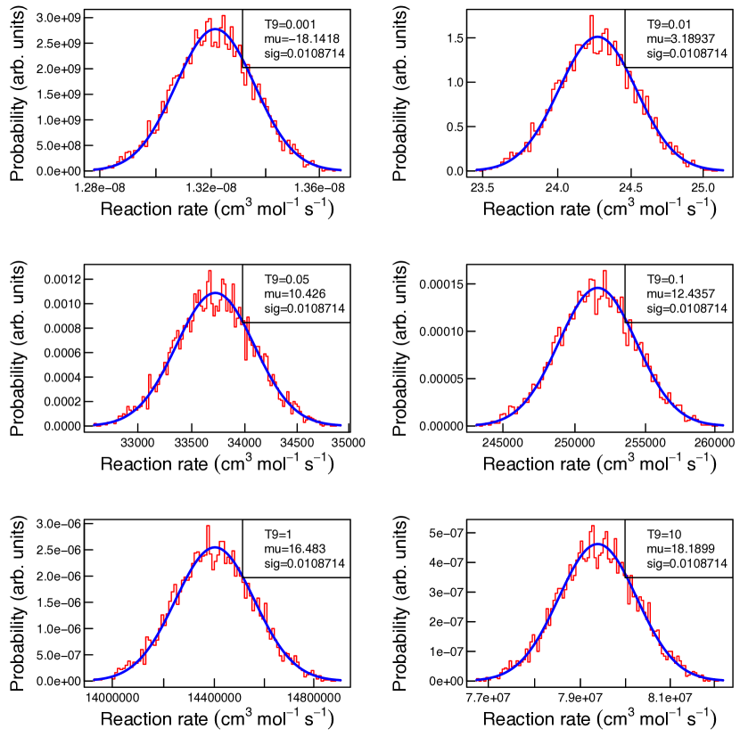
Figure 6: Reaction rate probability density of d(d,n)³He at different temperatures. The rate samples (red histograms) are computed using the S-factor samples obtained from the Bayesian analysis. Blue curves represent lognormal approximations, where the lognormal parameters $\mu$ (‘mu”) and $\sigma$ (“sig”) are directly calculated from the expectation value and variance of all rate samples, ln($N_{A}\left\langle\sigma v\right\rangle_{i}$), at a given temperature. T9 is the temperature in GK.

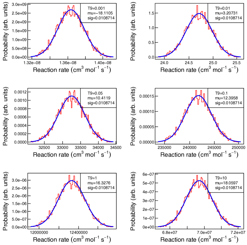
Figure 7: Reaction rate probability density of d(d,p)³H at different temperatures. The rate samples (red histograms) are computed using the S-factor samples obtained from the Bayesian analysis. Blue curves represent lognormal approximations, where the lognormal parameters $\mu$ (‘mu”) and $\sigma$ (“sig”) are directly calculated from the expectation value and variance of all rate samples, ln($N_{A}\left\langle\sigma v\right\rangle_{i}$), at a given temperature. T9 is the temperature in GK.

with the temperature, $T_{9}$, in units of GK (see Iliadis (2015) for details). The reaction rates are calculated by numerical integration of Eq. (6) for each set of parameters sampled by the Markov chain, at 60 different temperatures between 1 MK and 10 GK. The reaction rate probability densities at selected temperatures are shown in Figures 6 and 7 in red. The blue lines correspond to a lognormal approximation (Longland et al., 2010), for convenient implementation of the rates in libraries such as STARLIB (Sallaska et al., 2013). Numerical reaction rate values are listed in Table 3. The recommended rates are computed as the 50th percentile of the probability density, while the rate factor uncertainty, f.u., is obtained from the 16th and 84th percentiles. The lognormal parameters, $\mu$ and $\sigma$, can be calculated from the recommended (median) rate ($x_{med}=e^{\mu}$) and the factor uncertainty ($f.u.=e^{\sigma}$; for a coverage probability of 68%). The rate factor uncertainty is 1.1% for both reactions at most temperatures.

The present rates for d(d,n)³He and d(d,p)³H agree with the results of Coc et al. (2015) within 1% at most temperatures. However, our rates are more than 15% larger than those of Coc et al. (2015) at very low temperatures (near 1 MK). This is caused by a low-energy cutoff that is too high for the numerical integration of the rates in the previous analysis. The theoretical model of Arai et al. (2011) only applies to low energies, and thus we can derive Bayesian reaction rates only up to a temperature of 2 GK. The results in Table 3 for higher temperatures, shown in italics, are adopted from Coc et al. (2015). The most important temperatures for BBN are near 1 GK, corresponding to an effective kinetic energy range of $<$250 keV for the d+d reactions.

The last step is to calculate the effect of the new reaction rates on the predicted primordial D/H ratio. The Bayesian mean value for the scale factor is larger by 0.21% for d(d,n)³He and larger by 0.12% for d(d,p)³H compared to Coc et al. (2015). The discrepancies of both reaction rates (0.21% and 0.12%, respectively), weighted by the sensitivity of the D/H abundance ratio to each reaction rate variation (-0.54 and -0.46, respectively) (Coc et al., 2010), result in a 0.113% and 0.055% decrease of the central D/H value. Fortuitously, the uncertainties on the scale factors (see Tables 1 and 2) are almost identical to the former ones (Coc et al., 2015). Hence, when using these two new reaction rates, instead of the Coc et al. (2015) ones, this translates to a 0.16% decrease of the predicted D/H value, while its total uncertainty remains unchanged at 2.0%. Half of this error budget originates from the d(p,$\gamma$) reaction rate and it would be premature to update the D/H value before new measurements concerning this reaction, done at LUNA, are published (see Mossa (2017)). Only after these new data are made available and the investigation of other sources of uncertainties (numerical, correction to weak rates,…) are completed, it will be relevant to provide new predictions of D/H.

Table 3: Present recommended reaction rates.

	d(d,n)3He		d(d,p)3H
T (GK)	Rate	$f.u.$	Rate	$f.u.$
0.001	1.322E-08	1.011	1.364E-08	1.011
0.002	5.489E-05	1.011	5.653E-05	1.011
0.003	3.025E-03	1.011	3.110E-03	1.011
0.004	3.737E-02	1.011	3.835E-02	1.011
0.005	2.214E-01	1.011	2.269E-01	1.011
0.006	8.556E-01	1.011	8.755E-01	1.011
0.007	2.508E+00	1.011	2.563E+00	1.011
0.008	6.074E+00	1.011	6.198E+00	1.011
0.009	1.280E+01	1.011	1.304E+01	1.011
0.010	2.427E+01	1.011	2.471E+01	1.011
0.011	4.242E+01	1.011	4.314E+01	1.011
0.012	6.945E+01	1.011	7.055E+01	1.011
0.013	1.078E+02	1.011	1.094E+02	1.011
0.014	1.602E+02	1.011	1.624E+02	1.011
0.015	2.293E+02	1.011	2.322E+02	1.011
0.016	3.183E+02	1.011	3.220E+02	1.011
0.018	5.674E+02	1.011	5.729E+02	1.011
0.020	9.321E+02	1.011	9.395E+02	1.011
0.025	2.507E+03	1.011	2.516E+03	1.011
0.030	5.307E+03	1.011	5.305E+03	1.011
0.040	1.570E+04	1.011	1.558E+04	1.011
0.050	3.373E+04	1.011	3.325E+04	1.011
0.060	6.020E+04	1.011	5.900E+04	1.011
0.070	9.539E+04	1.011	9.298E+04	1.011
0.080	1.392E+05	1.011	1.350E+05	1.011
0.090	1.914E+05	1.011	1.847E+05	1.011
0.100	2.516E+05	1.011	2.418E+05	1.011
0.110	3.194E+05	1.011	3.056E+05	1.011
0.120	3.943E+05	1.011	3.758E+05	1.011
0.130	4.759E+05	1.011	4.518E+05	1.011
0.140	5.638E+05	1.011	5.334E+05	1.011
0.150	6.575E+05	1.011	6.199E+05	1.011
0.160	7.568E+05	1.011	7.111E+05	1.011
0.180	9.702E+05	1.011	9.061E+05	1.011
0.200	1.201E+06	1.011	1.116E+06	1.011
0.250	1.843E+06	1.011	1.691E+06	1.011
0.300	2.555E+06	1.011	2.321E+06	1.011
0.350	3.318E+06	1.011	2.988E+06	1.011
0.400	4.118E+06	1.011	3.681E+06	1.011
0.450	4.944E+06	1.011	4.391E+06	1.011
0.500	5.788E+06	1.011	5.113E+06	1.011
0.600	7.510E+06	1.011	6.573E+06	1.011
0.700	9.251E+06	1.011	8.036E+06	1.011
0.800	1.099E+07	1.011	9.489E+06	1.011
0.900	1.271E+07	1.011	1.092E+07	1.011
1.000	1.440E+07	1.011	1.233E+07	1.011
1.250	1.850E+07	1.011	1.572E+07	1.011
1.500	2.236E+07	1.011	1.893E+07	1.011
1.750	2.599E+07	1.011	2.194E+07	1.011
2.000	2.938E+07	1.011	2.477E+07	1.011
2.500	3.546E+07	1.012	2.976E+07	1.013
3.000	4.093E+07	1.014	3.440E+07	1.014
3.500	4.585E+07	1.014	3.863E+07	1.014
4.000	5.031E+07	1.015	4.251E+07	1.015
5.000	5.816E+07	1.016	4.946E+07	1.016
6.000	6.488E+07	1.017	5.552E+07	1.017
7.000	7.072E+07	1.018	6.077E+07	1.018
8.000	7.583E+07	1.018	6.529E+07	1.018
9.000	8.037E+07	1.018	6.912E+07	1.018
10.000	8.437E+07	1.018	7.228E+07	1.019

Reaction rates in units of cm³mol^-1s^-1, corresponding to the 50th percentile of the rate probability density function. The rate factor uncertainty, f.u., is obtained from the 16th and 84th percentiles (see text). The parameters $\mu$ and $\sigma$ of the lognormal approximation to the reaction rate are given by $x_{med}=e^{\mu}$ and $f.u.=e^{\sigma}$, respectively, where $x_{med}$ denotes the median rate. Values for $T>2$ GK, shown in italics, are adopted from Coc et al. (2015).

5 Conclusions

We presented improved reaction rates for d(d,n)³He and d(d,p)³H based on the Bayesian method discussed in Iliadis et al. (2016). Unlike previous methods that were based on traditional statistics (i.e., $\chi^{2}$ minimization), our method does not rely on weighted averages or the quadratic addition of systematic and statistical errors. For both reactions, the rate factor uncertainty is 1.1% and agrees with the traditional results. However, the Bayesian scale factors by which the theory needs to be multiplied to fit the data are larger than those of Coc et al. (2015). We obtained scale factors which are 0.20% larger for d(d,n)³He and 0.12% larger for d(d,p)³H. This translates to a 0.16% decrease of the predicted D/H value, while its total uncertainty remains unchanged at 2.0%. This shows the robustness of the deuterium predictions, provided that the same experimental data and nuclear model are used. It leaves very little room for those solutions to the lithium problem that cannot avoid an increase in D/H. It also calls for improved theoretical calculations. The theoretical work of Arai et al. (2011), used here, was focused on low energies and does not correctly reproduce the experimental data above $\approx$600 keV. It is highly desirable that these calculations be extended up to $\approx$2 MeV, to cover the range of experimental data.

Here we presented the first statistically rigorous results for d+d reaction rate probability densities. These can be employed in future Monte Carlo studies of big bang nucleosynthesis.

6 Acknowledgements

We would like to thank Jordi José, Jack Dermigny, Rafa De Souza, Lori Downen and Sean Hunt for their support and feedback. One of us (AGI) would like to express his gratitude to the Department of Physics and Astronomy for hospitality during his visit to UNC-CH, where this project was started. This work was supported in part by NASA under the Astrophysics Theory Program grant 14-ATP14-0007 and the U.S. DOE under Contract No. DE-FG02-97ER41041.

References

- Ade et al. (2016) P. A. R. Ade et al. (Planck Collaboration XIII), 2016, Astron. & Astrophys., 594, A13
- Albert (2007) Albert, J. (2007), Bayesian computation with R, (1st Edition, New York, Springer)
- Andreon & Weaver (2015) Andreon, S., & Weaver, B. 2015, Bayesian Methods for the Physical Sciences, (Switzerland: Springer Inetrnational Publishing)
- Arai et al. (2011) Arai, K., Aoyama, S., Suzuki, Y., Descouvemont, P. & Baye, D. 2011, Phys. Rev. Lett. 107, 132502
- Aver et al. (2015) Aver, E., Olive, K.A. & Skillman, E.D., 2015, JCAP 07, 011
- Brown et al. (1990) Brown, R. E. & Jarmie, N. 1990, Phys. Rev. C 41, 1391
- Bania et al. (2002) Bania, T., Rood, R. & Balser, D., 2002, Nature, 415, 54
- Coc et al. (2010) Coc, A. & Vangioni, E. 2010, J. Phys. Conf. Ser. 202, 012001
- Coc et al. (2015) Coc, A., Petitjean, P., Uzan, J.-P., Vangioni, E., Descouvemont, P., Iliadis, C. & Longland, R. 2015, Phys. Rev. D, 92, 123526
- Coc (2016) Coc, A., 2017 in Proc. of the 14th International Symposium on Nuclei in the Cosmos (NIC2016), ed. JPS Conf. Proc. 14, 010102
- Cooke et al. (2014, 2016) Cooke, R. J., Pettini, M., Nollett, K. M., & Jorgenson, R. 2016, The Astrophysical Journal, 830(2), 148, 16pp
- Cooke (2015) Cooke, R. J. 2015, The Astrophysical Journal Letters, 812(1), L12, 5pp
- Cyburt et al. (2016) Cyburt, R. H., Fields, B. D., Olive, K. A., & Yeh, T. H. 2016, Reviews of Modern Physics, 88(1), 015004
- Descouvemont et al. (2004) Descouvemont, P., Adahchour, A., Angulo, C., Coc, A., & Vangioni-Flam, E. 2004, Atomic Data and Nuclear Data Tables, 88(1), 203-236
- Fields (2011) Fields, B.D., 2011, Annu. Rev. Nucl. Part. Sc., 6, 47
- Greife et al. (1995) Greife, U., Gorris, F., Junker, M., Rolfs, C. & Zahnow, D. 1995, Z. Phys. A 351, 107
- Hilbe (2017) Hilbe, J.M., de Souza, R.S. & Ishida, E.O. 2017, Bayesian Models for Astrophysical Data Using R, JAGS, Python, and Stan, (1st Edition, Cambridge University Press)
- Iliadis (2015) Iliadis, C. 2015, Nuclear Physics of Stars, (2nd Edition, Weinheim, Wiley-VCH)
- Iliadis et al. (2016) Iliadis, C., Anderson, K. S., Coc, A., Timmes, F. X. & Starrfield, S. 2016, The Astrophysical Journal, 831(1), 107
- Krauss et al. (1987) Krauss, A., Becker, H. W., Trautvetter, H. P., Rolfs, C. & Brand, K. 1987, Nucl. Phys. A465, 150
- Kusakabe et al. (2014) Kusakabe, M., Cheoun, M.–K., & Kim, K. S., 2014, Phys. Rev. D, 90, 045009
- Leonard et al. (2006) Leonard, D. S., Karwowski, H. J., Brune, C. R., Fisher, B. M. & Ludwig, E. J. 2006, Phys. Rev. C, 73, 045801
- Longland et al. (2010) Longland, R., Iliadis, C., Champagne, A. E., Newton, J. R., Ugalde, C., Coc, A. & Fitzgerald, R. 2010, Nucl. Phys. A, 841, 1
- Mossa (2017) Mossa, V. in proceedings of Nuclear Physics in Astrophysics 8, NPA8: 18-23 June 2017, Catania
- Olive et al. (2012) Olive, K.A., Petitjean, P., Vangioni, E., & Silk, J., 2012, MNRAS, 426, 1427
- Olive et al. (2014) Olive, K.A., et al. (Particle Data Group), 2014, Chin. Phys. C, 38, 090001
- Plummer (2003) Plummer, M. 2003, JAGS: A program for analysis of Bayesian graphical models using Gibbs sampling, in: Proceedings of the 3rd International Workshop on Distributed Statistical Computing (dsc 2003), Vienna, Austria, ISSN 1609-395X
- R Core Team (2015) R Core Team 2015, R: A language and environment for statistical computing, R Foundation for Statistical Computing, Vienna, Austria, (https://www.R-project.org/)
- Riemer-Sørensen (2017) Riemer-Sørrensen, S., Kotuš, S., Webb, J. K. , Ali, K., Dumont, V., Murphy, M.T., & Carswell, R. F. , 2017, MNRAS, 468, 3239
- Sallaska et al. (2013) Sallaska, A.L., Iliadis, C., Champagne, A. E., Goriely, S., Starrfield, S., & Timmes, F.X. 2013, Astrophys. J. Suppl. 207, 18
- Sbordone et al. (2010) Sbordone, Bonifacio, L., P., Caffau E., et al., 2010, A&A, 522, A26
- Young et al. (2014) Young, A.R., Clayton, S., Filippone, B.W., Geltenbort, P., Ito, T.M., et al., 2014, J. Phys. G: Nucl. Part. Phys., 41, 114007