Reduced Basis POD-Galerkin Method for Parametrized Optimal Control Problems in Environmental Marine Sciences and Engineering

Abstract

In this work we propose reduced order methods as a suitable approach to face parametrized optimal control problems governed by partial differential equations, with applications in environmental marine sciences and engineering. Environmental parametrized optimal control problems are usually studied for different configurations described by several physical and/or geometrical parameters representing different phenomena and structures. The solution of parametrized problems requires a demanding computational effort. In order to save computational time, we rely on reduced basis techniques as a suitable and rapid tool to solve parametrized problems. We introduce general parametrized linear quadratic optimal control problems, and the saddle-point structure of their optimality system. Then, we propose a POD-Galerkin reduction of the optimality system. We test the resulting method on two environmental applications: a pollutant control in the Gulf of Trieste, Italy and a solution tracking governed by quasi-geostrophic equations describing North Atlantic Ocean dynamic. The two experiments underline how reduced order methods are a reliable and convenient tool to manage several environmental optimal control problems, for different mathematical models, geographical scale as well as physical meaning. The quasi-geostrophic optimal control problem is also presented in its nonlinear version.

Keywords: reduced order methods, proper orthogonal decomposition, parametrized optimal control problems, PDEs state equations, environmental marine applications, quasi-geostrophic equation.

AMS: 49J20, 76N25, 35Q35

1 Introduction

Parametrized optimal control problems (OCP($\boldsymbol{\mu}$)s) governed by parametrized partial differential equations (PDE($\boldsymbol{\mu}$)s) are usually complex and demanding, computationally speaking. In this case the parameter $\boldsymbol{\mu}\in\mathcal{P}\subset\mathbb{R}^{d}$ could represent physical or geometrical features. In order to study different configurations, a rapid and suitable approach based on reduced order models could allow to face OCP($\boldsymbol{\mu}$)s in a low dimensional framework. Computational methods for OCP($\boldsymbol{\mu}$)s are a quite widespread tool in many contexts and fields: in shape optimization (see e.g. [20, 25, 35]), in flow control (see e.g. [15, 16, 38, 40]), in environmental applications (see e.g. [18, 42, 43]). Reduced order methods are a strategy that decreases the computational costs and simplifies the resolution of simulations governed by partial differential equations (see e.g. [26, 44, 45, 41]). Reduction techniques has also been exploited in order to manage OCP($\boldsymbol{\mu}$) in a faster way: reduced order methods for optimal control problems are theoretically and experimentally treated in several works different for state equations, methodology and purposes (see e.g. [1, 19, 22, 30, 32, 33, 39, 38, 43]).
In this work, we focus on reduced order modelling for optimal control problems with quadratic cost functional constrained to linear and nonlinear PDE($\boldsymbol{\mu}$)s dealing with applications in environmental marine sciences. Optimal control theory fits well in these fields, as it is at the basis of forecasting models and it could be used to make previsions on several natural phenomena (see e.g. [23, 29, 53]). In order to describe different configurations, simulations have to be run for several values of $\boldsymbol{\mu}$. For this reason reduced order methods are presented as an important resource to manage these problems. The main novelty of this work deals with the use of reduced order modelling techniques in geographically realistic experiments involved in marine sciences with environmental purposes. Two examples will be discussed:

1. a first example dealing with a pollutant control in the Gulf of Trieste, Italy. In this case we aimed at underlining how parametrized optimal control problems could be useful in order to study several potential configurations describing different phenomena in this specific geographic area. These experiments could improve the monitoring strategies (presented, for example, in [36, 50]) of the marine environment of the Gulf of Trieste;

2. an Oceanographic solution tracking governed by quasi-geostrophic equations (see e.g. [12, 31, 47]), describing the North Atlantic Ocean dynamics. This problem could be linked to data assimilation based forecasting models (see e.g. [5, 10, 11, 23, 29, 53]) which are used to simulate possible scenarios and to analyse and predict climatological phenomena. The solution tracking is presented both in the linear and in the nonlinear version.

One of the main purposes of this work is to present reduced order methods as a reliable and useful tool to manage environmental simulations, both for problems characterized by large scales as well as small ones. Indeed, the two experiments that we have analysed are different under many aspects: equations used, scale analysis, geographical regions considered, dynamics involved. Despite that, they have in common a physical parametrized setting describing several configurations and modelling different natural phenomena. Many computational resources are needed to solve an optimal control problem in environmental sciences, most of all when parameter-dependent simulations have to be run many times in order to study and analyse several results, representing very different physical and natural aspects. Reduced order methods allow to recast a computational demanding problem, the “truth” problem, into a new fast and reliable low-dimensional formulation, the reduced problem. The latter is formulated as a Galerkin projection into reduced spaces, generated by basis functions chosen through a proper orthogonal decomposition sampling algorithm, as presented in [2, 9, 13, 26].
This work will show how convenient the reduced formulation is, since it is capable to give real-time results, while environmental simulations based on classical approximation methods may take a very long time. The computational time saved for the reduced simulations could be invested in the study of many scenarios in order to achieve a deeper knowledge of ecological and climatological phenomena, that are very hard to be analyzed and understood, since they are linked to several natural aspects, as well as anthropic features.
The paper is outlined as follows. In section 2, first of all the saddle-point structure for linear quadratic parametrized optimal control problems and its Finite Element (FE) approximation are briefly discussed (see [37, 21, 24]). Section 3 aims at introducing the reduced order approximation for OCP($\boldsymbol{\mu}$)s (following [26, 28, 30]) and POD sampling algorithm for OCP($\boldsymbol{\mu}$)s with a brief mention of aggregated reduced space strategy (used in [17, 38, 39]) and affine decomposition (see e.g. [26]). In section 4, numerical results dealing with reduced order methods applied to environmental marine linear quadratic OCP($\boldsymbol{\mu}$)s are detailed. Finally, in section 5, the nonlinear version of a solution tracking governed by quasi-geostrophic equation is presented. Conclusions follow in section 6.

2 Linear Quadratic OCP($\boldsymbol{\mu}$)s: Problem Formulation and Finite Element Approximation

This second section aims at describing linear quadratic OCP($\boldsymbol{\mu}$)s exploiting their saddle-point formulation. This strategy is illustrated in many works and in many applications (see [38, 39, 46, 48]). Saddle-point formulation is advantageous, since the results about its well-posedness are well known in literature (see [7, 8]). Then, we will briefly focus on the Finite Element (FE) “truth” approximation of OCP($\boldsymbol{\mu}$)

2.1 Linear Quadratic OCP($\boldsymbol{\mu}$)s and Saddle-Point Structure

In the treatment of linear quadratic OCP($\boldsymbol{\mu}$)s and their saddle-point structures we will essentially follow [37, 38, 39]. Let us consider $\Omega\subset\mathbb{R}^{n}$ an open and bounded domain with Lipschitz boundary $\partial\Omega$. Let $Y$ and $U$ be Hilbert spaces for state and control, respectively. Moreover, let $Z\supset Y$ be an Hilbert space, in which the observation is taken. Furthermore, let us define a compact set of parameters $\mathcal{P}\subset\mathbb{R}^{d}$, for $d\geq 1$, where $\boldsymbol{\mu}=(\mu_{1},\dots,\mu_{d})$ is considered. We consider $Y$ as the adjoint Hilbert space, in other words, in our applications, the adjoint and the state spaces will always coincide. Then, the linear constraint equation is defined by:

$$a(y,q;\boldsymbol{\mu})=c(u,q;\boldsymbol{\mu})+\langle G(\boldsymbol{\mu}),q\rangle\hskip 28.45274pt\forall q\in Y,$$ (2.1.1)

where $a:Y\times Y\rightarrow\mathbb{R}$ represents a continuous bilinear state operator, $c:U\times Y\rightarrow\mathbb{R}$ is a continuous bilinear form describing the role of the control in the formulation of the problem and $G\in\color[rgb]{0,0,0}{Y}{}^{\ast}$ gathers information about forcing and boundary terms. Set a constant $\alpha>0$, the quadratic objective functional is given by:

$$J(y,u;\boldsymbol{\mu})=\frac{1}{2}m(y-y_{d}(\boldsymbol{\mu}),y-y_{d}(\boldsymbol{\mu});\boldsymbol{\mu})+\frac{\alpha}{2}n(u,u;\boldsymbol{\mu}),$$ (2.1.2)

where $y_{d}(\boldsymbol{\mu})\in Z$, $m:Z\times Z\rightarrow\mathbb{R}$ and $n:U\times U\rightarrow\mathbb{R}$ are continuous bilinear forms representing the objective on the state variable and a penalization for the control variable, respectively. We remark that in writing the bilinear forms $a,c,m$ and $n$, the dependence on the parameter is sometimes understood.
An OCP($\boldsymbol{\mu}$) problem can be formalized as follows: given $\boldsymbol{\mu}$, solve

$$\underset{(y(\boldsymbol{\mu}),u(\boldsymbol{\mu}))\in Y\times U}{\text{min }}J(y(\boldsymbol{\mu}),u(\boldsymbol{\mu});\boldsymbol{\mu})\hskip 28.45274pt\text{such that }(y(\boldsymbol{\mu}),u(\boldsymbol{\mu}))\in Y\times U\text{ satisfies }\eqref{eq : stato}.$$ (2.1.3)

In order to recast the problem (2.1.3) in a saddle-point formulation, let us define $X=Y\times U$. Being $x=(y,u)$ and $w=(z,v)$ two elements of $X$, we can endow $X$ with the scalar product $(x,w)_{X}=(y,z)_{Y}+(u,v)_{U}$ and with the norm $\lVert\cdot\rVert_{X}=\sqrt{(\cdot,\cdot)_{X}}$. Now let us consider

$$\mathcal{A}:X\times X\rightarrow\mathbb{R} \mathcal{A}(x,w;\boldsymbol{\mu})=m(y,z;\boldsymbol{\mu})+\alpha n(u,v;\boldsymbol{\mu})\hskip 28.45274pt \forall x,w\in X,$$

$$\mathcal{B}:X\times\color[rgb]{0,0,0}{Y}\color[rgb]{0,0,0}\rightarrow\mathbb{R} \mathcal{B}(w,q;\boldsymbol{\mu})=a(z,q;\boldsymbol{\mu})-c(v,q;\boldsymbol{\mu})\hskip 28.45274pt \forall w\in X,\;\forall q\in\color[rgb]{0,0,0}{Y}\color[rgb]{0,0,0},$$

$$F(\boldsymbol{\mu})\in X^{\ast} \langle F(\boldsymbol{\mu}),w\rangle=m(y_{d}(\boldsymbol{\mu}),z;\boldsymbol{\mu})\hskip 28.45274pt \forall w\in X.$$

Thanks to these quantities, the following functional can be defined:

$$\mathcal{J}(x;\boldsymbol{\mu})=\frac{1}{2}\mathcal{A}(x,x;\boldsymbol{\mu})-\langle F(\boldsymbol{\mu}),x\rangle.$$ (2.1.4)

In [6, 39], it is shown that minimizing $\mathcal{J}(x;\boldsymbol{\mu})$ with respect to $x\in X$ is equivalent to minimize $J(y,u;\boldsymbol{\mu})$ with respect $(y,u)\in Y\times U$. So problem (2.1.3) is equivalent to

$$\underset{x\in X}{\text{min }}\mathcal{J}(x;\boldsymbol{\mu})\hskip 28.45274pt\text{such that }\hskip 28.45274pt\mathcal{B}(x,q;\boldsymbol{\mu})=\langle G(\boldsymbol{\mu}),q\rangle\hskip 28.45274pt\forall q\in\color[rgb]{0,0,0}{Y}\color[rgb]{0,0,0}.$$ (2.1.5)

The constrained optimization problem (2.1.5) can be recast into an unconstrained optimization problem by defining the Lagrangian functional $\mathscr{L}:X\times\color[rgb]{0,0,0}{Y}\color[rgb]{0,0,0}\rightarrow\mathbb{R}$ as

$$\mathscr{L}(x,p;\boldsymbol{\mu})=\mathcal{J}(x;\boldsymbol{\mu})+\mathcal{B}(x,p;\boldsymbol{\mu})-\langle G(\boldsymbol{\mu}),p\rangle,$$ (2.1.6)

where $p\in\color[rgb]{0,0,0}{Y}\color[rgb]{0,0,0}$ is the adjoint variable. Thanks to the continuity the forms $a,c,m$ and $n$, the operators $\mathcal{A},\mathcal{B}$ and $F$ are bounded and then, the Lagrangian is Gâteaux derivable and the minimization problem (2.1.5) is equivalent to finding the saddle-point of the Lagrangian functional (2.1.6) and this leads to the saddle-point formulation (see [6, 48] as references).
The new formulation of the problem is: given $\boldsymbol{\mu}\in\mathcal{P}$, find $(x(\boldsymbol{\mu}),p(\boldsymbol{\mu}))\in X\times\color[rgb]{0,0,0}{Y}\color[rgb]{0,0,0}$ such that

$$\begin{cases}\mathcal{A}(x(\boldsymbol{\mu}),w;\boldsymbol{\mu})+\mathcal{B}(w,p(\boldsymbol{\mu});\boldsymbol{\mu})=\langle F(\boldsymbol{\mu}),w\rangle&\forall w\in X,\\ \mathcal{B}(x(\boldsymbol{\mu}),q;\boldsymbol{\mu})=\langle G(\boldsymbol{\mu}),q\rangle&\forall q\in\color[rgb]{0,0,0}{Y}\color[rgb]{0,0,0}.\end{cases}$$ (2.1.7)

The existence and the uniqueness of the solution is provided by considering the adjoint space coinciding with the state space and, then, (see [6, 37, 39]) by the fulfillment of the hypotheses of the Brezzi’s theorem reported in [7].

2.2 Finite Element “Truth” Approximation of OCP($\boldsymbol{\mu}$)s

Let $\{\mathcal{T}^{\mathcal{N}}\}$ be a triangulation over $\Omega$. In a Finite Element approximation $Y^{\mathcal{N}}=Y\cap\mathcal{X}^{\mathcal{N}}_{r}$ and $U^{\mathcal{N}}=U\cap\mathcal{X}^{\mathcal{N}}_{r}$, where

$$\mathcal{X}^{\mathcal{N}}_{r}=\{v^{\mathcal{N}}\in C^{0}(\overline{\Omega})\;:\;v^{\mathcal{N}}|_{K}\in\mathbb{P}_{r},\;\;\forall K\in\mathcal{T}^{\mathcal{N}}\}.$$

and $\mathbb{P}_{r}$ represents the space of polynomials of degree at most equal to $r$ and $K$ a triangle of $\mathcal{T}^{\mathcal{N}}$. To have Brezzi’s hypotheses guaranteed, we also assume that the discretized state and adjoint spaces are coinciding (see [14, 37, 39]). Let us consider the discrete product space $X^{\mathcal{N}}=Y^{\mathcal{N}}\times U^{\mathcal{N}}\subset X$. The Galerkin Finite Element discretization of the saddle-point problem (2.1.7) is: given $\boldsymbol{\mu}\in\mathcal{P}$, find $(x^{\mathcal{N}}(\boldsymbol{\mu}),p^{\mathcal{N}}(\boldsymbol{\mu}))\in X^{\mathcal{N}}\times\color[rgb]{0,0,0}{Y}{}^{\mathcal{N}}$ such that

$$\begin{cases}\mathcal{A}(x^{\mathcal{N}}(\boldsymbol{\mu}),w^{\mathcal{N}};\boldsymbol{\mu})+\mathcal{B}(w^{\mathcal{N}},p(\boldsymbol{\mu})^{\mathcal{N}};\boldsymbol{\mu})=\langle F(\boldsymbol{\mu}),w^{\mathcal{N}}\rangle&\forall v^{\mathcal{N}}\in X^{\mathcal{N}},\\ \mathcal{B}(x^{\mathcal{N}}(\boldsymbol{\mu}),q^{\mathcal{N}};\boldsymbol{\mu})=\langle G(\boldsymbol{\mu}),q^{\mathcal{N}}\rangle&\forall q^{\mathcal{N}}\in\color[rgb]{0,0,0}{Y}{}^{\mathcal{N}}.\end{cases}$$ (2.2.1)

Let us focus on the algebraic structure of the system associated to (2.2.1). The dimension of $X^{\mathcal{N}}$ and $\color[rgb]{0,0,0}{Y}{}^{\mathcal{N}}$ are respectively indicated with $\mathcal{N}_{X}$ and $\mathcal{N}_{\color[rgb]{0,0,0}{Y}\color[rgb]{0,0,0}}$. Let us define the basis of the finite dimensional spaces $X^{\mathcal{N}}$ and $\color[rgb]{0,0,0}{Y}{}^{\mathcal{N}}$ respectively as:

$$\{\varphi_{i}\}_{i=1}^{\mathcal{N}_{X}}\hskip 5.69046pt\text{and}\hskip 5.69046pt\{\psi_{j}\}_{j=1}^{\mathcal{N}_{\color[rgb]{0,0,0}{Y}\color[rgb]{0,0,0}}}.$$

We now can rewrite the solution $(x^{\mathcal{N}}(\boldsymbol{\mu}),p^{\mathcal{N}}(\boldsymbol{\mu}))\in X^{\mathcal{N}}\times\color[rgb]{0,0,0}{Y}{}^{\mathcal{N}}$ as:

$$\Bigg{(}x^{\mathcal{N}}(\boldsymbol{\mu})=\sum_{i=1}^{\mathcal{N}_{X}}x_{i}^{\boldsymbol{\mu}}\varphi_{i},\;p^{\mathcal{N}}(\boldsymbol{\mu})=\sum_{j=1}^{\mathcal{N}_{\color[rgb]{0,0,0}{Y}\color[rgb]{0,0,0}}}p_{j}^{\boldsymbol{\mu}}\psi_{j}\Bigg{)}.$$

Let us define $A(\boldsymbol{\mu})\in\mathbb{R}^{\mathcal{N}_{X}\times\mathcal{N}_{X}},B(\boldsymbol{\mu})\in\mathbb{R}^{\mathcal{N}_{\color[rgb]{0,0,0}{Y}\color[rgb]{0,0,0}}\times\mathcal{N}_{X}},\mathbf{F}(\boldsymbol{\mu})\in\mathbb{R}^{\mathcal{N}_{X}}$ and $\mathbf{G}(\boldsymbol{\mu})\in\mathbb{R}^{\mathcal{N}_{\color[rgb]{0,0,0}{Y}\color[rgb]{0,0,0}}}$ as follows:

$$A_{ij}(\boldsymbol{\mu})=\mathcal{A}(\varphi_{i},\varphi_{j};\boldsymbol{\mu}),\hskip 8.5359ptB_{ml}(\boldsymbol{\mu})=\mathcal{B}(\varphi_{l},\psi_{m};\boldsymbol{\mu}),\hskip 8.5359pt\mathbf{F}_{k}(\boldsymbol{\mu})=\langle F(\boldsymbol{\mu}),\varphi_{k}\rangle,\hskip 8.5359pt\mathbf{G}_{s}(\boldsymbol{\mu})=\langle G(\boldsymbol{\mu}),\psi_{s}\rangle.$$

From those quantities, we can build the following linear system, with a block structure:

$$\begin{pmatrix}A(\boldsymbol{\mu})&B^{T}(\boldsymbol{\mu})\\ B(\boldsymbol{\mu})&0\end{pmatrix}\begin{pmatrix}\mathbf{x}^{\boldsymbol{\mu}}\\ \mathbf{p}^{\boldsymbol{\mu}}\end{pmatrix}=\begin{pmatrix}\mathbf{F}(\boldsymbol{\mu})\\ \mathbf{G}(\boldsymbol{\mu})\end{pmatrix},$$ (2.2.2)

where $(\mathbf{x}^{\boldsymbol{\mu}})_{i}=x_{i}^{\boldsymbol{\mu}}$ and $(\mathbf{p}^{\boldsymbol{\mu}})_{j}=p_{j}^{\boldsymbol{\mu}}$. The approach proposed is known as optimize-then-discretize (see [21, 24]). In all the applications presented, the linear system is solved through one-shot method (see [49, 51]).

3 Reduced Basis Methods for Parametrized Optimal Control Problems

In this section reduced basis methods for OCP($\boldsymbol{\mu}$)s are described. First of all, the general idea of reduced order approximation for OCP($\boldsymbol{\mu}$)s is given as proposed in [18, 38, 39, 30]. Then, proper orthogonal decomposition (POD, see [2, 9, 13, 26] as references) and the theory of aggregated spaces will be introduced with some considerations about the efficiency of the method through affinity assumption, as presented in [26].

3.1 Problem Formulation and Solution Manifold

In section 2.1, we have already affirmed that a linear quadratic OCP($\boldsymbol{\mu}$)s could be formulated as a saddle-point problem of the form (2.1.7). Let us recall that $x(\boldsymbol{\mu})=(y(\boldsymbol{\mu}),u(\boldsymbol{\mu}))$. In several cases, the association $\boldsymbol{\mu}\rightarrow(x(\boldsymbol{\mu}),p(\boldsymbol{\mu}))\in X\times\color[rgb]{0,0,0}{Y}\color[rgb]{0,0,0}$ defines a smooth solution manifold of the form:

$$\mathcal{M}=\{(x(\boldsymbol{\mu}),p(\boldsymbol{\mu}))\;|\;\boldsymbol{\mu}\in\mathcal{P}\}.$$

When the full order problem (2.2.1) is solved, one finds the approximated solution manifold:

$$\mathcal{M}^{\mathcal{N}}=\{(x^{\mathcal{N}}(\boldsymbol{\mu}),p^{\mathcal{N}}(\boldsymbol{\mu}))\;|\;\boldsymbol{\mu}\in\mathcal{P}\}.$$

Reduced basis methods aim at building a good approximation of $\mathcal{M}^{\mathcal{N}}$ through linear combination of properly chosen snapshots $x^{\mathcal{N}}(\boldsymbol{\mu})$ and $p^{\mathcal{N}}(\boldsymbol{\mu})$, assuming that the approximated manifold has a smooth dependence from $\boldsymbol{\mu}$. In other words, the reduced spaces are built with full order solutions computed for suitable parameters in $\mathcal{P}$. Let us suppose to have already built $X_{N}\subset X^{\mathcal{N}}\subset X$ and $\color[rgb]{0,0,0}{Y}{}_{N}\subset\color[rgb]{0,0,0}{Y}{}^{\mathcal{N}}\subset\color[rgb]{0,0,0}{Y}\color[rgb]{0,0,0}$ as reduced product space and reduced adjoint space, respectively (the reduced spaces will be specified in section 3.3). Than, the reduced problem is formulated as follows: given $\boldsymbol{\mu}\in\mathcal{P}$, find $(x_{N}(\boldsymbol{\mu}),p_{N}(\boldsymbol{\mu}))\in X_{N}\times\color[rgb]{0,0,0}{Y}{}_{N}$ such that

$$\begin{cases}\mathcal{A}(x_{N}(\boldsymbol{\mu}),w_{N};\boldsymbol{\mu})+\mathcal{B}(w_{N},p_{N}(\boldsymbol{\mu});\boldsymbol{\mu})=\langle F(\boldsymbol{\mu}),w_{N}\rangle&\forall w_{N}\in X_{N},\\ \mathcal{B}(x_{N}(\boldsymbol{\mu}),q_{N};\boldsymbol{\mu})=\langle G(\boldsymbol{\mu}),q_{N}\rangle&\forall q_{N}\in\color[rgb]{0,0,0}{Y}{}_{N}.\end{cases}$$ (3.1.1)

3.2 POD Algorithm for OCP($\boldsymbol{\mu}$)s

Let us focus our attention on POD algorithm used as sampling procedure for the construction of the reduced bases, as treated in [2, 9, 13, 26]. The POD approach is more suitable than any greedy algorithm for the application proposed in sections 4.2 and 5.2, where we cannot rely on a posteriori error estimator, since the state equation may not be coercive (see footnote 6). In order to apply the POD, a discrete and finite dimensional subset $\mathcal{P}_{h}\subset\mathcal{P}$ is needed. For this specific set of parameters, the discrete solution manifold is defined as:

$$\mathcal{M}^{\mathcal{N}}(\mathcal{P}_{h})=\{(x^{\mathcal{N}}(\boldsymbol{\mu}),p^{\mathcal{N}}(\boldsymbol{\mu}))\;|\;\boldsymbol{\mu}\in\mathcal{P}_{h}\}.$$

The cardinality of $\mathcal{M}^{\mathcal{N}}(\mathcal{P}_{h})$ is $M=|\mathcal{P}_{h}|$. Naturally it holds $\mathcal{M}^{\mathcal{N}}(\mathcal{P}_{h})\subset\mathcal{M}^{\mathcal{N}}$ since $\mathcal{P}_{h}\subset\mathcal{P}$. If $\mathcal{P}_{h}$ is fine enough, $\mathcal{M}^{\mathcal{N}}(\mathcal{P}_{h})$ is a good approximation of the discrete manifold $\mathcal{M}^{\mathcal{N}}$. From now on, we will refer to the set of the linear combinations of elements of $\mathcal{M}^{\mathcal{N}}(\mathcal{P}_{h})$ as $\mathbb{M}$. The algorithm of POD is based on two processes:

1. sampling the parameter space $\mathcal{P}_{h}$ in order to compute the full order solutions at selected parameters,

2. a compression phase, where one discards the redundant information, respectively for state, control and adjoint variables.

The $N$-spaces resulting from the POD algorithm minimize the following quantities, respectively:

$$\sqrt{\frac{1}{M}\sum_{\boldsymbol{\mu}\in\mathcal{P}_{h}}\underset{z_{N}\in Y_{N}}{\text{\color[rgb]{0,0,0}{min}\color[rgb]{0,0,0} }}\lVert y^{\mathcal{N}}(\boldsymbol{\mu})-z_{N}\rVert_{Y}^{2}},\hskip 5.69046pt\sqrt{\frac{1}{M}\sum_{\boldsymbol{\mu}\in\mathcal{P}_{h}}\underset{v_{N}\in U_{N}}{\text{\color[rgb]{0,0,0}{min}\color[rgb]{0,0,0}}}\lVert u^{\mathcal{N}}(\boldsymbol{\mu})-v_{N}\rVert_{U}^{2}},\hskip 5.69046pt\sqrt{\frac{1}{M}\sum_{\boldsymbol{\mu}\in\mathcal{P}_{h}}\underset{q_{N}\in\color[rgb]{0,0,0}{Y}{}_{N}}{\text{\color[rgb]{0,0,0}{min}\color[rgb]{0,0,0} }}\lVert p^{\mathcal{N}}(\boldsymbol{\mu})-q_{N}\rVert^{2}_{\color[rgb]{0,0,0}{Y}\color[rgb]{0,0,0}}}.$$ (3.2.1)

Let us introduce an ordering on the parameters $\boldsymbol{\mu}_{1},\dots,\boldsymbol{\mu}_{M}\in\mathcal{P}_{h}$. This induces an ordering on the full order solutions $y^{\mathcal{N}}(\boldsymbol{\mu}_{1}),\dots,y^{\mathcal{N}}(\boldsymbol{\mu}_{M})$, $u^{\mathcal{N}}(\boldsymbol{\mu}_{1}),\dots,u^{\mathcal{N}}(\boldsymbol{\mu}_{M})$ and $p^{\mathcal{N}}(\boldsymbol{\mu}_{1}),\dots,p^{\mathcal{N}}(\boldsymbol{\mu}_{M})$. In order to build the POD-spaces, we define the symmetric and linear operators:

$$\mathbf{C}_{y}:\mathbb{M}\rightarrow\mathbb{M}\hskip 5.69046pt \mathbf{C}_{y}(z^{\mathcal{N}})=\frac{1}{M}\sum_{m=1}^{M}(z^{\mathcal{N}},y^{\mathcal{N}}(\boldsymbol{\mu}_{m}))y^{\mathcal{N}}(\boldsymbol{\mu}_{m}), z^{\mathcal{N}}\in\mathbb{M},$$

$$\mathbf{C}_{u}:\mathbb{M}\rightarrow\mathbb{M}\hskip 5.69046pt \mathbf{C}_{u}(v^{\mathcal{N}})=\frac{1}{M}\sum_{m=1}^{M}(v^{\mathcal{N}},u^{\mathcal{N}}(\boldsymbol{\mu}_{m}))u^{\mathcal{N}}(\boldsymbol{\mu}_{m}), v^{\mathcal{N}}\in\mathbb{M},$$

$$\mathbf{C}_{p}:\mathbb{M}\rightarrow\mathbb{M}\hskip 5.69046pt \mathbf{C}_{p}(q^{\mathcal{N}})=\frac{1}{M}\sum_{m=1}^{M}(q^{\mathcal{N}},p^{\mathcal{N}}(\boldsymbol{\mu}_{m}))p^{\mathcal{N}}(\boldsymbol{\mu}_{m}), q^{\mathcal{N}}\in\mathbb{M}.$$

Let us consider their eigenvalues $\lambda_{n}^{y},\lambda_{n}^{u},\lambda_{n}^{p}\in\mathbb{R}$ and the corresponding eigenfunctions $\xi_{n}^{y},\xi_{n}^{u},\xi_{n}^{p}\in\mathbb{M}$, with $\lVert\xi_{n}^{y}\rVert_{Y}=\lVert\xi_{n}^{u}\rVert_{U}=\lVert\xi_{n}^{p}\rVert_{\color[rgb]{0,0,0}{Y}\color[rgb]{0,0,0}}=1$, verifying:

$$(\mathbf{C}_{y}(\xi_{n}^{y}),y^{\mathcal{N}}(\boldsymbol{\mu}_{m}))=\lambda_{n}^{y}(\xi_{n}^{y},y^{\mathcal{N}}(\boldsymbol{\mu}_{m})),\hskip 28.45274pt1\leq m\leq M,$$

$$(\mathbf{C}_{u}(\xi_{n}^{u}),u^{\mathcal{N}}(\boldsymbol{\mu}_{m}))=\lambda_{n}^{u}(\xi_{n}^{u},u^{\mathcal{N}}(\boldsymbol{\mu}_{m})),\hskip 28.45274pt1\leq m\leq M,$$

$$(\mathbf{C}_{p}(\xi_{n}^{p}),p^{\mathcal{N}}(\boldsymbol{\mu}_{m}))=\lambda_{n}^{p}(\xi_{n}^{p},p^{\mathcal{N}}(\boldsymbol{\mu}_{m})),\hskip 28.45274pt1\leq m\leq M.$$

Let us assume that the eigenvalues satisfy $\lambda_{1}^{i}\geq\lambda_{2}^{i}\geq\cdots\geq\lambda_{M}^{i}\geq 0$, for $i=y,u,q$. The orthogonal POD basis functions are given by $\xi_{1}^{y},\dots,\xi_{M}^{y}$, $\xi_{1}^{u},\dots,\xi_{M}^{u}$ and $\xi_{1}^{p},\dots,\xi_{M}^{p}$ and they span $\mathbb{M}$. We can take into consideration the first $N\leq M$ eigenfunctions for the sake of reduction, respectively for state, control and adjoint space: the reduced spaces $Y_{N}$ and $U_{N}$ will be defined by them.

Remark 3.2.1

The POD algorithm can be also seen under an algebraic point of view. For example, let us consider the control variables $u^{\mathcal{N}}(\boldsymbol{\mu}_{m})$ for $m=1,\dots,M$. Let $\mathbf{C}^{u}\in\mathbb{R}^{M\times M}$ be the correlation matrix of the control snapshots, that is:

$$\mathbf{C}_{mq}^{u}=\frac{1}{M}(u^{\mathcal{N}}(\boldsymbol{\mu}_{m}),u^{\mathcal{N}}(\boldsymbol{\mu}_{q}))_{U},\hskip 28.45274pt1\leq m,q\leq M.$$

Then, the $N$-largest eigenvalue-eigenvector pairs $(\lambda_{n}^{u},v_{n})$ solve the problem

$$\mathbf{C}^{u}v_{n}=\lambda_{n}v_{n},\hskip 28.45274pt1\leq n\leq N,$$

with $\lVert v_{n}\rVert=1$. Giving a descending order to the eigenvalues $\lambda_{1}^{u}\geq\lambda_{2}^{u}\geq\cdots\geq\lambda_{N}^{u}$, the orthogonal basis functions $\{\xi_{1}^{u},\dots,\xi_{N}^{u}\}$ satisfy $U_{N}=\text{span }\{\xi_{1}^{u},\dots,\xi_{N}^{u}\}$. The basis is given by:

$$\xi_{n}^{u}=\displaystyle\frac{1}{\sqrt{M}}\sum_{m=1}^{M}(v_{n})_{m}u^{\mathcal{N}}(\boldsymbol{\mu}_{m}),\hskip 28.45274pt1\leq n\leq N,$$

where $(v_{n})_{m}$ is m-th component of the control eigenvector $v_{n}\in\mathbb{R}^{M}$.

3.3 Aggregated Reduced Spaces and Affinity Assumption

We now focus on the conditions needed to guarantee stability and efficiency of the proposed reduced order method. In order to prove the well-posedness of the problem (3.1.1), the reduced inf-sup condition of the bilinear form $\mathcal{B}(\cdot,\cdot;\boldsymbol{\mu})$ must be fulfilled, in other words, it must exist a positive constant $\beta_{N0}$ such that

$$\beta_{N}(\boldsymbol{\mu})=\inf_{q_{N}\in\color[rgb]{0,0,0}{Y}{}_{N}}\sup_{w_{N}\in X_{N}}\frac{\mathcal{B}(w_{N},q_{N};\boldsymbol{\mu})}{\lVert w_{N}\rVert_{X}\lVert q_{N}\rVert_{\color[rgb]{0,0,0}{Y}\color[rgb]{0,0,0}}}>\beta_{N0}\hskip 28.45274pt\forall\boldsymbol{\mu}\in\mathcal{P}.$$ (3.3.1)

Again, the state and the adjoint space are assumed to be the same in order to ensure the hypothesis (3.3.1). As underlined in [39], simply building the reduced spaces as linear combinations of snapshots may not lead to the fulfillment of the reduced inf-sup condition. Then, we adopted the solution of aggregated spaces, used in [38, 39], already presented in [17]. This technique is based on the definition of an enriched space

$$Z_{N}=\text{span }\{y^{\mathcal{N}}(\boldsymbol{\mu}^{n}),p^{\mathcal{N}}(\boldsymbol{\mu}^{n}),\;n=1,\dots,N\}.$$

Now, let us define the reduced spaces $Y_{N}=Z_{N}$ and $X_{N}=Z_{N}\times U_{N}$, where

$$U_{N}=\text{span }\{u^{\mathcal{N}}(\boldsymbol{\mu}^{n}),\;n=1,\dots,N\}.$$

Thanks to this choice, the hypothesis of coincidence of the state and the adjoint spaces is recovered and so the saddle-point problem (3.1.1) verifies the reduced inf-sup condition.
Let us briefly introduce the affinity assumption that guarantees efficiency of reduced order methods. The problem (2.1.7) admits affine decomposition if we can rewrite the bilinear forms and the functionals involved as:

$$\begin{matrix}&\qquad\mathcal{A}(x,w;\boldsymbol{\mu})=\displaystyle\sum_{q=1}^{Q_{\mathcal{A}}}\Theta_{\mathcal{A}}^{q}(\boldsymbol{\mu})\mathcal{A}^{q}(x,w),&&\qquad\mathcal{B}(w,p;\boldsymbol{\mu})=\displaystyle\sum_{q=1}^{Q_{\mathcal{B}}}\Theta_{\mathcal{B}}^{q}(\boldsymbol{\mu})\mathcal{B}^{q}(w,p),\\ &\qquad\langle G(\boldsymbol{\mu}),s\rangle=\displaystyle\sum_{q=1}^{Q_{G}}\Theta_{G}^{q}(\boldsymbol{\mu})\langle G^{q},s\rangle,&&\qquad\langle F(\boldsymbol{\mu}),w\rangle=\displaystyle\sum_{q=1}^{Q_{F}}\Theta_{F}^{q}(\boldsymbol{\mu})\langle F^{q},w\rangle,\end{matrix}$$ (3.3.2)

for some finite $Q_{\mathcal{A}},Q_{\mathcal{B}},Q_{G},Q_{F}$, where $\Theta_{\mathcal{A}}^{q},\Theta_{\mathcal{B}}^{q},\Theta_{G}^{q},\Theta_{F}^{q}$ are $\boldsymbol{\mu}-$dependent smooth functions, whereas $\mathcal{A}^{q},\mathcal{B}^{q}$,
$G^{q},F^{q}$ are $\boldsymbol{\mu}-$independent bilinear forms and functionals. This hypothesis allows us to divide the resolution of the reduced order approximation of (2.1.7) in two stages:

1. offline: in this stage the reduced spaces are built and all the $\boldsymbol{\mu}-$independent quantities are assembled. It is performed only once and it may be very costly;

2. online: in this phase the $\boldsymbol{\mu}-$dependent quantities are assembled and the reduced system is solved. This stage is performed every time we want the model to be simulated at a new value of $\boldsymbol{\mu}$, representing a new configuration for our system.

4 Applications in Environmental Marine Sciences and Engineering

This section aims at applying the proposed reduced order method (ROM) to parametrized optimal control problems involved in environmental marine sciences and engineering problems. One of the purpose is to show the computational savings enabled by the use of a ROM in place of the usual FE approximation strategies. Two specific examples are proposed:

1. A Pollutant Control on the Gulf of Trieste
   This first example involves an advection-diffusion pollutant control problem set in the Gulf of Trieste, Italy. The latter is a physical basin particularly windy and it has very peculiar flora and fauna population (as underlined in [36, 50]). Moreover its analysis is important from a social point of view since it has a great impact on the local community: the city of Trieste overlooks the sea and depends on the Gulf and on its structures from harbours as well as from tourist infrastructures. For these reasons it needs to be monitored and kept under control.

2. A Solution Tracking of the Large Scale Ocean Circulation Model
   The Solution tracking is an optimal control problem that aims at making a solution the most similar to a given observation. As a second application, we propose a solution tracking problem of the large scale Ocean circulation model, governed by quasi-geostrophic equations. This OCP($\boldsymbol{\mu}$) example fits in the framework of a data assimilation technique (see [5, 10, 11, 23] as references) that allows the model to be modified adding information from experimental data. The importance of studying Ocean Circulations Models lies in forecasting analysis of future meteorological and climatological scenarios in order to prevent catastrophic events, as described in [54].

Both the presented applications are characterized by several physical parameters, and so reduced order methods could be an useful tool to decrease the time required by numerical simulations.
In order to reach more realistic results, we have used meshes derived from satellite images representing the geographic area to be studied, as shown in Figure 4.0.1. Figure 4.0.2 gives an idea about the work needed in order to build realistic meshes: some details of the meshes overlapped to the satellite images are shown. For our analysis, having these specific meshes was very important to give physical meaning to our problems and to their formulations, in order to achieve reliable results that could be potentially compared to real experimental data, which are strictly linked to the geographical area where they are collected.

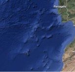
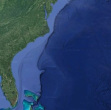
Figure 4.0.1: Satellite images. (a) North Atlantic Ocean, West coast; (b) North Atlantic Ocean, East coast; (c) Gulf of Trieste, Italy.

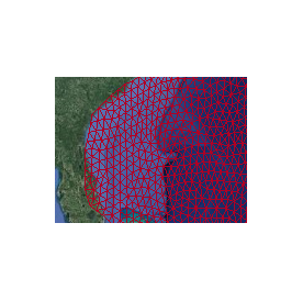
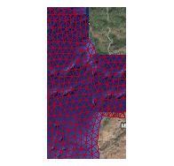
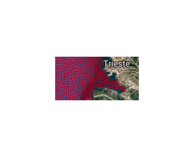
Figure 4.0.2: Meshes overlapping satellite images. (a) North Atlantic Ocean, particular of the Florida peninsula; (b) North Atlantic Ocean, particular of Portugal and North Africa; (c) Gulf of Trieste, particular of the city of Trieste.

The simulations have been run using FEniCS [34] for the full order solutions and RBniCS for the reduced order ones [26, 3]. The machine used for the simulations has a processor AMD A8-6410 APU with 8 GB of RAM.

4.1 Reduced Basis Applied to a Pollutant Control on the Gulf of Trieste

The proposed problem aims at limiting the impact of a pollutant tracer on touristic and natural areas of the Gulf of Trieste. The OCP($\boldsymbol{\mu}$) is governed by advection-diffusion state equation (see [18, 42, 43]). Let $\Omega$ be an open, bounded and regular domain representing the Gulf of Trieste (see Figure 4.1.1 (b)), with boundary $\partial\Omega=\Gamma_{D}\cup\Gamma_{N}$ and $\Gamma_{D}\cap\Gamma_{N}=\emptyset$, where homogeneous Dirichlet and Neumann boundary conditions are imposed on $\Gamma_{D}$ and $\Gamma_{N}$, respectively. The coasts are considered in $\Gamma_{D}$, while the open sea represents $\Gamma_{N}$ (see Figure 4.1.1 (c)).
Let us define the state and the control spaces as $Y=H^{1}_{\Gamma_{D}}(\Omega)=\displaystyle\{y\in H^{1}(\Omega)\;:\>y_{|\Gamma_{D}}=0\},$ and $U=\mathbb{R}$, respectively. We remark that the adjoint space is equal to the state space.
The non-dimensional OCP($\boldsymbol{\mu}$) reads: given $\boldsymbol{\mu}\in\mathcal{P}$, find $(y(\boldsymbol{\mu}),u(\boldsymbol{\mu}))\in Y\times U$ such that:

$$\begin{matrix}\underset{(y,u)\in Y\times U}{\text{min }}J(y,u)=\underset{(y,u)\in Y\times U}{\text{min }}\hskip 5.69046pt\displaystyle\frac{1}{2}\int_{\Omega_{OBS}}(y-y_{d})^{2}\;d\Omega_{OBS}\;\color[rgb]{0,0,0}{+\frac{\alpha}{2}\int_{\Omega_{u}}u^{2}\;d\Omega_{u}}\color[rgb]{0,0,0}\vspace{.5cm}\\ \text{such that }a(y,q;\boldsymbol{\mu})=c(u,q),\hskip 28.45274pt\forall q\in\color[rgb]{0,0,0}{Y}\color[rgb]{0,0,0}.\end{matrix}$$ (4.1.1)

where the state $y$ is the pollutant concentration and $y_{d}=0.2\in\mathbb{R}$ represents the safety threshold of the pollutant tracer.

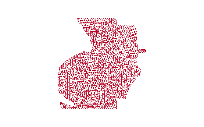
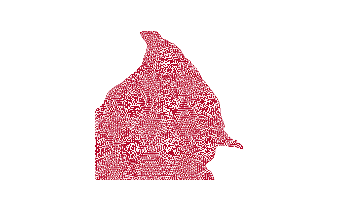
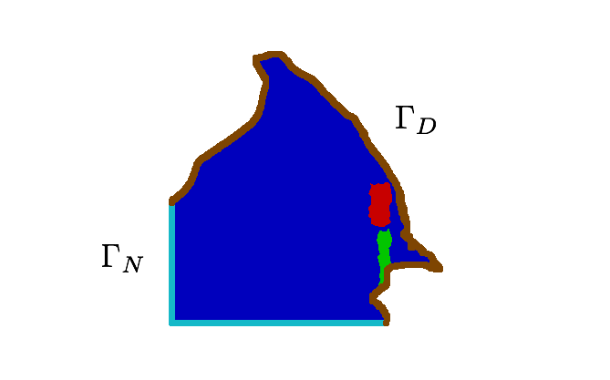
(a) Boundaries: light blue: open sea; brown: coasts. Subdomains: red: monitored natural area; green: source of the pollutant tracer.

Figure 4.1.1: Mesh and subdomains. (a) mesh of the North Atlantic Ocean; (b) mesh of the Gulf of Trieste; (c) subdomains of the Gulf of Trieste.

The bilinear forms $a:Y\times\color[rgb]{0,0,0}{Y}\color[rgb]{0,0,0}\rightarrow\mathbb{R}$ and $c:U\times\color[rgb]{0,0,0}{Y}\color[rgb]{0,0,0}\rightarrow\mathbb{R}$ are defined as:

$$\displaystyle a(y,q,\boldsymbol{\mu})=\int_{\Omega}(\nu(\boldsymbol{\mu})\nabla y\cdot\nabla q+\boldsymbol{\beta}(\boldsymbol{\mu})\cdot\nabla yq)\;d\Omega, \displaystyle c(u,q)=L\>u\int_{\Omega_{u}}q\>d\Omega_{u}.$$

where $\nu(\boldsymbol{\mu})\equiv\mu_{1}$ represents the diffusivity action of the state equation, while $\boldsymbol{\beta}(\boldsymbol{\mu})=[\beta_{1}(\mu_{2}),\beta_{2}(\mu_{3})]$ is the transport field acting on the Gulf. Then, the parameter $\boldsymbol{\mu}=[\mu_{1},\mu_{2},\mu_{3}]$ influences the circulation of the current in the Gulf. In this case $G\in\color[rgb]{0,0,0}{Y}{}^{\ast}$ is $G\equiv 0$. In this experiment, the control represents the concentration of the pollutant tracer released in the green area of the Gulf (see Figure 4.1.1 (c)) The constant $L=10^{3}$ makes the system non-dimensional. For the transport field we decided to take into consideration in proximity of the observation domain

$$\beta_{1}(\mu_{2})\equiv\mu_{2},\hskip 28.45274pt\beta_{2}(\mu_{3})\equiv\mu_{3}.$$

The parameter space considered is $\mathcal{P}=[0.5,1]\times[-1,1]\times[-1,1]$. The plot of the Figure 4.1.1 (c) shows the considered subdomains: in green $\Omega_{u}$, where the pollutant loss is, in red $\Omega_{OBS}$, where we want to monitor the pollutant concentration: it represents the swimming touristic area of the city and Miramare natural area (red subdomain in Figure 4.1.1). Two argumentations drove us in the choice of $\Omega_{OBS}$ (as underlined in [36]):

1. its unique ecological flora and fauna marine population,

2. it is an area crowded by Trieste citizens and by many tourists.

The parameter $\boldsymbol{\mu}$ is a physical parameter that describes the dynamic of the currents deriving from the specific winds blowing on this geographical area (the winds acting on the Gulf will be introduced later). Varying the parameter, it is possible to simulate several configurations in order to study how the wind could affect the diffusion of a dangerous pollutant in the natural area of Miramare. Thanks to reduced order modelling, many scenarios could be analysed, with a great saving of computational time resources. Several possible results must be taken into consideration in this context and, then, a deeper analysis can be made in order to better understand possible scenarios. The monitoring of the diffusion of a pollutant is necessary in order to preserve natural areas or to safeguard an ecological polluted habitat in case of ecological accident, and an accurate and fast model is helpful in planning a program of action.
In order to recast the problem in the framework (2.1.7), let $X=Y\times U$ be the product space of state and control spaces. Let $x=(y,u)$ and $w=(z,v)$ be elements of $X$, whereas $q$ an element of $\color[rgb]{0,0,0}{Y}\color[rgb]{0,0,0}$. Moreover, we define the bilinear forms $m:Y\times Y\rightarrow\mathbb{R}$ and $n:U\times U\rightarrow\mathbb{R}$ as follows:

$$\begin{matrix}m(y,z)=\displaystyle\int_{\Omega_{OBS}}yz\;d\Omega_{OBS}\;\;\;\text{ and }\vspace{.5cm}&\color[rgb]{0,0,0}{n(u,v)=\displaystyle\int_{\Omega_{u}}uv\;d\Omega_{u}}\color[rgb]{0,0,0}.\\ \end{matrix}$$

Furthermore, we define the forms $\mathcal{A},\mathcal{B}$ and $F$ as follows:

$$\mathcal{A}:X\times X\rightarrow\mathbb{R}\hskip 28.45274pt \mathcal{A}(x,w)=m(y,z)\color[rgb]{0,0,0}{\>+\>\alpha n(u,v)}\color[rgb]{0,0,0},$$

$$\mathcal{B}:X\times\color[rgb]{0,0,0}{Y}\color[rgb]{0,0,0}\rightarrow\mathbb{R}\hskip 28.45274pt \mathcal{B}(w,q;\boldsymbol{\mu})=a(z,q;\boldsymbol{\mu})-c(v,q),$$

$$F:X\rightarrow\mathbb{R}\hskip 28.45274pt \langle F,w\rangle=y_{d}\int_{\Omega_{OBS}}z\;d\Omega_{OBS}.$$

To build the aggregated reduced spaces for state and adjoint we used the POD-Galerkin algorithm introduced in section 3. In this specific example the reduced space for the control does not need to be reduced and thus we set $U_{N}=\mathbb{R}$. For this problem the affinity assumption is guaranteed: with $Q_{\mathcal{A}}=1$, $Q_{\mathcal{B}}=4$ and $Q_{F}=1$ the affine decomposition of the problem is given by

$$\Theta^{1}_{\mathcal{A}}=1\hskip 28.45274pt \mathcal{A}^{1}(x,w)=\mathcal{A}(x,w),$$

$$\Theta^{1}_{\mathcal{B}}=\mu_{1}\hskip 28.45274pt \mathcal{B}^{1}(x,q)=\int_{\Omega}\nabla y\cdot\nabla q\;d\Omega,$$

$$\Theta^{2}_{\mathcal{B}}=\mu_{2}\hskip 28.45274pt \mathcal{B}^{2}(x,q)=\int_{\Omega}\frac{\partial y}{\partial x_{1}}q\;d\Omega,$$

$$\Theta^{3}_{\mathcal{B}}=\mu_{3}\hskip 28.45274pt \mathcal{B}^{3}(x,q)=\int_{\Omega}\frac{\partial y}{\partial x_{2}}q\;d\Omega,$$

$$\Theta^{4}_{\mathcal{B}}=-L\hskip 28.45274pt \mathcal{B}^{4}(x,q)=\int_{\Omega_{u}}uq\;d\Omega,$$

$$\Theta^{1}_{F}=1\hskip 28.45274pt \langle F^{1},w\rangle=\langle F,w\rangle.$$

In the following, some numerical results linked to two different configurations are shown: the data of the experiments are reported in Table 4.1. As Figure 4.1.3 shows, the choice of a training set of $100$ snapshots was sufficient in order to achieve a good reduced approximation: the errors between FE and ROM variables have the same behaviour of the solution generated by a training set of $500$ truth approximations. We analysed how the wind action could influence pollutant diffusion. We simulated the net water transport due to Bora, a wind blowing from East to North-West, described by $(\mu_{2},\mu_{3})=(-1,1)$, and Scirocco, a wind blowing from South-East, corresponding to $(\mu_{2},\mu_{3})=(1,-1)$. From the lower value of the cost functional reported in Table 2, one can deduce that Bora makes the polluted water removed from $\Omega_{OBS}$, while Scirocco acts is the opposite way, pushing it towards the coast. Furthermore, Table 2 shows the differences between FE and ROM performances, in terms of dimension of the systems, time of resolution and cost functional. In Table 3 the speed up index behaviour with respect to the increasing of the basis numbers is presented. The speed up index represents the number of reduced problems solved in the time needed for a full order simulation. With the terminology basis number we refer to as the number $N$ such that $N_{y}=N_{p}=2N$ (and $N_{u}=1$, being $U=\mathbb{R}$), where $N_{y},N_{u},N_{p}$ are the number of online degrees of freedom for state, control and adjoint variable, respectively. In other words if the basis number is $N$, we are solving a system of dimension $(4N+1)\times(4N+1)$.
The first left plot in Figure 4.1.2 shows an “uncontrolled” Bora configuration (corresponding to $\boldsymbol{\mu}=(1,-1,1)$, resulting from the simulation of the state equation (only) with a value $u=1$ as a forcing term. Then, in the same Figure 4.1.2, the optimal control problem solution is presented with FE discretization and ROM, respectively. As one can see, the FE approximation and the ROM one match. Another proof of the reliability of reduced basis POD-Galerkin method is the pointwise error shown in the last plot of Figure 4.1.2: the maximum value reached is $1.373\cdot 10^{-10}$ with basis number $N=20$.

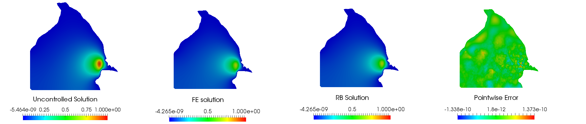
Figure 4.1.2: Gulf of Trieste (Bora configuration): results.

Table 1: Data of the numerical experiment: Gulf of Trieste.

Data	Bora Values	Scirocco Values
$\mu_{1}$	1	1
$(\mu_{2},\mu_{3})$	$(-1,1)$	$(1,-1)$
$y_{d}$	0.2	0.2
POD Training Set Dimension	100	100
Basis Number $N$	20	20
Sampling Distribution	uniform	uniform

Table 2: ROM vs FE: Gulf of Trieste (Bora configuration).

Bora Configuration	FE	ROM
System Dimension	$5939\times 5939$	$201\times 201$
Optimal Cost Functional	$4.9167\cdot 10^{-5}$	$4.9167\cdot 10^{-5}$
Time of Resolution	$2.79s$	$2.41\cdot 10^{-2}s$
Scirocco Configuration	FE	ROM
System Dimension	$5939\times 5939$	$201\times 201$
Optimal Cost Functional	$5.3417\cdot 10^{-5}$	$5.3417\cdot 10^{-5}$
Time of Resolution	$3.12s$	$3.41\cdot 10^{-2}s$

Table 3: Speed up analysis: Gulf of Trieste (Bora configuration).

Basis Number $N$	1	5	10	5	20
Speed up	361	364	350	317	296

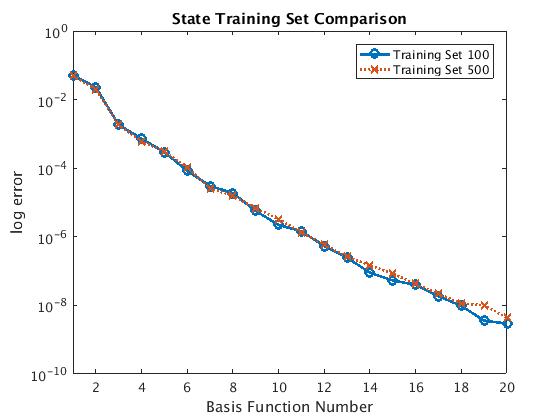
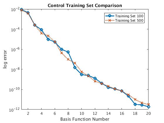
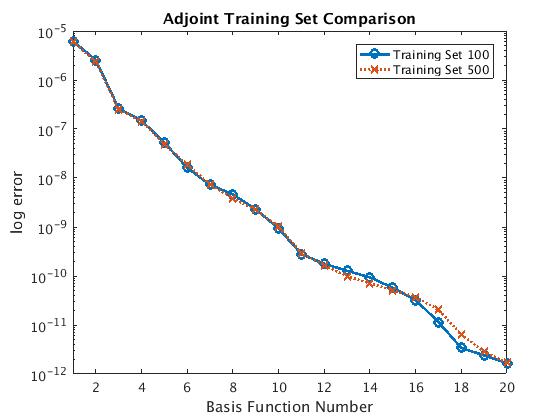
Figure 4.1.3: Gulf of Trieste (Bora configuration): errors and training set comparison. The plots are almost coincident.

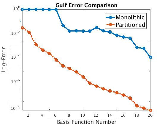
Figure 4.1.4: Gulf of Trieste (Bora configuration): errors.

In Figure 4.1.3 errors between FE solution and ROM solution with respect to the basis number $N$ over a random testing set of $100$ are presented. The obtained results show that the ROM allows to get fast and accurate simulations, since very few basis functions are required to have very small errors.
The plot in Figure 4.1.4 illustrates a comparison between the POD approach presented in section 3 (labeled as partitioned) and a different reduction in which only one POD is carried out for the variables $(y,u,p)$ at the same time on the space $X\times\color[rgb]{0,0,0}{Y}\color[rgb]{0,0,0}$ (labeled as monolithic). The results show that it is preferable to use a partitioned POD approach rather than a monolithic POD algorithm. The improvement is significant, since the latter approach gave an error of the order of $10^{-4}$ with $N=20$, while, for the same value of $N$ and with the partitioned option, the sum of the state, control and adjoint errors reaches the value of $10^{-8}$. Since the partitioned approach gave better values of the errors, we decided to exploit it for the Oceanographic application which we will present in the next section.

4.2 Reduced Basis Applied to an Ocean Circulation Solution Tracking

The general Ocean circulation model describes large scale flow dynamics. It is strictly linked to wind action: it can be considered as a coupled system of Ocean and Atmosphere. The theory associated to this topic is deeply analysed in [12, Chapter 3]. The model is governed by the following non-dimensional PDE($\boldsymbol{\mu}$), known as quasi-geostrophic equation:

$$\mu_{3}\mathcal{F}(\psi,\Delta\psi)+\frac{\partial\psi}{\partial x}=f-\mu_{1}\Delta\psi+\mu_{2}\Delta^{2}\psi,$$ (4.2.1)

where, given a suitable spaces $V$, the nonlinearity of the expression is given by $\mathcal{F}:V\times V\rightarrow\mathbb{R}$ defined as:

$$\mathcal{F}(\psi,q)=\frac{\partial\psi}{\partial x}\frac{\partial q}{\partial y}-\frac{\partial\psi}{\partial y}\frac{\partial q}{\partial x}.$$ (4.2.2)

The parameter $\mu_{3}$ represents how much the nonlinear term affects the flow dynamics, while $\mu_{1}$ and $\mu_{2}$ stand for diffusive action, respectively.
The parameter $\boldsymbol{\mu}$ describes the North Atlantic Ocean dynamics completely, since it gives information about how the large scale Ocean circulation is affected by different phenomena, such as location (typically described by $\mu_{3}$) and intensity variations of the gyres and the currents in the Ocean. Let us recall that Ocean dynamic is strongly linked to wind stress and atmospheric behaviour. Then, the parameter $\boldsymbol{\mu}$ describes the dynamic of a very complex physical system, taking into account several natural factors and phenomena. It is very important to run many simulations for different values of the parameter $\boldsymbol{\mu}$, in order to achieve a full knowledge of this system describing Oceanic and Atmospheric dynamics, linked to climatological forecasting issues.
As specified in [12, Section 3.2], the forcing term $f$ depends on wind stress $\boldsymbol{\tau}$ by the following relation:

$$f=\hat{\mathbf{k}}\cdot\text{rot }{\boldsymbol{\tau}},$$

where $\hat{\mathbf{k}}$ is the third reference spatial unit vector. In our application we considered a bounded and regular bi-dimensional domain $\Omega\subset\mathbb{R}^{2}$ representing the North Atlantic Ocean (see Figure 4.1.1 (a)). Furthermore, in this section, we focused on the linear version of the quasi-geostrophic equation ($\mu_{3}=0$). The nonlinear $OCP(\boldsymbol{\mu})$ governed the oceanographic model will be treated in section 5.2. The solution tracking problem constrained to this particular state equation is:

$$\underset{(\psi,u)\in V\times U}{\text{min }}J(\psi,u)=\underset{(\psi,u)\in V\times U}{\text{min }}\hskip 5.69046pt\frac{1}{2}\int_{\Omega}(\psi-\psi_{d})^{2}\;d\Omega+\frac{\alpha}{2}\int_{\Omega}u^{2}\;d\Omega\vspace{0.2cm}$$ (4.2.3)

$$\qquad\text{such that }\hskip 14.22636pt\begin{cases}\displaystyle\frac{\partial\psi}{\partial x}=u-\displaystyle\mu_{1}\Delta\psi+\mu_{2}\Delta^{2}\psi&\text{in }\Omega,\\ \psi=0&\text{on }\partial\Omega,\\ \Delta\psi=0&\text{on }\partial\Omega,\end{cases}$$

where $\psi\in V$ is our state variable, $u\in U$ is the forcing term to be controlled, where $V$ and $U$ are two suitable functions spaces and $\alpha$ is the penalization term. The physical parameter $\boldsymbol{\mu}=(\mu_{1},\mu_{2})$ is considered in the parametrized space $\mathcal{P}=[10^{-4},1]\times[10^{-4},1]$. In this example, the control variable represents the wind action. We stress that the quasi–geostrophic model describes how Ocean and Atmosphere interact. The problem aims at making the solution $\psi$ the most similar to $\psi_{d}$, representing the desired Ocean dynamics, thanks to the action of to the wind stress expressed by $u$, as mentioned above.
In some applications $\psi_{d}$ can represent experimental data. In this sense, our experiment could be seen as a prototype of a data assimilation model with forecasting purposes (see [5, 10, 11, 23, 29, 53] as references). This particular technique changes the model in order to achieve a solution comparable with real experimental data. Data assimilation techniques are very costly, and reduced order methods fit very well in this context. The proposed experiment helps to understand how reduced order techniques could be exploited in order to simulate several climatological scenarios in a low dimensional and accurate framework. The opportunity of running the reduced model many times allow us to have a deeper comprehension of the Ocean dynamic, and of atmospheric phenomena and climatological scenarios.
In order to manage a handier problem, we rewrite the previous system as it follows:

$$\underset{((\psi,q),u)\in Y\times U}{\text{min }}J((\psi,q),u)=\underset{((\psi,q),u)\in Y\times U}{\text{min }}\hskip 5.69046pt\frac{1}{2}\int_{\Omega}(\psi-\psi_{d})^{2}\;d\Omega+\frac{\alpha}{2}\int_{\Omega}u^{2}\;d\Omega\vspace{0.2cm}$$ (4.2.4)

$$\qquad\text{such that }\hskip 14.22636pt\begin{cases}q=\Delta\psi&\text{in }\Omega,\\ \displaystyle\frac{\partial\psi}{\partial x}=+u-\displaystyle\mu_{1}q+\mu_{2}\Delta q&\text{in }\Omega,\\ \psi=0&\text{on }\partial\Omega,\\ q=0&\text{on }\partial\Omega,\end{cases}$$

where the spaces are defined as $Y=H^{1}_{0}(\Omega)\times H^{1}_{0}(\Omega)$ and $U=L^{2}(\Omega)$. The weak formulation reads as:

$$a((\psi,q),(\phi,r);\boldsymbol{\mu})=c(u,(\phi,r))\hskip 28.45274pt\forall\phi,r\in H^{1}_{0}(\Omega),$$ (4.2.5)

where $a:Y\times Y\rightarrow\mathbb{R}$ and $c:U\times Y\rightarrow\mathbb{R}$ are given by:

$$\displaystyle a((\psi,q),(\phi,r);\boldsymbol{\mu}) =\int_{\Omega}\frac{\partial\psi}{\partial x}r\;d\Omega\displaystyle+\mu_{2}\int_{\Omega}\nabla q\cdot\nabla r\;d\Omega\;\displaystyle+\mu_{1}\int_{\Omega}qr\;d\Omega\displaystyle+\int_{\Omega}q\phi\;d\Omega\displaystyle+\int_{\Omega}\nabla\psi\cdot\nabla\phi\;d\Omega,\vspace{0.2cm}$$ (4.2.6)

$$\displaystyle c(u,(\phi,r)) =\int_{\Omega}ur\;d\Omega.$$ (4.2.7)

In this case $G\in\color[rgb]{0,0,0}{Y}{}^{\ast}$ is $G\equiv 0$.
Since we are facing a linear quadratic optimal control problem, it can be recast in saddle-point formulation (2.1.7). Let us define the product space $X=Y\times U$ and let $x=((\psi,q),u)$ and $w=((\chi,t),v)$ be two elements of $X$, whereas let $s=(\phi,r)$ be an element of the adjoint space. Furthermore, one has to specify:

$$\mathcal{A}:X\times X\rightarrow\mathbb{R}\hskip 28.45274pt \mathcal{A}(x,w)=m((\psi,q),(\chi,t))+\alpha n(u,v),$$

$$\mathcal{B}:X\times\color[rgb]{0,0,0}{Y}\color[rgb]{0,0,0}\rightarrow\mathbb{R}\hskip 28.45274pt \mathcal{B}(w,s;\boldsymbol{\mu})=a((\chi,t),(\phi,r),\boldsymbol{\mu})-c(v,(\phi,r)),$$

$$F:X\rightarrow\mathbb{R}\hskip 28.45274pt \langle F,w\rangle=\int_{\Omega}\psi_{d}\chi\;d\Omega,$$

where $m:Y\times Y\rightarrow\mathbb{R}$ and $n:U\times U\rightarrow\mathbb{R}$ are defined as

$$\begin{matrix}\displaystyle m((\psi,q),(\chi,t))=\int_{\Omega}\psi\chi\;d\Omega,&\displaystyle n(u,v)=\int_{\Omega}uv\;d\Omega.\\ \end{matrix}$$

In order to build the aggregated reduced spaces of the type proposed in section 3.3 a POD-Galerkin algorithm has been exploited. As we underlined in section 3.3, the affinity assumption must be guaranteed for the efficiency of the reduced problem. Indeed, with $Q_{\mathcal{A}}=1$, $Q_{\mathcal{B}}={\color[rgb]{0,0,0}3}$ and $Q_{F}=1$ the affine decomposition of the problem is given by

$$\Theta^{1}_{\mathcal{A}}=1\hskip 28.45274pt \mathcal{A}^{1}(x,w)=\mathcal{A}(x,w),$$

$$\Theta^{1}_{\mathcal{B}}=\mu_{1}\hskip 28.45274pt \mathcal{B}^{1}(x,s)=\int_{\Omega}qr\;d\Omega,$$

$$\Theta^{2}_{\mathcal{B}}=\mu_{2}\hskip 28.45274pt \mathcal{B}^{2}(x,s)=\int_{\Omega}\nabla q\cdot\nabla r\;d\Omega,$$

$$\Theta^{3}_{\mathcal{B}}=1\hskip 28.45274pt \mathcal{B}^{3}(x,s)=\int_{\Omega}\frac{\partial\psi}{\partial x}r\;d\Omega+\int_{\Omega}q\phi\;d\Omega+\int_{\Omega}\nabla\psi\cdot\nabla\phi\;d\Omega-\int_{\Omega}ur\;d\Omega,$$

$$\Theta^{1}_{F}=1\hskip 28.45274pt \langle F^{1},w\rangle=\langle F,w\rangle.$$

Table 4: Data of the numerical experiment: North Atlantic Ocean linear solution tracking.

Data	Values
$(\mu_{1},\mu_{2},\alpha)$	$(10^{-4},0.07^{3},10^{-5})$
	FE solution of
$\psi_{d}$	quasi-geostrophic equation
	with $f=-\sin(\pi y)$
	and $\boldsymbol{\mu}=(10^{-4},0.07^{3})$
POD Training Set Dimension	100
Basis Number $N$	25
Sampling Distribution	log-uniform

In Table 4 the data of the experiment are shown: choosing a training set of 100 generating elements gives comparable results with respect the one achieved with a training set generated by 500 snapshots, as presented in the errors plotted in Figure 4.2.2. In Figure 4.2.1 the desired $\psi_{d}$ value to be reached is presented with the FE and ROM solutions. The approximated solutions match. The last plot of the Figure 4.2.1 shows the pointwise error: the maximum value reached is $1.8\cdot 10^{-8}$ with basis number $N=25$.

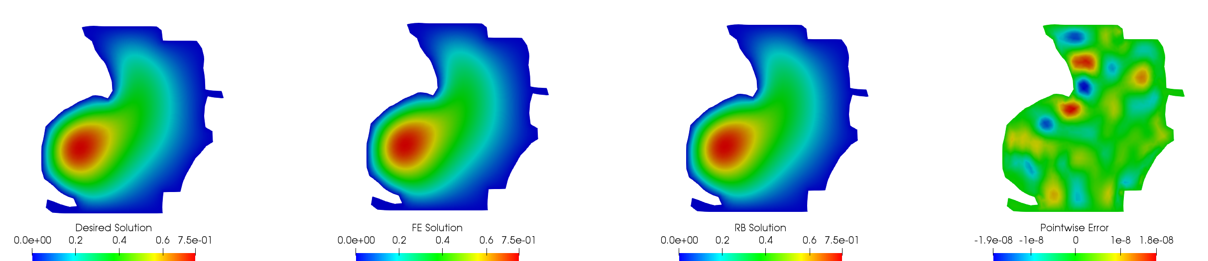
Figure 4.2.1: North Atlantic Ocean linear solution tracking: results.

The following tables represent the comparison between ROM and FE performances, in terms of: system dimension, cost functional optimal value, time of resolution (Table 5) and speed up index with respect to the basis number $N$ such that $2N=N_{\psi}=N_{q}=N_{\chi}=N_{t}$ and $N=N_{u}$ (Table 6), which results in a solution of a $9N\times 9N$ linear system. We can deduce how the ROM method is a suitable and convenient approach to study large scale phenomena in oceanography, a field dealing with parametrized simulations that require days of CPU times for complex configurations.

Table 5: ROM vs FE: North Atlantic Ocean linear solution tracking.

	FE	ROM
System Dimension	$6490\times 6490$	$450\times 450$
Optimal Cost Functional	$1.520\cdot 10^{-6}$	$1.520\cdot 10^{-6}$
Time of Resolution	$6.07s$	$2.03\cdot 10^{-1}s$

Table 6: Speed up analysis: North Atlantic Ocean linear solution tracking.

Basis Number ${\color[rgb]{0,0,0}N}$	1	5	10	15	20	25
Speed up	1049	395	192	207	199	33

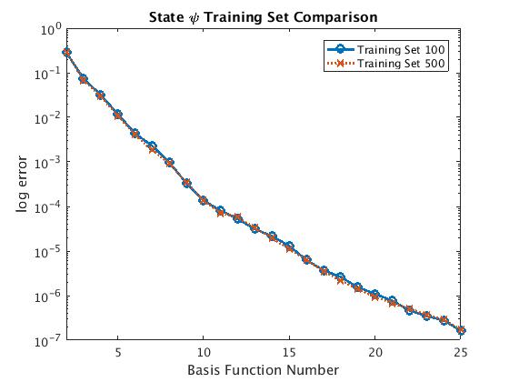
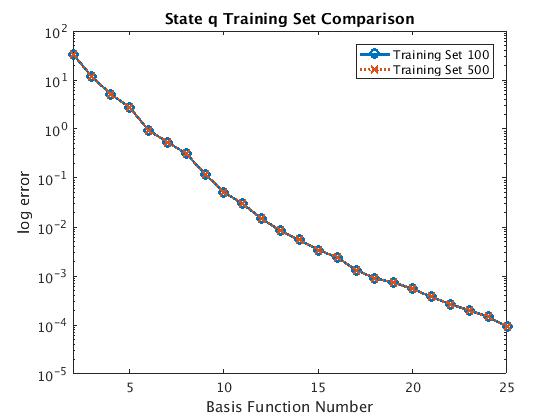
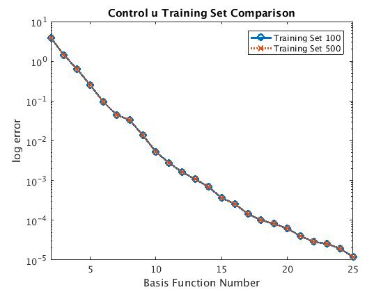
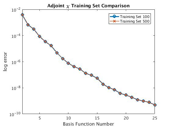
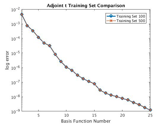
Figure 4.2.2: North Atlantic Ocean linear solution tracking: errors and training set comparison. The plots are coincident.

In Figure 4.2.2 the error norm between the FE approximation and the ROM discretization over a random testing set of $100$ is shown for all the variables, state $\psi$ and $q$, control $u$, and adjoint $\chi$ and $t$, respectively.

5 Nonlinear version of the Ocean Circulation Solution Tracking

This section aims at introducing a nonlinear version of the Oceanographic solution tracking proposed in section 4.2. First of all, the problem will be presented in a general theoretical formulation, then the $OCP(\boldsymbol{\mu})$ will be specified to the nonlinear quasi-geostrophic equations. As we did for the linear case, some numerical results will be presented, in order to sustain the idea of the great versatility of the ROMs in these kind of applications.

5.1 Nonlinear reduced OCP($\boldsymbol{\mu}$)s: a brief introduction

In the following section we want to briefly describe nonlinear OCP($\boldsymbol{\mu}$)s, in order to make the reader acquainted with the nonlinear numerical example presented. Let us introduce all the quantities needed, following the structure already exploited in section 2.1. We remark that, as in the linear case, in the different definitions, the dependence from the parameter $\boldsymbol{\mu}$ is sometimes understood.
Let $\Omega\subset\mathbb{R}^{n}$ be an open regular domain of boundary $\partial\Omega$. Let us introduce the Hilbert spaces $Y$, $U$ and $Z\supseteq Y$, where $Y$ is used both for the state and for the adjoint space, $U$ is the control space and $Z$ is the observation space. With a totally analogous procedure with respect the one exploited in (2.1.1), we can define the nonlinear constraint equation:

$$a_{\text{nl}}(y,q;\boldsymbol{\mu})=c(u,q;\boldsymbol{\mu})+\langle G(\boldsymbol{\mu}),q\rangle\hskip 28.45274pt\forall q\in Y,$$ (5.1.1)

where $a_{\text{nl}}:Y\times Y\rightarrow\mathbb{R}$ represents a continuous nonlinear state operator, $c:U\times Y\rightarrow\mathbb{R}$ is the usual continuous bilinear form linked to the control variable and $G\in Y^{\ast}$ gives us information about forcing and boundary terms. The subscript “nl” highlights the nonlinearity of the governing state equation. Set a constant $\alpha>0$, we can consider again the linear quadratic objective functional (2.1.2) where the roles of $y_{d}(\boldsymbol{\mu})\in Z$, $m:Z\times Z\rightarrow\mathbb{R}$ and $n:U\times U\rightarrow\mathbb{R}$ remain the same of the linear case in section 2.1. The OCP($\boldsymbol{\mu}$) reads as the problem (2.1.3), with the only difference that the constraint is nonlinear.
Let us define the product space $X=Y\times U$, endowed with the same scalar product and the same norm introduced in section 2.1. Taking $x=(y,u)$ and $w=(z,v)$ as two elements of $X$, we can define the following quantities:

$$\mathcal{A}:X\times X\rightarrow\mathbb{R} \mathcal{A}(x,w;\boldsymbol{\mu})=m(y,z;\boldsymbol{\mu})+\alpha n(u,v;\boldsymbol{\mu})\hskip 28.45274pt \forall x,w\in X,$$

$$\mathcal{B}_{\text{nl}}:X\times Y\rightarrow\mathbb{R} \mathcal{B}_{\text{nl}}(w,q;\boldsymbol{\mu})=a_{\text{nl}}(z,q;\boldsymbol{\mu})-c(v,q;\boldsymbol{\mu})\hskip 28.45274pt \forall w\in X,\;\forall q\in Y,$$

$$F(\boldsymbol{\mu})\in X^{\ast} \langle F(\boldsymbol{\mu}),w\rangle=m(y_{d}(\boldsymbol{\mu}),z;\boldsymbol{\mu})\hskip 28.45274pt \forall w\in X.$$

Thanks to these definitions and taking into consideration the adjoint variable $p\in Y$ , we can define, as in the linear case, the functional (2.1.4) and the new Lagrangian functional $\mathscr{L}^{\text{nl}}:Y\times U\times Y\rightarrow\mathbb{R}$ as

$$\mathscr{L}^{\text{nl}}(y,u,p;\boldsymbol{\mu})=\mathcal{J}((y,u);\boldsymbol{\mu})+\mathcal{B}_{\text{nl}}((y,u),p;\boldsymbol{\mu})-\langle G(\boldsymbol{\mu}),p\rangle.$$ (5.1.2)

In literature (see e.g. [27]) it is well known that solve the nonlinear minimisation problem (2.1.3) is equivalent to solving the following system: given $\boldsymbol{\mu}\in\mathcal{P}$, find $(x(\boldsymbol{\mu}),p(\boldsymbol{\mu}))\in X\times Y$, where $x(\boldsymbol{\mu})=(y(\boldsymbol{\mu}),u(\boldsymbol{\mu}))$, such that

$$\begin{cases}D_{y}\mathscr{L}^{\text{nl}}(y,u,p;\boldsymbol{\mu})[z]=0&\forall z\in Y,\\ D_{u}\mathscr{L}^{\text{nl}}(y,u,p;\boldsymbol{\mu})[v]=0&\forall v\in U,\\ D_{p}\mathscr{L}^{\text{nl}}(y,u,p;\boldsymbol{\mu})[q]=0&\forall q\in Y.\\ \end{cases}$$ (5.1.3)

$D_{y}\mathscr{L}^{\text{nl}}(y,u,p;\boldsymbol{\mu}),D_{u}\mathscr{L}^{\text{nl}}(y,u,p;\boldsymbol{\mu})$ and $D_{p}\mathscr{L}^{\text{nl}}(y,u,p;\boldsymbol{\mu})$ represent the differentiation of the Lagrangian functional (5.1.2) with respect to the state, the control ad the adjoint variable, respectively.
Following the analogous argument proposed in section 2.2, we consider $Y^{\mathcal{N}}$ and $U^{\mathcal{N}}$ as the Finite Element discretization for $Y$ and $U$, respectively. Also in this case, we define the discrete product space $X^{\mathcal{N}}=Y^{\mathcal{N}}\times U^{\mathcal{N}}\subset X$ and the Galerkin Finite Element discretized version of the problem (5.1.3) as: given $\boldsymbol{\mu}\in\mathcal{P}$, find $(x^{\mathcal{N}}(\boldsymbol{\mu}),p^{\mathcal{N}}(\boldsymbol{\mu}))\in X^{\mathcal{N}}\times Y^{\mathcal{N}}$, where $x^{\mathcal{N}}(\boldsymbol{\mu})=(y^{\mathcal{N}}(\boldsymbol{\mu}),u^{\mathcal{N}}(\boldsymbol{\mu}))$, such that

$$\begin{cases}D_{y^{\mathcal{N}}}\mathscr{L}^{\text{nl}}(y^{\mathcal{N}},u^{\mathcal{N}},p^{\mathcal{N}};\boldsymbol{\mu})[z^{\mathcal{N}}]=0&\forall z^{\mathcal{N}}\in Y^{\mathcal{N}},\\ D_{u^{\mathcal{N}}}\mathscr{L}^{\text{nl}}(y^{\mathcal{N}},u^{\mathcal{N}},p^{\mathcal{N}};\boldsymbol{\mu})[v^{\mathcal{N}}]=0&\forall v^{\mathcal{N}}\in U^{\mathcal{N}},\\ D_{p^{\mathcal{N}}}\mathscr{L}^{\text{nl}}(y^{\mathcal{N}},u^{\mathcal{N}},p^{\mathcal{N}};\boldsymbol{\mu})[{q^{\mathcal{N}}}]=0&\forall q^{\mathcal{N}}\in Y^{\mathcal{N}},\\ \end{cases}$$ (5.1.4)

where the discrete Lagrangian functional have been differentiated with respect to the discrete variables. Numerically, the discrete OCP($\boldsymbol{\mu}$) problem (5.1.4) has been solved through Newton’s methods. Since we are able to solve truth problems, we can consider the construction of reduced basis functions exploiting the POD-Galerkin procedure illustrated in section 3.2. Thanks to the POD-Galerkin algorithm we can reduce the Finite Element spaces $Y^{\mathcal{N}}$ and $U^{\mathcal{N}}$ and consider $Y_{N}$ and $U_{N}$, respectively. Then we can consider the space $X_{N}=Y_{N}\times U_{N}$ and the reduced nonlinear OCP($\boldsymbol{\mu}$) to be solved is defined as: given $\boldsymbol{\mu}\in\mathcal{P}$, find $(x_{N}(\boldsymbol{\mu}),p_{N}(\boldsymbol{\mu}))\in X_{N}\times Y_{N}$, where $x_{N}(\boldsymbol{\mu})=(y_{N}(\boldsymbol{\mu}),u_{N}(\boldsymbol{\mu}))$, such that

$$\begin{cases}D_{y_{N}}\mathscr{L}^{\text{nl}}(y_{N},u_{N},p_{N};\boldsymbol{\mu})[z_{N}]=0&\forall z_{N}\in Y_{N},\\ D_{u_{N}}\mathscr{L}^{\text{nl}}(y_{N},u_{N},p_{N};\boldsymbol{\mu})[v_{N}]=0&\forall v_{N}\in U_{N},\\ D_{p_{N}}\mathscr{L}^{\text{nl}}(y_{N},u_{N},p_{N};\boldsymbol{\mu})[q_{N}]=0&\forall q_{N}\in Y_{N},\\ \end{cases}$$ (5.1.5)

We recall that the affinity assumption must be verified in order to guarantee good performances of the ROM methods. Since the case of interest contains only quadratically nonlinear terms, the affinity assumption can be guaranteed by storing the appropriate nonlinear terms in third order tensors. In more general cases one can resort e.g. to empirical interpolation [4] and later variants. We exploited the Newton’s method to solve the reduced problem (5.1.5), as we did for the did for the discretized version (5.1.4).

5.2 Reduced Basis Applied to a Nonlinear Ocean Circulation Solution Tracking

We recall that the general Ocean circulation model governing large scale flow dynamics presented in [12, Chapter 3] is described by the nonlinear equation (4.2.1). The nonlinearity of the model is given by the expression (4.2.2). In this experiment, the physical parameter $\boldsymbol{\mu}=(\mu_{1},\mu_{2},\mu_{3})$ takes values in the parameter space $\mathcal{P}=[0.07^{3},1]\times[10^{-4},1]\times[10^{-4},0.045^{2}]$. As in section 4.2, $\mu_{1}$ and $\mu_{2}$ represent the diffusive action of the Ocean, while $\mu_{3}$ is the parameter linked to its nonlinear dynamic. The range for the parameters ensures stability to the problem and allow us to treat a moderate nonlinear OCP($\boldsymbol{\mu}$) governed by quasi-geostrophic equations: in this work we will only deal with this specific case and we will not treat highly nonlinear problems, corresponding to lower values of $\mu_{1},\mu_{2}$ and/or higher values of $\mu_{3}$. We underline that the steady quasi-geostrophic model is a very complex physical system: in order to have a complete description of the meaning of the model and of the role of all its components the reader is referred to section 4.2 and to [12, Chapter 3]. The solution tracking problem constrained to the nonlinear quasi-geostrophic equation is:

$$\underset{(\psi,u)\in V\times U}{\text{min }}J(\psi,u)=\underset{(\psi,u)\in V\times U}{\text{min }}\hskip 5.69046pt\frac{1}{2}\int_{\Omega}(\psi-\psi_{d})^{2}\;d\Omega+\frac{\alpha}{2}\int_{\Omega}u^{2}\;d\Omega\vspace{0.2cm}$$ (5.2.1)

$$\qquad\text{such that }\hskip 14.22636pt\begin{cases}\displaystyle\frac{\partial\psi}{\partial x}=u-\displaystyle\mu_{1}\Delta\psi+\mu_{2}\Delta^{2}\psi-\mu_{3}\mathcal{F}(\psi,\Delta\psi)&\text{in }\Omega,\\ \psi=0&\text{on }\partial\Omega,\\ \Delta\psi=0&\text{on }\partial\Omega,\end{cases}$$

where $V$ and $U$ are suitable functional spaces, $\psi\in V$ is the state variable, $u\in U$ is the unknown wind action to be controlled and $\alpha$ is a penalization term. The aim of the OCP($\boldsymbol{\mu}$) presented is the same of its linear version (4.2.3): make our state solution the most similar to an already known desired state profile. As in the linear case, we rewrite problem (5.2.1) as:

$$\underset{((\psi,q),u)\in Y\times U}{\text{min }}J((\psi,q),u)=\underset{((\psi,q),u)\in Y\times U}{\text{min }}\hskip 5.69046pt\frac{1}{2}\int_{\Omega}(\psi-\psi_{d})^{2}\;d\Omega+\frac{\alpha}{2}\int_{\Omega}u^{2}\;d\Omega\vspace{0.2cm}$$ (5.2.2)

$$\qquad\text{such that }\hskip 14.22636pt\begin{cases}q=\Delta\psi&\text{in }\Omega,\\ \displaystyle\frac{\partial\psi}{\partial x}=u-\displaystyle\mu_{1}q+\mu_{2}\Delta q-\mu_{3}\mathcal{F}(\psi,q)&\text{in }\Omega,\\ \psi=0&\text{on }\partial\Omega,\\ q=0&\text{on }\partial\Omega,\end{cases}$$

where the spaces are defined as $Y=H^{1}_{0}(\Omega)\times H^{1}_{0}(\Omega)$ and $U=L^{2}(\Omega)$. The weak formulation of the nonlinear state equation is represented as:

$$a_{\text{nl}}((\psi,q),(\phi,r);\boldsymbol{\mu})=c(u,(\phi,r))\hskip 28.45274pt\forall\phi,r\in H^{1}_{0}(\Omega),$$ (5.2.3)

where $c:U\times Y\rightarrow\mathbb{R}$ is (4.2.7) and $a_{\text{nl}}:Y\times Y\rightarrow\mathbb{R}$ is given by:

$$a_{\text{nl}}((\psi,q),(\phi,r);\boldsymbol{\mu})=a((\psi,q),(\phi,r);\boldsymbol{\mu})-\mu_{3}\int_{\Omega}\psi\Big{(}\frac{\partial q}{\partial y}\frac{\partial r}{\partial x}-\frac{\partial q}{\partial x}\frac{\partial r}{\partial y}\Big{)}\;d\Omega,$$ (5.2.4)

where $a((\psi,q),(\phi,r);\boldsymbol{\mu})$ is defined in (4.2.6), and $G\in Y^{\ast}$ is $G\equiv 0$.
In the following, we aim at recasting the problem (5.2.2) in the framework proposed in (5.1.3). Let us define the product space $X=Y\times U$ and let $x=((\psi,q),u)$ and $w=((\chi,t),v)$ be two elements of $X$. Let us consider $s=(\phi,r)\in Y$ as our adjoint variable . Let us describe the following quantities:

$$\mathcal{A}:X\times X\rightarrow\mathbb{R}\hskip 28.45274pt \mathcal{A}(x,w)=m((\psi,q),(\chi,t))+\alpha n(u,v),$$

$$\mathcal{B}_{\text{nl}}:X\times Y\rightarrow\mathbb{R}\hskip 28.45274pt \mathcal{B}_{\text{nl}}(w,s;\boldsymbol{\mu})=a_{\text{nl}}((\chi,t),(\phi,r),\boldsymbol{\mu})-c(v,(\phi,r)),$$

$$F:X\rightarrow\mathbb{R}\hskip 28.45274pt \langle F,w\rangle=\int_{\Omega}\psi_{d}\chi\;d\Omega.$$

As in the linear version, the bilinear forms $m:Y\times Y\rightarrow\mathbb{R}$ and $n:U\times U\rightarrow\mathbb{R}$ are

$$m((\psi,q),(\chi,t))=\int_{\Omega}\psi\chi\;d\Omega\;\;\;\;\;\text{and}\;\;\;\;\displaystyle n(u,v)=\int_{\Omega}uv\;d\Omega.$$

In order to solve the OCP($\boldsymbol{\mu}$) governed by (5.2.2), we define the Lagrangian functional (5.1.2) and we recall that $x=((\psi,q),u),w=((\chi,t),v)$. We also define a test function in the adjoint space $Y$ as $\eta=(\xi,\sigma)$. Then we solve the system (5.1.3) where:

$$D_{(\psi,q)}\mathscr{L}^{\text{nl}}((\psi,q),u,(\phi,r);\boldsymbol{\mu})[(\chi,t)]=m((\psi,q),(\chi,t))-\int_{\Omega}\frac{\partial r}{\partial x}\chi\ \;d\Omega\displaystyle+\mu_{2}\int_{\Omega}\nabla t\cdot\nabla r\;d\Omega\;+$$

$$\hskip 85.35826pt\qquad\qquad\displaystyle+\mu_{1}\int_{\Omega}tr\;d\Omega\displaystyle+\int_{\Omega}t\phi\;d\Omega\displaystyle+\int_{\Omega}\nabla\chi\cdot\nabla\phi\;d\Omega\;+\vspace{0.2cm}$$

$$\hskip 85.35826pt\ \qquad\qquad\qquad\qquad\displaystyle-\mu_{3}\int_{\Omega}\chi\Big{(}\frac{\partial q}{\partial y}\frac{\partial r}{\partial x}-\frac{\partial q}{\partial x}\frac{\partial r}{\partial y}\Big{)}\;d\Omega\;+$$ (5.2.5)

$$\hskip 85.35826pt\ \qquad\qquad\qquad\qquad\qquad\qquad\displaystyle-\mu_{3}\int_{\Omega}t\Big{(}\frac{\partial\psi}{\partial y}\frac{\partial r}{\partial y}-\frac{\partial r}{\partial x}\frac{\partial\psi}{\partial y}\Big{)}\;d\Omega-\int_{\Omega}u\chi-\langle F,w\rangle,$$

$$D_{u}\mathscr{L}^{\text{nl}}((\psi,q),u,(\phi,r);\boldsymbol{\mu})[v]=\alpha n(u,v)-\int_{\Omega}vr\;d\Omega,$$

$$D_{(\phi,r)}\mathscr{L}^{\text{nl}}((\psi,q),u,(\phi,r);\boldsymbol{\mu})[(\xi,\sigma)]=\mathcal{B}(x,\eta;\boldsymbol{\mu}).$$

We built the aggregated reduced spaces exploiting the partitioned POD-Galerkin algorithm for the five variables $\psi,q,u,\chi,t$ as proposed in section 3.2, separately. As we did for the other numerical simulations, we underline that the affinity assumption is guaranteed. Indeed, with $Q_{\mathcal{A}}=1$, $Q_{\mathcal{B}_{\text{nl}}}=4$ and $Q_{F}=1$ the affine decomposition of the problem is given by

$$\Theta^{1}_{\mathcal{A}}=1\hskip 28.45274pt \mathcal{A}^{1}(x,w)=\mathcal{A}(x,w),$$

$$\Theta^{1}_{\mathcal{B}_{\text{nl}}}=\mu_{1}\hskip 28.45274pt \mathcal{B}^{1}_{\text{nl}}(x,s)=\int_{\Omega}qr\;d\Omega,$$

$$\Theta^{2}_{\mathcal{B}_{\text{nl}}}=\mu_{2}\hskip 28.45274pt \mathcal{B}^{2}_{\text{nl}}(x,s)=\int_{\Omega}\nabla q\cdot\nabla r\;d\Omega,$$

$$\Theta^{3}_{\mathcal{B}_{\text{nl}}}=1\hskip 28.45274pt \mathcal{B}^{3}_{\text{nl}}(x,s)=\int_{\Omega}\frac{\partial\psi}{\partial x}r\;d\Omega+\int_{\Omega}q\phi\;d\Omega+\int_{\Omega}\nabla\psi\cdot\nabla\phi\;d\Omega-\int_{\Omega}ur\;d\Omega,$$

$$\Theta^{4}_{\mathcal{B}_{\text{nl}}}=-\mu_{3}\hskip 28.45274pt \mathcal{B}^{4}_{\text{nl}}(x,s)=\int_{\Omega}\psi\Big{(}\frac{\partial q}{\partial y}\frac{\partial r}{\partial x}-\frac{\partial q}{\partial x}\frac{\partial r}{\partial y}\Big{)}\;d\Omega,$$

$$\Theta^{1}_{F}=1\hskip 28.45274pt \langle F^{1},w\rangle=\langle F,w\rangle.$$

Table 7: Data of the numerical experiment: North Atlantic Ocean nonlinear solution tracking.

Data	Values
$(\mu_{1},\mu_{2},\mu_{3},\alpha)$	$(10^{-4},0.07^{3},0.045^{2},10^{-5})$
	FE solution of
$\psi_{d}$	nonlinear quasi-geostrophic equation
	with $f=-\sin(\pi y)$
	and $\boldsymbol{\mu}=(10^{-4},0.07^{3},0.07^{2},10^{-5})$
POD Training Set Dimension	100
Basis Number $N$	25
Sampling Distribution	log-equispaced

Table 7 shows all the features of this experiment. In Figure 5.2.1 the desired solution profile $\psi_{d}$ is presented. Then the truth and the reduced solutions are plotted. It can be seen that the approximated solutions match. In the last plot of Figure 5.2.1, the pointwise error is shown: the maximum value reached is $9.6\cdot 10^{-7}$ with basis number $N=25$. We recall that $2N=N_{\psi}=N_{q}=N_{\chi}=N_{t}$ and $N=N_{u}$. We also analysed the ROM and the FE performances, in terms of: system dimension, cost functional optimal value, time of resolution (Table 8). Table 9 presents the speed up index with respect to the basis number $N$. The results presented remark how the ROM approach could be a very suitable tool in order to solve quasi-geostrophic equations, most of all in their nonlinear version that describes more complicated, but more realistic, Ocean dynamics, like the movement of the flow stream towards North (Gulf Stream circulation). Figure 5.2.2 shows the error norm between FE and reduced variables as already indicated in footnote 7 over a random testing set of $50$, obtaining a similar behavior with respect to the linear case.

Table 8: ROM vs FE: North Atlantic Ocean nonlinear solution tracking.

	FE	ROM
System Dimension	$6490\times 6490$	$450\times 450$
Optimal Cost Functional	$2.04347\cdot 10^{6}$	$2.04346\cdot 10^{6}$
Time of Resolution	$7.21s$	$5.11\cdot 10^{-1}s$

Figure 5.2.1: North Atlantic Ocean nonlinear solution tracking: results.

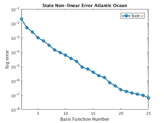
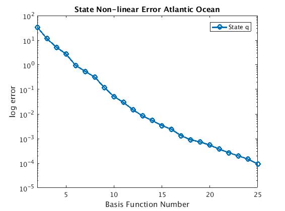
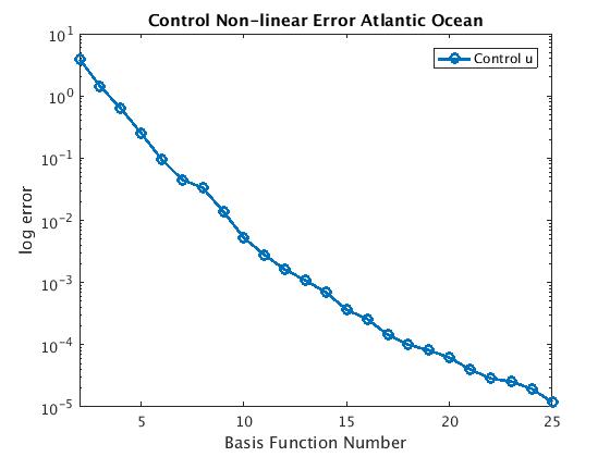
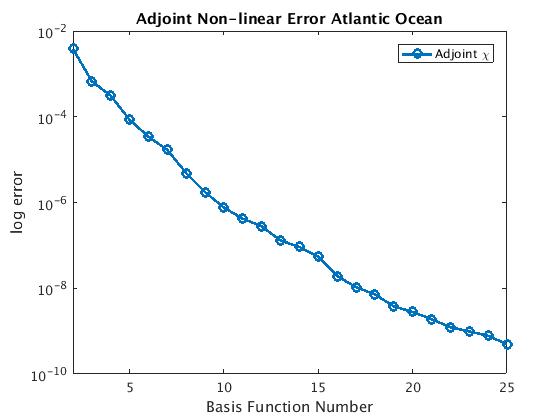
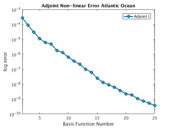
Figure 5.2.2: North Atlantic Ocean nonlinear solution tracking: errors.

Table 9: Speed up analysis: North Atlantic Ocean nonlinear solution tracking.

Basis Number ${\color[rgb]{0,0,0}N}$	1	5	10	15	20	25
Speed up	10	8	7	6	5	5

6 Conclusions and Perspectives

In this work we have exploited reduced order methods in environmental parametrized optimal control problems dealing with marine sciences and engineering. We proposed two specific examples: one representing the ecological issue of pollutant control in a specific naturalist area, the Gulf of Trieste, Italy, the other one consisting in a large scale solution tracking OCP($\boldsymbol{\mu}$) governed by quasi-geostrophic equations. We showed how reduced order methods could be a very useful tool in environmental sciences, like oceanography and ecology, where parametrized simulations are usually very demanding and costly. Reduced order methods are a suitable approach to face these issues. We have used a POD-Galerkin method for sampling and for the projection, by exploiting an aggregated space strategy. Reduced order methods performances have been compared to FE approximation, classically used to study these phenomena, in order to prove how convenient the reduced order approach could be in this particular field of applications: in the linear version of the North Atlantic problem, the reduced time of resolution decreases of one order of magnitude with respect to the full order one, and the error of the state variable $\psi$ is negligible. To the best of our knowledge, the main novelty of this work is in the POD-Galerkin reduction of a solution tracking optimal control problem governed by quasi-geostrophic equations in its linear and nonlinear version.
Let us expose some improvements of this work, focusing on the optimal control problem governed by quasi-geostrophic equation. A possible development would involve a time dependent optimal control problem considering also the highly nonlinear case. This kind of formulation is of the utmost importance in climatological applications, in order to forecast and predict possible scenarios in a reliable way. This complete model will make the problems more and more realistic and suited to actual ecological and climatological challenges, as well as more and more computational demanding. In this sense, reduced order modelling appears, again, to be a suitable and versatile approach to be used. Time dependent nonlinear optimal control problems insert themselves in the framework of data assimilation techniques, that, as briefly introduced in section 4.2, allow to modify the model in order to reach more reliable results in the forecasting applications, thanks to a solution tracking where the solution desired to be reached represents real experimental data.
For all the examples presented, a further step could be the development of three-dimensional marine model that could take into consideration bathimetry effect. Finally, the problems could be inserted in a reduced order uncertainty quantification context (see e.g. [52]), when it is not possible to assign specific values for the parameters by classical statistical methods.

References

- [1] Eduard Bader, Mark Kärcher, Martin A Grepl, and Karen Veroy. Certified reduced basis methods for parametrized distributed elliptic optimal control problems with control constraints. SIAM Journal on Scientific Computing, 38(6):A3921–A3946, 2016.
- [2] F. Ballarin, A. Manzoni, A. Quarteroni, and G. Rozza. Supremizer stabilization of POD–Galerkin approximation of parametrized steady incompressible Navier–Stokes equations. International Journal for Numerical Methods in Engineering, 102(5):1136–1161, 2015.
- [3] F. Ballarin, A. Sartori, and G. Rozza. RBniCS - reduced order modelling in FEniCS. http://mathlab.sissa.it/rbnics, 2015.
- [4] M. Barrault, Y. Maday, N. C. Nguyen, and A. T. Patera. An Empirical Interpolation Method: application to efficient reduced-basis discretization of partial differential equations. Comptes Rendus Mathematique, 339(9):667–672, 2004.
- [5] D. W Behringer, M. Ji, and A. Leetmaa. An improved coupled model for ENSO prediction and implications for Ocean initialization. Part I: The Ocean data assimilation system. Monthly Weather Review, 126(4):1013–1021, 1998.
- [6] P. B. Bochev and M. D. Gunzburger. Least-squares finite element methods, volume 166. Springer-Verlag, New York, 2009.
- [7] D. Boffi, F. Brezzi, and M. Fortin. Mixed finite element methods and applications, volume 44. Springer-Verlag, Berlin and Heidelberg, 2013.
- [8] F. Brezzi. On the existence, uniqueness and approximation of saddle-point problems arising from Lagrangian multipliers. Revue française d’automatique, informatique, recherche opérationnelle. Analyse numérique, 8(2):129–151, 1974.
- [9] John Burkardt, Max Gunzburger, and Hyung-Chun Lee. POD and CVT-based reduced-order modeling of navier–stokes flows. Computer Methods in Applied Mechanics and Engineering, 196(1-3):337–355, 2006.
- [10] J. A. Carton, G. Chepurin, X. Cao, and B. Giese. A simple Ocean data assimilation analysis of the global upper Ocean 1950–95. Part I: Methodology. Journal of Physical Oceanography, 30(2):294–309, 2000.
- [11] J. A. Carton and B. S. Giese. A reanalysis of ocean climate using Simple Ocean Data Assimilation (SODA). Monthly Weather Review, 136(8):2999–3017, 2008.
- [12] F. Cavallini and F. Crisciani. Quasi-geostrophic theory of Oceans and atmosphere: topics in the dynamics and thermodynamics of the Fluid Earth, volume 45. Springer Science & Business Media, New York, 2013.
- [13] D. Chapelle, A. Gariah, P. Moireau, and J. Sainte-Marie. A galerkin strategy with proper orthogonal decomposition for parameter-dependent problems: Analysis, assessments and applications to parameter estimation. ESAIM: Mathematical Modelling and Numerical Analysis, 47(6):1821–1843, 2013.
- [14] Peng Chen, Alfio Quarteroni, and Gianluigi Rozza. Multilevel and weighted reduced basis method for stochastic optimal control problems constrained by Stokes equations. Numerische Mathematik, 133(1):67–102, 2015.
- [15] J. C. de los Reyes and F. Tröltzsch. Optimal control of the stationary Navier-Stokes equations with mixed control-state constraints. SIAM Journal on Control and Optimization, 46(2):604–629, 2007.
- [16] L. Dedè. Optimal flow control for Navier-Stokes equations: Drag minimization. International Journal for Numerical Methods in Fluids, 55(4):347–366, 2007.
- [17] L. Dedè. Reduced basis method and a posteriori error estimation for parametrized linear-quadratic optimal control problems. SIAM Journal on Scientific Computing, 32(2):997–1019, 2010.
- [18] L. Dedè. Adaptive and reduced basis method for optimal control problems in environmental applications. PhD thesis, Politecnico di Milano, 2008. Available at http://mox.polimi.it.
- [19] Luca Dedè. Reduced basis method and error estimation for parametrized optimal control problems with control constraints. Journal of Scientific Computing, 50(2):287–305, Feb 2012.
- [20] M. C. Delfour and J. Zolésio. Shapes and geometries: metrics, analysis, differential calculus, and optimization, volume 22. SIAM, Philadelphia, 2011.
- [21] E. Fernández Cara and E. Zuazua Iriondo. Control theory: History, mathematical achievements and perspectives. Boletín de la Sociedad Española de Matemática Aplicada, 26, 79-140., 2003.
- [22] A. L. Gerner and K. Veroy. Certified reduced basis methods for parametrized saddle point problems. SIAM Journal on Scientific Computing, 34(5):A2812–A2836, 2012.
- [23] M. Ghil and P. Malanotte-Rizzoli. Data assimilation in meteorology and oceanography. Advances in geophysics, 33:141–266, 1991.
- [24] M. D. Gunzburger. Perspectives in flow control and optimization, volume 5. SIAM, Philadelphia, 2003.
- [25] J. Haslinger and R. A. E. Mäkinen. Introduction to shape optimization: theory, approximation, and computation. SIAM, Philadelphia, 2003.
- [26] J. S. Hesthaven, G. Rozza, and B. Stamm. Certified reduced basis methods for parametrized partial differential equations. SpringerBriefs in Mathematics, 2015, Springer, Milano.
- [27] M.L. Hinze, R. Pinnau, M. Ulbrich, and S. Ulbrich. Optimization with PDE constraints, volume 23. Springer Science & Business Media, Antwerp, 2008.
- [28] K. Ito and SS. Ravindran. A reduced-order method for simulation and control of fluid flows. Journal of computational physics, 143(2):403–425, 1998.
- [29] E. Kalnay. Atmospheric modeling, data assimilation and predictability. Cambridge university press, 2003, Cambridge.
- [30] Mark Kärcher and Martin A Grepl. A certified reduced basis method for parametrized elliptic optimal control problems. ESAIM: Control, Optimisation and Calculus of Variations, 20(2):416–441, 2014.
- [31] T.Y. Kim, T. Iliescu, and E. Fried. B-spline based finite-element method for the stationary quasi-geostrophic equations of the Ocean. Computer Methods in Applied Mechanics and Engineering, 286:168–191, 2015.
- [32] Karl Kunisch and Stefan Volkwein. Control of the burgers equation by a reduced-order approach using proper orthogonal decomposition. Journal of optimization theory and applications, 102(2):345–371, 1999.
- [33] Karl Kunisch and Stefan Volkwein. Proper orthogonal decomposition for optimality systems. ESAIM: Mathematical Modelling and Numerical Analysis, 42(1):1–23, 2008.
- [34] A. Logg, K.A. Mardal, and G. Wells. Automated Solution of Differential Equations by the Finite Element Method. Springer-Verlag, Berlin, 2012.
- [35] B. Mohammadi and O. Pironneau. Applied shape optimization for fluids. Oxford University Press, New York, 2010.
- [36] R. Mosetti, C. Fanara, M. Spoto, and E. Vinzi. Innovative strategies for marine protected areas monitoring: the experience of the Istituto Nazionale di Oceanografia e di Geofisica Sperimentale in the Natural Marine Reserve of Miramare, Trieste-Italy. In OCEANS, 2005. Proceedings of MTS/IEEE, pages 92–97. IEEE, 2005.
- [37] F. Negri. Reduced basis method for parametrized optimal control problems governed by PDEs. Master thesis, Politecnico di Milano, 2011.
- [38] F. Negri, A. Manzoni, and G. Rozza. Reduced basis approximation of parametrized optimal flow control problems for the Stokes equations. Computers & Mathematics with Applications, 69(4):319–336, 2015.
- [39] F. Negri, G. Rozza, A. Manzoni, and A. Quarteroni. Reduced basis method for parametrized elliptic optimal control problems. SIAM Journal on Scientific Computing, 35(5):A2316–A2340, 2013.
- [40] M. Pošta and T. Roubíček. Optimal control of Navier–Stokes equations by Oseen approximation. Computers & Mathematics With Applications, 53(3):569–581, 2007.
- [41] C. Prud’Homme, D. V. Rovas, K. Veroy, L. Machiels, Y. Maday, A. Patera, and G. Turinici. Reliable real-time solution of parametrized partial differential equations: Reduced-basis output bound methods. Journal of Fluids Engineering, 124(1):70–80, 2002.
- [42] A. Quarteroni, G. Rozza, L. Dedè, and A. Quaini. Numerical approximation of a control problem for advection-diffusion processes. In IFIP Conference on System Modeling and Optimization, pages 261–273, Ceragioli F., Dontchev A., Futura H., Marti K., Pandolfi L. (eds) System Modeling and Optimization. CSMO 2005. vol 199. Springer, Boston, 2005.
- [43] A. Quarteroni, G. Rozza, and A. Quaini. Reduced basis methods for optimal control of advection-diffusion problems. In Advances in Numerical Mathematics, pages 193–216. RAS and University of Houston, Moscow, 2007.
- [44] G. Rozza, D.B.P. Huynh, and A. Manzoni. Reduced basis approximation and a posteriori error estimation for Stokes flows in parametrized geometries: Roles of the inf-sup stability constants. Numerische Mathematik, 125(1):115–152, 2013.
- [45] G. Rozza, D.B.P. Huynh, and A.T. Patera. Reduced basis approximation and a posteriori error estimation for affinely parametrized elliptic coercive partial differential equations: Application to transport and continuum mechanics. Archives of Computational Methods in Engineering, 15(3):229–275, 2008.
- [46] G. Rozza, A. Manzoni, and F. Negri. Reduction strategies for PDE-constrained oprimization problems in Haemodynamics. pages 1749–1768, ECCOMAS, Congress Proceedings, Vienna, Austria, September 2012.
- [47] O. San and T. Iliescu. A stabilized proper orthogonal decomposition reduced-order model for large scale quasigeostrophic Ocean circulation. Advances in Computational Mathematics, 41(5):1289–1319, 2015.
- [48] J. Schöberl and W. Zulehner. Symmetric indefinite preconditioners for saddle point problems with applications to PDE-constrained optimisation problems. SIAM Journal on Matrix Analysis and Applications, 29(3):752–773, 2007.
- [49] V. Schulz and I. Gherman. One-shot methods for aerodynamic shape optimization. In MEGADESIGN and MegaOpt-German Initiatives for Aerodynamic Simulation and Optimization in Aircraft Design, pages 207–220. Springer, 2009.
- [50] T. Shiganova and A. Malej. Native and non-native ctenophores in the Gulf of Trieste, Northern Adriatic Sea. Journal of Plankton Research, 31(1):61–71, 2009.
- [51] S. Taasan. One shot methods for optimal control of distributed parameter systems 1: Finite dimensional control. Tech. report 91-2, Institute for Computer Applications in Science and Engineering, Hampton, VA, 1991.
- [52] D. Torlo, F. Ballarin, and G. Rozza. Weighted stabilized reduced basis methods for parametrized advection dominated problems with random inputs. Submitted, 2017.
- [53] E. Tziperman and W. C. Thacker. An optimal-control/adjoint-equations approach to studying the Oceanic general circulation. Journal of Physical Oceanography, 19(10):1471–1485, 1989.
- [54] H. Yang, G. Lohmann, W. Wei, M.I. Dima, M. Ionita, and J. Liu. Intensification and poleward shift of subtropical western boundary currents in a warming climate. Journal of Geophysical Research: Oceans, 121(7):4928–4945, 2016.