Modeling of reduced secondary electron emission yield from a foam or fuzz surface

I Abstract

Complex structures on a material surface can significantly reduce the total secondary electron emission yield from that surface. A foam or fuzz is a solid surface above which is placed a layer of isotropically aligned whiskers. Primary electrons that penetrate into this layer produce secondary electrons that become trapped and not escape into the bulk plasma. In this manner the secondary electron yield (SEY) may be reduced. We developed an analytic model and conducted numerical simulations of secondary electron emission from a foam to determine the extent of SEY reduction. We find that the relevant condition for SEY minimization is $\bar{u}\equiv AD/2>>1$, where $D$ is the volume fill fraction and $A$ is the aspect ratio of the whisker layer, the ratio of the thickness of the layer to the radius of the fibers. We find that foam can not reduce the SEY from a surface to less than 0.3 of its flat value.

II Introduction

Secondary electron emission (SEE) from dielectric and metallic surfaces can significantly change the electric potential profiles and fluxes near that surface. In low-temperature plasma applications, SEE may limit the total throughput. Examples are RF amplifiers multipactor , particle accelerators, and Hall thrusters raitses2011 ; Wang2014 ; Raitses2013 . Texturing the geometry of the walls of the device to reduce the secondary electron yield (SEY) is an area of active research. Examples of recent subjects of research are triangular groovesstupakov ; wang ; pivi ; suetsugu , oxidesruzic , dendritic structuresbaglin , micro-porous structuresye2017 , and fiberous structures.

Such fiberous structures can include velvet, feathers, and foam. Fiberous structures are layers of whiskers grown onto a surface. In a velvet, the whiskers are all aligned in one direction, usually normal to the surfaceaguilera ; Huerta ; swanson2016 ; Raitses2013 . In a previous publicationswanson2016 , we predicted that velvets are well-suited to minimizing SEY from a distribution of primary electrons which are normally incident. In this case the reduction factor can be $<10\%$.

Note: In this paper “reduced by $n\%$” means $\gamma\rightarrow(1-\frac{n}{100\%})\gamma$ and “reduction factor of $n\%$” means $\gamma\rightarrow\frac{n}{100\%}\gamma$.

In a feathered surface, the whiskers are also aligned normally and have smaller whiskers grown onto their sides. In a previous publicationswanson2017 , we predicted that these secondary whiskers serve to reduce SEY from more shallowly incident primary electrons and allow a more isotropic reduction in SEY.

In foam, and closely related fuzz, the whiskers are isotropically aligned, producing a random layer of criss-crossing whiskerscimino ; Huerta ; patino2016 . The SEY from fuzz/foam is of interest to the low-temperature plasma modeling community because it is expected to behave more isotropically than the uniformly aligned fibers of velvet. The SEY from fuzz/foam is of interest to the high-temperature plasma modeling community because tungsten fuzz is spontaneously generated in the tungsten divertor region of Tokamak plasma confinement vessels.

Recent experiments on this self-generated tungsten fuzz reports SEY reduction factors of $40\%-60\%$ and little dependence on the primary angle of incidence patino2016 .

Copper fuzz/foam was simulated using a Monte-Carlo algorithm recently Huerta . The geometry used was a “cage” geometry consisting of normally aligned whiskers and perfectly regular, rectangularly placed, horizontal whiskers. Using this approximation and geometrical values taken from experimental characterization of real foams, the reduction factor was calculated to be $~{}70\%$.

In this paper, we report the results of numerical simulations of SEY from a foam surface. Furthermore we apply a simplified analytic model to explain the results. The numerical values in this paper will be given assuming a carbon graphite surface. However, according to the analytical model, the SEY reduction is not dependent on material.

III Numerical model

We performed a Monte Carlo calculation of the SEY of a foam surface. We used the same simulation tool that was previously used to simulate SEY from velvet and was benchmarked against analytical calculations swanson2016 .

We numerically simulated the emission of secondary electrons by using the Monte Carlo method, initializing many particles and allowing them to follow ballistic, straight-line trajectories until they interact with the surface. The surface geometry was implemented as an isosurface, a specially designed function of space that gives correct structure. The SEY of a particle interacting with a flat surface was assumed to follow the empirical model of Scholtz, scholtz

$$\gamma\left(E_{p},\theta\right)=\gamma_{max}(\theta)\times\exp\left[-\left(\frac{\ln[E_{p}/E_{max}(\theta)]}{\sqrt{2}\sigma}\right)^{2}\right].$$ (1)

Secondary electrons were assumed to be emitted with probability weighted linearly with normal velocity component (cosine-law emission) Bronstein .

For parameters in the model $\gamma_{max}(\theta)$, $E_{p}$, $E_{max}(\theta)$, $\sigma,$ we used those of graphite patino2013 , assuming structures are carbon based. The form of the angular dependence $\gamma_{max}(\theta),E_{max}(\theta)$ is taken from Vaughan vaughan

$$\gamma_{max}(\theta)=\gamma_{max_{0}}\left(1+\frac{k_{s}\theta^{2}}{2\pi}\right),$$ (2)

$$E_{max}(\theta)=E_{max_{0}}\left(1+\frac{k_{s}\theta^{2}}{\pi}\right).$$

We initialized the primary electrons with an energy of 350eV. True secondary electrons, elastically scattered electrons, and inelastically scattered electrons were taken into consideration. For more discussion on the model and its implementation in the Monte Carlo calculations, see our previous paper on SEE from velvet swanson2016 .

Foam was implemented as a collection of whiskers. The whiskers within one simulation all had the same radii. Whisker radius, height of the simulation volume, and number of whiskers were the free parameters of the simulation. Random whiskers were placed uniformly distributed in space and solid angle. The whiskers were as long as fit within the simulation volume. An example of such a surface is depicted in Figure 1.

In comercially available foams, foam whiskers extend a finite distance rather than as long as fits within the foam layer. This is different from our Monte Carlo calculations. In Section IV, we find that the SEY from a foam surface depends only on local parameters. Because of this, we expect our calculations to be applicable to foams with finite whisker length.

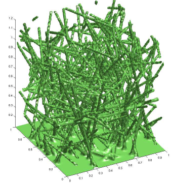
Figure 1: Rendering of an example of the foam surface used in this paper. This foam had 80 fibers of radius 0.01 in a height of 1, giving it $A=10,D=4.3\%,\bar{u}=2.2$ This is a dense foam.

IV Analytic model

To support the numerical results, we formulated an analytic model of secondary electron emission from foam. This analytic model is an extension of a model published in our previous paper swanson2016 . While our previous model considered a field of uniformly aligned whiskers ($\hat{a}=\hat{z}$), we consider a field of randomly aligned whiskers ($\hat{a}$ isotropic). Here, $\hat{a}$ is the direction of the whisker axis.

As in the velvet model, we consider only one generation of secondary electrons. No tertiary electrons will be considered.

As in the velvet model, we will assume that electrons inside a whisker layerl hit the whiskers with uniform probability per unit distance traveled perpendicular to the whiskers’ axes. If the whiskers have radius $r$ and areal density (whiskers per unit area, where area is defined perpendicular to the axis) $n$, the probability of intersection with a whisker is

$$P(hit)=2rndS_{\perp}$$ (3)

where $dS_{\perp}$ is the distance traveled perpendicular to the axis. If the whiskers are aligned along $\hat{a}$, this becomes

$$P(hit)=2rn\frac{\sqrt{1-\hat{v}\cdot\hat{a}^{2}}}{\hat{v}\cdot\hat{z}}dz$$ (4)

where $z$ is the direction normal to the solid surface and $\hat{v}$ is the direction of primary electron incidence. This equation is linear with density $n$ of whiskers. Different populations of whiskers $1,2$ will add:

$$P_{1+2}(hit)=2rn_{1}\frac{\sqrt{1-\hat{v}\cdot\hat{a_{1}}^{2}}}{\hat{v}\cdot\hat{z}}dz+2rn_{2}\frac{\sqrt{1-\hat{v}\cdot\hat{a_{2}}^{2}}}{\hat{v}\cdot\hat{z}}dz$$ (5)

Since $\hat{a}$ is isotropic, $l\equiv\hat{a}\cdot\hat{v}$ is uniformly distributed. Thus in a field of infinitely many infinitesimally dense fields of isotropically aligned whiskers, the probability of hitting one is

$$P(hit)=2rn\frac{dz}{\mu}\int^{1}_{-1}dl\frac{\sqrt{1-l^{2}}}{2}=\frac{\pi}{2}rn\frac{dz}{\mu}$$ (6)

where $\mu\equiv\hat{v}\cdot\hat{z}$.

The probability that an electron will traverse $\Delta z$ without having hit a whisker is this value integrated over $z$

$$P(\Delta z)=e^{-\frac{\pi}{2}rn\frac{\Delta z}{\mu}}=e^{\frac{\bar{u}}{\mu}\frac{\Delta z}{h}}$$ (7)

We have discovered the important parameter to describe the SEY reduction from a foam, $\bar{u}\equiv\frac{\pi}{2}rhn=AD/2$ where $A$ is the aspect ratio $A\equiv h/r$ and $D$ is the volume fill density. $\bar{u}$ is a measure of how much whisker there is: the more dense, or long, or wide the whiskers, the higher $\bar{u}$. It is related ($\bar{u}=\frac{\pi}{4}u$) to the parameter $u$ found for velvet, with the differences in geometry accounting for the numerical coefficient swanson2016 .

The reduction from SEY can be interpreted as the probability that a secondary electron will escape from the whisker layer

$$\gamma_{eff}=\gamma P(escape).$$ (8)

The electrons may be produced either at the top of the foam, at the bottom surface where the foam meets the solid substrate, or on the sides of the whiskers,

$$\gamma_{eff}=\gamma_{top}+\gamma_{bottom}+\gamma_{sides}.$$ (9)

We shall now determine the value of each of these.

If a primary electron hits the top of the foam region, where the foam meets the vacuum, all secondary electrons will be freely conducted to the bulk. A primary electron hits the top with probability $D$, as this is the proportion of the top surface which is taken up by material.

$$\gamma_{top}=D\gamma$$ (10)

The SEY from the bottom surface is:

$$\gamma_{bottom}=\gamma P(escape|bottom)P(bottom)$$ (11)

The probability that a primary electron will make it to the bottom surface is derivable from equation 7.

$$P(bottom)=e^{-\frac{\bar{u}}{\mu}}$$ (12)

The probability that a secondary electron will escape after being emitted from the bottom depends on its emitted polar angle and in integrated form is

$$P(escape|bottom)=\int^{1}_{0}d\mu_{2}P(escape|\mu_{2},bottom)P(\mu_{2})$$ (13)

where $P(\mu_{2})d\mu_{2}$ is the probability density function (PDF) of $\mu_{2}=\cos\theta_{2}$, the polar angle of the secondary electron. Assuming a cosine distribution for the probability of polar angles of secondary electrons Bronstein , $P(\mu_{2})=2\mu_{2}$.

$P(escape|\mu_{2},bottom)$ is also calculable from Equation 7, yielding a final bottom SEY of

$$\gamma_{bottom}=2\gamma(1-D)\int^{1}_{0}d\mu_{2}\mu_{2}e^{-(\frac{1}{\mu}+\frac{1}{\mu_{2}})\bar{u}}$$ (14)

The procedure is similar for $\gamma_{sides}$, except that the secondary electron may be emitted at any $z$ value from 0 to $h$.

$$\gamma_{sides}=\left\langle\gamma\right\rangle(1-D)\int^{h}_{0}dzP(escape|z)P(z)$$ (15)

Again $P(z)dz$, the PDF that an electron hit within $dz$ may be derived from Equation 7.

$\left\langle\gamma\right\rangle$ is necessary as, according to the empirical model of Vaughan vaughan , SEY from a primary electron which is shallowly incident is larger than SEY from a primary electron which is normally incident. According to Equation 2 and the value of $k_{s}=1$ of a smooth surface, the average SEY from isotropically aligned surface elements will be larger than that of the flat value by

$$\left\langle\gamma\right\rangle/\gamma=\int^{1}_{0}d(\cos\theta)2\cos\theta(1+\frac{\theta^{2}}{2\pi})\approx 1.12$$ (16)

Keeping explicit the dependence on $\mu_{2}$, Equation 15 may be written

$$\gamma_{sides}=\left\langle\gamma\right\rangle(1-D)\int^{1}_{0}d\frac{z}{h}\int^{1}_{0}d\mu_{2}\frac{\bar{u}}{\mu}e^{-\bar{u}\frac{z}{h}(\frac{1}{\mu}+\frac{1}{\mu_{2}})}P(\mu_{2}|\mu)$$ (17)

Carrying out the $z$ integration

$$\gamma_{sides}=\left\langle\gamma\right\rangle(1-D)\int^{1}_{0}d\mu_{2}\frac{1-e^{-\bar{u}(\frac{1}{\mu}+\frac{1}{\mu_{2}})}}{1+\frac{\mu}{\mu_{2}}}P(\mu_{2}|\mu)$$ (18)

The function $P(\mu_{2}|\mu)$ is the probability that a primary electron with polar velocity vector component $\mu=\cos\theta$ will produce a secondary electron with polar velocity component $\mu_{2}=\cos\theta_{2}$. Clearly this depends on where on a fiber this electron hits, and how the fiber is aligned.

Here we appeal to geometrical reasoning. Since $\hat{a}$, the whisker axes, are isotropically distributed, so too are $\hat{n}$, the vectors normal to the surface elements on the sides of the whiskers. Because of this, the probability that a primary electron hits a surface element with normal $\hat{n}$ will be linearly weighted by $\hat{v}\cdot\hat{n}$.

Integrating over all surface element normal vectors,

$$P(\mu_{2}|\mu)=\frac{4}{\pi}\int^{1}_{-1}dm(A_{1}\sin\phi_{1}+B_{1}\phi_{1})(A_{2}\sin\phi_{2}+B_{2}\phi_{2})$$ (19)

$$A_{1,2}=\sqrt{(1-m^{2})(1-\mu_{1,2}^{2})},B_{1,2}=m\mu_{1,2}$$

$$\phi_{1,2}=Re[\cos^{-1}(-\frac{B_{1,2}}{A_{1,2}})]$$

where $Re(x)$ is the real part of $x$. $m$ is an integration variable, but it may be informative to know that $m=\hat{n}\cdot\hat{z}$.

Thus the total SEY from a foam surface is expected to be

$$\begin{split}\gamma_{eff}=\gamma D+(1-D)[\gamma\int^{1}_{0}d\mu_{2}2\mu_{2}e^{-(\frac{1}{\mu}+\frac{1}{\mu_{2}})\bar{u}}\\ +\left\langle\gamma\right\rangle\int^{1}_{0}d\mu_{2}\frac{1-e^{-\bar{u}(\frac{1}{\mu}+\frac{1}{\mu_{2}})}}{1+\frac{\mu}{\mu_{2}}}P(\mu_{2}|\mu)]\end{split}$$ (20)

where $\left\langle\gamma\right\rangle$ is defined in Equation 16 and $P(\mu_{2}|\mu)$ is defined in Equation 19. Recall that $\mu=\cos\theta$, where $\theta$ is the polar angle. Also recall that $D$ is the volumetric fill ratio and $\bar{u}=AD/2$ where $A=h/r$ the ratio between the whisker layer thickness and the whisker radius.

The factor in the square brackets is a function only of $\bar{u}$ and $\theta$. It is plotted in Figure 2.

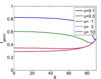
Figure 2: Results of analytic theory. Total SEY is $\gamma[D+(1-D)f_{geom}]$.

For the case of isolated hard-sphere balls of radius $r$, volume density $n$, and layer height $h$, the analytical calculation for SEY is identical. This includes the value of $P(\mu_{2}|\mu)$. For this case,

$$\bar{u}_{ball}=\pi r^{2}nh$$ (21)

V Results and explanantion

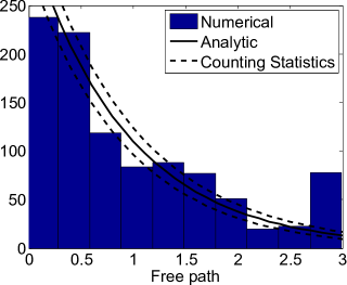
Figure 3: Mean Free Path comparison: A histogram of free paths calculated during a Monte Carlo simulation compared with the idealized analytic version. Error arises from the counting statistics of both particles and whiskers.

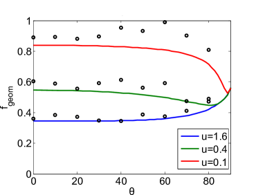
Figure 4: Results of analytic theory compared to full numerical Monte Carlo model.

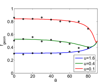
Figure 5: Results of analytic theory compared to simplified Monte Carlo model consisting of only one generation of secondary electrons and no dependence of SEY on primary angle of incidence.

The analytic model is based on the assumption that the mean free path is

$$\lambda_{mfp}=(\frac{\pi}{2}rn)^{-1}$$ (22)

To verify this, we tabulated the free paths of electrons within the foam layer during a Monte Carlo calculation.

The results are plotted in histogram form in Figure 3. For this calculation, whisker parameters were $r=0.005,h=3$, and 160 whiskers were in the simulation volume. This produced a $\bar{u}=3.2$ and a $\lambda_{mfp}=0.94$. The figure indicates that the assumption is qualitatively justified. The excess at a free path of 3 is the result of electrons hitting the bottom surface.

The normalized SEY as a function of primary angle of incidence and the $\bar{u}$ factor is plotted in Figure 4. Three values of $\bar{u}$ are plotted: The $\bar{u}=0.1$ run was initialized with whisker layer height $h=3$, whisker radius $r=0.0025$, and 10 whiskers total in this volume. The $\bar{u}=0.4$ run was initialized with whisker layer height $h=3$, whisker radius $r=0.0025$, and 40 whiskers total in this volume. The $\bar{u}=1.6$ run was initialized with whisker layer height $h=3$, whisker radius $r=0.005$, and 80 whiskers total in this volume.

We can see from Figure 4 that the analytic theory consistently under-estimates the SEY from a given foam by about $10\%$. The source of this discrepancy is subsequent generations of secondary electrons. In the analytic model, only one generation of secondary electrons is considered. In in Figure 5, tertiary electrons are disabled. The numerically and analytically calculated results in Figure 5 are consistent.

The behavior of $\gamma$ at very small $\bar{u}$ can be explained thusly: When there are very few whiskers, or they are very thin, or the whisker layer is very short, the probability of interacting with a whisker is small and so SEY is not reduced by much.

The behavior of $\gamma$ at shallow angles of incidence ($\theta\rightarrow 90^{\circ}$) can be explained simply. A primary electron that is shallowly incident will hit a whisker very close to the top of the whisker layer. Because of isotropy of the whisker axes, this electron will have a 0.5 probability of being emitted with velocity in the upward hemisphere and a 0.5 probability of being emitted with velocty in the downward hemisphere. Thus the SEY from shallow incidence will be reduced by one-half.

The behavior at more normal angles (low $\theta$) at high $\bar{u}$ is very isotropic. There is very little dependence on the angle. This is expected: As $\bar{u}$ increases, almost no electrons penetrate to the bottom surface. If the bottom surface is not relevant, the problem is entirely isotropic. Interestingly, the value of minimum SEY reduction factor is close to $1/e$, the inverse Euler’s constant. This is the value expected from an isotropically scattering and absorbing medium, such as a field of infinitesimal hard spheres.

VI Conclusions

We calcuated the SEY from a foam surface and verified that it is reduced. Furthermore our calculations support the prediction that SEY from a foam surface will behave more isotropically than from other fiberous surfaces like velvet. We find that foam cannot reduce SEY by more than about $30\%$ of its un-suppressed value. We find that foam does not suppress SEY as much as velvet given the same geometric factors $A,D$.

VI.1 Acknowledgment

The authors would like to thank Yevgeny Raitses, who attracted our attention to the SEY of complex surfaces. We would also like to thank Eugene Evans, who suggested the approach of isosurfaces. This work was conducted under a subcontract with UCLA with support of AFOSR under grant FA9550-11-1-0282.

References

- (1) J. R. M. Vaughan, Multipactor, IEEE Trans. Electron Devices 35, 1172-1180 (1988).
- (2) Y. Raitses, et al., “Effect of Secondary Electron Emission on Electron Cross-Filed Current in Discharges,” IEEE Trans. on Plasma Scie. 39, 995 (2011).
- (3) Hongyue Wang, Michael D. Campanell, Igor D. Kaganovich, Guobiao Cai, “Effect of asymmetric secondary emission in bounded low-collisional EB plasma on sheath and plasma properties”, Journal of Physics D: Applied Physics, 47, 405204 (2014).
- (4) Raitses, Y., I. D. Kaganovich, and A. V. Sumant. ”Electron emission from nano-and micro-engineered materials relevant to electric propulsion.” In 33rd International Electric Propulsion Conference, The George Washington University, Washington, DC, USA, pp. 6-10. 2013.
- (5) G. Stupakov and M. Pivi, Suppression of the Effective Secondary Emission Yield for a Grooved Metal Surface, Proc. 31st ICFA Advanced Beam Dynamics Workshop on Electon-Cloud Effects, Napa, CA, USA, April 19-23, 2004.
- (6) L. Wang et al., Suppression of Secondary Electron Emission using Triangular Grooved Surface in the ILC Dipole and Wiggler Magnets, Proc. of Particle Accelerator Conference (PAC 2007), Albuquerque, NM, USA, June 25-29, 2007.
- (7) M. T. F. Pivi et al., “Sharp Reduction of the Secondary Electron Emission Yield from Grooved Surfaces,” J. Appl. Phys. 104, 104904 (2008).
- (8) Y. Suetsugu et al., Experimental Studies on Grooved Surfaces to Suppress Secondary Electron Emission, Proc. IPAC’10, Kyoto, Japan, 2021-2023 (2010).
- (9) D. Ruzic, R. Moore, D. Manos, and S. Cohen Secondary electron yields of carbon-coated and polished stainless steel, J. Vac. Sci. Technol. 20, 1313 (1982).
- (10) V. Baglin, J. Bojko, O. Grabner, B. Henrist, N. Hilleret, C. Scheuerlein, M. Taborelli, The secondary electron yield of technical materials and its variation with surface treatments, Proceedings of EPAC 2000, 26-30 June 2000, Austria Center, Vienna, pp. 217-221.
- (11) Ye, Ming, Wang Dan, and He Yongning. “Mechanism of Total Electron Emission Yield Reduction Using a Micro-Porous Surface.” Journal of Applied Physics 121, no. 12 (March 22, 2017): 124901. doi:10.1063/1.4978760.
- (12) L. Aguilera et al. “CuO Nanowires for Inhibiting Secondary Electron Emission,” J. Phys. D: Appl. Phys. 46, 165104 (2013).
- (13) Huerta, Cesar E., and Richard E. Wirz. Surface Geometry Effects on Secondary Electron Emission Via Monte Carlo Modeling. In 52nd AIAA/SAE/ASEE Joint Propulsion Conference. American Institute of Aeronautics and Astronautics, July 25 2016. http://arc.aiaa.org/doi/abs/10.2514/6.2016-4840.
- (14) Swanson, Charles, and Igor D. Kaganovich. “Modeling of Reduced Effective Secondary Electron Emission Yield from a Velvet Surface.” Journal of Applied Physics 120, no. 21 (December 7, 2016): 213302. doi:10.1063/1.4971337.
- (15) Swanson, Charles, and Igor D. Kaganovich. “ ‘Feathered’ Fractal Surfaces to Minimize Secondary Electron Emission for a Wide Range of Incident Angles.” Journal of Applied Physics 122, no. 4 (July 24, 2017): 043301. doi:10.1063/1.4995535.
- (16) R. Cimino et al., “Search for New e-cloud Mitigator Materials for High Intensity Particle Accelerators,” Proc. of IPAC2014, Dresden, Germany 2332-2334 (2014).
- (17) Patino, M, Y Raitses, and R Wirz. “Secondary Electron Emission from Plasma-Generated Nanostructured Tungsten Fuzz.” Applied Physics Letters 109, no. 20 (November 14, 2016): 201602. doi:10.1063/1.4967830.
- (18) J. Scholtz et al., “Secondary Electron Emission Properties,” Phillips J. Res. 50, 375 (1996).
- (19) I.M. Bronstein, B.S. Fraiman, eds., in “Vtorichnaya Elektronnaya Emissiya”, (Nauka: Movkva), (1969) p. 340 (In Russian)
- (20) M. Patino, Y. Raitses, B. Koel and R. Wirz, Application of Auger Spectroscopy for Measurement of Secondary Electron Emission from Conducting Material for Electric Propulsion Devices, IEPC-2013-320, the 33rd International Electric Propulsion Conference, The George Washington University, Washington, D.C., USA, October 6 - 10, 2013.
- (21) J. Vaughan, “A New Formula for Secondary Emission Yield”, IEEE Trans. on Electron Devices 36, 9 (1989).