Manifold Data Analysis with Applications to High-Frequency 3D Imaging

\nameHyun Bin Kanga,Matthew Reimherra, Mark D. Shriverb, and Peter Claesc CONTACT Hyun Bin Kang. Email: huk163@psu.edu; Matthew Reimherr. Email: mreimherr@psu.edu; Mark D. Shriver. Email: mds17@psu.edu; Peter Claes. Email: peter.claes@kuleuven.be a Department of Statistics, The Pennsylvania State University, University Park, PA, USA;
b Department of Anthropology, The Pennsylvania State University, University Park, PA, USA;
c Department of Electrical Engineering, KU Leuven, Leuven, Belgium
Abstract

Many scientific areas are faced with the challenge of extracting information from large, complex, and highly structured data sets. A great deal of modern statistical work focuses on developing tools for handling such data. This paper presents a new subfield of functional data analysis, FDA, which we call Manifold Data Analysis, or MDA. MDA is concerned with the statistical analysis of samples where one or more variables measured on each unit is a manifold, thus resulting in as many manifolds as we have units. We propose a framework that converts manifolds into functional objects, an efficient 2-step functional principal component method, and a manifold-on-scalar regression model. This work is motivated by an anthropological application involving 3D facial imaging data, which is discussed extensively throughout the paper. The proposed framework is used to understand how individual characteristics, such as age and genetic ancestry, influence the shape of the human face.

keywords:
Functional data analysis; Manifold data analysis; Shape analysis; Manifold learning; Functional principal component analysis; Functional regression

1 Introduction

Functional data analysis, FDA, has seen a precipitous growth in recent years, due in part to the numerous complex data that have have emerged. FDA methods exploit what Ramsay and Silverman (2005) termed replication and regularization. In particular, unlike classic nonparametric smoothing methods, the data usually consist of as many functions as there are statistical units, while the inherent smoothness in the data/parameters can be exploited to achieve greater statistical efficiency than typical multivariate methods (assuming they can even be applied). The present work is concerned with opening a new avenue for functional data methods; a subbranch of FDA we are calling Manifold Data Analysis, MDA. In particular, we present an inferential framework when one of the variables being considered is a manifold, and thus we assume we have as many manifolds as we have units. Our approach utilizes deformation maps from shape analysis and dimension reduction techniques from manifold learning, which allows us to represent each manifold as a Function, which can then be analyzed using FDA techniques. Currently, shape analysis methods that go beyond an analysis of landmarks is a very active area of research; our hope is that building a connection with FDA will open up exciting avenues for both shape and functional data analysis, while providing powerful and flexible statistical tools.

1.1 High-Frequency 3D Facial Imaging

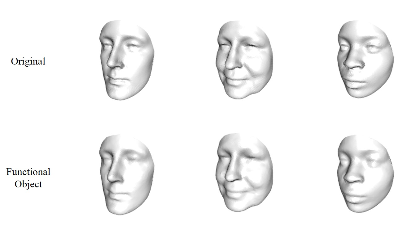
ADAPT (Anthropology, DNA, and the Appearance and Perception of Traits) is an ongoing study at Pennsylvania State University whose aim is to better understand the architecture of human facial diversity using sophisticated biomaging technologies. Investigators of ADAPT collected 3D facial images, alongside genetic information, from admixed populations in the US, Brazil, and Cape Verde (Claes et al., 2014b, a). An anthropometric mask (Claes et al., 2012) with 7150 quasi-landmarks was mapped onto the original 3D images, establishing a spatially-dense correspondences between faces where all facial images have the exact same number of points and sustain anatomical homology across individuals. A generalized Procrustes superimposition (Rohlf and Slice, 1990) was used to scale and align them. The participants also provided basic demographic information including gender, age, height, and weight. A sample of 6564 subjects that have been genotyped is used in the present work. The top three plots in Figure 6 show three examples of the types of facial images that were collected.

There has been extensive research on 3D facial analysis, but the methodologies have been primarily developed in computer science, electrical engineering, and computer vision for face and facial expression recognition (Turk and Pentland, 1991; Ahonen et al., 2006; Jain and Li, 2011; Taigman et al., 2014; Huang et al., 2014b). There is a more limited literature on 3D facial analysis using a statistical framework, and the few existing methods are primarily concerned with classification or estimation based on facial features, not on understanding the influence of different covariates on the 3D faces themselves. Huang et al. (2014a) introduce a local descriptor multi-modal (2D and 3D) for facial gender and ethnicity classification. Xia et al. (2013) adopt machine learning techniques to find relationships between gender and facial asymmetry. Xia et al. (2014) examine age effects using a random forest-based regression, but the regression uses features of local shape deformation between facial curves, captured by Dense Scalar Fields based on Riemannian shape analysis (Drira et al., 2012). Kurtek and Drira (2015) provide a statistical shape analysis framework for 3D faces which allows comparison, deformation, and expression and identity classification, but there has not yet been a corresponding regression method developed that directly takes 3D faces as variables. Porro-Muñoz et al. (2014) attempt to represent faces using splines for face recognition but they do not consider them as manifolds. In contrast, this work proposes a novel functional data approach to analyzing 3D faces, which are viewed as smooth manifolds; by constructing 3D facial functional objects, we can utilize existing functional data analysis tools. Our goal is to build statistical models that elucidate how different covariates affect patterns seen in different faces. However, we do not reduce the faces down to a few quantitative traits, instead we exploit inherently smooth structures in the face so that they can be analyzed as a whole.

1.2 Manifolds in Functional Data Analysis

Functional Data Analysis (Ramsay and Silverman, 2005; Graves et al., 2009; Horváth and Kokoszka, 2012; Kokoszka and Reimherr, 2017) concerns the analysis of data consisting of random functions. It has been used extensively in a variety of fields including geoscience, health studies, kinesiology, and finance to name only a few. In recent years there has been an increased interest in exploring how to apply functional data techniques when working with different types of manifolds. Chen and Müller (2012) consider extending functional data techniques to data that are all lying on a single manifold. Elhamifar and Vidal (2011) consider clusters of functional data with each cluster lying on a different manifold. Ellingson et al. (2013) consider mean estimation from functional data all lying on a common manifold. Dimeglio et al. (2014) also try to find a template function using manifold embedding, considering observed functions as variables with values on a single manifold. Lila et al. (2016) provide a smooth principal component analysis algorithm for functions on a two-dimensional manifold. Ettinger et al. (2016) map the the internal carotid artery on a planar domain, which is also a manifold that is homeomorphic to a cylinder. In previous FDA work, all data is assumed to lie on a single manifold or a small number of manifolds. In this work, however, we assume that each unit is its own manifold, meaning that we have as many manifolds as we have units. High-dimensional 3D imaging is becoming more common in fields such as biology, kinesiology, engineering, and anthropology. In many of these cases, each image is actually a surface sitting in 3D space, i.e. a manifold. However, from image to image, the manifold changes and one cannot assume that all images lie on the same manifold.

1.3 Overview

The remainder of this paper is organized as follows. In Section 2.1 we present an algorithm for converting manifolds into functional objects, while Section 2.2 presents a computationally efficient 2-step Functional Principal Component Analysis (FPCA) algorithm and Section 2.3 introduces a manifold-on-scalar regression model. In Section 4 we apply these methods to the ADAPT data, with Section 4.1 creating facial functional objects, Section 4.2 showing the results of the 2-step FPCA, and Section 4.3 presenting the regression model of gender, age, height, weight, and genetic ancestry on 3D facial functional objects. We conclude the paper with a discussion in Section 5.

2 Methodology

In this section we present our approach for handling random samples of manifolds. Our primary aim is to lay the foundation for analyzing such data using FDA tools. To accomplish this, we use tools from shape analysis so that each manifold can be associated with a particular deformation map, while we use tools from Manifold learning and FDA to carry out the described computations. In Section 2.1 we introduce a statistical framework to embed a sample of manifolds into a real separable Hilbert space, resulting in a sample of functional objects. We then present a computationally efficient 2-step Functional Principal Component Analysis (FPCA) algorithm in Section 2.2. In Section 2.3, we discuss a manifold-on-scalar regression model and hypothesis testing methods for its coefficient functions.

2.1 Algorithm

In order to ensure the manifolds are comparable and that our algorithm can be applied, we make the following assumptions.

Assumption 2.1.

Let 𝒴1,,𝒴Nsubscript𝒴1subscript𝒴𝑁\mathscr{Y}_{1},\cdots,\mathscr{Y}_{N} be a random sample of manifolds. We assume that, with probability one,

  1. 1.

    each 𝒴nsubscript𝒴𝑛\mathscr{Y}_{n} is a compact d-dimensional manifold that is a subset of Dsuperscript𝐷\mathbb{R}^{D} with d<D𝑑𝐷d<D,

  2. 2.

    there exists a nonrandom compact d-dimensional C1superscript𝐶1C^{1} Riemannian manifold 0subscript0\mathcal{M}_{0} such that each 𝒴nsubscript𝒴𝑛\mathscr{Y}_{n} is homeomorphic to 0subscript0\mathcal{M}_{0},

  3. 3.

    there exists an atlas for 0subscript0\mathcal{M}_{0} with a single coordinate chart {(0,ψ)}subscript0𝜓\{(\mathcal{M}_{0},\psi)\} where for any open set U0𝑈subscript0U\subset\mathcal{M}_{0}, ψ:Uψ(U)d:𝜓𝑈𝜓𝑈superscript𝑑\psi:U\rightarrow\psi(U)\subset\mathbb{R}^{d} and 𝐌0ψ(0)subscript𝐌0𝜓subscript0{\bf M}_{0}\triangleq\psi(\mathcal{M}_{0}),

  4. 4.

    to each manifold 𝒴nsubscript𝒴𝑛\mathscr{Y}_{n}, there exists a function 𝐘n:𝐌0D:subscript𝐘𝑛subscript𝐌0superscript𝐷{\bf Y}_{n}:{\bf M}_{0}\rightarrow\mathbb{R}^{D} such that 𝐘n(𝐌0)=𝒴nsubscript𝐘𝑛subscript𝐌0subscript𝒴𝑛{\bf Y}_{n}({\bf M}_{0})=\mathscr{Y}_{n}, up to possibly a set of measure 0,

  5. 5.

    the functions 𝐘nsubscript𝐘𝑛{\bf Y}_{n} are elements of L2(𝐌0)superscript𝐿2subscript𝐌0L^{2}({\bf M}_{0}) with probability one, i.e. 𝐌0𝐘n(m)𝐘n(m)𝑑m<subscriptsubscript𝐌0superscriptsubscript𝐘𝑛top𝑚subscript𝐘𝑛𝑚differential-d𝑚\int_{{\bf M}_{0}}{\bf Y}_{n}^{\top}(m){\bf Y}_{n}(m)dm<\infty.

The first assumption states that the sample consists of manifolds that are in the same ambient space, Dsuperscript𝐷\mathbb{R}^{D}. This can be generalized to other spaces, but we do not pursue that here given the scope of our intended applications. The second guarantees that the manifolds are comparable by assuming that they can all be parametrized by a common manifold, 0subscript0\mathcal{M}_{0}. This manifold is assumed to be C1superscript𝐶1C^{1} and Riemannian so that integration over the manifold is well defined (Lee, 2003). The third assumption lets us apply manifold learning methods to “unfold” 0subscript0\mathcal{M}_{0} into the simpler set 𝐌0subscript𝐌0{\bf M}_{0}. This is primarily for computational convenience, as 𝐌0subscript𝐌0{\bf M}_{0} is a an easier domain to work with. If the third assumption does not hold, then the manifold, 0subscript0{\mathcal{M}}_{0}, cannot be mapped to a set in dsuperscript𝑑{\mathbb{R}}^{d} without tearing it in some way. Such an assumption is reasonable for our facial applications, but, for example Ettinger et al. (2016) utilize FDA methods for data measured on the internal carotid atrtery, which is homeomorphic to a cylinder and thus would violate this assumption. We discuss this further in Section 5. The fourth assumption simply allows us to identify the manifolds as functions, which are commonly referred to as deformation maps in shape analysis , while the fifth assumption allows us to view those functions as elements of a Hilbert space.

At the heart of our methodology is the view that each manifold can be identified with a function, and then properties such as smoothness can be defined and exploited by utilizing these functions. The major difference between our setting and traditional FDA is that the domain, 𝐌0subscript𝐌0{\bf M}_{0}, is not observed and must therefore be constructed. Furthermore, it is assumed that the data are smooth with respect to distance along 0subscript0\mathcal{M}_{0}, not along Dsuperscript𝐷\mathbb{R}^{D}. The framework to construct 𝐘n:𝐌0D:subscript𝐘𝑛subscript𝐌0superscript𝐷{\bf Y}_{n}:{\bf M}_{0}\rightarrow\mathbb{R}^{D} from 𝒴nsubscript𝒴𝑛\mathscr{Y}_{n} is summarized below.

  1. 1.

    Identify a reference manifold 0subscript0\mathcal{M}_{0}.

  2. 2.

    Embed 0subscript0\mathcal{M}_{0} into a closed bounded connected region of dsuperscript𝑑\mathbb{R}^{d} to construct 𝐌0subscript𝐌0{\bf M}_{0}.

  3. 3.

    Align 𝒴nsubscript𝒴𝑛\mathscr{Y}_{n} to 0subscript0\mathcal{M}_{0} and thus also to 𝐌0subscript𝐌0{\bf M}_{0}.

  4. 4.

    Construct basis functions from 𝐌0subscript𝐌0{\bf M}_{0} to Dsuperscript𝐷\mathbb{R}^{D} and express 𝐘nsubscript𝐘𝑛{\bf Y}_{n} as a linear combination of these functions.

We now discuss each of the steps above. We assume that the raw data is of the form {ynpq:n=1,,N;p=1,,P;q=1,,D}conditional-setsubscripty𝑛𝑝𝑞formulae-sequence𝑛1𝑁formulae-sequence𝑝1𝑃𝑞1𝐷\{\mathrm{y}_{npq}:n=1,\cdots,N;p=1,\cdots,P;q=1,\cdots,D\}, which consists of P𝑃P D𝐷D-dimensional points observed on manifolds 𝒴1,,𝒴Nsubscript𝒴1subscript𝒴𝑁\mathscr{Y}_{1},\cdots,\mathscr{Y}_{N}. We assume that each manifold is ultra-densely sampled, and thus can be completely reconstructed with almost no error, which is a common assumption Dense Functional Data Analysis (Zhang and Wang, 2016).

For the first step, the reference manifold 0subscript0\mathcal{M}_{0} can be taken from an external source, such as previous literature or a previously constructed library of objects, one of the manifolds in the sample, or an average from the sample. This choice of 0subscript0\mathcal{M}_{0} is closely related to second and third step, so it needs to be chosen carefully.

Once 0subscript0\mathcal{M}_{0} is identified, we use manifold learning techniques on 0subscript0\mathcal{M}_{0} to find 𝐌0subscript𝐌0{\bf M}_{0}, the embedding of 0subscript0\mathcal{M}_{0} in to dsuperscript𝑑\mathbb{R}^{d}. The resulting points will be denoted as {mpq:p=1,,P;q=1,,d}conditional-setsubscriptm𝑝𝑞formulae-sequence𝑝1𝑃𝑞1𝑑\{\mathrm{m}_{pq}:p=1,\cdots,P;q=1,\cdots,d\}, P𝑃P. Manifold learning has been a very active area of research, and there are a number of popular methods for carrying out this step, including Isomap (Tenenbaum et al., 2000), Laplacian Eigenmaps (Belkin and Niyogi, 2003), local linear embedding (Saul and Roweis, 2003, LLE), local tangent space alignment (Zhang and Zha, 2004, LTSA), and Diffusion Map (Nadler et al., 2006). All of these methods aim to find a low-dimensional representation of the given data, but they utilize different strategies towards achieving it. Isomap finds a lower-dimensional embedding that best preserves the geodesic distance between all points, while Laplacian Eigenmaps tries to preserve local distances. LLE seeks to maintain neighborhood distances. LTSA is algorithmically similar to LLE but tries to learn local neighborhood geometry via tangent spaces and aligns them to find the underlying manifold. Diffusion map uses a different perspective by considering a random walk “diffusing” through the points, and uses a particular eigendecomposition related to that walk to obtain the low dimensional embedding. Spanifold (Chenouri et al., 2015) sets up a tree on the manifold and tries to maintain pairwise distance relationships within the tree while flattening the manifold. In section 4.1 we will compare the performance of these different approaches on the ADAPT data.

We align all 𝒴1,,𝒴Nsubscript𝒴1subscript𝒴𝑁\mathscr{Y}_{1},\cdots,\mathscr{Y}_{N} to the reference manifold 0subscript0\mathcal{M}_{0}. In other words, we find a representation of 𝒴nsubscript𝒴𝑛\mathscr{Y}_{n} as {y~npq:n=1,,N;p=1,,P;q=1,,D}conditional-setsubscript~y𝑛𝑝𝑞formulae-sequence𝑛1𝑁formulae-sequence𝑝1𝑃𝑞1𝐷\{\tilde{\mathrm{y}}_{npq}:n=1,\cdots,N;p=1,\cdots,P;q=1,\cdots,D\} where {y~npq}subscript~y𝑛𝑝𝑞\{\tilde{\mathrm{y}}_{npq}\} are {ynpq}subscripty𝑛𝑝𝑞\{\mathrm{y}_{npq}\} aligned to 0subscript0\mathcal{M}_{0}. We assume that 𝒴nsubscript𝒴𝑛\mathscr{Y}_{n} is homeomorphic to 0subscript0{\mathcal{M}}_{0} and thus to 𝐌0subscript𝐌0{\bf M}_{0}, which allows us to use 𝐌0subscript𝐌0{\bf M}_{0} as a common domain for 𝒴1,,𝒴Nsubscript𝒴1subscript𝒴𝑁\mathscr{Y}_{1},\cdots,\mathscr{Y}_{N}. For this manifold alignment problem, we rely on shape analysis tools such as Procrustes Analysis (Mardia et al., 1979).

Once the domain, 𝐌0subscript𝐌0{\bf M}_{0}, is calculated, the next step is to construct 𝐘n:𝐌0D:subscript𝐘𝑛subscript𝐌0superscript𝐷{\bf Y}_{n}:{\bf M}_{0}\rightarrow\mathbb{R}^{D} from 𝒴nsubscript𝒴𝑛\mathscr{Y}_{n}. As functional data are commonly expressed with basis functions, we fix basis functions 𝐞j:𝐌0D:subscript𝐞𝑗subscript𝐌0superscript𝐷{\bf e}_{j}:{\bf M}_{0}\rightarrow\mathbb{R}^{D} and then we express the manifolds in functional data format as

𝒴n𝐘n(m)j=1Jbnj𝐞j(m)m𝐌0,formulae-sequencesubscript𝒴𝑛subscript𝐘𝑛𝑚superscriptsubscript𝑗1𝐽subscript𝑏𝑛𝑗subscript𝐞𝑗𝑚𝑚subscript𝐌0\mathscr{Y}_{n}\equiv{\bf Y}_{n}(m)\approx\sum_{j=1}^{J}b_{nj}{\bf e}_{j}(m)\quad\quad m\in{\bf M}_{0},

where bnjsubscript𝑏𝑛𝑗b_{nj}\in\mathbb{R}. The b^njsubscript^𝑏𝑛𝑗\hat{b}_{nj} can be found by minimizing

p=1P|y~np𝐘nJ(mp)|2+λ𝐌0[L(𝐘nJ)(m)]2𝑑msuperscriptsubscript𝑝1𝑃superscriptsubscript~y𝑛𝑝superscriptsubscript𝐘𝑛𝐽subscript𝑚𝑝2𝜆subscriptsubscript𝐌0superscriptdelimited-[]𝐿superscriptsubscript𝐘𝑛𝐽𝑚2differential-d𝑚\displaystyle\sum_{p=1}^{P}|\tilde{{\bf\mathrm{y}}}_{np}-{\bf Y}_{n}^{J}(m_{p})|^{2}+\lambda\int_{{\bf M}_{0}}[L({\bf Y}_{n}^{J})(m)]^{2}dm (1)

where y~np=(y~np1,,y~npD)subscript~y𝑛𝑝superscriptsubscript~y𝑛𝑝1subscript~y𝑛𝑝𝐷top\tilde{{\bf\mathrm{y}}}_{np}=(\tilde{\mathrm{y}}_{np1},\cdots,\tilde{\mathrm{y}}_{npD})^{\top}, 𝐘nJ(m)=j=1Jbnj𝐞j(m)superscriptsubscript𝐘𝑛𝐽𝑚superscriptsubscript𝑗1𝐽subscript𝑏𝑛𝑗subscript𝐞𝑗𝑚{\bf Y}_{n}^{J}(m)=\sum_{j=1}^{J}b_{nj}{\bf e}_{j}(m), and L𝐿L is a linear differential operator. The resulting functional data would be

𝐘n(m)j=1Jb^nj𝐞j(m).subscript𝐘𝑛𝑚superscriptsubscript𝑗1𝐽subscript^𝑏𝑛𝑗subscript𝐞𝑗𝑚{\bf Y}_{n}(m)\approx\sum_{j=1}^{J}\hat{b}_{nj}{\bf e}_{j}(m). (2)

In the ADAPT application we utilize felsplines (Ramsay, 2002) and expand each coordinate, Ynj(m)subscript𝑌𝑛𝑗𝑚Y_{nj}(m), separately, though other approaches including thin plate splines could also be used.

2.2 2-Step Functional Principal Component Analysis

We now introduce a 2-step functional principal component analysis (FPCA) method to be carried out on the objects define in (2). In the first step, we conduct FPCA on the pooled (across the D𝐷D coordinates) sample to reduce the number of basis functions and make them orthogonal. In the second step, we conduct PCA on the resulting array to get eigenvalues λksubscript𝜆𝑘\lambda_{k} and eigenfunctions 𝐕k(m)subscript𝐕𝑘𝑚{\bf V}_{k}(m). Computational tools for basis functions that map a set in lower dimension 𝐌0dsubscript𝐌0superscript𝑑{\bf M}_{0}\in\mathbb{R}^{d} to higher dimension, Dsuperscript𝐷\mathbb{R}^{D}, are currently limited. Therefore, we start with expanding each coordinate of 𝐘nsubscript𝐘𝑛{\bf Y}_{n} using basis functions {ej:𝐌0}conditional-setsubscript𝑒𝑗subscript𝐌0\{e_{j}:{\bf M}_{0}\rightarrow\mathbb{R}\}, and then obtain eigenfunctions 𝐕k:𝐌0D:subscript𝐕𝑘subscript𝐌0superscript𝐷{\bf V}_{k}:{\bf M}_{0}\rightarrow\mathbb{R}^{D} in the second step.

The raw data, {ynpq}subscripty𝑛𝑝𝑞\{\mathrm{y}_{npq}\}, is assumed to be an N×P×D𝑁𝑃𝐷N\times P\times D array, while the basis coefficients from (2) form an N×J×D𝑁𝐽𝐷N\times J\times D array. Our second step consists of tensor multiplication and singular value decompositions, which are substantial computational burdens. Decreasing the dimension by lowering the number of basis functions through the first step lessens the computational time substantially. The burden of the second step is also decreased substantially by exploiting the orthonormal structure of the bases from the first step.

Step 1.

Without loss of generality, assume that the 𝐘n(m)subscript𝐘𝑛𝑚{\bf Y}_{n}(m) have been centered and thus have mean zero. Each of the functions is expressed as

𝐘n(m)=[Yn1(m),,YnD(m)][j=1Jb^nj1ej(m),,j=1Jb^njDej(m)],subscript𝐘𝑛𝑚superscriptsubscript𝑌𝑛1𝑚subscript𝑌𝑛𝐷𝑚topsuperscriptsuperscriptsubscript𝑗1𝐽subscript^𝑏𝑛𝑗1subscript𝑒𝑗𝑚superscriptsubscript𝑗1𝐽subscript^𝑏𝑛𝑗𝐷subscript𝑒𝑗𝑚top{\bf Y}_{n}(m)=\left[Y_{n1}(m),\cdots,Y_{nD}(m)\right]^{\top}\approx\left[\sum_{j=1}^{J}\hat{b}_{nj1}e_{j}(m),\cdots,\sum_{j=1}^{J}\hat{b}_{njD}e_{j}(m)\right]^{\top},

for n=1,,N𝑛1𝑁n=1,\dots,N. We stack all of the coordinate-wise functions into a single vector of functions with dimension ND𝑁𝐷ND. We denote the resulting functions as Yl(m)subscript𝑌𝑙𝑚Y_{l}(m) where Yl(m)=Ynq(m)subscript𝑌𝑙𝑚subscript𝑌𝑛𝑞𝑚Y_{l}(m)=Y_{nq}(m) for l=N(q1)+n𝑙𝑁𝑞1𝑛l=N(q-1)+n and n=1,,N𝑛1𝑁n=1,\cdots,N, q=1,,D𝑞1𝐷q=1,\cdots,D.

We find the pairs of eigenvalues ηhsubscript𝜂\eta_{h} and principal component functions ψh:𝐌0D:subscript𝜓subscript𝐌0superscript𝐷\psi_{h}:{\bf M}_{0}\to{\mathbb{R}}^{D}, for h=1,,H1𝐻h=1,\dots,H, which satisfy

ηhψh(m)=𝚽(m,m)ψh(m)𝑑m,subscript𝜂subscript𝜓𝑚𝚽𝑚superscript𝑚subscript𝜓superscript𝑚differential-dsuperscript𝑚\displaystyle\eta_{h}\psi_{h}(m)=\int\mbox{\boldmath${\Phi}$}(m,m^{\prime})\psi_{h}(m^{\prime})dm^{\prime}, (3)
ψh=1,normsubscript𝜓1\displaystyle\|\psi_{h}\|=1, (4)

where

𝚽(m,m)=E[Yl(m)Yl(m)]=j1Jj2JE[blj1blj2]ej1(m)ej2(m)=j1Jj2JΠj1,j2ej1(m)ej2(m).𝚽𝑚superscript𝑚𝐸delimited-[]subscript𝑌𝑙𝑚subscript𝑌𝑙superscriptsuperscript𝑚topsuperscriptsubscriptsubscript𝑗1𝐽superscriptsubscriptsubscript𝑗2𝐽𝐸delimited-[]subscript𝑏𝑙subscript𝑗1subscript𝑏𝑙subscript𝑗2subscript𝑒subscript𝑗1𝑚subscript𝑒subscript𝑗2superscriptsuperscript𝑚topsuperscriptsubscriptsubscript𝑗1𝐽superscriptsubscriptsubscript𝑗2𝐽subscriptΠsubscript𝑗1subscript𝑗2subscript𝑒subscript𝑗1𝑚subscript𝑒subscript𝑗2superscriptsuperscript𝑚top\mbox{\boldmath${\Phi}$}(m,m^{\prime})=E[Y_{l}(m)Y_{l}(m^{\prime})^{\top}]=\sum_{j_{1}}^{J}\sum_{j_{2}}^{J}E[b_{lj_{1}}b_{lj_{2}}]e_{j_{1}}(m)e_{j_{2}}(m^{\prime})^{\top}=\sum_{j_{1}}^{J}\sum_{j_{2}}^{J}\Pi_{j_{1},j_{2}}e_{j_{1}}(m)e_{j_{2}}(m^{\prime})^{\top}.

By expanding ψhsubscript𝜓\psi_{h} using ejsubscript𝑒𝑗e_{j}, ψh(m)=j=1Jwhjej(m)subscript𝜓𝑚superscriptsubscript𝑗1𝐽subscript𝑤𝑗subscript𝑒𝑗𝑚\psi_{h}(m)=\sum_{j=1}^{J}w_{hj}e_{j}(m), equations 3 and 4 become

ηhj=1Jwhjej(m)=j1Jj2Jj3JΠj1,j2𝐙j2,j3ej1(m),subscript𝜂superscriptsubscript𝑗1𝐽subscript𝑤𝑗subscript𝑒𝑗𝑚superscriptsubscriptsubscript𝑗1𝐽superscriptsubscriptsubscript𝑗2𝐽superscriptsubscriptsubscript𝑗3𝐽subscriptΠsubscript𝑗1subscript𝑗2subscript𝐙subscript𝑗2subscript𝑗3subscript𝑒subscript𝑗1𝑚\displaystyle\eta_{h}\sum_{j=1}^{J}w_{hj}e_{j}(m)=\sum_{j_{1}}^{J}\sum_{j_{2}}^{J}\sum_{j_{3}}^{J}\Pi_{j_{1},j_{2}}{\bf Z}_{j_{2},j_{3}}e_{j_{1}}(m),
andj1=1Jj2=1Jwhj1whj2𝐙j1,j2=1,andsuperscriptsubscriptsubscript𝑗11𝐽superscriptsubscriptsubscript𝑗21𝐽subscript𝑤subscript𝑗1subscript𝑤subscript𝑗2subscript𝐙subscript𝑗1subscript𝑗21\displaystyle\text{and}\qquad\sum_{j_{1}=1}^{J}\sum_{j_{2}=1}^{J}w_{hj_{1}}w_{hj_{2}}{\bf Z}_{j_{1},j_{2}}=1,

where 𝐙j1,j2=𝐌0ej1(m)ej2(m)𝑑msubscript𝐙subscript𝑗1subscript𝑗2subscriptsubscript𝐌0subscript𝑒subscript𝑗1superscript𝑚subscript𝑒subscript𝑗2superscript𝑚differential-dsuperscript𝑚{\bf Z}_{j_{1},j_{2}}=\int_{{\bf M}_{0}}e_{j_{1}}(m^{\prime})e_{j_{2}}(m^{\prime})dm^{\prime}. By factoring the matrix 𝐙=𝐆𝐆𝐙superscript𝐆top𝐆{\bf Z}={\bf G}^{\top}{\bf G} and defining ahj=j1=1Jwhj1𝐆jj1subscript𝑎𝑗superscriptsubscriptsubscript𝑗11𝐽subscript𝑤subscript𝑗1subscript𝐆𝑗subscript𝑗1a_{hj}=\sum_{j_{1}=1}^{J}w_{hj_{1}}{\bf G}_{jj_{1}}, we obtain the relations

ηhahj=j2JΠ~j,j2ahj2andj=1Jahj2=1,formulae-sequencesubscript𝜂subscript𝑎𝑗superscriptsubscriptsubscript𝑗2𝐽subscript~Π𝑗subscript𝑗2subscript𝑎subscript𝑗2andsuperscriptsubscript𝑗1𝐽superscriptsubscript𝑎𝑗21\displaystyle\eta_{h}a_{hj}=\sum_{j_{2}}^{J}\tilde{\Pi}_{j,j_{2}}a_{hj_{2}}\qquad\text{and}\qquad\sum_{j=1}^{J}a_{hj}^{2}=1,

where Π~j,j2=j1Jj3J𝐆j,j1Πj1j3𝐆j3j2subscript~Π𝑗subscript𝑗2superscriptsubscriptsubscript𝑗1𝐽superscriptsubscriptsubscript𝑗3𝐽subscript𝐆𝑗subscript𝑗1subscriptΠsubscript𝑗1subscript𝑗3subscript𝐆subscript𝑗3subscript𝑗2\tilde{\Pi}_{j,j_{2}}=\sum_{j_{1}}^{J}\sum_{j_{3}}^{J}{\bf G}_{j,j_{1}}\Pi_{j_{1}j_{3}}{\bf G}_{j_{3}j_{2}}. Further details can be found in the supplementary material. The vector 𝐚j={ahj}subscript𝐚𝑗subscript𝑎𝑗{\bf a}_{j}=\{a_{hj}\} is the jthsuperscript𝑗𝑡j^{th} eigenvector of the covariance matrix Π~~Π\tilde{\Pi}. Using this, we can get

ψh(m)=j=1Jahjej(m).subscript𝜓𝑚superscriptsubscript𝑗1𝐽subscript𝑎𝑗subscript𝑒𝑗𝑚\psi_{h}(m)=\sum_{j=1}^{J}a_{hj}e_{j}(m).

Step 2.

We now expand Ynq(m)subscript𝑌𝑛𝑞𝑚Y_{nq}(m) using the {ψh(m)}subscript𝜓𝑚\{\psi_{h}(m)\}:

Ynq(m)=h=1Hcnhqψh(m).subscript𝑌𝑛𝑞𝑚superscriptsubscript1𝐻subscript𝑐𝑛𝑞subscript𝜓𝑚Y_{nq}(m)=\sum_{h=1}^{H}c_{nhq}\psi_{h}(m).

The coefficients 𝐜={cnhq}𝐜subscript𝑐𝑛𝑞{\bf c}=\{c_{nhq}\} form an N×H×D𝑁𝐻𝐷N\times H\times D array. The covariance operator of 𝐘n(m)subscript𝐘𝑛𝑚{\bf Y}_{n}(m) is given by

Γq,q(m,m)=E[Ynq(m)Ynq(m)]=h1=1Hh2=1HΣh1qh2qψh1(m)ψh2(m)subscriptΓ𝑞superscript𝑞𝑚superscript𝑚𝐸delimited-[]subscript𝑌𝑛𝑞𝑚subscript𝑌𝑛superscript𝑞superscript𝑚superscriptsubscriptsubscript11𝐻superscriptsubscriptsubscript21𝐻subscriptΣsubscript1𝑞subscript2superscript𝑞subscript𝜓subscript1𝑚subscript𝜓subscript2superscript𝑚\Gamma_{q,q^{\prime}}(m,m^{\prime})=E[Y_{nq}(m)Y_{nq^{\prime}}(m^{\prime})]=\sum_{h_{1}=1}^{H}\sum_{h_{2}=1}^{H}\Sigma_{h_{1}qh_{2}q^{\prime}}\psi_{h_{1}}(m)\psi_{h_{2}}(m^{\prime})

with Σh1qh2q=E[cnh1qcnh2q].subscriptΣsubscript1𝑞subscript2superscript𝑞𝐸delimited-[]subscript𝑐𝑛subscript1𝑞superscriptsubscript𝑐𝑛subscript2superscript𝑞top\Sigma_{h_{1}qh_{2}q^{\prime}}=E[c_{nh_{1}q}c_{nh_{2}q^{\prime}}^{\top}]. Now we find the pairs of eigenvalues λksubscript𝜆𝑘\lambda_{k} and eigenfunctions 𝐕k(m)subscript𝐕𝑘𝑚{\bf V}_{k}(m) that satisfy

λk𝐕k(m)=𝚪(m,m)𝐕k(m)𝑑m,subscript𝜆𝑘subscript𝐕𝑘𝑚𝚪𝑚superscript𝑚subscript𝐕𝑘superscript𝑚differential-dsuperscript𝑚\displaystyle\lambda_{k}{\bf V}_{k}(m)=\int\mbox{\boldmath${\Gamma}$}(m,m^{\prime}){\bf V}_{k}(m^{\prime})dm^{\prime}, (5)
𝐕k=1.normsubscript𝐕𝑘1\displaystyle\|{\bf V}_{k}\|=1. (6)

We expand 𝐕ksubscript𝐕𝑘{\bf V}_{k} using the ψhsubscript𝜓\psi_{h} as well:

Vkq(m)=h=1Hvkhqψh(m),subscript𝑉𝑘𝑞𝑚superscriptsubscript1𝐻subscript𝑣𝑘𝑞subscript𝜓𝑚V_{kq}(m)=\sum_{h=1}^{H}v_{khq}\psi_{h}(m),

where 𝐯={vkhq}𝐯subscript𝑣𝑘𝑞{\bf v}=\{v_{khq}\} is a K×H×D𝐾𝐻𝐷K\times H\times D array of coefficients. Since ψhsubscript𝜓\psi_{h} are orthonormal, after several expansions, which are given in the supplementary material, equations 5 and 6 become

λkvkhq=q=1Dh2=1HΣhqh2qvkh2qandq=1Dh1=1Hh2=1Hvkh1qvkh2q=1.formulae-sequencesubscript𝜆𝑘subscript𝑣𝑘𝑞superscriptsubscriptsuperscript𝑞1𝐷superscriptsubscriptsubscript21𝐻subscriptΣ𝑞subscript2superscript𝑞subscript𝑣𝑘subscript2superscript𝑞andsuperscriptsubscript𝑞1𝐷superscriptsubscriptsubscript11𝐻superscriptsubscriptsubscript21𝐻subscript𝑣𝑘subscript1𝑞subscript𝑣𝑘subscript2𝑞1\displaystyle\lambda_{k}v_{khq}=\sum_{q^{\prime}=1}^{D}\sum_{h_{2}=1}^{H}\Sigma_{hqh_{2}q^{\prime}}v_{kh_{2}q^{\prime}}\qquad\text{and}\qquad\sum_{q=1}^{D}\sum_{h_{1}=1}^{H}\sum_{h_{2}=1}^{H}v_{kh_{1}q}v_{kh_{2}q}=1.

So we have that 𝐯k={vkhq}subscript𝐯𝑘subscript𝑣𝑘𝑞{\bf v}_{k}=\{v_{khq}\} for equation 2.2 is the kthsuperscript𝑘𝑡k^{th} eigenmatrix of the H×D×H×D𝐻𝐷𝐻𝐷H\times D\times H\times D covariance tensor ΣΣ\Sigma.

2.3 Manifold-on-Scalar Regression

We now give a Manifold-on-scalar regression strategy by using the functional manifold objects as responses and using scalar predictors, very similar to Function-on-Scalar Regression (Ramsay and Silverman, 2005). The model is given by

𝐘n(m)=xn1𝜷1(m)+xn2𝜷2(m)++xnR𝜷R(m)+𝜺n(m),subscript𝐘𝑛𝑚subscript𝑥𝑛1subscript𝜷1𝑚subscript𝑥𝑛2subscript𝜷2𝑚subscript𝑥𝑛𝑅subscript𝜷𝑅𝑚subscript𝜺𝑛𝑚{\bf Y}_{n}(m)=x_{n1}\mbox{\boldmath${\beta}$}_{1}(m)+x_{n2}\mbox{\boldmath${\beta}$}_{2}(m)+\cdots+x_{nR}\mbox{\boldmath${\beta}$}_{R}(m)+\mbox{\boldmath${\varepsilon}$}_{n}(m), (7)

where there are R𝑅R predictors for every manifold. Recall that 𝐘nsubscript𝐘𝑛{\bf Y}_{n} is the deformation map associated with the manifold, 𝒴nsubscript𝒴𝑛\mathcal{Y}_{n}. Define the terms

𝐘(m)=[𝐘1(m)𝐘2(m)𝐘N(m)],𝐗=[x11x12x1Rx21x22x2RxN1xN2xNR],formulae-sequence𝐘𝑚delimited-[]matrixsubscriptsuperscript𝐘top1𝑚subscriptsuperscript𝐘top2𝑚subscriptsuperscript𝐘top𝑁𝑚𝐗delimited-[]matrixsubscript𝑥11subscript𝑥12subscript𝑥1𝑅subscript𝑥21subscript𝑥22subscript𝑥2𝑅subscript𝑥𝑁1subscript𝑥𝑁2subscript𝑥𝑁𝑅\displaystyle{\bf Y}(m)=\left[\begin{matrix}{\bf Y}^{\top}_{1}(m)\\ {\bf Y}^{\top}_{2}(m)\\ \vdots\\ {\bf Y}^{\top}_{N}(m)\end{matrix}\right],\quad{\bf X}=\left[\begin{matrix}x_{11}&x_{12}&\cdots&x_{1R}\\ x_{21}&x_{22}&\cdots&x_{2R}\\ \vdots&\vdots&\vdots&\vdots\\ x_{N1}&x_{N2}&\cdots&x_{NR}\end{matrix}\right],
𝜷(m)=[𝜷1(m)𝜷2(m)𝜷R(m)],𝜺(m)=[𝜺1(m)𝜺2(m)𝜺N(m)],formulae-sequence𝜷𝑚delimited-[]matrixsubscriptsuperscript𝜷top1𝑚subscriptsuperscript𝜷top2𝑚subscriptsuperscript𝜷top𝑅𝑚𝜺𝑚delimited-[]matrixsubscriptsuperscript𝜺top1𝑚subscriptsuperscript𝜺top2𝑚subscriptsuperscript𝜺top𝑁𝑚\displaystyle{\mbox{\boldmath${\beta}$}}(m)=\left[\begin{matrix}\mbox{\boldmath${\beta}$}^{\top}_{1}(m)\\ \mbox{\boldmath${\beta}$}^{\top}_{2}(m)\\ \vdots\\ \mbox{\boldmath${\beta}$}^{\top}_{R}(m)\end{matrix}\right],\quad{\mbox{\boldmath${\varepsilon}$}}(m)=\left[\begin{matrix}\mbox{\boldmath${\varepsilon}$}^{\top}_{1}(m)\\ \mbox{\boldmath${\varepsilon}$}^{\top}_{2}(m)\\ \vdots\\ \mbox{\boldmath${\varepsilon}$}^{\top}_{N}(m)\end{matrix}\right],

then equation 7 can be expressed as

𝐘(m)=𝐗𝜷(m)+𝜺(m).𝐘𝑚𝐗𝜷𝑚𝜺𝑚{\bf Y}(m)={\bf X}\boldsymbol{\beta}(m)+\mbox{\boldmath${\varepsilon}$}(m).

The least square estimator of the functional parameter 𝜷(m)𝜷𝑚\boldsymbol{\beta}(m) can be found by minimizing

n=1N𝐘nr=1Rxnr𝜷r2=𝐌0n=1N|𝐘n(m)r=1Rxnr𝜷r(m)|2dmsuperscriptsubscript𝑛1𝑁superscriptnormsubscript𝐘𝑛superscriptsubscript𝑟1𝑅subscript𝑥𝑛𝑟subscript𝜷𝑟2subscriptsubscript𝐌0superscriptsubscript𝑛1𝑁superscriptsubscript𝐘𝑛𝑚superscriptsubscript𝑟1𝑅subscript𝑥𝑛𝑟subscript𝜷𝑟𝑚2𝑑𝑚\sum_{n=1}^{N}\left\|{\bf Y}_{n}-\sum_{r=1}^{R}x_{nr}\mbox{\boldmath${\beta}$}_{r}\right\|^{2}=\int_{{\bf M}_{0}}\sum_{n=1}^{N}\left|{\bf Y}_{n}(m)-\sum_{r=1}^{R}x_{nr}\mbox{\boldmath${\beta}$}_{r}(m)\right|^{2}dm (8)

For each fixed m𝑚m, 𝐌0n=1Nen2(𝜷,m)dmsubscriptsubscript𝐌0superscriptsubscript𝑛1𝑁superscriptsubscript𝑒𝑛2𝜷𝑚𝑑𝑚\int_{{\bf M}_{0}}\sum_{n=1}^{N}e_{n}^{2}(\boldsymbol{\beta},m)dm is minimized if

𝜷^(m)=(𝐗𝐗)1𝐗𝐘(m).bold-^𝜷𝑚superscriptsuperscript𝐗top𝐗1superscript𝐗top𝐘𝑚\boldsymbol{\hat{\beta}}(m)=({\bf X}^{\top}{\bf X})^{-1}{\bf X}^{\top}{\bf Y}(m). (9)

We expand 𝐘n(m)subscript𝐘𝑛𝑚{\bf Y}_{n}(m) using functional principal components, 𝐕k(m)3subscript𝐕𝑘𝑚superscript3{\bf V}_{k}(m)\in\mathbb{R}^{3}, from Section 2.2:

𝐘(m)=k=1Kynk𝐕k(m).𝐘𝑚superscriptsubscript𝑘1𝐾subscript𝑦𝑛𝑘subscript𝐕𝑘𝑚{\bf Y}(m)=\sum_{k=1}^{K}y_{nk}{\bf V}_{k}(m).

Let

𝐘(m)=[y11y12y1Ky21y22y2KyN1yN2yNK][𝐕1(m)𝐕2(m)𝐕K(m)]𝐲𝐕(m).𝐘𝑚delimited-[]matrixsubscript𝑦11subscript𝑦12subscript𝑦1𝐾subscript𝑦21subscript𝑦22subscript𝑦2𝐾subscript𝑦𝑁1subscript𝑦𝑁2subscript𝑦𝑁𝐾delimited-[]matrixsubscriptsuperscript𝐕top1𝑚subscriptsuperscript𝐕top2𝑚subscriptsuperscript𝐕top𝐾𝑚𝐲𝐕𝑚{\bf Y}(m)=\left[\begin{matrix}y_{11}&y_{12}&\cdots&y_{1K}\\ y_{21}&y_{22}&\cdots&y_{2K}\\ \vdots&\vdots&\vdots&\vdots\\ y_{N1}&y_{N2}&\cdots&y_{NK}\end{matrix}\right]\left[\begin{matrix}{\bf V}^{\top}_{1}(m)\\ {\bf V}^{\top}_{2}(m)\\ \vdots\\ {\bf V}^{\top}_{K}(m)\end{matrix}\right]\triangleq{\bf y}{\bf V}(m).

Then

𝜷^(m)=(𝐗𝐗)1𝐗𝐲𝐕(m).bold-^𝜷𝑚superscriptsuperscript𝐗top𝐗1superscript𝐗top𝐲𝐕𝑚\boldsymbol{\hat{\beta}}(m)=({\bf X}^{\top}{\bf X})^{-1}{\bf X}^{\top}{\bf y}{\bf V}(m).

While least squares works well, it can often be improved by penalizing the roughness of the resulting β^^𝛽\hat{\beta}’s. In this case the objective function 8 changes to

n=1N𝐌0|𝐘n(m)r=1Rxnr𝜷r(m)|2𝑑m+r=1Rλr𝐌0|L𝜷r(m)|2𝑑m,superscriptsubscript𝑛1𝑁subscriptsubscript𝐌0superscriptsubscript𝐘𝑛𝑚superscriptsubscript𝑟1𝑅subscript𝑥𝑛𝑟subscript𝜷𝑟𝑚2differential-d𝑚superscriptsubscript𝑟1𝑅subscript𝜆𝑟subscriptsubscript𝐌0superscript𝐿subscript𝜷𝑟𝑚2differential-d𝑚\sum_{n=1}^{N}\int_{{\bf M}_{0}}\left|{\bf Y}_{n}(m)-\sum_{r=1}^{R}x_{nr}\boldsymbol{\beta}_{r}(m)\right|^{2}dm+\sum_{r=1}^{R}\lambda_{r}\int_{{\bf M}_{0}}|L\boldsymbol{\beta}_{r}(m)|^{2}dm, (10)

where λrsubscript𝜆𝑟\lambda_{r} is tuning parameter and L𝐿L is a roughness operator. It is important to choose L𝐿L carefully. Since we do not want the minimizer of 10 to change based on the coordinate system, we need an operator that is invariant to rotation and translation. For this reason Ramsay (2002) chose the Laplacian operator. In the case where 𝐟:[𝐌02]3:𝐟delimited-[]subscript𝐌0superscript2superscript3{\bf f}:[{\bf M}_{0}\subset\mathbb{R}^{2}]\rightarrow\mathbb{R}^{3}, the Laplacian operator of 𝐟𝐟{\bf f} is given by

𝐟=[f1,f2,f3]=[f1,f2,f3]=[d2f1dm12+d2f1dm22,d2f2dm12+d2f2dm22,d2f3dm12+d2f3dm22],𝐟superscriptsubscript𝑓1subscript𝑓2subscript𝑓3topsuperscriptsubscript𝑓1subscript𝑓2subscript𝑓3topsuperscriptsuperscript𝑑2subscript𝑓1𝑑superscriptsubscript𝑚12superscript𝑑2subscript𝑓1𝑑superscriptsubscript𝑚22superscript𝑑2subscript𝑓2𝑑superscriptsubscript𝑚12superscript𝑑2subscript𝑓2𝑑superscriptsubscript𝑚22superscript𝑑2subscript𝑓3𝑑superscriptsubscript𝑚12superscript𝑑2subscript𝑓3𝑑superscriptsubscript𝑚22top\bigtriangleup{\bf f}=\bigtriangleup[f_{1},f_{2},f_{3}]^{\top}=[\bigtriangleup f_{1},\bigtriangleup f_{2},\bigtriangleup f_{3}]^{\top}=\left[\frac{d^{2}f_{1}}{dm_{1}^{2}}+\frac{d^{2}f_{1}}{dm_{2}^{2}},\frac{d^{2}f_{2}}{dm_{1}^{2}}+\frac{d^{2}f_{2}}{dm_{2}^{2}},\frac{d^{2}f_{3}}{dm_{1}^{2}}+\frac{d^{2}f_{3}}{dm_{2}^{2}}\right]^{\top},

where f1,f2,f3subscript𝑓1subscript𝑓2subscript𝑓3f_{1},f_{2},f_{3} correspond to each coordinate of 𝐟𝐟{\bf f} and m1subscript𝑚1m_{1} and m2subscript𝑚2m_{2} correspond to each coordinate of 𝐌0subscript𝐌0{\bf M}_{0}. 𝐘nsubscript𝐘𝑛{\bf Y}_{n} and βrsubscript𝛽𝑟{\bf\beta}_{r} can both be expanded with PC functions 𝐕k:[𝐌02]3:subscript𝐕𝑘delimited-[]subscript𝐌0superscript2superscript3{\bf V}_{k}:[{\bf M}_{0}\subset\mathbb{R}^{2}]\rightarrow\mathbb{R}^{3} for k=1,,K𝑘1𝐾k=1,\cdots,K:

n=1N𝐌0|k=1Kynk𝐕k(m)r=1Rxnrk=1Kbrk𝐕k(m)|2𝑑m+r=1Rλr𝐌0|k=1Kbrk(𝐕k(m))|2𝑑m.superscriptsubscript𝑛1𝑁subscriptsubscript𝐌0superscriptsuperscriptsubscript𝑘1𝐾subscript𝑦𝑛𝑘subscript𝐕𝑘𝑚superscriptsubscript𝑟1𝑅subscript𝑥𝑛𝑟superscriptsubscript𝑘1𝐾subscript𝑏𝑟𝑘subscript𝐕𝑘𝑚2differential-d𝑚superscriptsubscript𝑟1𝑅subscript𝜆𝑟subscriptsubscript𝐌0superscriptsuperscriptsubscript𝑘1𝐾subscript𝑏𝑟𝑘subscript𝐕𝑘𝑚2differential-d𝑚\sum_{n=1}^{N}\int_{{\bf M}_{0}}\left|\sum_{k=1}^{K}y_{nk}{\bf V}_{k}(m)-\sum_{r=1}^{R}x_{nr}\sum_{k=1}^{K}b_{rk}{\bf V}_{k}(m)\right|^{2}dm+\sum_{r=1}^{R}\lambda_{r}\int_{{\bf M}_{0}}\left|\sum_{k=1}^{K}b_{rk}(\bigtriangleup{\bf V}_{k}(m))\right|^{2}dm. (11)

Let

B=[b11b12b1Kb21b22b2KbR1bR2bRK],Λ=[λ1000λ2000λR].formulae-sequence𝐵delimited-[]matrixsubscript𝑏11subscript𝑏12subscript𝑏1𝐾subscript𝑏21subscript𝑏22subscript𝑏2𝐾subscript𝑏𝑅1subscript𝑏𝑅2subscript𝑏𝑅𝐾Λdelimited-[]matrixsubscript𝜆1000subscript𝜆2000subscript𝜆𝑅B=\left[\begin{matrix}b_{11}&b_{12}&\cdots&b_{1K}\\ b_{21}&b_{22}&\cdots&b_{2K}\\ \vdots&\vdots&\vdots&\vdots\\ b_{R1}&b_{R2}&\cdots&b_{RK}\end{matrix}\right],\quad\Lambda=\left[\begin{matrix}\lambda_{1}&0&\cdots&0\\ 0&\lambda_{2}&\cdots&0\\ \vdots&\vdots&\vdots&\vdots\\ 0&0&\cdots&\lambda_{R}\end{matrix}\right].

Then objective 11 becomes to find B𝐵B that minimizes

trace{(𝐲𝐗B)(𝐲𝐗B)}+trace{ΛBUB},𝑡𝑟𝑎𝑐𝑒superscript𝐲𝐗𝐵top𝐲𝐗𝐵𝑡𝑟𝑎𝑐𝑒Λ𝐵𝑈superscript𝐵toptrace\{({\bf y}-{\bf X}B)^{\top}({\bf y}-{\bf X}B)\}+trace\{\Lambda BUB^{\top}\},

where

Uk1,k2=𝐌0(𝐕k1)(𝐕k2)𝑑m,subscript𝑈subscript𝑘1subscript𝑘2subscriptsubscript𝐌0superscriptsubscript𝐕subscript𝑘1topsubscript𝐕subscript𝑘2differential-d𝑚U_{{k_{1}},{k_{2}}}=\int_{{\bf M}_{0}}(\bigtriangleup{\bf V}_{k_{1}})^{\top}(\bigtriangleup{\bf V}_{k_{2}})dm,

and the least square estimate of B𝐵B is

vec(B^)=((𝐗𝐗)IK+ΛU)1vec(𝐲𝐗).vecsuperscript^𝐵topsuperscripttensor-productsuperscript𝐗top𝐗subscript𝐼𝐾tensor-productΛsuperscript𝑈top1vecsuperscript𝐲top𝐗\text{vec}(\hat{B}^{\top})=\left(({\bf X}^{\top}{\bf X})\otimes I_{K}+\Lambda\otimes U^{\top}\right)^{-1}\text{vec}({\bf y}^{\top}{\bf X}).

See supplement for further details.

To test for the significance of 𝜷^bold-^𝜷\boldsymbol{\hat{\beta}}, we find the asymptotic distribution of 𝜷^bold-^𝜷\boldsymbol{\hat{\beta}}. Assume that

Yn(m)=𝐗n𝜷(m)+ϵn(m),subscript𝑌𝑛𝑚superscriptsubscript𝐗𝑛top𝜷𝑚subscriptitalic-ϵ𝑛𝑚Y_{n}(m)={\bf X}_{n}^{\top}\boldsymbol{\beta}(m)+\epsilon_{n}(m),

where {𝐗n}subscript𝐗𝑛\{{\bf X}_{n}\} are iid random elements of Rsuperscript𝑅\mathbb{R}^{R} whose covariance matrix, Σ𝐗subscriptΣ𝐗\Sigma_{\bf X}, exists and has full rank. Also assume that {ϵn}subscriptitalic-ϵ𝑛\{\epsilon_{n}\} are mean zero iid elements of L2[𝐌0]superscript𝐿2delimited-[]subscript𝐌0L^{2}[{\bf M}_{0}] with Eϵn2<𝐸superscriptnormsubscriptitalic-ϵ𝑛2E\|\epsilon_{n}\|^{2}<\infty, which implies the covariance function, 𝐂ϵ(m,m)subscript𝐂italic-ϵ𝑚superscript𝑚{\bf C}_{\epsilon}(m,m^{\prime}), of ϵn(m)subscriptitalic-ϵ𝑛𝑚\epsilon_{n}(m) exists. Assume that the sequences {𝐗n}subscript𝐗𝑛\{{\bf X}_{n}\} and {ϵn}subscriptitalic-ϵ𝑛\{\epsilon_{n}\} are independent of each other. Then we have by the CLT for Hilbert spaces that

N(𝜷^𝜷)𝑑𝒩(0,𝐂β),𝑑𝑁bold-^𝜷𝜷𝒩0subscript𝐂𝛽\sqrt{N}(\boldsymbol{\hat{\beta}}-\boldsymbol{\beta})\xrightarrow[]{d}\mathcal{N}(0,{\bf C}_{\beta}),

where 𝐂β(m,m)subscript𝐂𝛽𝑚superscript𝑚{\bf C}_{\beta}(m,m^{\prime}) is an R×D×R×D𝑅𝐷𝑅𝐷R\times D\times R\times D array at each pair (m,m)0×0𝑚superscript𝑚subscript0subscript0(m,m^{\prime})\in\mathcal{M}_{0}\times\mathcal{M}_{0} and equals

Ci,j,k,l;β(m,m)=(Σ1)i,k;𝐗Cj,l;ϵ(m,m).subscript𝐶𝑖𝑗𝑘𝑙𝛽𝑚superscript𝑚subscriptsuperscriptΣ1𝑖𝑘𝐗subscript𝐶𝑗𝑙italic-ϵ𝑚superscript𝑚{C}_{i,j,k,l;\beta}(m,m^{\prime})=(\Sigma^{-1})_{i,k;\bf X}C_{j,l;\epsilon}(m,m^{\prime}).

The covariance of the errors can be estimated as

𝐂^ϵ(m,m)=1NRn=1N(𝐘n(m)𝐗n𝜷^(m))(𝐘n(m)𝐗n𝜷^(m)).subscript^𝐂italic-ϵ𝑚superscript𝑚1𝑁𝑅superscriptsubscript𝑛1𝑁subscript𝐘𝑛𝑚superscriptsubscript𝐗𝑛topbold-^𝜷𝑚superscriptsubscript𝐘𝑛superscript𝑚superscriptsubscript𝐗𝑛topbold-^𝜷superscript𝑚top{\bf\hat{C}}_{\epsilon}(m,m^{\prime})=\frac{1}{N-R}\sum_{n=1}^{N}({\bf Y}_{n}(m)-{\bf X}_{n}^{\top}\boldsymbol{\hat{\beta}}(m))({\bf Y}_{n}(m^{\prime})-{\bf X}_{n}^{\top}\boldsymbol{\hat{\beta}}(m^{\prime}))^{\top}.

Notice this 𝐂^ϵsubscript^𝐂italic-ϵ{\bf\hat{C}}_{\epsilon} corresponds with a P×D×P×D𝑃𝐷𝑃𝐷P\times D\times P\times D array because at every (mp,mp)subscript𝑚𝑝subscript𝑚superscript𝑝(m_{p},m_{p^{\prime}}), 𝐂^ϵ(mp,mp)subscript^𝐂italic-ϵsubscript𝑚𝑝subscript𝑚superscript𝑝{\bf\hat{C}}_{\epsilon}(m_{p},m_{p^{\prime}}) is D×D𝐷𝐷D\times D matrix, and there are P𝑃P points mpsubscript𝑚𝑝m_{p}. For each βr(m)subscript𝛽𝑟𝑚\beta_{r}(m),

N(β^rβr)𝑑𝒩(0,𝐂βr),𝑑𝑁subscript^𝛽𝑟subscript𝛽𝑟𝒩0subscriptsuperscript𝐂𝑟𝛽\sqrt{N}({\hat{\beta}_{r}}-\beta_{r})\xrightarrow[]{d}\mathcal{N}(0,{\bf C}^{r}_{\beta}),

and we estimate

𝐂^βr(m,m)=N(𝐗𝐗)r,r1𝐂^ϵ(m,m).subscriptsuperscript^𝐂𝑟𝛽𝑚superscript𝑚𝑁subscriptsuperscriptsuperscript𝐗top𝐗1𝑟𝑟subscript^𝐂italic-ϵ𝑚superscript𝑚{\bf\hat{C}}^{r}_{\beta}(m,m^{\prime})=N({\bf X}^{\top}{\bf X})^{-1}_{r,r}{\bf\hat{C}}_{\epsilon}(m,m^{\prime}).

We now test the significance of β^rsubscript^𝛽𝑟\hat{\beta}_{r}. We can do this pointwise, i.e. test β^r(mp)subscript^𝛽𝑟subscript𝑚𝑝\hat{\beta}_{r}(m_{p}) at each point, and we can also find the overall confidence region around the face using the strategy of Choi and Reimherr (2016). We call this simultaneous confidence region a confidence bubble as it forms a 3D region around the parameter estimates.
We first rotate β^rsubscript^𝛽𝑟\hat{\beta}_{r} and get β^r=(𝐂^βr(m,m))1/2β^rsubscriptsuperscript^𝛽𝑟superscriptsubscriptsuperscript^𝐂𝑟𝛽𝑚𝑚12subscript^𝛽𝑟\hat{\beta}^{\prime}_{r}=({\bf\hat{C}}^{r}_{\beta}(m,m))^{-1/2}\hat{\beta}_{r}. Then

N(β^rβr)𝑑𝒩(0,𝐂~βr)𝑑𝑁subscriptsuperscript^𝛽𝑟subscriptsuperscript𝛽𝑟𝒩0subscriptsuperscript~𝐂𝑟𝛽\sqrt{N}(\hat{\beta}^{\prime}_{r}-\beta^{\prime}_{r})\xrightarrow[]{d}\mathcal{N}(0,{\bf\tilde{C}}^{r}_{\beta})

where

𝐂~βr(m,m)=(𝐂^βr(m,m))1/2𝐂^βr(m,m)(𝐂^βr(m,m))1/2.subscriptsuperscript~𝐂𝑟𝛽𝑚superscript𝑚superscriptsubscriptsuperscript^𝐂𝑟𝛽𝑚𝑚12subscriptsuperscript^𝐂𝑟𝛽𝑚superscript𝑚superscriptsubscriptsuperscript^𝐂𝑟𝛽superscript𝑚superscript𝑚12{\bf\tilde{C}}^{r}_{\beta}(m,m^{\prime})=({\bf\hat{C}}^{r}_{\beta}(m,m))^{-1/2}{\bf\hat{C}}^{r}_{\beta}(m,m^{\prime})({\bf\hat{C}}^{r}_{\beta}(m^{\prime},m^{\prime}))^{-1/2}.

Pointwise we have

N(β^r(mp)βr(mp))𝑑𝒩(0,I3×3).𝑑𝑁subscriptsuperscript^𝛽𝑟subscript𝑚𝑝subscriptsuperscript𝛽𝑟subscript𝑚𝑝𝒩0subscript𝐼33\sqrt{N}(\hat{\beta}^{\prime}_{r}(m_{p})-\beta^{\prime}_{r}(m_{p}))\xrightarrow[]{d}\mathcal{N}(0,I_{3\times 3}).

Therefore,

Tnormpt=N(β^r(mp)βr(mp)2𝑑χ2(3).T_{norm}^{pt}=N\|(\hat{\beta}^{\prime}_{r}(m_{p})-\beta^{\prime}_{r}(m_{p})\|^{2}\xrightarrow[]{d}\chi^{2}(3).

We conclude by providing a strategy for constructing simultaneous confidence ellipses for each β^(m)^𝛽𝑚\hat{\beta}(m), which is based on a technique from Choi and Reimherr (2016). The proof can be found in the online supplemental.

Theorem 2.2.

If N(β^rβr)𝑁subscript^𝛽𝑟subscript𝛽𝑟\sqrt{N}(\hat{\beta}_{r}-\beta_{r}) converges in distribution to a Gaussian process, 𝒩(0,𝐂βr)𝒩0subscriptsuperscript𝐂𝑟𝛽\mathcal{N}(0,{\bf C}^{r}_{\beta}), and the square-root of the eigenvalues, {λi}subscript𝜆𝑖\{\lambda_{i}\}, of 𝐂βrsubscriptsuperscript𝐂𝑟𝛽{\bf C}^{r}_{\beta} are summable, then

P{N|β^r(m)βr(m)|ξαj=1λj|𝐔j(m)|2,for almost all m𝐌0}α+o(1),𝑃formulae-sequence𝑁subscript^𝛽𝑟𝑚subscript𝛽𝑟𝑚subscript𝜉𝛼superscriptsubscript𝑗1subscript𝜆𝑗superscriptsubscript𝐔𝑗𝑚2for almost all 𝑚subscript𝐌0𝛼𝑜1P\left\{\sqrt{N}|\hat{\beta}_{r}(m)-\beta_{r}(m)|\leq\sqrt{\xi_{\alpha}\sum_{j=1}^{\infty}\sqrt{\lambda_{j}}|{\bf U}_{j}(m)|^{2}},\ \text{for almost all }m\in{\bf M}_{0}\right\}\leq\alpha+o(1),

where {𝐔j}subscript𝐔𝑗\{{\bf U}_{j}\} are the eigenfunctions of 𝐂βrsubscriptsuperscript𝐂𝑟𝛽{\bf C}^{r}_{\beta}, and ξαsubscript𝜉𝛼\xi_{\alpha} is such that P(j=1λjZj2>ξα)𝑑α𝑑𝑃superscriptsubscript𝑗1subscript𝜆𝑗superscriptsubscript𝑍𝑗2subscript𝜉𝛼𝛼P(\sum_{j=1}^{\infty}\sqrt{\lambda_{j}}Z_{j}^{2}>\xi_{\alpha})\xrightarrow[]{d}\alpha.

3 Simulation Studies

To compare the performance of manifold-on-scalar regression to the performance of multivariate principal component regression, PCR, we consider the following simulation setting. We construct simulated faces using the following model:

Yn(mni)=δ×X×β(mni)+ϵ(mni)+γni.subscript𝑌𝑛subscript𝑚𝑛𝑖𝛿𝑋𝛽subscript𝑚𝑛𝑖italic-ϵsubscript𝑚𝑛𝑖subscript𝛾𝑛𝑖Y_{n}(m_{ni})=\delta\times X\times\beta(m_{ni})+\epsilon(m_{ni})+\gamma_{ni}.

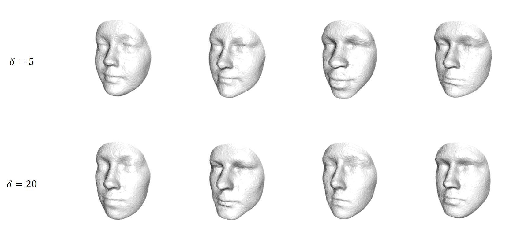
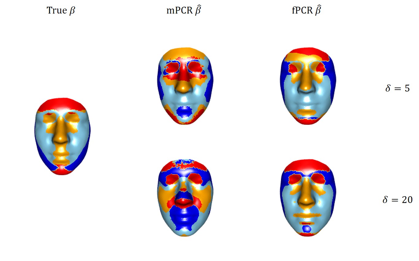
Here δ𝛿\delta is a positive constant signifying the strength of the effect, X𝒩(0,1)similar-to𝑋𝒩01X\sim\mathcal{N}(0,1), β(m)𝛽𝑚\beta(m) is a coefficient function, ϵ(m)italic-ϵ𝑚\epsilon(m) is an error function, and γnisubscript𝛾𝑛𝑖\gamma_{ni} is an iid measurement noise. To ensure a realistic simulation, we take β(m)𝛽𝑚\beta(m) to be the estimated β(m)𝛽𝑚\beta(m) for height from Section 4. A plot of this β𝛽\beta is given in the top left of Figure 2. The error, ε(m)𝜀𝑚\varepsilon(m) is constructed by randomly selecting one of the faces from the ADAPT study, while the γnisubscript𝛾𝑛𝑖\gamma_{ni} is a vector of 𝒩(0,0.002)𝒩00.002\mathcal{N}(0,0.002) displacements to each x, y, and z coordinate. The examples of simulated faces are as in Figure 1. The plots shown are based on δ=20𝛿20\delta=20.

Refer to caption
Figure 1: Examples of simulated faces for δ=5𝛿5\delta=5 (top) and δ=20𝛿20\delta=20 (bottom).

We repeated the simulation 1000 times for δ=0𝛿0\delta=0, δ=5𝛿5\delta=5, δ=20𝛿20\delta=20, δ=50𝛿50\delta=50, δ=100𝛿100\delta=100, and δ=200𝛿200\delta=200 and for each run N=100𝑁100N=100 is taken. We compared the rejection rates based on PCA test, Choi test, and norm test for multivariate PCR and functional PCR. For multivariate PCR, we ran principal component analysis on pooled data, stacking x-coordinate values, y-coordinate values, and z-coordinate values of the 7150 quasi-landmarks on the faces. We then took principal components that explain 99 % of the total variation, used them as our response, and fit a linear regression model with predictor X𝑋X. We have compared this to our method, functional PCR. It is not very conventional to conduct a PCA test, Choi test, or norm test in the multivariate case, since those tests target infinite dimensional spaces. However, to make a proper comparison, we have used the same testing methods.

The results are summarized in Table 1. It shows that the rejection rates for δ=0𝛿0\delta=0 is within 2 standard error of 0.05, the alpha level we took. As δ𝛿\delta increases, the rejection rate increases as expected, and when δ=200𝛿200\delta=200 the rejection rate becomes almost 1. In most of cases, the rejection rates for functional PCR are bigger than the rejection rates for multivariate PCR, except a few cases like Choi test for δ=20𝛿20\delta=20.

δ𝛿\delta type rej rate PCA rej rate Choi rej rate norm
0 multivartate 0.044 0.061 0.038
functional 0.059 0.064 0.060
5 multivariate 0.054 0.070 0.049
functional 0.078 0.078 0.069
20 multivariate 0.063 0.090 0.061
functional 0.097 0.101 0.094
50 multivariate 0.136 0.221 0.181
functional 0.265 0.299 0.293
100 multivariate 0.474 0.739 0.596
functional 0.662 0.768 0.745
200 multivariate 0.989 1.000 0.997
functional 0.999 1.000 0.999
Table 1: The rejection rates based on three different tests (PCA test, Choi test, and norm test) for different δ𝛿\delta’s. For δ=0𝛿0\delta=0 case, the rejection rates are approximately 0.05, the alpha in this case, and for the other cases, the rejection rates for functional PCR are higher than the rejection rates for multivariate PCR.

Some examples of estimated betas from functional PCR and from multivariate PCR are given in Figure 2. Red and yellow colors are where beta shows outward effect, meaning that in those parts the face goes outward when predictor increases, while blue and skyblue means that beta shows inward effect. Since it is height we have used, the plot in left shows that the face would become prolonged as the predictor increases. And the plots show that the estimated beta from functional PCR picks up the smoothness of the original beta and better resembles the original beta, while the estimated beta from multivariate PCR shows rough edges and sometimes gives very different effect as in the bottom (δ=20𝛿20\delta=20 case).

Refer to caption
Figure 2: Examples of estimated beta. The left is the beta used for simulation, the middle is the estimated beta from multivariate PCR, and the right is the estimated beta from functional PCR. The top row is for δ=5𝛿5\delta=5 and the bottom row is for δ=20𝛿20\delta=20. Red and yellow means that beta shows outward effect while blue and skyblue means that beta shows inward effect.

4 ADAPT Study

This section presents the application of our methodologies from Section 2 to the ADAPT data. We convert the 3D facial imaging data into functional objects in Section 4.1, where we also discuss the details on how to apply each step of the framework in Section 2.1. Section 4.2 presents the principal components of our 2-step FPCA from Section 2.2. Section 4.3 presents a regression model with the 3D faces as manifold outcomes and the covariates age, gender, height, weight, and genetic ancestry; we discuss the effects and significances of the resulting coefficient functions.

4.1 Facial Functional Object Construction

We view each face as a 2-dimensional manifold that is a subset of 3superscript3\mathbb{R}^{3}, and our goal is to construct functional objects 𝐘n:𝐌03:subscript𝐘𝑛subscript𝐌0superscript3{\bf Y}_{n}:{\bf M}_{0}\rightarrow\mathbb{R}^{3} from each face. There are 6564 faces, and each face is sampled densely with 7150 points in x, y, and z coordinates. Therefore, the data is {ynpq:n=1,,6564;p=1,,7150;q=1,2,3}conditional-setsubscripty𝑛𝑝𝑞formulae-sequence𝑛16564formulae-sequence𝑝17150𝑞123\{\mathrm{y}_{npq}:n=1,\cdots,6564;p=1,\cdots,7150;q=1,2,3\}. We elaborate each step of constructing facial functional objects as below.

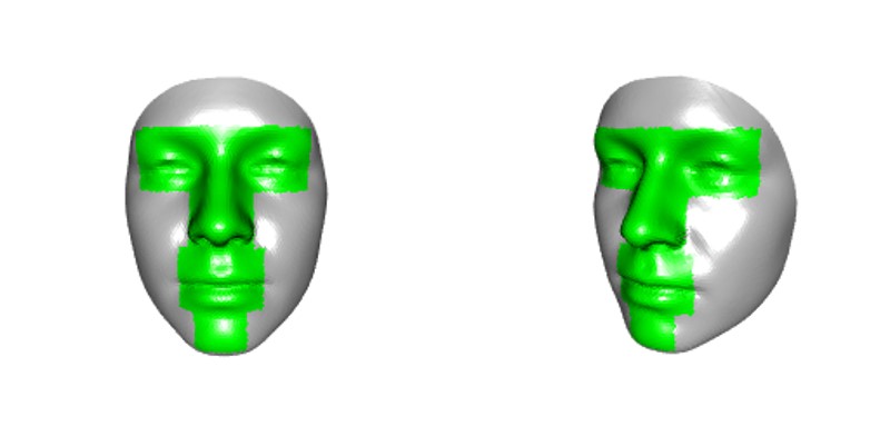
Step 1. We identified a reference face 0subscript0\mathcal{M}_{0} as the mean of the 6564 faces, that is, {y¯pq:y¯pq=1Nn=1Nynpq;p=1,,7150;q=1,2,3}conditional-setsubscript¯y𝑝𝑞formulae-sequencesubscript¯y𝑝𝑞1𝑁superscriptsubscript𝑛1𝑁subscripty𝑛𝑝𝑞formulae-sequence𝑝17150𝑞123\{\bar{\mathrm{y}}_{pq}:\bar{\mathrm{y}}_{pq}=\frac{1}{N}\sum_{n=1}^{N}\mathrm{y}_{npq};p=1,\cdots,7150;q=1,2,3\}. This approach is possible because the data were already aligned via Procrustes analysis; the resulting mean face is given in Figure 3.
Refer to caption
Figure 3: Plots of mean face which is taken as a reference face. Green area represents the area where finer mesh is taken for FELSPLINE basis functions. Examples of mesh plots are as in Figure 4.

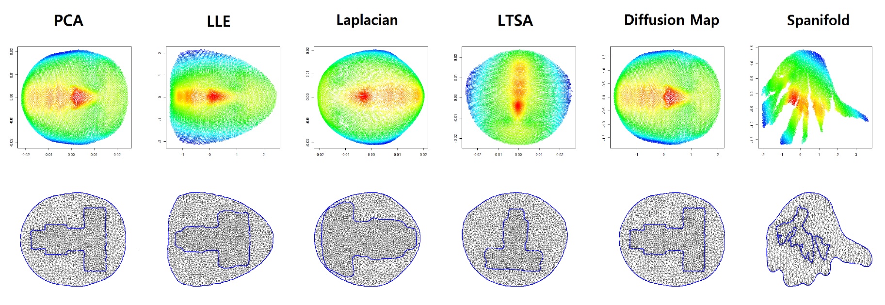
Step 2. We apply manifold learning techniques to the mean face to find 𝐌0subscript𝐌0{\bf M}_{0}, the representation of mean face in 2superscript2\mathbb{R}^{2}. The resulting 𝐌0subscript𝐌0{\bf M}_{0} is represented by {mpq;p=1,,7150,q=1,2,3}formulae-sequencesubscriptm𝑝𝑞𝑝17150𝑞123\{\mathrm{m}_{pq};p=1,\cdots,7150,q=1,2,3\}. The choice of the manifold learning technique for constructing 𝐌0subscript𝐌0{\bf M}_{0} is important to obtain a reasonable functional object that is close to the original data. Figure 4 shows how 𝐌0subscript𝐌0{\bf M}_{0} changes with different manifold learning techniques. Since smoothness is defined with distance along 0subscript0\mathcal{M}_{0}, we believed that the manifold learning techniques that preserve local distances would work best. In order to check our intuition, we tried several nonlinear dimension reduction techniques like local linear embedding (LLE, Saul and Roweis (2003)), Laplacian eigenmaps (Belkin and Niyogi, 2003), Isomap (Tenenbaum et al., 2000), local tangent space alignment (LTSA, Zhang and Zha (2004)), Diffusion Map (Nadler et al., 2006), and Spanifold Chenouri et al. (2015) along with a linear dimension reduction technique principal component analysis (PCA) for a comparison.

Step 3. We need to align all faces to the reference face, but the faces are already aligned using a generalized Procrustes superimposition (Rohlf and Slice, 1990) as discussed in Section 1.1. Therefore, we can infer that the faces are also aligned to the reference manifold 0subscript0\mathcal{M}_{0}, the mean face.

Step 4. We construct basis functions 𝐞j:[𝐌02]3:subscript𝐞𝑗delimited-[]subscript𝐌0superscript2superscript3{\bf e}_{j}:[{\bf M}_{0}\subset\mathbb{R}^{2}]\rightarrow\mathbb{R}^{3}, but given the limitations in constructing such basis functions, we took basis functions ej:[𝐌02]:subscript𝑒𝑗delimited-[]subscript𝐌0superscript2e_{j}:[{\bf M}_{0}\subset\mathbb{R}^{2}]\rightarrow\mathbb{R} to expand the functional objects marginally

𝐘n(m)=[Yn1Yn2Yn3](m)=j=1J[bnj1bnj2bnj3]ej(m)subscript𝐘𝑛𝑚matrixsubscript𝑌𝑛1subscript𝑌𝑛2subscript𝑌𝑛3𝑚superscriptsubscript𝑗1𝐽matrixsubscript𝑏𝑛𝑗1subscript𝑏𝑛𝑗2subscript𝑏𝑛𝑗3subscript𝑒𝑗𝑚{\bf Y}_{n}(m)=\begin{bmatrix}Y_{n1}\\ Y_{n2}\\ Y_{n3}\end{bmatrix}(m)=\sum_{j=1}^{J}\begin{bmatrix}b_{nj1}\\ b_{nj2}\\ b_{nj3}\end{bmatrix}e_{j}(m) (12)

where Yn1subscript𝑌𝑛1Y_{n1} corresponds to x coordinate of 𝐘nsubscript𝐘𝑛{\bf Y}_{n}, Yn2subscript𝑌𝑛2Y_{n2} corresponds to y coordinate of 𝐘nsubscript𝐘𝑛{\bf Y}_{n}, and Yn3subscript𝑌𝑛3Y_{n3} corresponds to z coordinate of 𝐘nsubscript𝐘𝑛{\bf Y}_{n}. We find {b^njq}subscript^𝑏𝑛𝑗𝑞\{\hat{b}_{njq}\} for q=1,2,3𝑞123q=1,2,3 by minimizing equation 1. We used FELSPLINEs (Ramsay, 2002) which are designed for irregularly shaped domain with complex boundaries and use a finite element method, meaning that the domain is divided into triangular meshes and piecewise linear and quadratic functions are fit on each mesh. Therefore, we needed to create meshes out of our domain. Ramsay (2002) uses all data points as vertices of the mesh, but in our case that will return over twenty thousand basis functions. In order to limit the number of basis functions to less than the number of observations per face, which is 7150 in our data, we created new meshes using the R package INLA (Lindgren and Rue, 2013).

There can be many different ways to create meshes, and the choice of mesh is closely related to the number of basis functions, thus affecting how close the functional objects are to the data. We took a finer mesh around periorbital, perinasal, and perioral areas shown as the green area in Figure 3, as these localized facial features are emphasized in (Hammond et al., 2005), and a coarser mesh around the cheeks and forehead where the surface is more smooth. The meshes for different manifold learning techniques are given in the bottom row of plots of Figure 4.
Refer to caption
Figure 4: The dimension-reduced reference manifold 𝐌0subscript𝐌0{\bf M}_{0} and corresponding mesh using different manifold learning techniques. The finer inner mesh correspond to the area of green in Figure 3.

Table 2 presents the average mean squared errors (AMSE) of 100 randomly selected faces, which is a measure of how close the functional objects 𝐘n(m)subscript𝐘𝑛𝑚{\bf Y}_{n}(m) are to the original data {ynpq}subscripty𝑛𝑝𝑞\{\mathrm{y}_{npq}\}:

AMSE:1N1Pn=1Np=1P|ynp𝐘n(mp)|2,AMSE:1𝑁1𝑃superscriptsubscript𝑛1𝑁superscriptsubscript𝑝1𝑃superscriptsubscripty𝑛𝑝subscript𝐘𝑛subscript𝑚𝑝2\text{AMSE:}\quad\quad\frac{1}{N}\frac{1}{P}\sum_{n=1}^{N}\sum_{p=1}^{P}|{\bf\mathrm{y}}_{np}-{\bf Y}_{n}(m_{p})|^{2}, (13)

where N=100𝑁100N=100 and P=7150𝑃7150P=7150. We stress that, at this stage, we are not aiming for dimension reduction; our goal is to approximate the data using basis functions with as little error as possible. Therefore, in this step we want the AMSE to be as small as possible to minimize any information loss when converting to functional objects. However, the Procustes Analysis used to initially align and scale the data results in a unit-less scale for the coordinates of the face; the x-axis has been rescaled to have a range of 1. This means that the AMSE values themselves are difficult to interpret, and thus we focus on comparisons of the AMSE’s. The range of the first coordinate of the domain points 𝐦nsubscript𝐦𝑛{\bf m}_{n}, {mp1}subscriptm𝑝1\{\mathrm{m}_{p1}\}, is different for each 𝐌0subscript𝐌0{\bf M}_{0} from the different manifold learning techniques, and thus we made the smoothing parameter, λ𝜆\lambda, in equation 1 dependent on the range of x. The AMSE for LTSA with λ3subscript𝜆3\lambda_{3} is smallest, while the AMSE for LLE with λ1subscript𝜆1\lambda_{1} is also similarly small. Both LTSA and LLE try to preserve neighborhood distances of the original manifold, which confirms our intuition that they would best represent smoothness defined with distances along 𝐌0subscript𝐌0{\bf M}_{0} and thus give a good fit. Spanifold gives the largest AMSE, which is not surprising given that the 𝐌0subscript𝐌0{\bf M}_{0} is very irregular. This is because a human face face has many local peaks, and Spanifold works better with more regular surfaces.

PCA LLE Laplacian LTSA Diffusion Map Spanifold
λ1subscript𝜆1\lambda_{1} 0.00247 0.00018 0.00423 0.00078 0.00056 0.00679
λ2subscript𝜆2\lambda_{2} 0.00084 0.00036 0.00167 0.00017 0.00078 0.00690
λ3subscript𝜆3\lambda_{3} 0.00058 0.00083 0.00114 0.00013 0.00142 0.00772
range(x) 0.046 3.900 0.041 0.051 3.906 5.671
Table 2: The pointwise mean squared errors of 𝐘(m)𝐘𝑚{\bf Y}(m) of 100 randomly selected faces as in equation 13 for different λ𝜆\lambda’s from mesh as in Figure 4. λ1subscript𝜆1\lambda_{1} = range(x)/104superscript10410^{4}, λ2subscript𝜆2\lambda_{2} = range(x)/105superscript10510^{5}, λ3subscript𝜆3\lambda_{3} = range(x)/106superscript10610^{6} where range(x) is the range of {mp1}subscriptm𝑝1\{\mathrm{m}_{p1}\}.

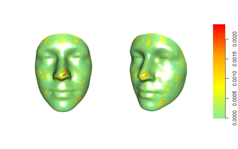
For all subsequent analyses, we utilize the manifold objects constructed using the presented LTSA mesh and used λ𝜆\lambda a little less than λ3subscript𝜆3\lambda_{3} to recover the details of face. Figure 6 shows that the facial functional objects are very close to the original faces except for some smoothing. Figure 5 shows a heatmap of the pointwise errors between functional objects and the original data. The tip of the nose shows a relatively high pointwise error compared to the other areas, which is due to smoothing. The boundary does not show much deviation and seems to be stable. We believe the resulting objects are reasonable approximations of the original faces.
Refer to caption
Figure 5: Plot shows pointwise mean squared errors across all 6564 faces. This shows that the difference between the original faces and facial functional objects are very small.
Refer to caption
Figure 6: Top three plots are examples of facial data of ADAPT, {ynpq}subscripty𝑛𝑝𝑞\{\mathrm{y}_{npq}\}, and bottom three plots are corresponding facial functional objects, 𝐘n(m)subscript𝐘𝑛𝑚{\bf Y}_{n}(m). This shows that the facial functional objects closely resembles the original faces.

4.2 Functional Principal Component Analysis

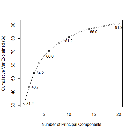
In this section we apply the 2-step Functional Principal Component Analysis (2-step FPCA) discussed in Section 2.2 to the ADAPT data. We take H=200𝐻200H=200 principal components, or ψh(m)subscript𝜓𝑚\psi_{h}(m), in the first step (pooling coordinates), which accounts for 99.9% of the total variance. In the second step we then compute the PCs without pooling coordinates,𝐕k(m)subscript𝐕𝑘𝑚{\bf V}_{k}(m), and Figure 7 shows the cumulative proportion of explained variance. The first principal component 𝐕1(m)subscript𝐕1𝑚{\bf V}_{1}(m) explains 31.27%, the second principal component 𝐕2(m)subscript𝐕2𝑚{\bf V}_{2}(m) explains 12.43%, and the third principal component 𝐕3(m)subscript𝐕3𝑚{\bf V}_{3}(m) explains 10.59% of variation. The first 5 principal components combined explain 66.71%, and the first 10 principal components combined explain 81.26%.
Refer to caption
Figure 7: Cumulative proportion of variance for number of PCs. First 10 PCs explain about 81.2% of total variance and first 18 PCs explain about 90.2% of total variance.

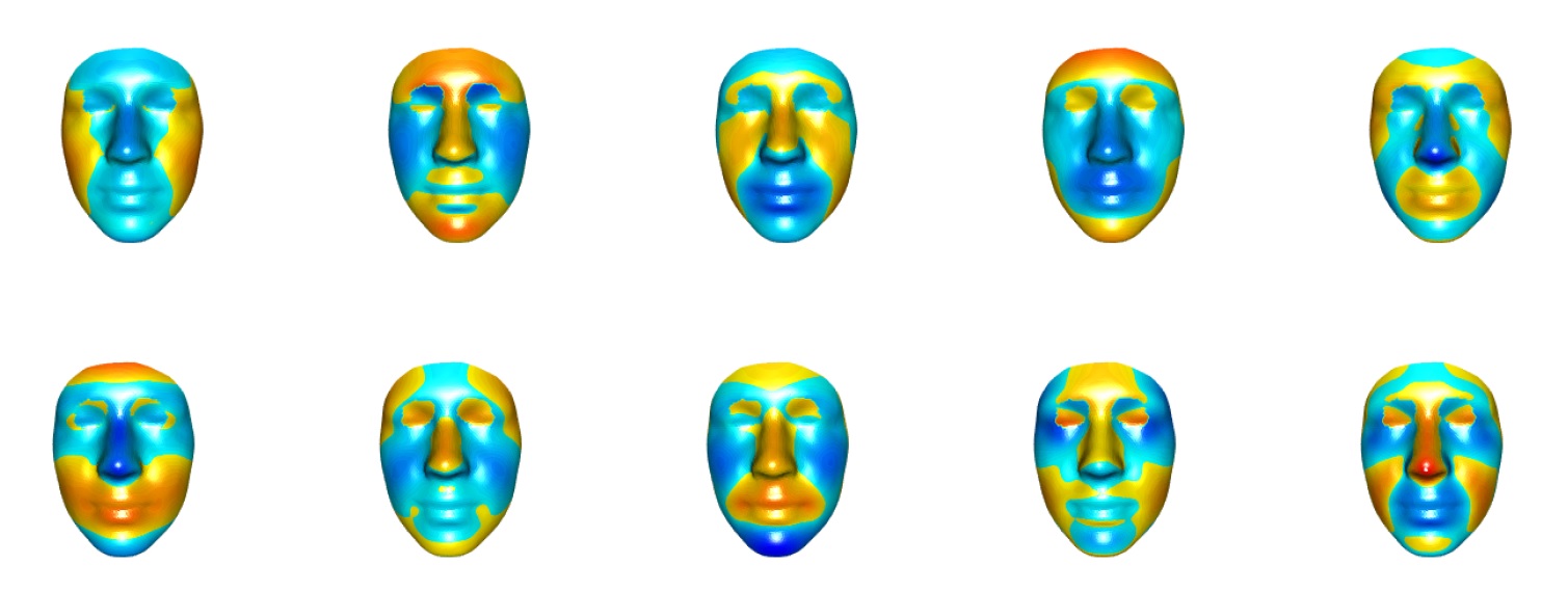
In Figure 8, we demonstrate how each principal component affects the face, which, given that we are working in 3D is a bit challenging to visualize. We thus compute the orthogonal vector, 𝐭psubscript𝐭𝑝{\bf t}_{p}, to the tangent plane of each facial point, mpsubscriptm𝑝{\bf\mathrm{m}}_{p}, by conducting traditional PCA in a small neighborhood of mpsubscript𝑚𝑝m_{p} (distance 0.1). As the first and second principal components would be the two vectors spanning the tangent plane, the third principal component would be the vector orthogonal to the tangent plane. Note that PCA also gives |𝐭p|2=1superscriptsubscript𝐭𝑝21|{\bf t}_{p}|^{2}=1. We then calculated the inner product 𝐕k(mp),𝐭psubscript𝐕𝑘subscript𝑚𝑝subscript𝐭𝑝\langle{\bf V}_{k}(m_{p}),{\bf t}_{p}\rangle at each point for p=1,,7150𝑝17150p=1,\cdots,7150. The yellow to red area in Figure 8 denotes a PC whose effect points outward while the lightblue to blue area means that the effect of PC at that point is inward. Orange and lightblue mean weaker effects and red and blue mean stronger effects.
Refer to caption
Figure 8: The directional plots for PC 1-5 on the top and PC 6-10 on the bottom. The color on the face shows the direction and the strength, from weakest to strongest, of each PC effect on face: from lightblue to blue, inward, and from yellow to red, outward.

As the top leftmost plot of Figure 8 suggests, the major difference between the mean face and the reconstructed faces using the first PC in Figure 9 is the sides of the faces. The top face became thinner while the middle face became a little rounder on the cheek. Figure 9 shows the progression of facial changes with more PCs included. The rightmost faces are good approximations to the bottom plots in Figure 6, explaining 91.39% of total variation. Thus we have now reduced the dimension of the data from 7150 points to 20 principal components, while carefully controlling the information loss.
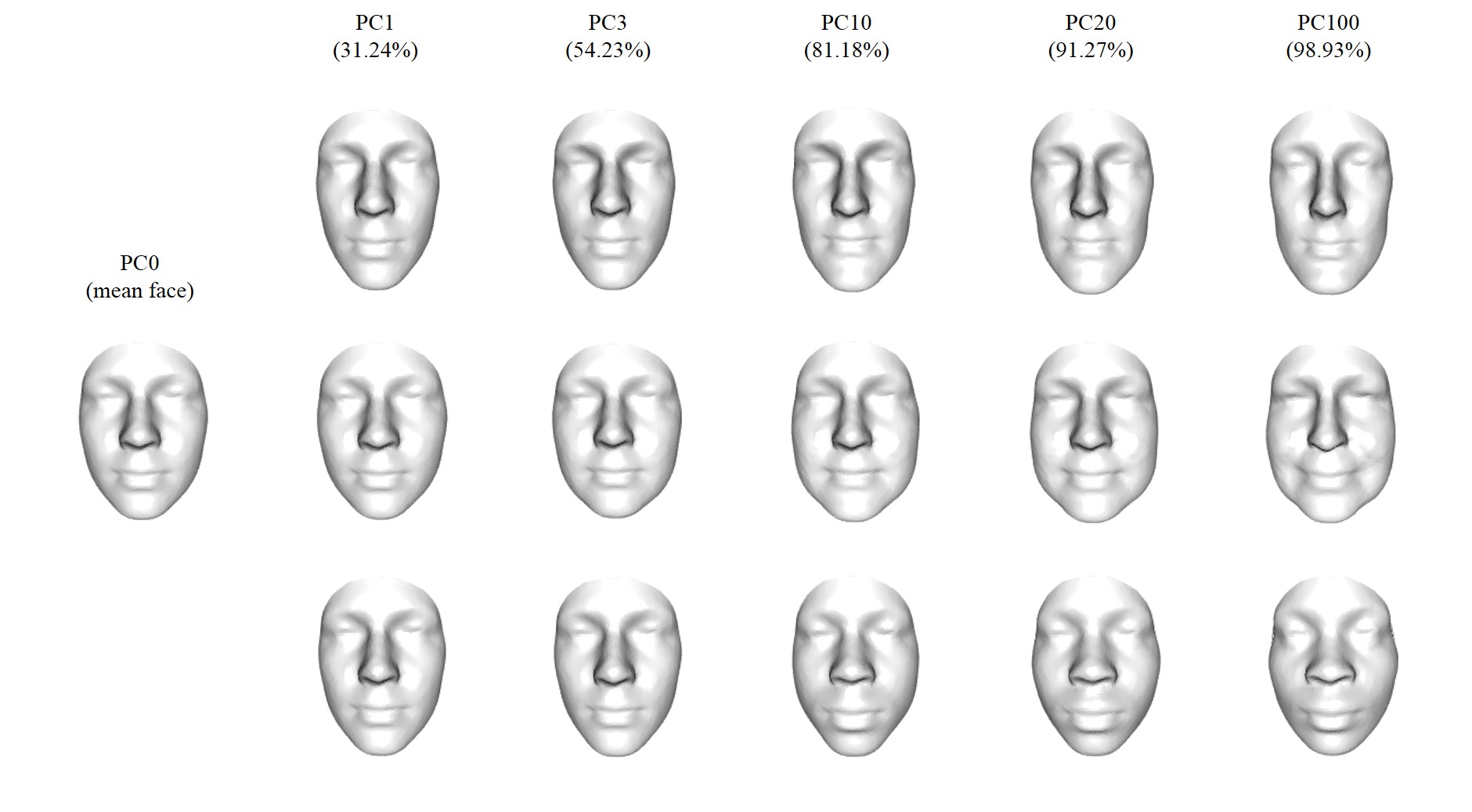
Refer to caption
Figure 9: Three facial functional objects expanded using different number of PCs from the second step of FPCA. Leftmost plot is the mean face. The percentage of variation explained is given at the top of each column.

4.3 Manifold-on-Scalar Regression

We conclude the application section by carrying out Manifold-on-Scalar Regression, which represents a major strength of our methodology. We examine the effects of sex, age, height, weight, and genetic ancestry the structure of human faces. Genetic ancestry is measured as a proportion of a particular ethnic background, where E.ASN refers to East Asian, S.ASN refers to South Asian, AMR refers to Native American, W.AFR refers to West African, and S.EUR refers Southern European. There is also N.EUR which refers to Northern European, but since the sum of all proportions is 1, it is removed from the covariates, meaning that it is acting as the ancestral baseline, so all ancestral effects indicate differences from Northern Europeans. For the response variable, we take the facial functional objects 𝐘n(m)subscript𝐘𝑛𝑚{\bf Y}_{n}(m) expanded with K=100𝐾100K=100 principal components from the FPCA in Section 4.2. The model is as in (14). Since the genetic ancestry was not computed for all individuals, the number of facial manifolds involved in the model is N=3287𝑁3287N=3287. The model also includes a 𝒩(0,10)𝒩010\mathcal{N}(0,10) noise variable just as a check to make sure our subsequent p-values have proper specificity.

𝐘n(m)=β0(m)+β1(m)sexn+β2(m)agen+β3(m)heightn+β4(m)weightn+β5(m)pnE.ASN+β6(m)pnS.ASN+β7(m)pnAMR+β8(m)pnW.AFR+β9(m)pnS.EUR+β10(m)(sexn×agen)+β11(m)(agen×weightn)+β12(m)(heightn×weightn)+β13(m)noisen+ϵn(m).subscript𝐘𝑛𝑚subscript𝛽0𝑚subscript𝛽1𝑚subscriptsex𝑛subscript𝛽2𝑚subscriptage𝑛subscript𝛽3𝑚subscriptheight𝑛subscript𝛽4𝑚subscriptweight𝑛subscript𝛽5𝑚subscriptsuperscript𝑝E.ASN𝑛subscript𝛽6𝑚subscriptsuperscript𝑝S.ASN𝑛subscript𝛽7𝑚subscriptsuperscript𝑝AMR𝑛subscript𝛽8𝑚subscriptsuperscript𝑝W.AFR𝑛subscript𝛽9𝑚subscriptsuperscript𝑝S.EUR𝑛subscript𝛽10𝑚subscriptsex𝑛subscriptage𝑛subscript𝛽11𝑚subscriptage𝑛subscriptweight𝑛subscript𝛽12𝑚subscriptheight𝑛subscriptweight𝑛subscript𝛽13𝑚subscriptnoise𝑛subscriptitalic-ϵ𝑛𝑚\begin{split}{\bf Y}_{n}(m)&={\bf\beta}_{0}(m)+{\bf\beta}_{1}(m)\text{sex}_{n}+{\bf\beta}_{2}(m)\text{age}_{n}+{\bf\beta}_{3}(m)\text{height}_{n}+{\bf\beta}_{4}(m)\text{weight}_{n}\\ &+{\bf\beta}_{5}(m)p^{\text{E.ASN}}_{n}+{\bf\beta}_{6}(m)p^{\text{S.ASN}}_{n}+{\bf\beta}_{7}(m)p^{\text{AMR}}_{n}+{\bf\beta}_{8}(m)p^{\text{W.AFR}}_{n}+{\bf\beta}_{9}(m)p^{\text{S.EUR}}_{n}\\ &+{\bf\beta}_{10}(m)(\text{sex}_{n}\times\text{age}_{n})+{\bf\beta}_{11}(m)(\text{age}_{n}\times\text{weight}_{n})\\ &+{\bf\beta}_{12}(m)(\text{height}_{n}\times\text{weight}_{n})+{\bf\beta}_{13}(m)\text{noise}_{n}+{\bf\epsilon}_{n}(m).\end{split} (14)

We estimated beta functions βrsubscript𝛽𝑟\beta_{r}’s with regularization term as outlined in Section 2.3. The tuning parameter λrsubscript𝜆𝑟\lambda_{r}’s are determined using iterative 4-fold cross validation.

The sizes and p-values of resulting β^rsubscript^𝛽𝑟\hat{\beta}_{r} are presented in Table 3. We utilize three different tests as outlined in Choi and Reimherr (2016). Each test uses slightly different normalizations of the estimated parameter functions. The first test is based on the L2superscript𝐿2L^{2}-norm, which ignores the covariance operator of the parameter estimate (though it is used in calculating p-values). The other two approaches attempt to normalize by the covariance operator, where the PC and Choi approach normalize by the Moore-Penrose inverse of the covariance operator and square-root of the covariance operator, respectively. Both approaches can be phrased using PCA, and we refer the interested reader to Choi and Reimherr (2016) for more details.

The asymptotic distribution of the PC approach is simply a chi-squared distribution, while the norm and Choi approach are given by weighted sums of chi-squares. We approximate p-values from the weighted distribution using Imhof’s method (Imhof, 1961; Duchesne and Lafaye de Micheaux, 2010). The p-values suggest that all beta functions are significant at 99% significance level except the noise. Therefore, the tests seem to have discerned the effects from the true negative variable.

Predictor β^r2superscriptnormsubscript^𝛽𝑟2\|\hat{\beta}_{r}\|^{2} p-value (PC) p-value (Choi) p-value (Norm)
β0subscript𝛽0\beta_{0} 3.910e-05 << 1.110e-21 5.385e-15 2.631e-09
β1subscript𝛽1\beta_{1} sex 9.924e-07 << 1.110e-21 5.551e-16 1.443e-15
β2subscript𝛽2\beta_{2} age 4.443e-10 5.888e-11 3.053e-15 3.672e-04
β3subscript𝛽3\beta_{3} height 2.105e-09 << 1.110e-21 5.551e-17 3.514e-14
β4subscript𝛽4\beta_{4} weight 1.549e-09 9.826e-08 6.088e-06 1.173e-02
β5subscript𝛽5\beta_{5} pE.ASNsuperscript𝑝E.ASNp^{\text{E.ASN}} 2.439e-06 << 1.110e-21 4.996e-15 3.164e-15
β6subscript𝛽6\beta_{6} pS.ASNsuperscript𝑝S.ASNp^{\text{S.ASN}} 5.859e-07 1.332e-17 2.220e-16 1.720e-11
β7subscript𝛽7\beta_{7} pAMRsuperscript𝑝AMRp^{\text{AMR}} 7.689e-07 1.418e-21 1.110e-16 1.357e-08
β8subscript𝛽8\beta_{8} pW.AFRsuperscript𝑝W.AFRp^{\text{W.AFR}} 1.783e-06 << 1.110e-21 1.110e-15 7.772e-16
β9subscript𝛽9\beta_{9} pS.EURsuperscript𝑝S.EURp^{\text{S.EUR}} 1.514e-06 << 1.110e-21 6.661e-16 8.826e-14
β10subscript𝛽10\beta_{10} sex ×\times age 2.103e-10 1.988e-19 5.551e-17 2.034e-10
β11subscript𝛽11\beta_{11} age ×\times weight 3.523e-14 7.790e-06 5.328e-11 9.143e-03
β12subscript𝛽12\beta_{12} height ×\times weight 7.553e-14 3.521e-10 5.074e-07 1.488e-03
β13subscript𝛽13\beta_{13} noise 4.188e-12 3.419e-01 3.242e-01 5.647e-01
Table 3: The size of β^rsubscript^𝛽𝑟\hat{\beta}_{r} and p-values based on PC test, Choi test, and Norm test are presented.

Now that we have carried out our hypothesis testing, it is important to visualize and more fully understand the estimated beta functions. Since these functions have domain of 𝐌0subscript𝐌0{\bf M}_{0}, plotting βrsubscript𝛽𝑟\beta_{r} is challenging. Instead, we visualize the effects in a manner similar to the PC functions in Section 4.2; at each point we examine how strong the effect is in the orthogonal direction to the tangent plane (i.e. outward or inward relative to the face).

We provide three different plot types: directional plots, pointwise significance plots, and overall significance plots that control the Type 1 error rate simultaneously across the face. The directional plot shows how the beta function affects the face, the pointwise significance plot shows the facial areas where each point is tested positive (blue/red means positive at 99% level and lightblue/orange means positive at 95% level), and the overall significance plot shows the facial areas that have overall significance at 99% level. An advantage of applying functional data analysis tools to faces are these overall significance plots, which rely heavily on the functional nature of the data.

We discuss only a few of the estimated effects here to highlight how to interpret our results. Further discussion can be found in the supplemental. For example, the middle plot of Figure 10 presents the effect for sex, demonstrating the difference between the average male and female face, for a subject that is 30 years old, 170cm tall, and weighs 70kg. Blue denotes an inward effect, while red represents an outward effect. The female face is rounder than the male’s as signified by the red parts around the cheek in the directional plot. It also shows that the male has a more pronounced nose, and the female has a rounder eye area with red on the eyelids and blue on the eyebrow area. Those areas are shown as significant for both pointwise significance plot and overall significance plot.

Refer to caption
Figure 10: The left two plots are predicted faces of 30-year-old, 170cm-tall, 70kg-heavy Northern European male and female. The right three plots show the effect of beta of sex.

The effect of the proportion of East Asian descent is shown in Figure 11. As Northern European proportion is taken as the base, the beta function indicates the difference between Northern European and East Asian. We see that the average East Asian face is rounder, has a lower nose, and a less pronounced eyebrow. The overall significance plot (right most plot) shows that the nose, cheek, and forehead area are still statistically significant at a 99% significance level when correcting for multiple testing across the entire face using our confidence bubbles.

Refer to caption
Figure 11: The left two plots are predicted faces of 25-year-old, 165cm-tall, 65kg-heavy Northern European and East Asian female. The right three plots show the effect of the corresponding beta.

The effect of the proportion of Western African is shown in Figure 12. The most features seem to be the nose and mouth, and those are picked up in the overall significance plot. The nose of Western African is more flattened but more wider than that of Northern European, shown as the inward effect (blue) in the middle of nose, and the outward effect (red) on the sides of nose. The lips are more outward, and the lower cheek area difference is also picked up in the overall significance plot.

Refer to caption
Figure 12: The left two plots are predicted faces of 25-year-old, 165cm-tall, 65kg-heavy Northern European and Western African female. The right three plots show the effect of beta of the corresponding beta.

5 Discussion

We have presented a new framework that facilitates the analysis of 3D imaging data sampled at a high-resolution. We view Manifold Data Analysis (MDA) as a subbranch of Functional Data Analysis (FDA), which incorporates ideas and techniques from shape analysis and manifold learning. MDA allows a wide variety of functional data analysis tools to be applied to data that includes a manifold variable by converting each manifold unit into a functional object. Through this method, the dimension of the data is reduced and smoothness of data can be exploited. Extensions of functional data techniques are introduced to the manifold setting: 2-step functional principal component analysis and manifold-on-scalar regression. Our methods are illustrated using 3D facial images.

This paper opens up a broad range of future work. In constructing functional objects, there are many choices to be made including the manifold learning technique for domain construction, the basis system for functional unit construction, and the tuning parameter selection. Here we used the FELSPLINE basis which also leads to further issues of how to construct the domain mesh. Alternative basis functions could prove useful, especially kernel methods that allow for irregular multidimensional domains as well as multivariate functions. Also, other extensions of functional data techniques for manifold data can be developed.

Lastly, we believe that these techniques will prove useful to a variety of applications. As part of the big data revolution occurring in the sciences, many types of high-frequency or high-resolution data are being collected. Data which include samples of manifolds will become increasingly common, especially in biomedical imaging. FDA tools naturally exploit smoothness and we thus believe the will be useful for analyzing data involving manifolds. As computational tools progress, we will be likely able to work with deformation maps that directly map one manifold to another, even if those manifolds reside in 3D space. However, the computational challenges may be substantial, especially if more complicated statistical models are to be employed. For example, building nonlinear or varying coefficient models where the outcome is a manifold. Or, as we aim to do in a future work, if one wants to carry out a regression with a large number predictors (e.g. genetic markers). There are many open practical and methodological issues that remain to be explored.

References

  • Ahonen et al. [2006] T. Ahonen, A. Hadid, and M. Pietikainen. Face description with local binary patterns: Application to face recognition. IEEE transactions on pattern analysis and machine intelligence, 28(12):2037–2041, 2006.
  • Belkin and Niyogi [2003] M. Belkin and P. Niyogi. Laplacian eigenmaps for dimensionality reduction and data representation. Neural Computation, 15:1373–1396, 2003.
  • Chen and Müller [2012] D. Chen and H. Müller. Nonlinear manifold representations for functional data. The Annals of Statistics, 40:1–29, 2012.
  • Chenouri et al. [2015] S. E. Chenouri, P. Kobelevskiy, and C. G. Small. Spanifold: spanning tree flattening onto lower dimension. Stat, 4:15–31, 2015.
  • Choi and Reimherr [2016] H. Choi and M. Reimherr. A geometric approach to confidence regions and bands for functional parameters. 2016.
  • Claes et al. [2012] P. Claes, W. Walters, and J. Clement. Improved facial outcome assessment using a 3d anthropometric mask. International Journal of Oral and Maxillofacial Surgery, 41(3):324–330, 2012.
  • Claes et al. [2014a] P. Claes, H. Hill, and M. D. Shriver. Toward dna-based facial composites: preliminary results and validation. Forensic Sci Int Genet, 13:208–16, 2014a.
  • Claes et al. [2014b] P. Claes, D. K. Liberton, K. Daniels, K. M. Rosana, E. E. Quillen, L. N. Pearson, B. McEvoy, M. Bauchet, A. A. Zaidi, W. Yao, H. Tang, G. S. Barsh, D. M. Absher, …, and M. D. Shriver. Modeling 3d facial shape from dna. PLoS Genet, 10(3), 2014b.
  • Dimeglio et al. [2014] C. Dimeglio, S. Gallón, J. Loubes, and E. Maza. A robust algorithm for template curve estimation based on manifold embedding. Computational Statistics and Data Analysis, 70:373–386, 2014.
  • Drira et al. [2012] H. Drira, B. B. Amor, M. Daoudi, A. Srivastava, and S. Berretti. 3d dynamic expression recognition based on a novel deformation vector field and random forest. ICPR, pages 1104––1107, 2012.
  • Duchesne and Lafaye de Micheaux [2010] P. Duchesne and P. Lafaye de Micheaux. Computing the distribution of quadratic forms: Further comparisons between the liu-tang-zhang approximation and exact methods. Computational Statistics and Data Analysis, 54:858–862, 2010.
  • Elhamifar and Vidal [2011] E. Elhamifar and R. Vidal. Sparse manifold clustering and embedding. In Advances in neural information processing systems, pages 55–63. NIPS Foundation, 2011.
  • Ellingson et al. [2013] L. Ellingson, V. Patrangenaru, and F. Ruymgaart. Nonparametric estimation of means on Hilbert manifolds and extrinsic analysis of mean shapes of contours. Journal of Multivariate Analysis, 122:317–333, 2013.
  • Ettinger et al. [2016] B. Ettinger, S. Perotto, and L. M. Sangalli. Spatial regression models over two-dimensional manifolds. Biometrika, 103(1):71–88, 2016.
  • Graves et al. [2009] S. Graves, G. Hooker, and J. Ramsay. Functional Data Analysis with R and MATLAB. Springer, 2009.
  • Hammond et al. [2005] P. Hammond, T. J. Hutton, J. E. Allanson, B. Buxton, L. E. Campbell, J. Clayton-Smith, D. Donnai, A. Karmiloff-Smith, K. Metcalfe, K. C. Murphy, M. Patton, P. Barbara, K. Prescott, P. Scambler, A. Shaw, A. C. M. Smith, A. F. Stevens, I. K. Temple, R. Hennekam, and M. Tassabehji. Discriminating power of localized three-dimensional facial morphology. The American Journal of Human Genetics, 77(6):999–1010, 2005.
  • Horváth and Kokoszka [2012] L. Horváth and P. Kokoszka. Inference for Functional Data with Applications. Springer, New York, 2012.
  • Huang et al. [2014a] D. Huang, H. Ding, C. Wang, Y. Wang, G. Zhang, and L. Chen. Local circular patterns for multi-modal facial gender and ethnicity classification. Image and Vision Computing, 32:12:1181–1193, 2014a.
  • Huang et al. [2014b] D. Huang, J. Sun, X. Yang, D. Weng, and Y. Wang. A functional approach to decnonvolve dynamic neuroimaging data. Chinese Conference on Biometric Recognition, pages 1–21, 2014b.
  • Imhof [1961] J. P. Imhof. Computing the distribution of quadratic forms in normal variables. Biometrika, 48:419–426, 1961.
  • Jain and Li [2011] A. Jain and S. Li. Handbook of face recognition. New York: springer, 2011.
  • Kokoszka and Reimherr [2017] P. Kokoszka and M. Reimherr. Introduction to Functional Data Analysis. Chapman and Hall/CRC, 2017.
  • Kurtek and Drira [2015] S. Kurtek and H. Drira. A comprehensive statistical framework for elastic shape analysis of 3d faces. Computers and Graphics, 51:52–59, 2015.
  • Lee [2003] J. Lee. Introduction to Smooth Manifold. Springer New York, 2003.
  • Lila et al. [2016] E. Lila, J. A. D. Aston, and L. M. Sangalli. Smooth principal component analysis over two-dimensional manifolds with an application to neuroimaging. The Annals of Applied Statistics, 10(4):1854–1879, 2016.
  • Lindgren and Rue [2013] F. Lindgren and H. Rue. Bayesian spatial and spatiotemporal modeling with r-inla. Journal of Statistical Software, 63, 2013.
  • Mardia et al. [1979] K. Mardia, J. Kent, and J. Bibby. Multivariate analysis. Academic press, 1979.
  • Nadler et al. [2006] B. Nadler, S. Lafon, R. R. Coifman, , and I. G. Kevrekidis. Diffusion maps, spectral clustering and reaction coordinates of dynamical systems. Applied and Computational Harmonic Analysis, 21:113–127, 2006.
  • Porro-Muñoz et al. [2014] D. Porro-Muñoz, F. J. Silva-Mata, A. Revilla-Eng, I. Talavera-Bustamante, and S. Berretti. 3d face recognition by functional data analysis. Iberoamerican Congress on Pattern Recognition, pages 818–826, 2014.
  • Ramsay and Silverman [2005] J. Ramsay and B. Silverman. Functional Data Analysis. Springer, 2005.
  • Ramsay [2002] T. Ramsay. Spline smoothing over difficult regions. Journal of the Royal Statistical Society: Series B (Statistical Methodology), 64:307–319, 2002.
  • Rohlf and Slice [1990] F. J. Rohlf and D. Slice. Extensions of the procrustes method for the optimal superimposition of landmarks. Systematic Biology, 39(1), 1990.
  • Saul and Roweis [2003] L. K. Saul and S. T. Roweis. Think globally, fit locally: Unsupervised learning of low dimensional manifolds. Journal of Machine Learning Research, 4:119–155, 2003.
  • Taigman et al. [2014] Y. Taigman, M. Yang, M. Ranzato, and L. Wolf. Deepface: Closing the gap to human-level performance in face verification. Proceedings of the IEEE Conference on Computer Vision and Pattern Recognition, pages 1701–1708, 2014.
  • Tenenbaum et al. [2000] J. Tenenbaum, V. de Silva, and J. C. Langford. A global geometric framework for nonlinear dimensionality reduction. Science, 290:2319–2323, 2000.
  • Turk and Pentland [1991] M. A. Turk and A. P. Pentland. Face recognition using eigenfaces. Computer Vision and Pattern Recognition, 1991.
  • Xia et al. [2013] B. Xia, B. B. Amor, M. Daoudi, and L.Ballihi. Gender and 3d facial symmetry: What’s the relationship? Automatic Face and Gesture Recognition (FG), 2013 10th IEEE International Conference and Workshops on, 2013.
  • Xia et al. [2014] B. Xia, B. B. Amor, M. Daoudi, and H. Drira. Can 3d shape of the face reveal your age? Computer Vision Theory and Applications (VISAPP), 2014 International Conference, 2:5–13, 2014.
  • Zhang and Wang [2016] X. Zhang and J. Wang. From sparse to dense functional data and beyond. The Annals of Statistics, 44(5):2281–2321, 2016.
  • Zhang and Zha [2004] Z. Zhang and H. Zha. Principal manifolds and nonlinear dimension reduction via tangent space alignment. SIAM Journal of Scientific Computing, 26:313–338, 2004.

Online Supplemental Material

Appendix A 2-Step Functional Principal Component Analysis

Step 1.

Without loss of generality, assume that the 𝐘n(m)subscript𝐘𝑛𝑚{\bf Y}_{n}(m) have been centered and thus have mean zero. Each of the functions is expressed as

𝐘n(m)=[Yn1(m),,YnD(m)][j=1Jb^nj1ej(m),,j=1Jb^njDej(m)],subscript𝐘𝑛𝑚superscriptsubscript𝑌𝑛1𝑚subscript𝑌𝑛𝐷𝑚topsuperscriptsuperscriptsubscript𝑗1𝐽subscript^𝑏𝑛𝑗1subscript𝑒𝑗𝑚superscriptsubscript𝑗1𝐽subscript^𝑏𝑛𝑗𝐷subscript𝑒𝑗𝑚top{\bf Y}_{n}(m)=\left[Y_{n1}(m),\cdots,Y_{nD}(m)\right]^{\top}\approx\left[\sum_{j=1}^{J}\hat{b}_{nj1}e_{j}(m),\cdots,\sum_{j=1}^{J}\hat{b}_{njD}e_{j}(m)\right]^{\top},

for n=1,,N𝑛1𝑁n=1,\dots,N. We stack all of the coordinate-wise functions into a single vector of functions with dimension ND𝑁𝐷ND. We denote the resulting functions as Yl(m)subscript𝑌𝑙𝑚Y_{l}(m) where Yl(m)=Ynq(m)subscript𝑌𝑙𝑚subscript𝑌𝑛𝑞𝑚Y_{l}(m)=Y_{nq}(m) for l=N(q1)+n𝑙𝑁𝑞1𝑛l=N(q-1)+n and n=1,,N𝑛1𝑁n=1,\cdots,N, q=1,,D𝑞1𝐷q=1,\cdots,D.

We aim to find the pairs of eigenvalues ηhsubscript𝜂\eta_{h} and principal component functions ψh:𝐌0D:subscript𝜓subscript𝐌0superscript𝐷\psi_{h}:{\bf M}_{0}\to{\mathbb{R}}^{D}, for h=1,,H1𝐻h=1,\dots,H, which satisfy

ηhψh(m)=Φ(m,m)ψh(m)𝑑msubscript𝜂subscript𝜓𝑚Φ𝑚superscript𝑚subscript𝜓superscript𝑚differential-dsuperscript𝑚\eta_{h}\psi_{h}(m)=\int\Phi(m,m^{\prime})\psi_{h}(m^{\prime})dm^{\prime}

where

𝚽(m,m)=E[Yl(m)Yl(m)]𝚽𝑚superscript𝑚𝐸delimited-[]subscript𝑌𝑙𝑚subscript𝑌𝑙superscriptsuperscript𝑚top\displaystyle\mbox{\boldmath${\Phi}$}(m,m^{\prime})=E[Y_{l}(m)Y_{l}(m^{\prime})^{\top}] =j1Jj2JE[blj1blj2]ej1(m)ej2(m)absentsuperscriptsubscriptsubscript𝑗1𝐽superscriptsubscriptsubscript𝑗2𝐽𝐸delimited-[]subscript𝑏𝑙subscript𝑗1subscript𝑏𝑙subscript𝑗2subscript𝑒subscript𝑗1𝑚subscript𝑒subscript𝑗2superscriptsuperscript𝑚top\displaystyle=\sum_{j_{1}}^{J}\sum_{j_{2}}^{J}E[b_{lj_{1}}b_{lj_{2}}]e_{j_{1}}(m)e_{j_{2}}(m^{\prime})^{\top}
=j1Jj2JΠj1,j2ej1(m)ej2(m),absentsuperscriptsubscriptsubscript𝑗1𝐽superscriptsubscriptsubscript𝑗2𝐽subscriptΠsubscript𝑗1subscript𝑗2subscript𝑒subscript𝑗1𝑚subscript𝑒subscript𝑗2superscriptsuperscript𝑚top\displaystyle=\sum_{j_{1}}^{J}\sum_{j_{2}}^{J}\Pi_{j_{1},j_{2}}e_{j_{1}}(m)e_{j_{2}}(m^{\prime})^{\top},

and ψh=1normsubscript𝜓1\|\psi_{h}\|=1.
We expand ψhsubscript𝜓\psi_{h} using ejsubscript𝑒𝑗e_{j}:

ψh(m)=j=1Jwhjej(m).subscript𝜓𝑚superscriptsubscript𝑗1𝐽subscript𝑤𝑗subscript𝑒𝑗𝑚\psi_{h}(m)=\sum_{j=1}^{J}w_{hj}e_{j}(m).

We then need to solve the following system of linear equations

ηhj=1Jwhjej(m)subscript𝜂superscriptsubscript𝑗1𝐽subscript𝑤𝑗subscript𝑒𝑗𝑚\displaystyle\eta_{h}\sum_{j=1}^{J}w_{hj}e_{j}(m) =𝐌0(j1Jj2JΠj1,j2ej1(m)ej2(m))(j3Jwhj3ej3(m))𝑑mabsentsubscriptsubscript𝐌0superscriptsubscriptsubscript𝑗1𝐽superscriptsubscriptsubscript𝑗2𝐽subscriptΠsubscript𝑗1subscript𝑗2subscript𝑒subscript𝑗1𝑚subscript𝑒subscript𝑗2superscript𝑚superscriptsubscriptsubscript𝑗3𝐽subscript𝑤subscript𝑗3subscript𝑒subscript𝑗3superscript𝑚differential-dsuperscript𝑚\displaystyle=\int_{{\bf M}_{0}}\left(\sum_{j_{1}}^{J}\sum_{j_{2}}^{J}\Pi_{j_{1},j_{2}}e_{j_{1}}(m)e_{j_{2}}(m^{\prime})\right)\left(\sum_{j_{3}}^{J}w_{hj_{3}}e_{j_{3}}(m^{\prime})\right)dm^{\prime}
=j1Jj2Jj3JΠj1,j2(𝐌0ej2(m)ej3(m)𝑑m)ej1(m)absentsuperscriptsubscriptsubscript𝑗1𝐽superscriptsubscriptsubscript𝑗2𝐽superscriptsubscriptsubscript𝑗3𝐽subscriptΠsubscript𝑗1subscript𝑗2subscriptsubscript𝐌0subscript𝑒subscript𝑗2superscript𝑚subscript𝑒subscript𝑗3superscript𝑚differential-dsuperscript𝑚subscript𝑒subscript𝑗1𝑚\displaystyle=\sum_{j_{1}}^{J}\sum_{j_{2}}^{J}\sum_{j_{3}}^{J}\Pi_{j_{1},j_{2}}\left(\int_{{\bf M}_{0}}e_{j_{2}}(m^{\prime})e_{j_{3}}(m^{\prime})dm^{\prime}\right)e_{j_{1}}(m)
=j1Jj2Jj3JΠj1,j2𝐙j2,j3ej1(m).absentsuperscriptsubscriptsubscript𝑗1𝐽superscriptsubscriptsubscript𝑗2𝐽superscriptsubscriptsubscript𝑗3𝐽subscriptΠsubscript𝑗1subscript𝑗2subscript𝐙subscript𝑗2subscript𝑗3subscript𝑒subscript𝑗1𝑚\displaystyle=\sum_{j_{1}}^{J}\sum_{j_{2}}^{J}\sum_{j_{3}}^{J}\Pi_{j_{1},j_{2}}{\bf Z}_{j_{2},j_{3}}e_{j_{1}}(m).

And ψh=1normsubscript𝜓1\|\psi_{h}\|=1 means

𝐌0j1=1Jj2=1Jwhj1ej1(m)whj2ej2(m)dm=j1=1Jj2=1Jwhj1whj2𝐙j1,j2=1.subscriptsubscript𝐌0superscriptsubscriptsubscript𝑗11𝐽superscriptsubscriptsubscript𝑗21𝐽subscript𝑤subscript𝑗1subscript𝑒subscript𝑗1𝑚subscript𝑤subscript𝑗2subscript𝑒subscript𝑗2𝑚𝑑𝑚superscriptsubscriptsubscript𝑗11𝐽superscriptsubscriptsubscript𝑗21𝐽subscript𝑤subscript𝑗1subscript𝑤subscript𝑗2subscript𝐙subscript𝑗1subscript𝑗21\int_{{\bf M}_{0}}\sum_{j_{1}=1}^{J}\sum_{j_{2}=1}^{J}w_{hj_{1}}e_{j_{1}}(m)w_{hj_{2}}e_{j_{2}}(m)dm=\sum_{j_{1}=1}^{J}\sum_{j_{2}=1}^{J}w_{hj_{1}}w_{hj_{2}}{\bf Z}_{j_{1},j_{2}}=1.

Factor the matriz 𝐙=𝐆𝐆𝐙superscript𝐆top𝐆{\bf Z}={\bf G}^{\top}{\bf G} so that

j1=1Jj2=1Jwhj1whj2𝐙j1,j2=j1=1Jj2=1Jj3=1Jwhj1whj2𝐆j1j3𝐆j3j2=j=1Jahj2,superscriptsubscriptsubscript𝑗11𝐽superscriptsubscriptsubscript𝑗21𝐽subscript𝑤subscript𝑗1subscript𝑤subscript𝑗2subscript𝐙subscript𝑗1subscript𝑗2superscriptsubscriptsubscript𝑗11𝐽superscriptsubscriptsubscript𝑗21𝐽superscriptsubscriptsubscript𝑗31𝐽subscript𝑤subscript𝑗1subscript𝑤subscript𝑗2subscript𝐆subscript𝑗1subscript𝑗3subscript𝐆subscript𝑗3subscript𝑗2superscriptsubscript𝑗1𝐽superscriptsubscript𝑎𝑗2\sum_{j_{1}=1}^{J}\sum_{j_{2}=1}^{J}w_{hj_{1}}w_{hj_{2}}{\bf Z}_{j_{1},j_{2}}=\sum_{j_{1}=1}^{J}\sum_{j_{2}=1}^{J}\sum_{j_{3}=1}^{J}w_{hj_{1}}w_{hj_{2}}{\bf G}_{j_{1}j_{3}}{\bf G}_{j_{3}j_{2}}=\sum_{j=1}^{J}a_{hj}^{2},

where we define ahj=j1=1Jwhj1𝐆jj1subscript𝑎𝑗superscriptsubscriptsubscript𝑗11𝐽subscript𝑤subscript𝑗1subscript𝐆𝑗subscript𝑗1a_{hj}=\sum_{j_{1}=1}^{J}w_{hj_{1}}{\bf G}_{jj_{1}}. We then have

j1Jj2Jj3JΠj1,j2𝐙j2,j3ej1(m)superscriptsubscriptsubscript𝑗1𝐽superscriptsubscriptsubscript𝑗2𝐽superscriptsubscriptsubscript𝑗3𝐽subscriptΠsubscript𝑗1subscript𝑗2subscript𝐙subscript𝑗2subscript𝑗3subscript𝑒subscript𝑗1𝑚\displaystyle\sum_{j_{1}}^{J}\sum_{j_{2}}^{J}\sum_{j_{3}}^{J}\Pi_{j_{1},j_{2}}{\bf Z}_{j_{2},j_{3}}e_{j_{1}}(m) =j1Jj2Jj3Jj4JΠj1j2𝐆j2j4𝐆j4j3whj3ej1(m)absentsuperscriptsubscriptsubscript𝑗1𝐽superscriptsubscriptsubscript𝑗2𝐽superscriptsubscriptsubscript𝑗3𝐽superscriptsubscriptsubscript𝑗4𝐽subscriptΠsubscript𝑗1subscript𝑗2subscript𝐆subscript𝑗2subscript𝑗4subscript𝐆subscript𝑗4subscript𝑗3subscript𝑤subscript𝑗3subscript𝑒subscript𝑗1𝑚\displaystyle=\sum_{j_{1}}^{J}\sum_{j_{2}}^{J}\sum_{j_{3}}^{J}\sum_{j_{4}}^{J}\Pi_{j_{1}j_{2}}{\bf G}_{j_{2}j_{4}}{\bf G}_{j_{4}j_{3}}w_{hj_{3}}e_{j_{1}}(m)
=j1Jj2Jj4JΠj1j2𝐆j2j4ahj4ej1(m)absentsuperscriptsubscriptsubscript𝑗1𝐽superscriptsubscriptsubscript𝑗2𝐽superscriptsubscriptsubscript𝑗4𝐽subscriptΠsubscript𝑗1subscript𝑗2subscript𝐆subscript𝑗2subscript𝑗4subscript𝑎subscript𝑗4subscript𝑒subscript𝑗1𝑚\displaystyle=\sum_{j_{1}}^{J}\sum_{j_{2}}^{J}\sum_{j_{4}}^{J}\Pi_{j_{1}j_{2}}{\bf G}_{j_{2}j_{4}}a_{hj_{4}}e_{j_{1}}(m)
=j1Jj4J(j2JΠj1j2𝐆j2j4)ahj4ej1(m).absentsuperscriptsubscriptsubscript𝑗1𝐽superscriptsubscriptsubscript𝑗4𝐽superscriptsubscriptsubscript𝑗2𝐽subscriptΠsubscript𝑗1subscript𝑗2subscript𝐆subscript𝑗2subscript𝑗4subscript𝑎subscript𝑗4subscript𝑒subscript𝑗1𝑚\displaystyle=\sum_{j_{1}}^{J}\sum_{j_{4}}^{J}\left(\sum_{j_{2}}^{J}\Pi_{j_{1}j_{2}}{\bf G}_{j_{2}j_{4}}\right)a_{hj_{4}}e_{j_{1}}(m).

So we obtain the relation

ηhwhj1=j2J(j3JΠj1j3𝐆j3j2)ahj2subscript𝜂subscript𝑤subscript𝑗1superscriptsubscriptsubscript𝑗2𝐽superscriptsubscriptsubscript𝑗3𝐽subscriptΠsubscript𝑗1subscript𝑗3subscript𝐆subscript𝑗3subscript𝑗2subscript𝑎subscript𝑗2\eta_{h}w_{hj_{1}}=\sum_{j_{2}}^{J}\left(\sum_{j_{3}}^{J}\Pi_{j_{1}j_{3}}{\bf G}_{j_{3}j_{2}}\right)a_{hj_{2}}

and

ηhahj=ηhj1Jwhj1𝐆j,j1=j1Jj2J𝐆j,j1(j3JΠj1j3𝐆j3j2)ahj2=j2JΠ~j,j2ahj2,subscript𝜂subscript𝑎𝑗subscript𝜂superscriptsubscriptsubscript𝑗1𝐽subscript𝑤subscript𝑗1subscript𝐆𝑗subscript𝑗1superscriptsubscriptsubscript𝑗1𝐽superscriptsubscriptsubscript𝑗2𝐽subscript𝐆𝑗subscript𝑗1superscriptsubscriptsubscript𝑗3𝐽subscriptΠsubscript𝑗1subscript𝑗3subscript𝐆subscript𝑗3subscript𝑗2subscript𝑎subscript𝑗2superscriptsubscriptsubscript𝑗2𝐽subscript~Π𝑗subscript𝑗2subscript𝑎subscript𝑗2\eta_{h}a_{hj}=\eta_{h}\sum_{j_{1}}^{J}w_{hj_{1}}{\bf G}_{j,j_{1}}=\sum_{j_{1}}^{J}\sum_{j_{2}}^{J}{\bf G}_{j,j_{1}}\left(\sum_{j_{3}}^{J}\Pi_{j_{1}j_{3}}{\bf G}_{j_{3}j_{2}}\right)a_{hj_{2}}=\sum_{j_{2}}^{J}\tilde{\Pi}_{j,j_{2}}a_{hj_{2}},

where Π~j,j2=j1Jj3J𝐆j,j1Πj1j3𝐆j3j2subscript~Π𝑗subscript𝑗2superscriptsubscriptsubscript𝑗1𝐽superscriptsubscriptsubscript𝑗3𝐽subscript𝐆𝑗subscript𝑗1subscriptΠsubscript𝑗1subscript𝑗3subscript𝐆subscript𝑗3subscript𝑗2\tilde{\Pi}_{j,j_{2}}=\sum_{j_{1}}^{J}\sum_{j_{3}}^{J}{\bf G}_{j,j_{1}}\Pi_{j_{1}j_{3}}{\bf G}_{j_{3}j_{2}}. So we the vector 𝐚j={ahj}subscript𝐚𝑗subscript𝑎𝑗{\bf a}_{j}=\{a_{hj}\} is the jthsuperscript𝑗𝑡j^{th} eigenvector of the covariance matrix Π~~Π\tilde{\Pi}. Since we know

ahj=j1=1Jwhj1𝐆jj1,subscript𝑎𝑗superscriptsubscriptsubscript𝑗11𝐽subscript𝑤subscript𝑗1subscript𝐆𝑗subscript𝑗1a_{hj}=\sum_{j_{1}=1}^{J}w_{hj_{1}}{\bf G}_{jj_{1}},

reversing it would give whj1subscript𝑤subscript𝑗1w_{hj_{1}} and then we can get

ψh(m)=j=1Jwhjej(m).subscript𝜓𝑚superscriptsubscript𝑗1𝐽subscript𝑤𝑗subscript𝑒𝑗𝑚\psi_{h}(m)=\sum_{j=1}^{J}w_{hj}e_{j}(m).

Step 2.

We now expand Ynq(m)subscript𝑌𝑛𝑞𝑚Y_{nq}(m) using the {ψh(m)}subscript𝜓𝑚\{\psi_{h}(m)\}:

Ynq(m)=h=1Hcnhqψh(m).subscript𝑌𝑛𝑞𝑚superscriptsubscript1𝐻subscript𝑐𝑛𝑞subscript𝜓𝑚Y_{nq}(m)=\sum_{h=1}^{H}c_{nhq}\psi_{h}(m).

The coefficients 𝐜={cnhq}𝐜subscript𝑐𝑛𝑞{\bf c}=\{c_{nhq}\} form an N×H×D𝑁𝐻𝐷N\times H\times D array. The covariance operator of 𝐘n(m)subscript𝐘𝑛𝑚{\bf Y}_{n}(m) is given by

Γq,q(m,m)=E[Ynq(m)Ynq(m)]subscriptΓ𝑞superscript𝑞𝑚superscript𝑚𝐸delimited-[]subscript𝑌𝑛𝑞𝑚subscript𝑌𝑛superscript𝑞superscript𝑚\displaystyle\Gamma_{q,q^{\prime}}(m,m^{\prime})=E[Y_{nq}(m)Y_{nq^{\prime}}(m^{\prime})] =h1=1Hh2=1HE[cnh1qcnh2q]ψh1(m)ψh2(m)absentsuperscriptsubscriptsubscript11𝐻superscriptsubscriptsubscript21𝐻𝐸delimited-[]subscript𝑐𝑛subscript1𝑞superscriptsubscript𝑐𝑛subscript2superscript𝑞topsubscript𝜓subscript1𝑚subscript𝜓subscript2superscript𝑚\displaystyle=\sum_{h_{1}=1}^{H}\sum_{h_{2}=1}^{H}E[c_{nh_{1}q}c_{nh_{2}q^{\prime}}^{\top}]\psi_{h_{1}}(m)\psi_{h_{2}}(m^{\prime})
=h1=1Hh2=1HΣh1qh2qψh1(m)ψh2(m).absentsuperscriptsubscriptsubscript11𝐻superscriptsubscriptsubscript21𝐻subscriptΣsubscript1𝑞subscript2superscript𝑞subscript𝜓subscript1𝑚subscript𝜓subscript2superscript𝑚\displaystyle=\sum_{h_{1}=1}^{H}\sum_{h_{2}=1}^{H}\Sigma_{h_{1}qh_{2}q^{\prime}}\psi_{h_{1}}(m)\psi_{h_{2}}(m^{\prime}).

Now we find the pairs of eigenvalues λksubscript𝜆𝑘\lambda_{k} and eigenfunctions 𝐕k(m)subscript𝐕𝑘𝑚{\bf V}_{k}(m) that satisfy

λk𝐕k(m)=𝚪(m,m)𝐕k(m)𝑑msubscript𝜆𝑘subscript𝐕𝑘𝑚𝚪𝑚superscript𝑚subscript𝐕𝑘superscript𝑚differential-dsuperscript𝑚\lambda_{k}{\bf V}_{k}(m)=\int\mbox{\boldmath${\Gamma}$}(m,m^{\prime}){\bf V}_{k}(m^{\prime})dm^{\prime}

where 𝐕k=1normsubscript𝐕𝑘1\|{\bf V}_{k}\|=1. We expand 𝐕ksubscript𝐕𝑘{\bf V}_{k} using the ψhsubscript𝜓\psi_{h} as well:

Vkq(m)=h=1Hvkhqψh(m),subscript𝑉𝑘𝑞𝑚superscriptsubscript1𝐻subscript𝑣𝑘𝑞subscript𝜓𝑚V_{kq}(m)=\sum_{h=1}^{H}v_{khq}\psi_{h}(m),

where 𝐯={vkhq}𝐯subscript𝑣𝑘𝑞{\bf v}=\{v_{khq}\} is a K×H×D𝐾𝐻𝐷K\times H\times D array of coefficients. So we want to solve

λkh=1Hvkhqψh(m)subscript𝜆𝑘superscriptsubscript1𝐻subscript𝑣𝑘𝑞subscript𝜓𝑚\displaystyle\lambda_{k}\sum_{h=1}^{H}v_{khq}\psi_{h}(m) =q=1D𝐌0h1=1Hh2=1HΣh1qh2qψh1(m)ψh2(m)h3=1Hvkh3qψh3(m)dmabsentsuperscriptsubscriptsuperscript𝑞1𝐷subscriptsubscript𝐌0superscriptsubscriptsubscript11𝐻superscriptsubscriptsubscript21𝐻subscriptΣsubscript1𝑞subscript2superscript𝑞subscript𝜓subscript1𝑚subscript𝜓subscript2superscript𝑚superscriptsubscriptsubscript31𝐻subscript𝑣𝑘subscript3superscript𝑞subscript𝜓subscript3superscript𝑚𝑑superscript𝑚\displaystyle=\sum_{q^{\prime}=1}^{D}\int_{{\bf M}_{0}}\sum_{h_{1}=1}^{H}\sum_{h_{2}=1}^{H}\Sigma_{h_{1}qh_{2}q^{\prime}}\psi_{h_{1}}(m)\psi_{h_{2}}(m^{\prime})\sum_{h_{3}=1}^{H}v_{kh_{3}q^{\prime}}\psi_{h_{3}}(m^{\prime})dm^{\prime}
=q=1Dh1=1Hh2=1Hh3=1HΣh1qh2q(𝐌0ψh2(m)ψh3(m)𝑑m)vkh3qψh1(m)absentsuperscriptsubscriptsuperscript𝑞1𝐷superscriptsubscriptsubscript11𝐻superscriptsubscriptsubscript21𝐻superscriptsubscriptsubscript31𝐻subscriptΣsubscript1𝑞subscript2superscript𝑞subscriptsubscript𝐌0subscript𝜓subscript2superscript𝑚subscript𝜓subscript3superscript𝑚differential-dsuperscript𝑚subscript𝑣𝑘subscript3superscript𝑞subscript𝜓subscript1𝑚\displaystyle=\sum_{q^{\prime}=1}^{D}\sum_{h_{1}=1}^{H}\sum_{h_{2}=1}^{H}\sum_{h_{3}=1}^{H}\Sigma_{h_{1}qh_{2}q^{\prime}}\left(\int_{{\bf M}_{0}}\psi_{h_{2}}(m^{\prime})\psi_{h_{3}}(m^{\prime})dm^{\prime}\right)v_{kh_{3}q^{\prime}}\psi_{h_{1}}(m)
=q=1Dh1=1Hh2=1Hh3=1HΣh1qh2q𝐖h2h3vkh3qψh1(m)absentsuperscriptsubscriptsuperscript𝑞1𝐷superscriptsubscriptsubscript11𝐻superscriptsubscriptsubscript21𝐻superscriptsubscriptsubscript31𝐻subscriptΣsubscript1𝑞subscript2superscript𝑞subscript𝐖subscript2subscript3subscript𝑣𝑘subscript3superscript𝑞subscript𝜓subscript1𝑚\displaystyle=\sum_{q^{\prime}=1}^{D}\sum_{h_{1}=1}^{H}\sum_{h_{2}=1}^{H}\sum_{h_{3}=1}^{H}\Sigma_{h_{1}qh_{2}q^{\prime}}{\bf W}_{h_{2}h_{3}}v_{kh_{3}q^{\prime}}\psi_{h_{1}}(m)
=q=1Dh1=1Hh2=1HΣh1qh2qvkh2qψh1(m),absentsuperscriptsubscriptsuperscript𝑞1𝐷superscriptsubscriptsubscript11𝐻superscriptsubscriptsubscript21𝐻subscriptΣsubscript1𝑞subscript2superscript𝑞subscript𝑣𝑘subscript2superscript𝑞subscript𝜓subscript1𝑚\displaystyle=\sum_{q^{\prime}=1}^{D}\sum_{h_{1}=1}^{H}\sum_{h_{2}=1}^{H}\Sigma_{h_{1}qh_{2}q^{\prime}}v_{kh_{2}q^{\prime}}\psi_{h_{1}}(m),

since 𝐖𝐖{\bf W} is the identity matrix as the ψhsubscript𝜓\psi_{h} are orthogonal. Since 𝐕k|=1delimited-‖|subscript𝐕𝑘1\|{\bf V}_{k}|=1 this means that

q=1Dh1=1Hh2=1Hvkh1qvkh2q=1.superscriptsubscript𝑞1𝐷superscriptsubscriptsubscript11𝐻superscriptsubscriptsubscript21𝐻subscript𝑣𝑘subscript1𝑞subscript𝑣𝑘subscript2𝑞1\sum_{q=1}^{D}\sum_{h_{1}=1}^{H}\sum_{h_{2}=1}^{H}v_{kh_{1}q}v_{kh_{2}q}=1.

Therefore

λkvkhq=q=1Dh2=1HΣhqh2qvkh2q.subscript𝜆𝑘subscript𝑣𝑘𝑞superscriptsubscriptsuperscript𝑞1𝐷superscriptsubscriptsubscript21𝐻subscriptΣ𝑞subscript2superscript𝑞subscript𝑣𝑘subscript2superscript𝑞\lambda_{k}v_{khq}=\sum_{q^{\prime}=1}^{D}\sum_{h_{2}=1}^{H}\Sigma_{hqh_{2}q^{\prime}}v_{kh_{2}q^{\prime}}.

So we have that 𝐯k={vkhq}subscript𝐯𝑘subscript𝑣𝑘𝑞{\bf v}_{k}=\{v_{khq}\} is the kthsuperscript𝑘𝑡k^{th} eigenmatrix of the H×D×H×D𝐻𝐷𝐻𝐷H\times D\times H\times D covariance tensor ΣΣ\Sigma.

Appendix B Manifold-on-Scalar Regression with Regularization

Our objective is to find β𝛽\beta’s that minimizes

n=1N𝐌0|𝐘n(m)r=1Rxnrβr(m)|2𝑑m+r=1Rλr𝐌0|Lβr(m)|2𝑑msuperscriptsubscript𝑛1𝑁subscriptsubscript𝐌0superscriptsubscript𝐘𝑛𝑚superscriptsubscript𝑟1𝑅subscript𝑥𝑛𝑟subscript𝛽𝑟𝑚2differential-d𝑚superscriptsubscript𝑟1𝑅subscript𝜆𝑟subscriptsubscript𝐌0superscript𝐿subscript𝛽𝑟𝑚2differential-d𝑚\sum_{n=1}^{N}\int_{{\bf M}_{0}}\left|{\bf Y}_{n}(m)-\sum_{r=1}^{R}x_{nr}{\bf\beta}_{r}(m)\right|^{2}dm+\sum_{r=1}^{R}\lambda_{r}\int_{{\bf M}_{0}}|L{\bf\beta}_{r}(m)|^{2}dm (15)

We can take λ=λ1==λR𝜆subscript𝜆1subscript𝜆𝑅\lambda=\lambda_{1}=\cdots=\lambda_{R}, but we will keep them separate for now.

We need to choose roughness operator L𝐿L carefully. Since we do not want the minimizer of 15 to change depending on the coordinate system, we need an operator that is invariant to rotation and translation. Ramsey (2002) chooses Laplacian operator as such operator. Laplacian operator \bigtriangleup is such that f=fxx+fyy𝑓subscript𝑓𝑥𝑥subscript𝑓𝑦𝑦\bigtriangleup f=f_{xx}+f_{yy}.

Wtih 𝐟:[𝐌02]3:𝐟delimited-[]subscript𝐌0superscript2superscript3{\bf f}:[{\bf M}_{0}\subset\mathbb{R}^{2}]\rightarrow\mathbb{R}^{3}, the Laplacian operator on 𝐟𝐟{\bf f} is as

𝐟=[f1,f2,f3]=[f1,f2,f3]=[d2f1dm12+d2f1dm22,d2f2dm12+d2f2dm22,d2f3dm12+d2f3dm22]𝐟superscriptsubscript𝑓1subscript𝑓2subscript𝑓3topsuperscriptsubscript𝑓1subscript𝑓2subscript𝑓3topsuperscriptsuperscript𝑑2subscript𝑓1𝑑superscriptsubscript𝑚12superscript𝑑2subscript𝑓1𝑑superscriptsubscript𝑚22superscript𝑑2subscript𝑓2𝑑superscriptsubscript𝑚12superscript𝑑2subscript𝑓2𝑑superscriptsubscript𝑚22superscript𝑑2subscript𝑓3𝑑superscriptsubscript𝑚12superscript𝑑2subscript𝑓3𝑑superscriptsubscript𝑚22top\bigtriangleup{\bf f}=\bigtriangleup[f_{1},f_{2},f_{3}]^{\top}=[\bigtriangleup f_{1},\bigtriangleup f_{2},\bigtriangleup f_{3}]^{\top}=\left[\frac{d^{2}f_{1}}{dm_{1}^{2}}+\frac{d^{2}f_{1}}{dm_{2}^{2}},\frac{d^{2}f_{2}}{dm_{1}^{2}}+\frac{d^{2}f_{2}}{dm_{2}^{2}},\frac{d^{2}f_{3}}{dm_{1}^{2}}+\frac{d^{2}f_{3}}{dm_{2}^{2}}\right]^{\top}

where f1,f2,f3subscript𝑓1subscript𝑓2subscript𝑓3f_{1},f_{2},f_{3} correspond to each coordinate of 𝐟𝐟{\bf f} and m1subscript𝑚1m_{1} and m2subscript𝑚2m_{2} correspond to each coordinate of 𝐌0subscript𝐌0{\bf M}_{0}.

Therefore 15 becomes

n=1N𝐌0|𝐘n(m)r=1Rxnrβr(m)|2𝑑m+r=1Rλr𝐌0|βr(m)|2𝑑msuperscriptsubscript𝑛1𝑁subscriptsubscript𝐌0superscriptsubscript𝐘𝑛𝑚superscriptsubscript𝑟1𝑅subscript𝑥𝑛𝑟subscript𝛽𝑟𝑚2differential-d𝑚superscriptsubscript𝑟1𝑅subscript𝜆𝑟subscriptsubscript𝐌0superscriptsubscript𝛽𝑟𝑚2differential-d𝑚\sum_{n=1}^{N}\int_{{\bf M}_{0}}\left|{\bf Y}_{n}(m)-\sum_{r=1}^{R}x_{nr}{\bf\beta}_{r}(m)\right|^{2}dm+\sum_{r=1}^{R}\lambda_{r}\int_{{\bf M}_{0}}|\bigtriangleup{\bf\beta}_{r}(m)|^{2}dm (16)

With PC basis functions 𝐕k:[𝐌02]3:subscript𝐕𝑘delimited-[]subscript𝐌0superscript2superscript3{\bf V}_{k}:[{\bf M}_{0}\subset\mathbb{R}^{2}]\rightarrow\mathbb{R}^{3} for k=1,,K𝑘1𝐾k=1,\cdots,K, 𝐘nsubscript𝐘𝑛{\bf Y}_{n} and βrsubscript𝛽𝑟{\bf\beta}_{r} can both be expanded with 𝐕1,,𝐕Ksubscript𝐕1subscript𝐕𝐾{\bf V}_{1},\cdots,{\bf V}_{K}:

n=1N𝐌0|k=1Kynk𝐕k(m)r=1Rxnrk=1Kbrk𝐕k(m)|2𝑑m+r=1Rλr𝐌0|k=1Kbrk(𝐕k(m))|2𝑑msuperscriptsubscript𝑛1𝑁subscriptsubscript𝐌0superscriptsuperscriptsubscript𝑘1𝐾subscript𝑦𝑛𝑘subscript𝐕𝑘𝑚superscriptsubscript𝑟1𝑅subscript𝑥𝑛𝑟superscriptsubscript𝑘1𝐾subscript𝑏𝑟𝑘subscript𝐕𝑘𝑚2differential-d𝑚superscriptsubscript𝑟1𝑅subscript𝜆𝑟subscriptsubscript𝐌0superscriptsuperscriptsubscript𝑘1𝐾subscript𝑏𝑟𝑘subscript𝐕𝑘𝑚2differential-d𝑚\sum_{n=1}^{N}\int_{{\bf M}_{0}}\left|\sum_{k=1}^{K}y_{nk}{\bf V}_{k}(m)-\sum_{r=1}^{R}x_{nr}\sum_{k=1}^{K}b_{rk}{\bf V}_{k}(m)\right|^{2}dm+\sum_{r=1}^{R}\lambda_{r}\int_{{\bf M}_{0}}\left|\sum_{k=1}^{K}b_{rk}(\bigtriangleup{\bf V}_{k}(m))\right|^{2}dm (17)

The first term

n=1N𝐌0|k=1Kynk𝐕kr=1Rxnrk=1Kbrk𝐕k|2𝑑msuperscriptsubscript𝑛1𝑁subscriptsubscript𝐌0superscriptsuperscriptsubscript𝑘1𝐾subscript𝑦𝑛𝑘subscript𝐕𝑘superscriptsubscript𝑟1𝑅subscript𝑥𝑛𝑟superscriptsubscript𝑘1𝐾subscript𝑏𝑟𝑘subscript𝐕𝑘2differential-d𝑚\displaystyle\sum_{n=1}^{N}\int_{{\bf M}_{0}}\left|\sum_{k=1}^{K}y_{nk}{\bf V}_{k}-\sum_{r=1}^{R}x_{nr}\sum_{k=1}^{K}b_{rk}{\bf V}_{k}\right|^{2}dm
=n=1N𝐌0(k=1Kynk𝐕kr=1Rxnrk=1Kbrk𝐕k)(k=1Kynk𝐕kr=1Rxnrk=1Kbrk𝐕k)𝑑mabsentsuperscriptsubscript𝑛1𝑁subscriptsubscript𝐌0superscriptsuperscriptsubscript𝑘1𝐾subscript𝑦𝑛𝑘subscript𝐕𝑘superscriptsubscript𝑟1𝑅subscript𝑥𝑛𝑟superscriptsubscript𝑘1𝐾subscript𝑏𝑟𝑘subscript𝐕𝑘topsuperscriptsubscript𝑘1𝐾subscript𝑦𝑛𝑘subscript𝐕𝑘superscriptsubscript𝑟1𝑅subscript𝑥𝑛𝑟superscriptsubscript𝑘1𝐾subscript𝑏𝑟𝑘subscript𝐕𝑘differential-d𝑚\displaystyle=\sum_{n=1}^{N}\int_{{\bf M}_{0}}\left(\sum_{k=1}^{K}y_{nk}{\bf V}_{k}-\sum_{r=1}^{R}x_{nr}\sum_{k=1}^{K}b_{rk}{\bf V}_{k}\right)^{\top}\left(\sum_{k=1}^{K}y_{nk}{\bf V}_{k}-\sum_{r=1}^{R}x_{nr}\sum_{k=1}^{K}b_{rk}{\bf V}_{k}\right)dm
=n=1N𝐌0(k=1Kynk𝐕k)(k=1Kynk𝐕k)(r=1Rxnrk=1Kbrk𝐕k)(k=1Kynk𝐕k)absentsuperscriptsubscript𝑛1𝑁subscriptsubscript𝐌0superscriptsuperscriptsubscript𝑘1𝐾subscript𝑦𝑛𝑘subscript𝐕𝑘topsuperscriptsubscript𝑘1𝐾subscript𝑦𝑛𝑘subscript𝐕𝑘superscriptsuperscriptsubscript𝑟1𝑅subscript𝑥𝑛𝑟superscriptsubscript𝑘1𝐾subscript𝑏𝑟𝑘subscript𝐕𝑘topsuperscriptsubscript𝑘1𝐾subscript𝑦𝑛𝑘subscript𝐕𝑘\displaystyle=\sum_{n=1}^{N}\int_{{\bf M}_{0}}\left(\sum_{k=1}^{K}y_{nk}{\bf V}_{k}\right)^{\top}\left(\sum_{k=1}^{K}y_{nk}{\bf V}_{k}\right)-\left(\sum_{r=1}^{R}x_{nr}\sum_{k=1}^{K}b_{rk}{\bf V}_{k}\right)^{\top}\left(\sum_{k=1}^{K}y_{nk}{\bf V}_{k}\right)
(k=1Kynk𝐕k)(r=1Rxnrk=1Kbrk𝐕k)+(r=1Rxnrk=1Kbrk𝐕k)(r=1Rxnrk=1Kbrk𝐕k)dmsuperscriptsuperscriptsubscript𝑘1𝐾subscript𝑦𝑛𝑘subscript𝐕𝑘topsuperscriptsubscript𝑟1𝑅subscript𝑥𝑛𝑟superscriptsubscript𝑘1𝐾subscript𝑏𝑟𝑘subscript𝐕𝑘superscriptsuperscriptsubscript𝑟1𝑅subscript𝑥𝑛𝑟superscriptsubscript𝑘1𝐾subscript𝑏𝑟𝑘subscript𝐕𝑘topsuperscriptsubscript𝑟1𝑅subscript𝑥𝑛𝑟superscriptsubscript𝑘1𝐾subscript𝑏𝑟𝑘subscript𝐕𝑘𝑑𝑚\displaystyle\quad-\left(\sum_{k=1}^{K}y_{nk}{\bf V}_{k}\right)^{\top}\left(\sum_{r=1}^{R}x_{nr}\sum_{k=1}^{K}b_{rk}{\bf V}_{k}\right)+\left(\sum_{r=1}^{R}x_{nr}\sum_{k=1}^{K}b_{rk}{\bf V}_{k}\right)^{\top}\left(\sum_{r=1}^{R}x_{nr}\sum_{k=1}^{K}b_{rk}{\bf V}_{k}\right)dm
=n=1Nk1=1Kk2=1Kynk1ynk2𝐌0𝐕k1𝐕k2𝑑m2n=1Nr=1Rxnrk1=1Kk2=1Kbrk1ynk2𝐌0𝐕k1𝐕k2𝑑mabsentsuperscriptsubscript𝑛1𝑁superscriptsubscriptsubscript𝑘11𝐾superscriptsubscriptsubscript𝑘21𝐾subscript𝑦𝑛subscript𝑘1subscript𝑦𝑛subscript𝑘2subscriptsubscript𝐌0superscriptsubscript𝐕subscript𝑘1topsubscript𝐕subscript𝑘2differential-d𝑚2superscriptsubscript𝑛1𝑁superscriptsubscript𝑟1𝑅subscript𝑥𝑛𝑟superscriptsubscriptsubscript𝑘11𝐾superscriptsubscriptsubscript𝑘21𝐾subscript𝑏𝑟subscript𝑘1subscript𝑦𝑛subscript𝑘2subscriptsubscript𝐌0superscriptsubscript𝐕subscript𝑘1topsubscript𝐕subscript𝑘2differential-d𝑚\displaystyle=\sum_{n=1}^{N}\sum_{k_{1}=1}^{K}\sum_{k_{2}=1}^{K}y_{nk_{1}}y_{nk_{2}}\int_{{\bf M}_{0}}{\bf V}_{k_{1}}^{\top}{\bf V}_{k_{2}}dm-2\sum_{n=1}^{N}\sum_{r=1}^{R}x_{nr}\sum_{k_{1}=1}^{K}\sum_{k_{2}=1}^{K}b_{rk_{1}}y_{nk_{2}}\int_{{\bf M}_{0}}{\bf V}_{k_{1}}^{\top}{\bf V}_{k_{2}}dm
+n=1Nr1=1Rr2=1Rxnr1xnr2k1=1Kk2=1Kbr1k1br2k2𝐌0𝐕k1𝐕k2𝑑msuperscriptsubscript𝑛1𝑁superscriptsubscriptsubscript𝑟11𝑅superscriptsubscriptsubscript𝑟21𝑅subscript𝑥𝑛subscript𝑟1subscript𝑥𝑛subscript𝑟2superscriptsubscriptsubscript𝑘11𝐾superscriptsubscriptsubscript𝑘21𝐾subscript𝑏subscript𝑟1subscript𝑘1subscript𝑏subscript𝑟2subscript𝑘2subscriptsubscript𝐌0superscriptsubscript𝐕subscript𝑘1topsubscript𝐕subscript𝑘2differential-d𝑚\displaystyle\quad+\sum_{n=1}^{N}\sum_{r_{1}=1}^{R}\sum_{r_{2}=1}^{R}x_{nr_{1}}x_{nr_{2}}\sum_{k_{1}=1}^{K}\sum_{k_{2}=1}^{K}b_{r_{1}k_{1}}b_{r_{2}k_{2}}\int_{{\bf M}_{0}}{\bf V}_{k_{1}}^{\top}{\bf V}_{k_{2}}dm
=n=1Nk=1Kynk22n=1Nr=1Rxnrk=1Kbrkynk+n=1Nr1=1Rr2=1Rxnr1xnr2k=1Kbr1kbr2kabsentsuperscriptsubscript𝑛1𝑁superscriptsubscript𝑘1𝐾superscriptsubscript𝑦𝑛𝑘22superscriptsubscript𝑛1𝑁superscriptsubscript𝑟1𝑅subscript𝑥𝑛𝑟superscriptsubscript𝑘1𝐾subscript𝑏𝑟𝑘subscript𝑦𝑛𝑘superscriptsubscript𝑛1𝑁superscriptsubscriptsubscript𝑟11𝑅superscriptsubscriptsubscript𝑟21𝑅subscript𝑥𝑛subscript𝑟1subscript𝑥𝑛subscript𝑟2superscriptsubscript𝑘1𝐾subscript𝑏subscript𝑟1𝑘subscript𝑏subscript𝑟2𝑘\displaystyle=\sum_{n=1}^{N}\sum_{k=1}^{K}y_{nk}^{2}-2\sum_{n=1}^{N}\sum_{r=1}^{R}x_{nr}\sum_{k=1}^{K}b_{rk}y_{nk}+\sum_{n=1}^{N}\sum_{r_{1}=1}^{R}\sum_{r_{2}=1}^{R}x_{nr_{1}}x_{nr_{2}}\sum_{k=1}^{K}b_{r_{1}k}b_{r_{2}k}
=n=1Nk=1K(ynk22r=1Rxnrbrkynk+r1=1Rr2=1Rxnr1xnr2br1kbr2k)2absentsuperscriptsubscript𝑛1𝑁superscriptsubscript𝑘1𝐾superscriptsuperscriptsubscript𝑦𝑛𝑘22superscriptsubscript𝑟1𝑅subscript𝑥𝑛𝑟subscript𝑏𝑟𝑘subscript𝑦𝑛𝑘superscriptsubscriptsubscript𝑟11𝑅superscriptsubscriptsubscript𝑟21𝑅subscript𝑥𝑛subscript𝑟1subscript𝑥𝑛subscript𝑟2subscript𝑏subscript𝑟1𝑘subscript𝑏subscript𝑟2𝑘2\displaystyle=\sum_{n=1}^{N}\sum_{k=1}^{K}\left(y_{nk}^{2}-2\sum_{r=1}^{R}x_{nr}b_{rk}y_{nk}+\sum_{r_{1}=1}^{R}\sum_{r_{2}=1}^{R}x_{nr_{1}}x_{nr_{2}}b_{r_{1}k}b_{r_{2}k}\right)^{2}
=n=1Nk=1K(ynkr=1Rxnrbrk)2absentsuperscriptsubscript𝑛1𝑁superscriptsubscript𝑘1𝐾superscriptsubscript𝑦𝑛𝑘superscriptsubscript𝑟1𝑅subscript𝑥𝑛𝑟subscript𝑏𝑟𝑘2\displaystyle=\sum_{n=1}^{N}\sum_{k=1}^{K}\left(y_{nk}-\sum_{r=1}^{R}x_{nr}b_{rk}\right)^{2}

The second term

r=1Rλr𝐌0|k=1Kbrk(𝐕k)|2𝑑msuperscriptsubscript𝑟1𝑅subscript𝜆𝑟subscriptsubscript𝐌0superscriptsuperscriptsubscript𝑘1𝐾subscript𝑏𝑟𝑘subscript𝐕𝑘2differential-d𝑚\displaystyle\sum_{r=1}^{R}\lambda_{r}\int_{{\bf M}_{0}}\left|\sum_{k=1}^{K}b_{rk}(\bigtriangleup{\bf V}_{k})\right|^{2}dm
=r=1Rλr𝐌0(k=1Kbrk(𝐕k))(k=1Kbrk(𝐕k))𝑑mabsentsuperscriptsubscript𝑟1𝑅subscript𝜆𝑟subscriptsubscript𝐌0superscriptsuperscriptsubscript𝑘1𝐾subscript𝑏𝑟𝑘subscript𝐕𝑘topsuperscriptsubscript𝑘1𝐾subscript𝑏𝑟𝑘subscript𝐕𝑘differential-d𝑚\displaystyle=\sum_{r=1}^{R}\lambda_{r}\int_{{\bf M}_{0}}\left(\sum_{k=1}^{K}b_{rk}(\bigtriangleup{\bf V}_{k})\right)^{\top}\left(\sum_{k=1}^{K}b_{rk}(\bigtriangleup{\bf V}_{k})\right)dm
=r=1Rλrk1=1Kk2=1Kbrk1brk2𝐌0(𝐕k1)(𝐕k2)𝑑mabsentsuperscriptsubscript𝑟1𝑅subscript𝜆𝑟superscriptsubscriptsubscript𝑘11𝐾superscriptsubscriptsubscript𝑘21𝐾subscript𝑏𝑟subscript𝑘1subscript𝑏𝑟subscript𝑘2subscriptsubscript𝐌0superscriptsubscript𝐕subscript𝑘1topsubscript𝐕subscript𝑘2differential-d𝑚\displaystyle=\sum_{r=1}^{R}\lambda_{r}\sum_{k_{1}=1}^{K}\sum_{k_{2}=1}^{K}b_{rk_{1}}b_{rk_{2}}\int_{{\bf M}_{0}}(\bigtriangleup{\bf V}_{k_{1}})^{\top}(\bigtriangleup{\bf V}_{k_{2}})dm
=r=1Rλrk1=1Kk2=1Kbrk1brk2Uk1,k2absentsuperscriptsubscript𝑟1𝑅subscript𝜆𝑟superscriptsubscriptsubscript𝑘11𝐾superscriptsubscriptsubscript𝑘21𝐾subscript𝑏𝑟subscript𝑘1subscript𝑏𝑟subscript𝑘2subscript𝑈subscript𝑘1subscript𝑘2\displaystyle=\sum_{r=1}^{R}\lambda_{r}\sum_{k_{1}=1}^{K}\sum_{k_{2}=1}^{K}b_{rk_{1}}b_{rk_{2}}U_{{k_{1}},{k_{2}}}

where

Uk1,k2subscript𝑈subscript𝑘1subscript𝑘2\displaystyle U_{{k_{1}},{k_{2}}} =𝐌0(𝐕k1)(𝐕k2)𝑑mabsentsubscriptsubscript𝐌0superscriptsubscript𝐕subscript𝑘1topsubscript𝐕subscript𝑘2differential-d𝑚\displaystyle=\int_{{\bf M}_{0}}(\bigtriangleup{\bf V}_{k_{1}})^{\top}(\bigtriangleup{\bf V}_{k_{2}})dm
=𝐌0(Vk1,1)2+(Vk1,2)2+(Vk1,3)2dm.absentsubscriptsubscript𝐌0superscriptsubscript𝑉subscript𝑘112superscriptsubscript𝑉subscript𝑘122superscriptsubscript𝑉subscript𝑘132𝑑𝑚\displaystyle=\int_{{\bf M}_{0}}(\bigtriangleup V_{k_{1},1})^{2}+(\bigtriangleup V_{k_{1},2})^{2}+(\bigtriangleup V_{k_{1},3})^{2}dm.

that is summing the three coordinates.
And from FPCA, we know

Vkq(m)=h=1Hvkhqϕh(m)subscript𝑉𝑘𝑞𝑚superscriptsubscript1𝐻subscript𝑣𝑘𝑞subscriptitalic-ϕ𝑚V_{kq}(m)=\sum_{h=1}^{H}v_{khq}\phi_{h}(m)

and

ϕh(m)=j=1Jwhjej(m)subscriptitalic-ϕ𝑚superscriptsubscript𝑗1𝐽subscript𝑤𝑗subscript𝑒𝑗𝑚\phi_{h}(m)=\sum_{j=1}^{J}w_{hj}e_{j}(m)

where ejsubscript𝑒𝑗e_{j}’s are the FELSPLINEs (Ramsey, 2002).
Then

𝐌0(Vk,q(m))2dm=𝐌0(h=1H(ϕh(m))2dm.\int_{{\bf M}_{0}}(\bigtriangleup V_{k,q}(m))^{2}dm=\int_{{\bf M}_{0}}\left(\sum_{h=1}^{H}(\bigtriangleup\phi_{h}(m)\right)^{2}dm.

And in order to get 𝐌0(ϕh(m))2𝑑msubscriptsubscript𝐌0superscriptsubscriptitalic-ϕ𝑚2differential-d𝑚\int_{{\bf M}_{0}}(\bigtriangleup\phi_{h}(m))^{2}dm, we need to consider the FEM theories.

Let fh(m)=ϕh(m)f_{h}(m)=-\bigtriangleup\phi_{h}(m).

fh,ejsubscript𝑓subscript𝑒𝑗\displaystyle\langle f_{h},e_{j}\rangle =𝐌0(ϕh)ejdm\displaystyle=\int_{{\bf M}_{0}}(-\bigtriangleup\phi_{h})e_{j}dm
=𝐌0(ϕh)(ej)( Green’s theorem)\displaystyle=\int_{{\bf M}_{0}}(\bigtriangledown\phi_{h})(\bigtriangledown e_{j})\quad(\because\text{ Green's theorem})
=𝐌0(j1=1Jwhj1ej1)(ej)absentsubscriptsubscript𝐌0superscriptsubscriptsubscript𝑗11𝐽subscript𝑤subscript𝑗1subscript𝑒subscript𝑗1subscript𝑒𝑗\displaystyle=\int_{{\bf M}_{0}}(\bigtriangledown\sum_{j_{1}=1}^{J}w_{hj_{1}}e_{j_{1}})(\bigtriangledown e_{j})
=j1=1Jwhj1𝐌0(ej1)(ej)𝑑mabsentsuperscriptsubscriptsubscript𝑗11𝐽subscript𝑤subscript𝑗1subscriptsubscript𝐌0subscript𝑒subscript𝑗1subscript𝑒𝑗differential-d𝑚\displaystyle=\sum_{j_{1}=1}^{J}w_{hj_{1}}\int_{{\bf M}_{0}}(\bigtriangledown e_{j_{1}})(\bigtriangledown e_{j})dm

And we have code for getting 𝐌0(ej1)(ej)𝑑msubscriptsubscript𝐌0subscript𝑒subscript𝑗1subscript𝑒𝑗differential-d𝑚\int_{{\bf M}_{0}}(\bigtriangledown e_{j_{1}})(\bigtriangledown e_{j})dm. The matrix with these components is called stiffness matrix.
Then using

fh(m)=j=1Jfh,ejej(m)=j=1Jfhjej(m),subscript𝑓𝑚superscriptsubscript𝑗1𝐽subscript𝑓subscript𝑒𝑗subscript𝑒𝑗𝑚superscriptsubscript𝑗1𝐽subscript𝑓𝑗subscript𝑒𝑗𝑚f_{h}(m)=\sum_{j=1}^{J}\langle f_{h},e_{j}\rangle e_{j}(m)=\sum_{j=1}^{J}f_{hj}e_{j}(m),

we can get

𝐌0(ϕh)2𝑑msubscriptsubscript𝐌0superscriptsubscriptitalic-ϕ2differential-d𝑚\displaystyle\int_{{\bf M}_{0}}(\bigtriangleup\phi_{h})^{2}dm =𝐌0fh(m)2𝑑mabsentsubscriptsubscript𝐌0subscript𝑓superscript𝑚2differential-d𝑚\displaystyle=\int_{{\bf M}_{0}}f_{h}(m)^{2}dm
=𝐌0(j1=1Jfhj1ej1(m))(j2=1Jfhj2ej2(m))𝑑mabsentsubscriptsubscript𝐌0superscriptsubscriptsubscript𝑗11𝐽subscript𝑓subscript𝑗1subscript𝑒subscript𝑗1𝑚superscriptsubscriptsubscript𝑗21𝐽subscript𝑓subscript𝑗2subscript𝑒subscript𝑗2𝑚differential-d𝑚\displaystyle=\int_{{\bf M}_{0}}(\sum_{j_{1}=1}^{J}f_{hj_{1}}e_{j_{1}}(m))(\sum_{j_{2}=1}^{J}f_{hj_{2}}e_{j_{2}}(m))dm
=j1=1Jj2=1Jfhj1fhj2𝐌0ej1(m)ej2(m)𝑑m.absentsuperscriptsubscriptsubscript𝑗11𝐽superscriptsubscriptsubscript𝑗21𝐽subscript𝑓subscript𝑗1subscript𝑓subscript𝑗2subscriptsubscript𝐌0subscript𝑒subscript𝑗1𝑚subscript𝑒subscript𝑗2𝑚differential-d𝑚\displaystyle=\sum_{j_{1}=1}^{J}\sum_{j_{2}=1}^{J}f_{hj_{1}}f_{hj_{2}}\int_{{\bf M}_{0}}e_{j_{1}}(m)e_{j_{2}}(m)dm.

The matrix with components of the inner product between ej1subscript𝑒subscript𝑗1e_{j_{1}} and ej2subscript𝑒subscript𝑗2e_{j_{2}} (𝐌0ej1(m)ej2(m)𝑑msubscriptsubscript𝐌0subscript𝑒subscript𝑗1𝑚subscript𝑒subscript𝑗2𝑚differential-d𝑚\int_{{\bf M}_{0}}e_{j_{1}}(m)e_{j_{2}}(m)dm) is called mass matrix, and we have code for that too.

Let’s go back to getting the least square estimate of {brk}subscript𝑏𝑟𝑘\{b_{rk}\}.
Let

Y=[y11y12y1Ky21y22y2KyN1yN2yNK],X=[x11x12x1Rx21x22x2RxN1xN2xNR],formulae-sequence𝑌delimited-[]matrixsubscript𝑦11subscript𝑦12subscript𝑦1𝐾subscript𝑦21subscript𝑦22subscript𝑦2𝐾subscript𝑦𝑁1subscript𝑦𝑁2subscript𝑦𝑁𝐾𝑋delimited-[]matrixsubscript𝑥11subscript𝑥12subscript𝑥1𝑅subscript𝑥21subscript𝑥22subscript𝑥2𝑅subscript𝑥𝑁1subscript𝑥𝑁2subscript𝑥𝑁𝑅Y=\left[\begin{matrix}y_{11}&y_{12}&\cdots&y_{1K}\\ y_{21}&y_{22}&\cdots&y_{2K}\\ \vdots&\vdots&\vdots&\vdots\\ y_{N1}&y_{N2}&\cdots&y_{NK}\end{matrix}\right],\quad X=\left[\begin{matrix}x_{11}&x_{12}&\cdots&x_{1R}\\ x_{21}&x_{22}&\cdots&x_{2R}\\ \vdots&\vdots&\vdots&\vdots\\ x_{N1}&x_{N2}&\cdots&x_{NR}\end{matrix}\right],
B=[b11b12b1Kb21b22b2KbR1bR2bRK],Λ=diag(λ1,λ2,,λR).formulae-sequence𝐵delimited-[]matrixsubscript𝑏11subscript𝑏12subscript𝑏1𝐾subscript𝑏21subscript𝑏22subscript𝑏2𝐾subscript𝑏𝑅1subscript𝑏𝑅2subscript𝑏𝑅𝐾Λ𝑑𝑖𝑎𝑔subscript𝜆1subscript𝜆2subscript𝜆𝑅B=\left[\begin{matrix}b_{11}&b_{12}&\cdots&b_{1K}\\ b_{21}&b_{22}&\cdots&b_{2K}\\ \vdots&\vdots&\vdots&\vdots\\ b_{R1}&b_{R2}&\cdots&b_{RK}\end{matrix}\right],\quad\Lambda=diag(\lambda_{1},\lambda_{2},\cdots,\lambda_{R}).

Then our objective becomes to find B𝐵B that minimizes

trace{(YXB)(YXB)}+trace{ΛBUB}𝑡𝑟𝑎𝑐𝑒superscript𝑌𝑋𝐵top𝑌𝑋𝐵𝑡𝑟𝑎𝑐𝑒Λ𝐵𝑈superscript𝐵toptrace\{(Y-XB)^{\top}(Y-XB)\}+trace\{\Lambda BUB^{\top}\} (18)

Now let’s find the least square estimate of B𝐵B.
Differentiate 18 and set it to 0:

2XY+2XXB+2ΛBU=0.2superscript𝑋top𝑌2superscript𝑋top𝑋𝐵2Λ𝐵𝑈0{-2X^{\top}Y}+2X^{\top}XB+2\Lambda BU=0.

We can cross 2 out:

XY+XXB+ΛBU=0.superscript𝑋top𝑌superscript𝑋top𝑋𝐵Λ𝐵𝑈0{-X^{\top}Y}+X^{\top}XB+\Lambda BU=0.

Take transpose of everything:

YX+B(XX)+UBΛ=0.superscript𝑌top𝑋superscript𝐵topsuperscript𝑋top𝑋superscript𝑈topsuperscript𝐵topΛ0{-Y^{\top}X}+B^{\top}(X^{\top}X)+U^{\top}B^{\top}\Lambda=0.

Vectorize the whole thing:

vec(YX)+((XX)IK)vec(B)+(ΛU)vec(B)=0.vecsuperscript𝑌top𝑋tensor-productsuperscript𝑋top𝑋subscript𝐼𝐾vecsuperscript𝐵toptensor-productΛsuperscript𝑈topvecsuperscript𝐵top0{-\text{vec}(Y^{\top}X)}+((X^{\top}X)\otimes I_{K})\text{vec}(B^{\top})+(\Lambda\otimes U^{\top})\text{vec}(B^{\top})=0.

Then the least square estimate of B𝐵B is:

vec(B^)=((XX)IK+ΛU)1vec(YX).vecsuperscript^𝐵topsuperscripttensor-productsuperscript𝑋top𝑋subscript𝐼𝐾tensor-productΛsuperscript𝑈top1vecsuperscript𝑌top𝑋\text{vec}(\hat{B}^{\top})=\left((X^{\top}X)\otimes I_{K}+\Lambda\otimes U^{\top}\right)^{-1}\text{vec}(Y^{\top}X). (19)

Find covariance of vec(B^)vecsuperscript^𝐵top\text{vec}(\hat{B}^{\top}). Let

A=((XX)IK+ΛU)1.𝐴superscripttensor-productsuperscript𝑋top𝑋subscript𝐼𝐾tensor-productΛsuperscript𝑈top1A=\left((X^{\top}X)\otimes I_{K}+\Lambda\otimes U^{\top}\right)^{-1}.
cov(vec(B^))covvecsuperscript^𝐵top\displaystyle\text{cov}\left(\text{vec}(\hat{B}^{\top})\right) =Acov(vec(YX))Aabsent𝐴covvecsuperscript𝑌top𝑋superscript𝐴top\displaystyle=A\text{cov}\left(\text{vec}(Y^{\top}X)\right)A^{\top}
=Acov((XIK)vec(Y))Aabsent𝐴covtensor-productsuperscript𝑋topsubscript𝐼𝐾vecsuperscript𝑌topsuperscript𝐴top\displaystyle=A\text{cov}\left((X^{\top}\otimes I_{K})\text{vec}(Y^{\top})\right)A^{\top}
=A(XIK)(INΣ)(XIK)Aabsent𝐴tensor-productsuperscript𝑋topsubscript𝐼𝐾tensor-productsubscript𝐼𝑁Σtensor-product𝑋subscript𝐼𝐾superscript𝐴top\displaystyle=A(X^{\top}\otimes I_{K})(I_{N}\otimes\Sigma)(X\otimes I_{K})A^{\top}
=A(XΣ)(XIK)Aabsent𝐴tensor-productsuperscript𝑋topΣtensor-product𝑋subscript𝐼𝐾superscript𝐴top\displaystyle=A(X^{\top}\otimes\Sigma)(X\otimes I_{K})A^{\top}
=A((XX)Σ)Aabsent𝐴tensor-productsuperscript𝑋top𝑋Σsuperscript𝐴top\displaystyle=A\left((X^{\top}X)\otimes\Sigma\right)A^{\top}

Appendix C Proof of Theorem 2.2

Using the Karhunen-Loève (KL) expansion, we can write

N(β^r(m)βr(m))=j=1λjZj𝐔j(m),𝑁subscript^𝛽𝑟𝑚subscript𝛽𝑟𝑚superscriptsubscript𝑗1subscript𝜆𝑗subscript𝑍𝑗subscript𝐔𝑗𝑚\sqrt{N}(\hat{\beta}_{r}(m)-\beta_{r}(m))=\sum_{j=1}^{\infty}\sqrt{\lambda_{j}}Z_{j}{\bf U}_{j}(m),

where the equality hold for almost all m𝐌0𝑚subscript𝐌0m\in{\bf M}_{0} since L2(𝐌0)superscript𝐿2subscript𝐌0L^{2}({\bf M}_{0}) consists of equivalence classes. By the Cauchy-Schwarz inequality,

N|β^r(m)βr(m)|2𝑁superscriptsubscript^𝛽𝑟𝑚subscript𝛽𝑟𝑚2\displaystyle N|\hat{\beta}_{r}(m)-\beta_{r}(m)|^{2} j=1|λj14Zj|2j=1|λj14𝐔j(m)|2absentsuperscriptsubscript𝑗1superscriptsuperscriptsubscript𝜆𝑗14subscript𝑍𝑗2superscriptsubscript𝑗1superscriptsuperscriptsubscript𝜆𝑗14subscript𝐔𝑗𝑚2\displaystyle\leq\sum_{j=1}^{\infty}|\lambda_{j}^{\frac{1}{4}}Z_{j}|^{2}\sum_{j=1}^{\infty}|\lambda_{j}^{\frac{1}{4}}{\bf U}_{j}(m)|^{2}
=j=1λjZj2j=1λj|𝐔j(m)|2,absentsuperscriptsubscript𝑗1subscript𝜆𝑗subscriptsuperscript𝑍2𝑗superscriptsubscript𝑗1subscript𝜆𝑗superscriptsubscript𝐔𝑗𝑚2\displaystyle=\sum_{j=1}^{\infty}\sqrt{\lambda_{j}}Z^{2}_{j}\sum_{j=1}^{\infty}\sqrt{\lambda_{j}}|{\bf U}_{j}(m)|^{2},

as desired.