Brout-Englert-Higgs mechanism for accelerating observers

Abstract

In this work we consider the spontaneous symmetry breaking of the electroweak $SU(2)_{L}\times U(1)_{Y}$ gauge group into $U(1)_{em}$ taken place in the Standard Model of particle physics as seen from the point of view of an accelerating observer. According to the Unruh effect that observer detects the Minkowski vacuum as a thermal bath at a temperature proportional to the proper acceleration $a$. Then we show that (in a certain large $N$ limit) when the acceleration is bigger than the critical value $a_{c}=4\pi v$ (where $v$ is the Higgs vacuum expectation value), the electroweak $SU(2)_{L}\times U(1)_{Y}$ gauge symmetry is restored and all elementary particles become massless. In addition, even observers with $a<a_{c}$, can see this symmetry restoration in the region close to the Rindler horizon.

I Introduction

In the present day, our positive knowledge about fundamental interactions can be summarized in just two theories. On the one hand we have the Standard Model (SM) of particle physics and on the other hand we have General Relativity (GR). The SM is a Quantum Field Theory (QFT) invariant under the (chiral) gauge group $SU(3)_{C}\times SU(2)_{L}\times U(1)_{Y}$ which describes strong and electroweak interactions between elementary particles (leptons and quarks). GR is a classical theory of gravity incorporating the Equivalence Principle and the curvature of space-time as essential ingredients.

In addition the SM provides a mechanism for the generation of the masses of the elementary particles (not for the composite ones as the proton). This is the celebrated Brout-Englert-Higgs (BEH) mechanism EB ; H (or Higgs mechanism for short) which seems to be strongly supported by the discovery in 2012 at the CERN Large Hadron Collider (LHC) of a particle with properties compatible with those expected for the Higgs boson.

Therefore, in spite of the many well known problems still to be solved, such as the problem of Dark Matter (DM), Dark Energy (DE), baryogenesis, strong CP, neutrino masses and many others, a great deal of observed phenomena can in principle be accommodated in the SM formulated in a curved space-time background. Also it is generally believed that a better understanding of QFT in curved backgrounds could deliver a deepest insight on the fusion of GR and Quantum Mechanics (QM) as the two pillars of modern theoretical physics.

The formulation of QFT for arbitrary observers, or in the presence of gravitational fields, is non-trivial mainly due to the possible presence of horizons, the best known examples of this being the Hawking radiation Hawking and the Unruh effect Unruh (see Crispino:2007eb for a very complete review). In this note we will concentrate in the second one and in its connection with the Higgs mechanism. As it is well known, trying to understand better the Hawking radiation, Unruh realized that an observer moving through the Minkowski vacuum with a constant acceleration $a$ will detect a thermal bath at temperature:

$$T=\frac{a\hbar}{2\pi ck_{B}}.$$ (1)

This result can be obtained and confirmed in different ways. Operationally by studying the response of a so-called Unruh-DeWitt detector to the quantum fluctuations of the fields. For the free field case one can also use Bogolyubov transformations which was the approach used by the pioneers of field quantization on Rindler space FullingBirrelParkerBoulware . Also it is possible to consider operator algebra (see Haag:1992hx ) in the context of Modular Theory where the concept of KMS (Kubo-Martin-Schwinger KMS ) states plays an essential role (see Earman:2011zz ).

Notice that the formula above relates QM, Relativity and Statistical Physics since it contains the Planck constant $\hbar$, the speed of light $c$ and the Boltzmann constant $k_{B}$ (in the following we will use natural units with $c=\hbar=k_{B}=1$). That shows its fundamental nature in spite of the difficulties for its experimental confirmation. For example Bell and Leinaas have suggested the possibility of observing the Unruh effect by measuring the polarization of electrons in storage rings Bell but that interesting possibility is still under discussion Crispino:2007eb .

Our results in this work will be based in the so-called Thermalization Theorem. It was introduced by Lee Lee and it consists in a path integral approach to QFT for arbitrary observers and curved space time. It can be applied to any kind of field appearing in the SM (scalars, fermions or gauge bosons) and most importantly, to interacting systems. Moreover, the result does not rely on perturbation theory or any other particular treatment of the interaction. This means that the Unruh effect could give rise to non-trivial dynamical effects such as phase transitions. Indeed it has been shown that accelerating observes do observe a restoration of continuous global symmetries in some systems featuring Spontaneous Symmetry Breaking (SSB). For example in the Nambu-Jona-Lasinio model Ohsaku:2004rv , in the $\lambda\Phi^{4}$ theory at the one-loop level Castorina:2012yg and in the Linear Sigma Model (LSM) in the large $N$ limit Dobado .

Therefore it seems natural to wonder if this restoration of symmetry due to the Unruh effect applies to gauge symmetries too. For this reason we will consider in this work the Higgs mechanism of the SM as seen by an accelerating observer. In the SM the electroweak $SU(2)_{L}\times U(1)_{Y}$ gauge symmetry is spontaneously broken by the Higgs sector to the electromagnetic gauge group $U(1)_{em}$. As a consequence of that the three Goldstone bosons corresponding to the broken generators are eaten by a combination of the gauge boson to give masses to the $W^{\pm}$ and $Z$ electroweak bosons leaving the $A$ photon field massless (the BEH or Higgs mechanism). The Higgs system is just a complex doublet featuring a global $SU(2)_{L}\times SU(2)_{R}$ global symmetry. A potential is introduced ad hoc to produce a SSB of this symmetry down to $SU(2)_{L+R}$. When the Higgs sector is coupled with the $SU(2)_{L}\times U(1)_{Y}$ gauge fields, this global SSB triggers the Higgs mechanism. The Higgs sector can alternatively be described by a real four-multiplet with global symmetry $SO(4)$ spontaneously broken to $SO(3)$. Thus the first three fields are the would-be Goldstone bosons and the fourth corresponds to the Higgs boson.

In this work we will study the SSB of the SM gauge symmetry for accelerating observers by using the Thermalization Theorem and the large $N$ limit. This approximation is a non-perturbative way for computing non-trivial dynamical effects, such as phase transitions, which is quite convenient for our purposes here. In order to implement it, we will generalize the SSB pattern of the Higgs system to $SO(N+1)$ down to $SO(N)$, then we will do the relevant computations to the leading order in the $1/N$ expansion and finally we will set $N=3$ again.

As mentioned above the $SU(2)_{L}\times U(1)_{Y}$ gauged Higgs system features a SSB of the gauge symmetry down to $U(1)_{em}$. However, at higher temperatures, the system experiments a thermal second order phase transition corresponding to a $SU(2)_{L}\times U(1)_{Y}$ symmetry restoration at a temperature $T_{c}=2v$ in the large $N$ limit, with $v\simeq 245$ GeV being the Higgs vacuum expectation value (VEV). In this work we will show that a similar phase transition is experimented by an accelerating observer with constant acceleration $a$ at the critical acceleration $a_{c}=4\pi v\simeq 3$ TeV as computed in the large $N$ approximation. As a consequence the electroweak $W^{\pm}$ and $Z$ bosons become massless for such an observer. Moreover, as we will see below, even if the acceleration $a$ is smaller than the critical one $a_{c}$, the accelerating observer will perceive a restoration of the gauge symmetry in the region close to her (Rindler) horizon. This is due to the fact that Rindler space is not homogeneous and this produces the interesting effect of having a Higgs VEV which is position dependent. Thus the observer sees the symmetry broken when looking in the direction of the acceleration but she observes a restoration of the symmetry somewhere in the opposite direction.

Now one may wonder if there is any possible physical scenario where the effect described in this work could have any relevance. In Kharzeev:2005iz and DiasdeDeus:2006xk the authors introduced a model for hadron thermalization in Heavy Ion Collisions (HIC) based on the Unruh effect which could be applied to the description of BNL Relativistic Heavy Ion Collider (RHIC) results then available. The corresponding Unruh temperature in this case is about $175$ MeV corresponding to the chiral or deconfinement phase transition at an acceleration of the order of one GeV. Currently the LHC is producing proton-proton collisions at a center of mass energy of $13$ TeV which corresponds typically to parton-parton interactions at several TeV’s of center of mass energy. Therefore it is not unthinkable to envision the possibility of electroweak symmetry restoration by acceleration playing a role at the LHC. In any case this requires a detailed analysis of this physical case which is far beyond the scope of this work.

This paper is organized as follows; in section II we define the Rindler and comoving coordinates in Rindler space and we enunciate the Thermalization Theorem to be used later. In section III we introduce the large $N$ limit of the Higgs sector of the SM considered in this work and we compute in this limit the partition function relevant for the Thermalization Theorem. Section IV is dedicated to the electroweak symmetry restoration obtained and the details of the VEV profile for the accelerating observers. In section V we comment on different aspects of our results and section VI is dedicated to the conclusions. Finally Appendices A and B are devoted to the mathematical details of the computations needed for this work.

II Comoving coordinates and the Thermalization Theorem

In order to describe how it is possible to obtain the above results we start from the Minkowski space metric written in terms of Cartesian (inertial) coordinates $X^{\mu}=(T,X,Y,Z)$:

$$ds^{2}=dT^{2}-dX^{2}-dX_{\bot}^{2}$$ (2)

where $X_{\bot}=(Y,Z)$. Dealing with accelerating observers (or detectors) in Minkowski space it is very useful to consider Rindler and comoving coordinates. Rindler coordinates are defined as:

$$T = \rho\,\sinh\,\eta$$

$$X = \rho\,\cosh\,\eta$$ (3)

where $\rho\in(0,\infty)$ and $\eta\in(-\infty,\infty)$. As it is well known these coordinates cover only the region $X>\mid T\mid$ (the ${\cal R}$ wedge). Similar coordinates can be introduced covering the left wedge ${\cal L}$ where $-X>\mid T\mid$. In the ${\cal R}$ region the metric reads:

$$ds^{2}=\rho^{2}d\eta^{2}-d\rho^{2}-dX_{\bot}^{2}.$$ (4)

The two other regions are the origin past ${\cal P}\ (T<-\mid X\mid)$ and the origin future ${\cal F}\ (T>\mid X\mid)$. An uniformly accelerating observer in the $X$ direction (and constant $X_{\bot}$) with proper acceleration $a$ will follow a world line described in Rindler coordinates by the simple equations: $\rho=1/a$ and $\eta=a\tau$ with $\tau$ being the proper time. Therefore Rindler coordinates correspond to a network of observers with different proper constant acceleration $a=1/\rho$ and having a clock measuring their proper times in units of $1/a$. The important thing for our work here is that those observers have a past and a future horizon at $X=-T$ and $X=T$ respectively which they find in the infinite remote past or future (in proper time) or also in the limit $\rho\rightarrow 0$ (infinite acceleration).

It is also interesting to introduce on ${\cal R}$ the coordinates $x^{\mu}=(t,x,y,z)$ defined as:

$$T = \frac{1}{a}e^{ax}\sinh\,(at)$$

$$X = \frac{1}{a}e^{ax}\cosh\,(at)$$

$$Y = y$$

$$Z = z.$$ (5)

These are the comoving coordinates associated to some particular non-rotating accelerating observer located at $x=0$ with constant acceleration $a$ in the $X$ direction. Note that $t,x,y,z\in(-\infty,\infty)$ and one has $\rho=e^{ax}/a$ and $\eta=at$. In these coordinates the metric reads:

$$ds^{2}=e^{2ax}(dt^{2}-dx^{2})-dx_{\bot}^{2}$$ (6)

where $t$ is the observer’s (located at $x=0$) proper time and $x_{\bot}=(y,z)$. In the limit of vanishing $a$ we recover Minkowski metric as it must be.

The Thermalization Theorem Lee , giving rise to the Unruh effect stems from the following essential fact: an accelerating observer can only feel directly the Minkowski vacuum fluctuations inside ${\cal R}$. However those fluctuations are entangled with the ones corresponding to the left Rindler region ${\cal L}$ ($X<-\mid T\mid$). As a consequence of that she will see the Minkowski vacuum (by that we mean the true ground state of the system including interactions) as a mixed state described by a density matrix $\rho_{R}$ which, according to the Thermalization Theorem Lee , can be written in terms of the Rindler Hamiltonian $\hat{H}_{R}$ (the generator of the $t$ time translations) as:

$$\hat{\rho}_{R}=\frac{e^{-2\pi\hat{H}_{R}/a}}{Tr(e^{-2\pi\hat{H}_{R}/a})}.$$ (7)

In particular the expectation value of an operator $\hat{A}_{R}$ defined on the Hilbert space ${\cal H}_{R}$ corresponding to the region ${\cal R}$ in the Minkowski vacuum $\mid\Omega_{M}>$ is given by:

$$<\Omega_{M}\mid\hat{A}_{R}\mid\Omega_{M}>=Tr(\hat{\rho}_{R}\hat{A}_{R}).$$ (8)

This is just what one would find in a thermal ensemble at temperature $T=a/2\pi$ (in natural units) and it can be understood as a very precise formulation of the Unruh effect.

III The large $N$ limit of the SM Higgs sector in Rindler space

Now one can try to apply this result to the case of the SM, in particular to its symmetry breaking sector. Thus, in order to study the Higgs mechanism for accelerating observers we consider the $SU(2)_{L}\times U(1)_{Y}$ gauged $SO(N+1)/SO(N)$ linear sigma model defined by the Minkowski-space Lagrangian:

$$\mathcal{L}=\mathcal{L}_{0}+\mathcal{L}_{YM}$$ (9)

where

$$\mathcal{L}_{0}=\frac{1}{2}(D_{\mu}\Phi)^{T}D^{\mu}\Phi-V\left(\Phi^{T}\Phi\right).$$ (10)

The multiplet $\Phi^{T}=(\bar{\pi},\sigma)$ contains $N+1$ real scalar fields ($\bar{\pi}$ is a $N$ component scalar multiplet). The potential is given by:

$$V\left(\Phi^{T}\Phi\right)=-\mu^{2}\Phi^{T}\Phi+\lambda\left(\Phi^{T}\Phi\right)^{2}$$ (11)

where $\lambda$ is positive in order to have a potential bounded from below and $\mu^{2}$ is positive in order to produce the SSB $SO(N+1)\rightarrow SO(N)$ . The covariant derivative is defined by:

$$D_{\mu}\Phi=(\partial_{\mu}+V_{\mu})\Phi=(\partial_{\mu}-igT^{k}_{L}W^{k}_{\mu}-ig^{\prime}T_{Y}B_{\mu})\Phi$$ (12)

where $W_{\mu}^{k}$ and $B_{\mu}$ are the $SU(2)_{L}$ and $U(1)_{Y}$ gauge fields respectively and $g$ and $g^{\prime}$ are the corresponding gauge couplings. These groups are contained in $SO(N+1)$ (but not in $SO(N)$) for $N\geq 3$ and are generated here by the $(N+1)\times(N+1)$ matrices $T_{L}^{k}=iM_{L}^{k}/2$ and $T_{Y}=iM_{Y}/2$ where:

$$M_{L}^{1}=\begin{pmatrix}0&0&0&...&-\\ 0&0&-&...&0\\ 0&+&0&...&0\\ ...&&&&\\ +&0&0&...&0\end{pmatrix},$$ (13)

$$M_{L}^{2}=\begin{pmatrix}0&0&+&...&0\\ 0&0&0&...&-\\ -&0&0&...&0\\ ...&&&&\\ 0&+&0&...&0\end{pmatrix},$$ (14)

$$M_{L}^{3}=\begin{pmatrix}0&-&0&...&0\\ +&0&0&...&0\\ 0&0&0&...&-\\ ...&&&&\\ 0&0&+&...&0\end{pmatrix}$$ (15)

and

$$M_{Y}=\begin{pmatrix}0&-&0&...&0\\ +&0&0&...&0\\ 0&0&0&...&+\\ ...&&&&\\ 0&0&-&...&0\end{pmatrix}.$$ (16)

For example, for $N=4$ we have:

$$M_{L}^{1}=\begin{pmatrix}0&0&0&0&-\\ 0&0&-&0&0\\ 0&+&0&0&0\\ 0&0&0&0&0\\ +&0&0&0&0\end{pmatrix},$$ (17)

$$M_{L}^{2}=\begin{pmatrix}0&0&+&0&0\\ 0&0&0&0&-\\ -&0&0&0&0\\ 0&0&0&0&0\\ 0&+&0&0&0\end{pmatrix},$$ (18)

$$M_{L}^{3}=\begin{pmatrix}0&-&0&0&0\\ +&0&0&0&0\\ 0&0&0&0&-\\ 0&0&0&0&0\\ 0&0&+&0&0\end{pmatrix}$$ (19)

and

$$M_{Y}=\begin{pmatrix}0&-&0&0&0\\ +&0&0&0&0\\ 0&0&0&0&+\\ 0&0&0&0&0\\ 0&0&-&0&0\end{pmatrix}.$$ (20)

Then it is easy to check $[T^{i}_{L},T^{j}_{L}]=i\epsilon_{ijk}T_{L}^{k}$, $trT_{L}^{i}T_{L}^{j}=\delta_{ij}$ and $[T_{L}^{k},T_{Y}]=0$. The Yang-Mills Lagrangian is defined as usual as:

$$\mathcal{L}_{YM}=-\frac{1}{4}W^{i}_{\mu\nu}W^{i\mu\nu}-\frac{1}{4}B_{\mu\nu}B^{\mu\nu}$$ (21)

with:

$$W^{i}_{\mu\nu}=\partial_{\mu}W_{\nu}^{i}-\partial_{\nu}W_{\mu}^{i}+g\epsilon_{ijk}W_{\mu}^{j}W_{\nu}^{k}$$ (22)

and

$$B_{\mu\nu}=\partial_{\mu}B_{\nu}-\partial_{\nu}B_{\mu}.$$ (23)

The SSB pattern induced by the potential is $SO(N+1)\rightarrow SO(N)$ and it gives rise in principle to $N$ Goldstone bosons living in the coset space $S^{N}=SO(N+1)/SO(N)$. However, in this case the first three Goldstones are eaten by a particular combination of the gauge bosons which become massive (the Higgs mechanism). In particular the case $N=3$ corresponds exactly with the Yang-Mills plus Higgs sector of the SM and no Goldstone boson appear in the spectrum since all of then (three) are eaten to produce the masses for the $W_{\mu}^{\pm}$ and $Z_{\mu}$ electroweak bosons. At the tree level the low-energy dynamics is controlled by the broken phase where:

$$<\Omega_{M}\mid\hat{\sigma}\mid\Omega_{M}>=v.$$ (24)

and $v^{2}=\mu^{2}/2\lambda=NF^{2}$. Here we have introduced the constant $F$ to stress the fact that, as we will see below, $v^{2}$ is order $N$ in the large $N$ limit considered here.

According to the Thermalization Theorem an accelerating observer will see the system described by the above Lagrangian as a canonical ensemble given by the partition function:

$$Z_{R}(a) = Tr(e^{-\frac{2\pi}{a}\hat{H}_{R}})$$

$$= \int[dW][dB][d\Phi]\exp\left(-S_{RE}[\Phi,W,B]\right)\ ,$$

where $S_{RE}$ is the Euclidean action in Rindler space and the functional integrals are defined using thermal-like periodic boundary conditions. For example:

$$\Phi(\bar{x},0)=\Phi(\bar{x},2\pi/a)$$ (26)

and also

$$\Phi(\mid\bar{x}\mid=\infty,t_{E})^{T}\Phi(\mid\bar{x}\mid=\infty,t_{E})=\sigma^{2}(\mid\bar{x}\mid=\infty,t_{E})=v^{2},$$ (27)

where $t_{E}$ is the Euclidean comoving time and $\bar{x}=(x,y,z)$. In comoving coordinates the Euclidean action $S_{RE}[\Phi]$ defined on ${\cal R}$ is:

$$S_{RE}[\bar{\pi},\sigma,W,B] = \int d^{4}x\sqrt{g}[\frac{1}{2}\Phi^{T}(-\square_{E}-4\lambda v^{2})\Phi$$

$$+ \lambda(\Phi^{T}\Phi)^{2}+\frac{1}{2}\Phi^{T}V_{\mu}^{T}\partial_{\mu}\Phi+\frac{1}{2}\partial_{\mu}\Phi^{T}V_{\mu}\Phi$$

$$+ \frac{1}{2}\Phi^{T}V^{T}_{\mu}V^{\mu}\Phi+\frac{1}{4}(W_{\mu\nu}^{i})^{2}+\frac{1}{4}(B_{\mu\nu})^{2}]$$

with:

$$\sqrt{g}d^{4}x=e^{2ax}dt_{E}dxdydz$$ (28)

and the integrals are performed on the region $t_{E}\in[0,2\pi/a]$ and $x,y,z\in(-\infty,\infty)$.

As commented above we are interested in making the computations of the partition function in the large $N$ limit. This limit makes sense if we take also the limit $\lambda,g^{2}$ and $g^{\prime 2}$ going to zero with $N\lambda,Ng^{2}$ and $Ng^{\prime 2}$ constant. To implement these limits a standard technique consists (see for example Coleman ) of introducing an auxiliary scalar field $\chi$ so that

$$Z_{R}(a)=\int[dW][dB][d\chi][d\sigma][d\bar{\pi}]\exp\left(-\tilde{S}_{RE}[\bar{\pi},\sigma,\chi,W,B]\right)$$

with

$$\tilde{S}_{RE}[\bar{\pi},\sigma,\chi,W,B] = \int d^{4}x\sqrt{g}[\frac{1}{2}\pi^{a}(-\square_{E}+\chi)\pi^{a}$$ (29)

$$+ \frac{1}{2}\sigma(-\square_{E})\sigma+\frac{1}{2}(\sigma^{2}-v^{2})\chi$$

$$- \frac{\chi^{2}}{16\lambda}-\lambda v^{4}+...]$$

where we have omitted the terms involving gauge fields which are not $\chi$ dependent. By integrating this field, which is not dynamical, one can immediately recover the previous partition function. In fact the (algebraic) Euler-Lagrange equation for $\chi$ reads:

$$\chi=4\lambda(\bar{\pi}^{2}+\sigma^{2}-v^{2}).$$ (30)

Now we can perform a standard Gaussian integration of the $\pi^{a}$ fields and we get:

$$e^{-\Delta\Gamma[\chi]}=\int[d\bar{\pi}]e^{-\frac{1}{2}\int d^{4}x\ \sqrt{g}\pi^{a}\left[-\square_{E}+\chi\right]\pi^{a}}$$ (31)

with:

$$\Delta\Gamma[\chi]=\frac{N}{2}Tr\log\frac{-\square_{E}+\chi}{-\square_{E}}.$$ (32)

Thus we have:

$$Z_{R}(a)=\int[dW][dB][d\chi][d\sigma]e^{-\Gamma_{R}[\sigma,\chi,W,B]}$$ (33)

where the effective action in the exponent is:

$$\Gamma_{R}[\sigma,\chi,W,B] = \int d^{4}x\sqrt{g}[\frac{1}{2}\sigma\left(-\square_{E}\right)\sigma+\frac{1}{2}\left(\sigma^{2}-v^{2}\right)\chi$$ (34)

$$- \frac{\chi^{2}}{16\lambda}-\lambda v^{4}+\frac{N}{2}\log\frac{-\square_{E}+\chi}{-\square_{E}}$$

$$+ \sigma^{2}(\frac{g^{2}}{8}W^{2}+\frac{g^{\prime 2}}{8}B^{2}+\frac{1}{4}gg^{\prime}W^{3}_{\mu}B^{\mu})$$

$$+ \frac{1}{4}(\tilde{W}_{\mu\nu}^{i})^{2}+\frac{1}{4}(B_{\mu\nu})^{2}]+O(1/N)$$

where

$$\tilde{W}^{i}_{\mu\nu}=\partial_{\mu}W_{\nu}^{i}-\partial_{\nu}W_{\mu}^{i}.$$ (35)

Notice that the explicit terms in the first two lines are order $N$ and the ones in the third and fourth lines are order one in the large $N$ limit considered here. The quadratic terms in the gauge fields can be diagonalized as usual by introducing the fields

$$W_{\mu}^{\pm}=\frac{1}{\sqrt{2}}(W_{\mu}^{1}\mp iW_{\mu}^{2})$$ (36)

and

$$Z_{\mu}=\cos\theta_{W}W_{\mu}^{3}-\sin\theta_{W}B_{\mu}$$ (37)

where $\theta_{W}$ is the Weinberg angle with $\tan\theta_{W}=g^{\prime}/g$. The orthogonal combination is the photon field:

$$A_{\mu}=\sin\theta_{W}W_{\mu}^{3}+\cos\theta_{W}B_{\mu}.$$ (38)

but this field does not appear in the quadratic terms. Obviously these terms will produce masses for the $W$ and $Z$ electroweak bosons whenever the field $\sigma$ (in fact $\sigma^{2}$) develops a VEV.

The functional integral above can be computed in the large $N$ limit by expanding the fields around some point in the functional space $\overline{\sigma},\overline{\chi},\overline{W}$ and $\overline{B}$ where the first derivative of $\Gamma_{R}[\sigma,\chi,W,B]$ vanishes. Then, by using the steepest descent method one has

$$Z_{R}(a)=e^{-\Gamma_{R}[\overline{\sigma},\overline{\chi},\overline{W},\overline{B}]}+O(1/\sqrt{N}),$$

where we have taken into account that $\Gamma_{R}[\sigma,\chi]$ is order $N$. Then, in the large $N$ limit we have:

$$\overline{\sigma}^{2}(x)=(<\Omega_{M}\mid\hat{\sigma}(x)\mid\Omega_{M}>)^{2}=<\Omega_{M}\mid(\hat{\sigma}(x))^{2}\mid\Omega_{M}>$$

and therefore the $W^{\pm}$ and $Z$ masses will be given by:

$$M_{W}^{2}=\frac{1}{4}g^{2}\overline{\sigma}^{2}(x)$$ (39)

and

$$M_{Z}^{2}=\frac{1}{4}(g^{2}+g^{\prime 2})\overline{\sigma}^{2}(x).$$ (40)

Notice that in general the masses are position dependent because they are produced by the Higgs mechanism in a Rindler space which is not homogeneous.

Now we can choose $\overline{W}=\overline{B}=0$ and $\overline{\sigma}$ and $\overline{\chi}$ as the solutions of:

$$\frac{\delta\Gamma_{R}}{\delta\sigma(x)} = -\square_{E}\sigma+\chi\sigma=0$$ (41)

$$\frac{\delta\Gamma_{R}}{\delta\chi(x)} = \frac{1}{2}\left(\sigma^{2}-v^{2}\right)$$ (42)

$$- \frac{\chi}{8\lambda}+\frac{N}{2}G(x,x;\chi)$$

where

$$\left(-\square_{E}+\chi\right)_{x}G(x,x^{\prime};\chi)=\frac{1}{\sqrt{g}}\delta^{(4)}(x-x^{\prime})$$ (43)

with the boundary conditions $\overline{\sigma}=v$ and $\overline{\chi}=0$ in the limit $x$ going to infinity.

IV The acceleration driven phase transition

In principle the above equations are very difficult to solve for $x$ depending fields. However we can proceed in a similar way as in Dobado where the above equations were considered in the context of the (not gauged) $SO(N+1)/SO(N)$ LSM. The result goes as follows (see Appendix A). At $x=0$, i.e., the origin of the comoving frame with acceleration $a$, there are two possible solutions depending on the $a$ value. If $a$ is not bigger than the critical acceleration $a_{c}$ given by

$$a_{c}=4\pi v\sqrt{\frac{3}{N}}=4\sqrt{3}\pi F$$ (44)

$(0<a<a_{c})$ then:

$$\overline{\sigma}(0)=v\sqrt{1-\frac{a^{2}}{a_{c}^{2}}}$$ (45)

and $\overline{\chi}=0$. However, for $a>a_{c}$ we have

$$\overline{\sigma}(0)=0$$ (46)

and $\overline{\chi}$ different from zero. Notice that the critical acceleration $a_{c}$ is $N$ independent. These two cases are associated with two different phases of the system. The first one is the broken phase where we have SSB of the $SU(2)_{L}\times U(1)_{Y}$ gauge symmetry and the electroweak gauge bosons have masses given by:

$$M_{W}^{2}=\frac{1}{4}g^{2}v^{2}(1-\frac{a^{2}}{a_{c}^{2}})$$ (47)

and

$$M_{Z}^{2}=\frac{1}{4}(g^{2}+g^{\prime 2})v^{2}(1-\frac{a^{2}}{a_{c}^{2}}).$$ (48)

In the second phase ($a>a_{c}$) we have a restoration of the $SU(2)_{L}\times U(1)_{Y}$ gauge symmetry and consequently:

$$M_{W}^{2}=M_{Z}^{2}=0.$$ (49)

This is a typical second order Ginzburg-Landau phase transition but with the acceleration playing the role of the temperature. Therefore the accelerating observer experiments a phase transition (restoration of the electroweak gauge symmetry of the SM) at the critical acceleration:

$$a_{c}=4\pi v\simeq 3\ TeV$$ (50)

for $N=3$. Notice however that, as commented above, $a_{c}$ is formally $N$ independent since $v$ is of the order of $\sqrt{N}$.

Next it is interesting to consider what happens at points in Rindler space with $x$ different from cero. Equivalently we can consider a different accelerating observer at Rindler coordinate $\rho^{\prime}=1/a^{\prime}$. This observer will find a similar result just exchanging $a$ by $a^{\prime}$. From the point of view of the first observer the second observer is located at some point $x$ given by:

$$\rho^{\prime}=\frac{1}{a^{\prime}}=\frac{1}{a}e^{ax}=\frac{1}{a(x)},$$ (51)

i.e., the acceleration of the second observer is $a^{\prime}=a(x)=ae^{-ax}$. Now it is immediate to find the position dependent squared VEV of the $\sigma$ field which, in comoving coordinates, is given by:

$$\bar{\sigma}^{2}(x) = <\Omega_{M}\mid(\hat{\sigma}(x))^{2}\mid\Omega_{M}>$$ (52)

$$= v^{2}\left(1-\frac{a^{2}}{a_{c}^{2}}e^{-2ax}\right)$$

which implies $x$ dependent electroweak bosons masses:

$$M_{W}^{2}=\frac{1}{4}g^{2}v^{2}\left(1-\frac{a^{2}}{a_{c}^{2}}e^{-2ax}\right)$$ (53)

and

$$M_{Z}^{2}=\frac{1}{4}(g^{2}+g^{\prime 2})v^{2}\left(1-\frac{a^{2}}{a_{c}^{2}}e^{-2ax}\right).$$ (54)

For a comoving frame, with acceleration $a$ belonging to the interval $0<a<a_{c}$, the electroweak gauge boson masses are a function on the coordinate $x$ ranging from the standard value in Minkowski space ($a=0$) for $x=\infty$ to zero at the critical value $x_{c}$ given by:

$$x_{c}=\frac{1}{a}\log\frac{a}{a_{c}}<0$$ (55)

At this this point (in fact a surface because of the transverse coordinates $x$ and $y$), the phase transition takes place and the $SU(2)_{L}\times U(1)_{Y}$ gauge symmetry is restored. Of course the symmetry is also restored on the region close to the horizon $x<x_{c}$. In Rindler coordinates one has symmetry restoration in the region defined by $\rho<1/a_{c}$. Thus the accelerating trajectory with acceleration $a_{c}$ defines the boundary between the regions corresponding to the two different phases. The position of this boundary depends only on $v$ but not on the acceleration $a$. Therefore the landscape of the VEV in Rindler space depends only on the parameters of the SM but not on any other acceleration but the critical one. In terms of the Minkowski coordinates $X$ and $T$ the VEV in the broken phase is given by:

$$\bar{\sigma}^{2}=v^{2}\left(1-\frac{1}{a_{c}^{2}\rho^{2}}\right)=v^{2}\left(1-\frac{1}{a_{c}^{2}(X^{2}-T^{2})}\right).$$ (56)

which is plotted in Fig. 1.

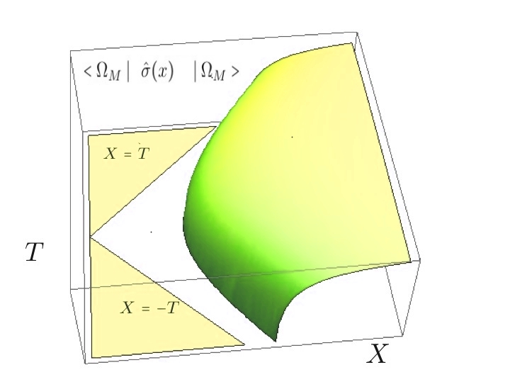
Figure 1: Profile of the Higgs VEV for different points of the space-time as seen by the accelerating observer

V Discussion

The possibility of having symmetry restoration by acceleration, as the one considered in this paper, has been sometimes considered at least controversial because of the following argument (see for example Hill:1985wi ). Let $\sigma_{M}(X)$ be the corresponding classical $\sigma$ field in Minkowski (inertial) coordinates collectively denoted by $X$. Then, as $\sigma$ is an scalar, one should have on the right wedge $\cal R$:

$$\sigma(x)=\sigma_{M}(X)$$ (57)

On the other hand the VEV of the Minkowski quantum field $\hat{\sigma}_{M}(X)$ is given by:

$$<\Omega_{M}\mid\hat{\sigma}_{M}(X)\mid\Omega_{M}>=v.$$ (58)

since the symmetry is spontaneously broken for inertial observers. Is this not in contradiction with the result:

$$<\Omega_{M}\mid\hat{\sigma}(x)\mid\Omega_{M}>=v\sqrt{1-\frac{a^{2}}{a_{c}^{2}}e^{-2ax}}$$ (59)

found in this work? The answer clearly is not, since Eq.(̇57) does not imply that $<\Omega_{M}\mid\hat{\sigma}_{M}(X)\mid\Omega_{M}>$ has to equal $<\Omega_{M}\mid\hat{\sigma}(x)\mid\Omega_{M}>$. The reason is the following: the Minkowski Hilbert space can be split as ${\cal H}_{M}={\cal H}_{L}\otimes{\cal H}_{R}$, where ${\cal H}_{L}$ and ${\cal H}_{R}$ are the Hilbert spaces corresponding to the regions ${\cal L}$ and ${\cal R}$ respectively. $\hat{\sigma}_{M}(X)$ is an operator defined on the whole Minkowski Hilbert space ${\cal H}_{M}$. However $\hat{\sigma}_{R}(x)=\hat{\sigma}(x)$ is an operator defined only on ${\cal H}_{R}$, and it must be understood as $1\otimes\hat{\sigma}_{R}(x)$ when acting on $\mid\Omega_{M}>\in{\cal H}_{M}$. Events belonging to the region ${\cal P}$ can affect events both in ${\cal L}$ and ${\cal R}$. Therefore the field quantum fluctuations in both wedges are entangled and this means that $\hat{\sigma}_{M}$ is not the tensorial product of $\hat{\sigma}_{L}$ and $\hat{\sigma}_{R}$ i.e.:

$$\hat{\sigma}_{M}(X)\neq\theta(-X)\hat{\sigma}_{L}(x)\otimes\theta(X)\hat{\sigma}_{R}(x).$$ (60)

As a consequence Eq.(̇58) and Eq.(̇59) are not incompatible at all.

Another important point concerning our results is the following. Introducing the Unruh like critical temperature:

$$T_{c}=\frac{a_{c}}{2\pi}=2v$$ (61)

and

$$T(x)=\frac{a}{2\pi}e^{-ax}=\frac{1}{2\pi\rho}$$ (62)

the VEV in the comoving frame is given by:

$$<\Omega_{M}\mid\hat{\sigma}(x)\mid\Omega_{M}>=v\sqrt{1-\frac{T(x)^{2}}{T_{c}^{2}}}.$$ (63)

In other words it is like if the Higgs field were feeling a thermal bath with a space-dependent temperature $T(x)$ Candelas:1977zza which diverges at the horizon and goes to zero at the infinite. Notice that this is compatible with the Tolman and Ehrenfest Tolman:1930ona rule for thermal equilibrium in static space-times since:

$$T(x)\sqrt{g_{00}}=T(0)e^{-ax}e^{ax}=\frac{a}{2\pi}$$ (64)

is a $x$ independent constant.

The critical acceleration we have found for the restoration of electroweak symmetry is very large, $a_{c}\simeq 3$ TeV, which is $1.35\times 10^{36}$ m/s², i.e. 35 orders of magnitud larger than the acceleration of gravity on Earth. On the other hand, according to our previous discussion, that means that the phase transition occurs at a distance $\rho\sim 1/a_{c}$ of the horizon which is approximately $0.66\times 10^{-4}$ fm. This is indeed a very small distance and it is difficult to figure out a physical scenario where the phenomenon of electroweak symmetry restoration could take place. However, as commented at the introduction, it is interesting to mention that the LHC is currently studying proton-proton collisions at a center of mass energy of $13$ TeV, which corresponds typically to parton-parton collisions at several TeV’s. Thus it is not discarded that the electroweak symmetry restoration by acceleration considered here could play a role in this kind of processes. Of course a much more detailed analysis is needed but in any case we understand that this physical effect is still interesting from the fundamental point of view.

VI Conclusions

To conclude it is possible to say that the Thermalization Theorem (the Unruh effect) applies to any interacting (not only free) QFT with any kind of fields (scalar, fermionic, gauge, etc) Lee . The Unruh temperature $T=a/2\pi$ is not just a formal artifact but it is a real temperature which can give rise to collective non-trivial phenomena such as phase transitions and symmetry restorations. In particular in this work we have shown how the Unruh effect can produce a restoration of the electroweak $SU(2)_{L}\times U(1)_{Y}$ gauge symmetry of the the SM (inverse Higgs effect). This means that for an accelerating observer the symmetry is restored for accelerations bigger than a critical value $a_{c}=4\pi v\simeq 3$ TeV. For $a>a_{c}$ the electroweak gauge bosons become massless as the photon. Also we have seen that for such an accelerated observer with $a<a_{c}$, the symmetry is also restored beyond a surface defined by $x<x_{c}=\log(a/a_{c})/a$ (in the horizon direction), where the electroweak gauge bosons are massless. In fact this happens also to any other elementary particle (quarks, leptons and the Higgs boson itself) since in the SM all of them have masses controlled by the Higgs VEV. As a consequence all (elementary) particles become massless for enough accelerated observers. We think this is a very interesting result at the fundamental level, coming from the formulation of the SM as a QFT on Rindler space-time. In addition there are some possibilities that it could play a role at the LHC or other higher energy colliders in the future.

ACKNOWLEDGMENTS

The author thanks E. Álvarez and R. Tarrach for triggering our interest in the problem considered in this work, L. Álvarez-Gaumé for comments concerning Bell , C. Pajares for bringing into our attention references Kharzeev:2005iz and DiasdeDeus:2006xk and for useful discussions and J. A. Ruiz-Cembranos for reading the manuscript. Work supported by Spanish grants MINECO:FPA2014-53375-C2-1-P and FPA2016-75654-C2-1-P.

APPENDIX A

Here we will find approximate solutions for the equations Eq. (41) and Eq. (42) to obtain $\bar{\sigma}$ and $\bar{\chi}$. In particular we consider the region $ax<<1$. In this regime the accelerating observer goes into the Minkowski inertial frame for fixed $x$ ($a$ goes to zero) or $x$ goes to zero for fixed $a$. Thus we look for solutions with vanishing $\overline{\chi}$. In Appendix B it is shown how in this case our equations become:

$$0 = \square_{E}\sigma$$ (65)

$$0 = \sigma^{2}-v^{2}+\frac{N}{2\pi^{3}}\int_{0}^{\infty}d\Omega\frac{\Omega\pi}{2\rho^{2}\tanh(\Omega\pi)}.$$ (66)

Introducing $\omega$ as $\omega=a\Omega$ and using $\rho a=1+ax+...$ we find, up to order $ax$:

$$\sigma^{2}=v^{2}-\frac{N}{4\pi^{2}}(1-2ax)\int_{0}^{\infty}d\omega\omega\left(1+\frac{2}{e^{\frac{2\pi}{a}\omega}-1}\right)+...$$

Obviously the first integral requires some regularization and renormalization. This can be done by using a $x$ dependent ultraviolet cutoff $\Lambda e^{-ax}$ and performing the renormalization of the $v$ parameter:

$$v^{2}\rightarrow v^{2}-N\frac{\Lambda^{2}}{2(2\pi)^{2}}(1-2ax+...).$$ (67)

This renormalization naturally matches the $a=0$ limit and is consistent with the red/blue shift detected by the accelerating observer when receiving a signal emitted at the point $x$. Then we have:

$$\sigma^{2}=v^{2}-\frac{N}{2\pi^{2}}(1-2ax)\int_{0}^{\infty}d\omega\omega\frac{1}{e^{\frac{2\pi}{a}\omega}-1}+O((ax)^{2}).$$

By performing the $\omega$ integration, the Minkowski VEV of the $\hat{\sigma}^{2}(x)$ comoving operator is given in the $ax<<1$ regime by:

$$\bar{\sigma}^{2}(x) = <\Omega_{M}\mid(\hat{\sigma}(x))^{2}\mid\Omega_{M}>$$

$$= v^{2}\left(1-\frac{a^{2}N}{12(2\pi)^{2}v^{2}}(1-2ax)\right).$$

By introducing the critical acceleration:

$$a_{c}^{2}=3(4\pi)^{2}\frac{v^{2}}{N}$$ (69)

we have:

$$\bar{\sigma}^{2}(x)=v^{2}\left(1-\frac{a^{2}}{a_{c}^{2}}+2\frac{a^{3}}{a_{c}^{2}}x+...\right).$$ (70)

Notice that at this order this is also a solution of Eq. (41). Therefore, at the origin of the accelerating frame ($x=0$ or $\rho=1/a$), the squared VEV of the $\hat{\sigma}$ field is given by:

$$\bar{\sigma}^{2}(0)=<\Omega_{M}\mid(\hat{\sigma}(0))^{2}\mid\Omega_{M}>=v^{2}\left(1-\frac{a^{2}}{a_{c}^{2}}\right)$$ (71)

for $0\leq a\leq a_{c}$ and clearly:

$$<\Omega_{M}\mid(\hat{\sigma}(0))^{2}\mid\Omega_{M}>=0$$ (72)

for $a>a_{c}$. This is exactly the thermal behavior of the LSM in the large $N$ limit with $a/a_{c}$ playing the role of $T/T_{c}$ (as seen by a inertial observer). It corresponds to a second order phase transition at the critical acceleration $a_{c}$ where the original spontaneously broken symmetry is restored for the accelerating observer.

APPENDIX B

Here we will give some of the details on the computation of the Euclidean Green function $G(x,x^{\prime};s)$ defined by:

$$\left(-\square_{E}\right)_{x}G(x,x^{\prime};s)=\frac{1}{\sqrt{g}}\delta^{(4)}(x-x^{\prime})$$ (73)

for constant $s$ and the appropriate boundary conditions which are periodic in the time coordinate with periodicity $\beta=1/T=2\pi/a$ . We can use Rindler coordinates where:

$$\square_{E}=\partial_{\rho}^{2}+\frac{1}{\rho}\partial_{\rho}+\frac{1}{\rho^{2}}\partial_{\eta}^{2}+\partial_{\bot}^{2}.$$ (74)

Now we introduce the partial Fourier transform:

$$(2\pi)^{2} G(\rho,\rho^{\prime},x_{\bot}-x^{\prime}_{\bot},\eta-\eta^{\prime};s)$$

$$= \sum_{n=-\infty}^{\infty}\int dk_{\bot}^{2}e^{i[n(\eta-\eta^{\prime})+k_{\bot}(x_{\bot}-x^{\prime}_{\bot})]}\tilde{G}(\rho,\rho^{\prime},k_{\bot},n;s)$$

which satisfies:

$$[\rho^{2}\partial_{\rho}^{2}+\rho\partial_{\rho}-(\alpha^{2}\rho^{2}+n^{2})]\tilde{G}=-\rho\delta(\rho-\rho^{\prime})$$ (75)

where $\alpha^{2}=k^{2}_{\bot}+s$. The solution can be written as:

$$\tilde{G}(\rho,\rho^{\prime},k_{\bot},n;s)=\int_{0}^{\infty}d\Omega\frac{\Psi_{\Omega}(\rho)\Psi_{\Omega}(\rho^{\prime})}{\Omega^{2}+n^{2}}$$ (76)

where $\Psi_{\Omega}(\rho)$ can be obtained from the solution of the modified Bessel functions with imaginary parameter:

$$\Psi_{\Omega}(\rho)=\frac{1}{\pi}\sqrt{2\Omega\sinh(\Omega\pi)}K_{i\Omega}(\alpha\rho).$$ (77)

By using well known properties of these functions and:

$$\sum_{n=-\infty}^{\infty}\frac{1}{\Omega^{2}+n^{2}}=\frac{\pi}{\Omega}\frac{1}{\tanh(\Omega\pi)}$$ (78)

it is possible to find:

$$G(x,x;s)=\frac{1}{2\pi^{3}}\int_{0}^{\infty}d\Omega\cosh(\Omega\pi)\int_{0}^{\infty}dkkK_{i\Omega}^{2}(\alpha\rho).$$

Now taking $s=0$ it is straightforward to get Eq. (66).

REFERENCES

REFERENCES

- (1) F. Englert and R. Brout, Phys. Rev. Lett. 13 (1964) 321.
- (2) P. W. Higgs, Phys. Lett. 12 (1964) 132: Phys. Rev. Lett. 13, 508 (1964).
- (3) S.W. Hawking, Nature 248 (1974) 30; Comm. Math. Phys. 43 (1975) 199; Phys. Rev. D14 (1976) 2460.
- (4) W.G. Unruh, Phys. Rev. D14 (1976) 870.
- (5) L. C. B. Crispino, A. Higuchi and G. E. A. Matsas, Rev. Mod. Phys. 80, 787 (2008).
- (6) S. Fulling, Phys. Rev. D7 (1973) 2850: D.G. Boulware, Phys. Rev. D11 (1975) 1404; Phys. Rev. D13 (1976) 2169: L. Parker, Phys. Rev. D12 (1976) 1519: N.D. Birrell and P.C.W. Davies, Quantum fields in curved space (Cambridge University Press, 1982)
- (7) R. Haag, Berlin, Germany: Springer (1992) 356 p. (Texts and monographs in physics)
- (8) R. Kubo, J. Phys. Soc. Jap. 12, 570 (1957): P. C. Martin and J. S. Schwinger, Phys. Rev. 115, 1342 (1959).
- (9) J. Earman, Stud. Hist. Phil. Sci. B 42, 81 (2011).
- (10) J. S. Bell and J. M. Leinaas, Nucl. Phys. B 284, 488 (1987).
- (11) T. D. Lee, Nucl. Phys. B 264, 437 (1986). R. Friedberg, T. D. Lee and Y. Pang, Nucl. Phys. B 276, 549 (1986).
- (12) T. Ohsaku, Phys. Lett. B 599, 102 (2004): D. Ebert and V. C. Zhukovsky, Phys. Lett. B 645 (2007) 267.
- (13) P. Castorina and M. Finocchiaro, J. Mod. Phys. 3 (2012) 1703.
- (14) S. Coleman, Aspects of Symmetry (Cambridge University Press, 1985).
- (15) A. Dobado, “Spontaneous symmetry breaking and the Unruh effect,” in General Relativity, 1916-2016 (Minkowski Institute Press, Montreal 2017). arXiv:1703.05675 [gr-qc].
- (16) D. Kharzeev and K. Tuchin, Nucl. Phys. A 753, 316 (2005).
- (17) J. Dias de Deus and C. Pajares, Phys. Lett. B 642, 455 (2006).
- (18) C. T. Hill, Phys. Lett. 155B, 343 (1985).
- (19) P. Candelas and D. Deutsch, Proc. Roy. Soc. Lond. A 354, 79 (1977).
- (20) R. Tolman and P. Ehrenfest, Phys. Rev. 36, no. 12, 1791 (1930).