Charge reversal and surface charge amplification in asymmetric valence restricted primitive model planar electric double layers in the modified Poisson-Boltzmann theory

Abstract

The modified Poisson-Boltzmann theory of the restricted primitive model double layer is revisited and recast in a fresh, slightly broader perspective. Derivation of relevant equations follow the techniques utilized in the earlier MPB4 and MPB5 formulations and clarifies the relationship between these. The MPB4, MPB5, and a new formulation of the theory are employed in an analysis of the structure and charge reversal phenomenon in asymmetric 2:1/1:2 valence electrolytes. Furthermore, polarization induced surface charge amplification is studied in 3:1/1:3 systems. The results are compared to the corresponding Monte Carlo simulations. The theories are seen to predict the “exact” simulation data to varying degrees of accuracy ranging from qualitative to almost quantitative. The results from a new version of the theory are found to be of comparable accuracy as the MPB5 results in many situations. However, in some cases involving low electrolyte concentrations, theoretical artifacts in the form of un-physical “shoulders” in the singlet ionic distribution functions are observed.

Key words: electric double layer, imaging, restricted primitive model, modified Poisson-Boltzmann theory, Monte Carlo simulations

PACS: 82.45.Fk, 61.20.Qg, 82.45.Gj

Abstract

 ðîáîòi ïåðåãëÿäàєòüñÿ i ïðåäñòàâëÿєòüñÿ ó íîâîìó, áiëüø øèðîêîìó ñâiòëi ìîäèôiêîâàíà òåîðiÿ Ïóàñîíà-Áîëüöìàíà (ÌÒÏÁ) îáìåæåíî¿ ïðèìiòèâíî¿ ìîäåëi ïîäâiéíîãî øàðó. Íà îñíîâi ïîïåðåäíiõ ôîðìóëþâàíü ÌÒÏÁ4 i ÌÒÏÁ5 âèâîäÿòüñÿ âiäïîâiäíi ðiâíÿííÿ, ÿêi äîçâîëÿþòü êðàùå çðîçóìiòè çâ’ÿçîê ìiæ öèìè ôîðìóëþâàííÿìè. ÌÒÏÁ4, ÌÒÏÁ5 i íîâå ôîðìóëþâàííÿ òåîði¿ çàñòîñîâóþòüñÿ äëÿ àíàëiçó ñòðóêòóðè i ÿâèùà çìiíè çíàêó çàðÿäó â åëåêòðîëiòàõ ç àñèìåòðèчíîþ âàëåíòíiñòþ 2:1/1:2. Âèâчàєòüñÿ òàêîæ ÿâèùå iíäóêîâàíîãî ïîëÿðèçàöiєþ çáiëüøåííÿ ïîâåðõíåâî¿ ãóñòèíè çàðÿäó ó ñèñòåìàõ 3:1/1:3. Ïðîâîäèòüñÿ ïîðiâíÿííÿ ç äàíèìè ìîäåëþâàííÿ ìåòîäîì Ìîíòå-Êàðëî. Ïîêàçàíî, ùî íàâåäåíi òåîði¿ âiäòâîðþþòü äàíi ìîäåëþâàííÿ ç ðiçíèì ñòóïåíåì òîчíîñòi âiä ÿêiñíîãî äî ìàéæå êiëüêiñíîãî. Ðåçóëüòàòè íîâîãî âàðiàíòó òåîði¿ â áàãàòüîõ âèïàäêàõ ïðàêòèчíî íå âiäðiçíÿþòüñÿ âiä ðåçóëüòàòiâ ÌÒÏÁ5. Îäíàê ïðè ïåâíèõ óìîâàõ, çîêðåìà ïðè íèçüêèõ êîíöåíòðàöiÿõ åëåêòðîëiòiâ, ñïîñòåðiãàþòüñÿ òåîðåòèчíi àðòåôàêòè ó ôîðìi íåôiçèчíèõ ‘‘ïëåчåé’’ â óíàðíèõ ôóíêöiÿõ ðîçïîäiëó iîíiâ.

Ключовi слова: åëåêòðèчíèé ïîäâiéíèé øàð, âiäîáðàæåííÿ, îáìåæåíà ïðèìiòèâíà ìîäåëü, ìîäèôiêîâàíà òåîðiÿ Ïóàñîíà-Áîëüöìàíà, ìîäåëþâàííÿ Ìîíòå-Êàðëî

1 Introduction

Electric double layers play a key role in a wide variety of phenomena, in the fields diverse as colloids, physical and biological systems, and electrochemistry [1, 2, 3, 4, 5, 6, 7, 8]. Recent years have seen an increasing relevance of double layers in DNA sequencing [9, 10], drug delivery [11, 12], and green technology, viz., designing novel energy storage devices as in super-capacitors (see for example, reference [13]). An electric double layer appears when a system of charged particles in a fluid is in the neighborhood of a charged surface. Various models and theories have been developed depending upon the physical system being treated. A simple model of an electrolyte next to a plane charged surface is a basic model in many areas. Gouy and Chapman [14, 15] analysed this model, based on the Poisson-Boltzmann (PB) equation, where the electrolyte was treated as a system of point ions moving in a medium of constant permittivity. Later on, Stern [16] proposed to lower the permittivity in the region immediately next to the planar electrode (Stern layer) in order to bring the computed double layer capacitance in line with the experiments. At not too high surface charge and electrolyte concentration for univalent ions, the Gouy-Chapman-Stern (GCS) theory describes reasonably well the diffuse part of the electric double layer. However, double layer research over the last four decades involving formal statistical mechanical theories, simulations, and experiments has shown the shortcomings of the theory in capturing many physical phenomena (see for example, the review [8]). As a case in point, the GCS theory cannot explain the two phenomena that are the focus of this work, namely, charge reversal (CR) (or charge inversion or overcharging) and surface charge amplification (SCA). In CR, the local density of the counterions overcompensate the surface charge, while in SCA, in the absence of specific ion adsorption, there is an apparent increase in the surface charge due to an excess of coions.

CR was indicated in the simulation work of Torrie and Valleau [17, 18], Snook and van Megen [19] and in the modified Poisson-Boltzmann (MPB) and hypernetted-chain/mean spherical approximation (HNC/MSA) theories [20]. The important feature of these works was allowing the ions to have size and accounting for the approximations in the PB equation. There is now a large body of theoretical and experimental work on charge reversal in colloidal systems due to its importance in both equilibrium and non-equilibrium situations [1, 2, 21, 22, 23, 24, 25, 26, 27, 28, 29]. Surface charge amplification is more counterintuitive than CR. It can occur when the ions have asymmetry in size and charge [30, 31, 32, 33, 34]. Imaging can also promote SCA, even when the ions are of equal size [35, 36, 37]. Here, we discuss the MPB theory with imaging for equisized ions with 1:2/2:1, 1:3/3:1 electrolytes.

2 Model and theory

The electric double layer is modelled by a restricted primitive model electrolyte in the neighborhood of a uniformly charged plane electrode. The solute molecules are hard spheres of diameter $a$ with point charges at their center moving in a medium of constant relative permittivity $\epsilon_{r}$, while the electrode has a constant relative permittivity of $\epsilon_{\text{w}}$. The analysis presented here builds upon the earlier formulations of MPB4 [38, 39] and MPB5 [40] versions of the theory and clarifies the relation between them. The present approach is a bit more general since the MPB5 situation will be seen to follow as a special limiting case. The connections to the MPB4 are also explored.

At a perpendicular distance $x$ from the electrode into the solution, the mean electrostatic potential $\psi(x)$ satisfies Poisson’s equation

$$\frac{\mathrm{d}^{2}\psi}{\mathrm{d}x^{2}}=-\frac{1}{\epsilon_{0}\epsilon_{r}}\sum_{s}e_{s}n_{s}g_{s}(x),$$ (1)

where the sum is over the ion species, $\epsilon_{0}$ is the vacuum permittivity, $e_{s}$ is the charge of an ion of species $s$, $n_{s}$ and $g_{s}(x)$ are the mean number density and singlet distribution function for an ion of species $s$, respectively. Kirkwood’s charging process [41] for an ion $i$ at $x_{1}$ gives

$$g_{i}(x_{1})=\zeta_{i}(x_{1})\exp\Bigg{[}-\beta e_{i}\psi(x_{1})-\beta\int_{0}^{e_{i}}\lim_{r\rightarrow 0}(\phi_{i}^{*}-\phi_{i\text{b}}^{*})\mathrm{d}e_{i}\Bigg{]},$$ (2)

where

$$\phi_{i}^{*}=\phi_{i}(1;2)-\frac{e_{i}}{4\piup\epsilon_{0}\epsilon_{r}r}$$ (3)

with $\phi_{i\text{b}}^{*}$ being the bulk value of $\phi_{i}^{*}$. Here, $\zeta_{i}(x_{1})=g_{i}(x_{1}/e_{i}=0)$ is the exclusion volume term, $\phi_{i}=\phi_{i}(1;2)$ is the fluctuation potential at ${\bf r}_{2}$ for an ion at ${\bf r}_{1}$, $r=r_{12}$, and $\beta=1/(k_{\text{B}}T)$ ($k_{\text{B}}$ is the Boltzmann’s constant and $T$ is the absolute temperature).

The fluctuation potential can be shown to satisfy the following set of differential equations [40]

$$\nabla^{2}\phi_{i} =0,\hskip 50.58878ptx<a/2,$$ (4)

$$\nabla^{2}\phi_{i} =-\frac{\mathrm{d}^{2}\phi_{i}}{\mathrm{d}x^{2}}\,,\hskip 27.46295ptr<a,$$ (5)

$$\nabla^{2}\phi_{i} =\kappa^{2}(x)\phi_{i}\,,\hskip 23.48752ptx>a/2,~{}~{}r>a,$$ (6)

where $x=x_{2}$ and $\kappa(x)$ is the local Debye-Hückel parameter defined by

$$\kappa^{2}(x)=\frac{\beta}{\epsilon_{0}\epsilon_{r}}\sum_{s}e_{s}^{2}n_{s}g_{s}(x).$$ (7)

Equations (4) and (5) are exact, while equation (6) involves two approximations. These are Loeb’s closure [42], which gives a closed system of equations for $\phi_{i}$, and the linearization of the equation involving Loeb’s closure. The boundary conditions associated with equations (4)–(6) are $\phi_{i}$ and $\partial\phi_{i}/\partial n$ continuous ($n$ denotes normal) at $x=a/2$ and $r=a$, while at the electrode $\phi_{i}$ is continuous but $\epsilon_{r}\partial\phi_{i}/\partial x^{+}=\epsilon_{\text{w}}\partial\phi_{i}/\partial x^{-}$. Approximate solutions of equations (4)–(6) have been considered for both point ions [43] and finite size ions [40]. The point ion solution suggests an appropriate solution in the regions $x<0$, $0<x<a/2$. From the analysis of reference [43], the limiting case of having no distance of closest approach and $k\rightarrow 0$ gives

$$\phi_{i} =\frac{e_{i}}{4\piup\epsilon_{0}\epsilon_{r}r}(1+f),\hskip 27.46295ptx<0,$$ (8)

$$\phi_{i} =\frac{e_{i}}{4\piup\epsilon_{0}\epsilon_{r}}\left(\frac{1}{r}+\frac{f}{r^{*}}\right),\qquad x>0,$$ (9)

where $f=(\epsilon_{r}-\epsilon_{\text{w}})/(\epsilon_{r}+\epsilon_{\text{w}})$ and $r^{*}$ is the distance of the image of $e_{i}$ in the electrode from the field point. These two results suggest that an appropriate approximation for the ion size result for the equation (4) is

$$\phi_{i} =C\left(\frac{1}{r}+\frac{f}{r}\right),\qquad x<0,$$ (10)

$$\phi_{i} =C\left(\frac{1}{r}+\frac{f}{r^{*}}\right),\qquad 0<x<a/2,$$ (11)

which were used in reference [40].

Previous work [38, 40, 44, 45, 46, 47] has shown that a good approximation to the solution of equation (6) is

$$\phi_{i}=B\frac{\exp(-\kappa r)}{r}+B^{*}\frac{\exp(-\kappa r^{*})}{r^{*}}\,,\qquad x>a/2,~{}r>a,$$ (12)

where $\kappa=\kappa(x_{1})$. The point ion result, with a distance of closest approach, indicates a complex situation such that $B$, $B^{*}$, $C$ can contain the imaging factor $f$.

The use of the approximate solutions (10)–(12) mean that the boundary conditions cannot be satisfied. An approximate fitting of the boundary conditions was considered in [40], giving the MPB5 theory. Here, we adopt the approach of reference [38]. The application of Green’s second identity to $\phi_{i}^{*}$ and $1/r$ in the exclusion sphere $V$, where $V$ is a truncated sphere if $a/2<x<3a/2$, gives, on using equation (5)

$$4\piup\lim_{r\rightarrow 0}\phi_{i}^{*} =\int_{V}\left(\frac{1}{r}-\frac{1}{a}\right)\nabla^{2}\psi\mathrm{d}V+\frac{1}{a^{2}}\int_{S_{\text{I}}}\phi_{i}\mathrm{d}S-\frac{1}{a}\int_{S_{\text{W}}}\frac{\partial\phi_{i}}{\partial n}\mathrm{d}S$$

$$\quad+\int_{S_{\text{W}}}\left[\frac{1}{r}\frac{\partial\phi_{i}}{\partial n}-\phi_{i}\frac{\partial}{\partial n}\left(\frac{1}{r}\right)\right]\mathrm{d}S-\frac{e_{i}}{a\epsilon_{0}\epsilon_{r}}\,.$$ (13)

Here, $S_{\text{W}}$ and $S_{\text{I}}$ are respectively the wall and double layer surface portions of the truncated sphere. The integrals over $S_{\text{W}}$ vanish for $x>3a/2$, and $S_{\text{I}}$ is then the complete spherical surface. For reference, the values of the integrals appearing in equation (13), using the approximations for $\phi_{i}$, are given in the appendix.

To determine the relations between $B$, $B^{*}$ and $C$ we use Gauss’s theorem for ion $i$

$$\int_{S}\frac{\partial\phi_{i}}{\partial n}\mathrm{d}S=-\frac{e_{i}}{\epsilon_{0}\epsilon_{r}}-\int_{V}\nabla^{2}\psi\mathrm{d}V.$$ (14)

Thus, combining the expressions resulting from the evaluation of equations (13), (14) with equation (2) gives

$$g_{i}(x) =\zeta_{i}(x)\exp\Bigg{\{}-\frac{1}{2}\beta e_{i}\Bigg{[}\left(\frac{e_{i}}{4\piup\epsilon_{0}\epsilon_{r}}\right)(F-F_{0})+F\psi(x+a)+F\psi(x-a)$$

$$\quad-\frac{(F-1)}{a}\int_{x-a}^{x+a}\psi(X)\mathrm{d}X\Bigg{]}\Bigg{\}},$$ (15)

where for $a/2<x<3a/2$

$$F =\frac{A}{D}\,,$$ (16)

$$A =(2x+a)\mathrm{e}^{-y}+\frac{C}{B}(3a-2x)+\frac{C}{B}\frac{af}{x}(a-2x+s)+\frac{a}{\kappa x}\frac{B^{*}}{B}\left[\mathrm{e}^{-\kappa s}-\mathrm{e}^{-\kappa(2x+a)}\right],$$ (17)

$$D =(1+y)(2x+a)\mathrm{e}^{-y}+\frac{C}{B}(3a-2x)+\frac{C}{B}f(s-2a)-\frac{a}{\kappa x}\frac{B^{*}}{B}\Big{[}(1+y)\mathrm{e}^{-\kappa(2x+a)}$$

$$\quad-\frac{1}{a}(a+\kappa sa-\kappa sx)\mathrm{e}^{-\kappa s}\Big{]}$$ (18)

and for $x>3a/2$

$$F=\frac{1+\frac{1}{2\kappa x}\left(\frac{B^{*}}{B}\right)\mathrm{e}^{-\kappa(2x-a)}\sinh y}{1+y-\frac{1}{2\kappa x}\left(\frac{B^{*}}{B}\right)\mathrm{e}^{-\kappa(2x-a)}(y\cosh y-\sinh y)}\,,$$ (19)

where $F_{0}=\lim_{x\rightarrow\infty}F$, $y=\kappa a$ and $s=\sqrt{a^{2}+2xa}$.

At $x=3a/2$, we have that $F$ is continuous but $\partial F/\partial x$ is discontinuous in general. The expression for $F$ depends upon the ratios $C/B$, $B^{*}/B$ for $a/2<x<3a/2$ and on the single ratio $B^{*}/B$ for $x>3a/2$. Putting $C=B\exp(-y)$, $B^{*}=Bf\exp(-y+\kappa s)$ in $a/2<x<3a/2$ and $B^{*}=Bf\exp y$ in $x>3a/2$ gives the MPB5 theory [40]. Early calculations of $F$ did not consider the exclusion region $0<x<a/2$ for $\phi_{i}$ so that $F$ is defined in the two regions $a/2<x<a$ and $x>a$, for example the MPB4 theory [38, 39]. In these earlier works, the value of $F$ differs from that of the MPB5 when $x>3a/2$. On putting $B^{*}=fB$ in equation (19), the $F$ of MPB4 for $x>a$ is derived. This suggests an alternative $F$, analogous to that for MPB4, which is given by $C=B$ in equations (17), (18) and $B^{*}=fB$ in equations (17)–(19). There are many possibilities of choosing the ratios $C/B$, $B^{*}/B$, depending upon the chosen criterion. However, a better approach may be to improve upon the analysis of equations (4), (5) and the nonlinear version of equation (6).

Various expressions have been used for evaluating the exclusion volume term $\zeta_{i}(x)$ in equation (2) [38, 39, 48]. The most accurate exclusion volume terms are those based on the BBGY expansion [39] or charging up the wall and introducing the non-uniform direct correlation function [48]. Here, we will use the BBGY approach, where for $x>a/2$

$$\zeta_{i}(x)=\exp\left\{-2\piup\int_{\infty}^{x}\sum_{s}n_{s}\zeta_{is}(a)\int_{\text{max}(\frac{a}{2},y-a)}^{y+a}(X-y)g_{s}(X)\exp[-\beta e_{i}\Phi(y,X)]\mathrm{d}X\mathrm{d}y\right\}$$ (20)

with $\zeta_{i}(x)=0$ for $x<a/2$. The contact value $\zeta_{ij}(a)$ between ions $i$ and $j$ is that proposed by Fischer [49] while $\Phi(y,X)=\phi(1;2/e_{s}=0/r_{12}=a)$.

2.1 Monte Carlo simulations

The Monte Carlo simulations were performed in the canonical ($N,V,T$) ensemble using the standard and widely used Metropolis algorithm [50, 51]. The techniques were the same as those used in some of our earlier works (see for example, references [52, 53]). The MC cell was a rectangular parallelepiped of dimensions $L_{x}$, $L_{y}$, and $L_{z}$, with $L_{y}=L_{z}$. One of the $y$-$z$ faces was a charged wall, viz., the electrode with a uniformly distributed surface charge at $x=0$, while the other at $x=L_{x}$ was a neutral wall. The surface charge density on the electrode was determined from

$$\sigma=-\frac{(N_{+}|Z_{+}|-N_{-}|Z_{-}|)e}{L_{y}^{2}}\,,$$ (21)

where $N_{+}$ and $N_{-}$ are the number of cations and anions, respectively. It is to be noted that with the above definition of $\sigma$, the local electro-neutrality at the wall is built in. In order to simulate the semi-infinite system, conventional minimum image techniques along with periodic boundary conditions in the $y$ and $z$ directions were implemented [51]. The effect of the long range nature of the Coulomb interactions was treated by the parallel charge sheets method pioneered by Torrie and Valleau [17]. This procedure was later examined and improved upon by Boda et al. [54], who also confirmed the validity of the method for charge hard spheres.

The situation when the permittivity of the medium of the charged wall differs from that of the electrolyte solution has also been treated by Torrie at al. [55] and their procedure adopted here. These authors regarded the polarizability of the electrode as a classic electrostatic image problem, viz., the total surface charge density $\sigma$ has a contribution from the fictitious image charge $-f\sigma$ due to the polarization of the electrode. In passing we would like to note that the Torrie and co-workers did their simulations in the grand canonical ($\mu,V,T$) ensemble unlike the canonical ensemble in the present case.

In the canonical ensemble, the bulk target concentration can only be achieved by a trial-and-error method of adjusting the cell length $L_{x}$ and/or the number of particles. We used both of these methods where necessary and imposed a tolerance of less than 2$\%$ error in reproducing the bulk concentration. Typically, around 400 particles were simulated and approximately $10^{8}$ configurations sampled out of which the first $10^{7}$ (10$\%$ of the total number of configurations) were used for system equilibration before statistics were taken.

3 Results

The properties of the diffuse double layer are found by solving the Poisson equation, equations (1) and (15), for the mean electrostatic potential and hence from equation (15) the singlet distribution function. Three different values of $F$ were treated in detail, these corresponding to those of MPB4, MPB5, and the new $F$ given by $C=B$, $B^{*}=fB$ in equations (16)–(19), respectively. A quasi-linearisation technique was used [38, 56] which has been successfully employed in past investigations. The parameters chosen were those used by Wang [37] who simulated charge asymmetric 1:3 and 3:1 RPM electrolytes with imaging. For the RPM electrolyte, we treat 1:2, 2:1 and some 1:3, 3:1 valences with $a=4\cdot 10^{-10}$ m, $\epsilon_{r}=80$, $T=298$ K while the wall is characterized by $\epsilon_{\text{w}}=2,80$ or $\infty$. When $\epsilon_{\text{w}}\neq\epsilon_{r}$, imaging occurs which is repulsive for $\epsilon_{\text{w}}<\epsilon_{r}$ and attractive for $\epsilon_{\text{w}}>\epsilon_{r}$. The value $\epsilon_{\text{w}}=$ 2, which is relevant for a medium such as silica, while $\epsilon_{\text{w}}=\infty$ represents a metallic electrode.

We start by looking in detail at the predictions of the MPB5 theory for 2:1 electrolytes with and without imaging. Figures 2 and 2 treat the repulsive ($f=0.9513$) and attractive ($f=-1$) cases, respectively, at electrolyte concentration $c=0.24$ mol/dm³ and surface charge density $\sigma=-0.02$ C/m². Displayed are the singlet distribution functions $g_{s}(x/a)$, the dimensionless mean electrostatic potential $\psi^{*}(x/a)=|e|\beta\psi(x/a)$ and the integrated charge density $q(x/a)$ defined by

$$q(x)=\sigma+\sum_{s}n_{s}e_{s}\int_{0}^{x}g_{s}(y)\mathrm{d}y.$$ (22)

The integrated charge gives a measure of the total charge within a distance $x$ of the electrolyte and enables a succinct illustration of the two phenomena CR and SCA.

Figure 1: (Color online) The MPB5 electrode-ion singlet distribution functions $g_{s}(x/a)$ (lower panel), the mean electrostatic potential $\psi^{*}(x/a)$ (middle panel), and the integrated charge $q(x/a)$ (upper panel) as functions of $x/a$ for a 2:1 electrolyte. The symbols represent MC data, while the lines represent the MPB results. The notations “co” and “cntr” stand for “coion” and “counterion”, respectively. Legend as given in the figure.

Figure 2: (Color online) The MPB5 electrode-ion singlet distribution functions $g_{s}(x/a)$ (lower panel), the mean electrostatic potential $\psi^{*}(x/a)$ (middle panel), and the integrated charge $q(x/a)$ (upper panel) as functions of $x/a$ for a 2:1 electrolyte. Notation as in figure 2 and legend as given in the figure.

For no imaging, the simulated singlet distribution functions apparently display a monotonous behaviour of the co and counter ions, with a corresponding monotonous behaviour of the mean electrostatic potential and the integrated charge. The MPB5 theory has a small shoulder in the counterion $g_{s}(x)$ at $x\sim 3a/2$ arising from the discontinuity of $\partial F/\partial x$ at $x=3a/2$. This is an unfortunate feature at low concentrations which has been observed earlier [40]. The influence of this feature is not observed in $\psi^{*}(x)$ since $\psi^{*}(x)$ and its derivative are continuous everywhere. The principal effect of imaging in the distribution functions for the repulsive situation is that the divalent counterion is attracted for large $x$ but reduces and becomes small near the wall, while a slight reduction is seen in the monovalent coion. Conversely for the attractive situation, the coion profile increases to a value greater than 1 near the electrode, and the counterion profile rapidly increases in the neighborhood of the electrode. These imaging effects are reflected in the reduction (repulsive case) and increase (attractive case) over the no imaging situation, of the mean electrostatic potential and integrated charge. A very small CR is seen when $f=-1$. The MPB5 accurately predicts $\psi^{*}(x)$ and $q(x)$, and apart from the shoulder feature, the $g_{s}(x)$ are quantitatively or qualitatively correct.

Figure 3: (Color online) The MPB5 electrode-ion singlet distribution functions $g_{s}(x/a)$ (lower panel), the mean electrostatic potential $\psi^{*}(x/a)$ (middle panel), and the integrated charge $q(x/a)$ (upper panel) as functions of $x/a$ for a 2:1 electrolyte. Notation as in figure 2 and legend as given in the figure.

Figure 4: (Color online) The MPB5 electrode-ion singlet distribution functions $g_{s}(x/a)$ (lower panel), the mean electrostatic potential $\psi^{*}(x/a)$ (middle panel), and the integrated charge $q(x/a)$ (upper panel) as functions of $x/a$ for a 2:1 electrolyte. Notation as in figure 2 and legend as given in the figure.

At the higher concentration $c=1$ mol/dm³ and surface charge $\sigma=-0.2$ C/m², there is a clear change in the electrolyte properties, viz., figures 4, 4. The striking feature is the obvious damped oscillatory behaviour of various functions for all three situations ($f=0.9513$, $f=0$, $f=-1$). The onset of this oscillatory behaviour mainly depends, at a small surface charge, upon the value of $y_{0}=\kappa_{0}a$, where $\kappa_{0}$ is the bulk Debye-Hückel constant. A damped oscillatory behaviour in $\psi^{*}(x)$ is predicted in the linear MPB theory for $y_{0}>$ 1.2412 [57] for symmetric valences and for $y_{0}>$ 1.15 [45] for 2:1/1:2 valences. However, the latter is probably too high since in simulation and the HNC, the $g_{s}(x)$ value for 1:2 homogeneous electrolytes implies $y_{0}\approx 0.76$ [58]. Here, $y_{0}=2.26$, while the previous concentration of 0.24 mol/dm³ gave $y_{0}=1.11$, so that a qualitative change in the behaviour between the two concentrations is predicted by the MPB theories. With no imaging, the initial maximum in $\psi^{*}(x)$ is at $x\sim a$ with CR starting at about the same value of $x$ and having a maximum at $x\sim 5a/4$. Both the repulsive and attractive cases are qualitatively similar to that for no imaging, showing small but different deviations from $f=0$. For example, with the mean potential, the first maximum is shifted to a larger $x$ for the repulsive case, but closer to the electrode with a larger maximum for the attractive case. At this higher concentration, there is no shoulder in the MPB5 $g_{s}(x)$ at $x\sim 3a/2$, and the MPB5 gives an accurate picture of all three functions. Clearly, the effect of discontinuity in $\partial F/\partial x$ at $x=3a/2$ gets masked at high concentrations. The MPB4 theory seems a possible alternative to the MPB5 theory as it does not have this discontinuity at $x=3a/2$. Figures 6 and 6 show the MPB4 for the 2:1 attractive cases. Clearly, the theory is inadequate, especially for the lower concentration. The main inaccuracy is the unphysical upturn in the coion distribution function close to the wall. A further possible alternative theory is that given by $C=B$, $B*=fB$ in equations (16)–(19). Looking again at the 2:1 attractive cases, figures 8 and 8, this theory incorrectly predicts (i) an unphysical rise in the coion $g_{s}(x)$ near the wall, (ii) a shoulder in the counterion $g_{s}(x)$ for no imaging at the lower concentration. Apart from the unphysical behaviour (i), the theory based on the new $F$ gives a good representation of the mean potential and integrated charge at $c=1$ mol/dm³. Unfortunately, neither the MPB4 nor that based on the new $F$ is an improvement on the MPB5.

Figure 5: (Color online) The MPB4 electrode-ion singlet distribution functions $g_{s}(x/a)$ (lower panel), the mean electrostatic potential $\psi^{*}(x/a)$ (middle panel), and the integrated charge $q(x/a)$ (upper panel) as functions of $x/a$ for a 2:1 electrolyte. Notation as in figure 2 and legend as given in the figure.

Figure 6: (Color online) The MPB4 electrode-ion singlet distribution functions $g_{s}(x/a)$ (lower panel), the mean electrostatic potential $\psi^{*}(x/a)$ (middle panel), and the integrated charge $q(x/a)$ (upper panel) as functions of $x/a$ for a 2:1 electrolyte. Notation as in figure 2 and legend as given in the figure.

Figure 7: (Color online) The MPB (new $F$) electrode-ion singlet distribution functions $g_{s}(x/a)$ (lower panel), the mean electrostatic potential $\psi^{*}(x/a)$ (middle panel), and the integrated charge $q(x/a)$ (upper panel) as functions of $x/a$ for a 2:1 electrolyte. Notation as in figure 2 and legend as given in the figure.

Figure 8: (Color online) The MPB5 and MPB (new $F$) electrode-ion singlet distribution functions $g_{s}(x/a)$ (lower panel), the mean electrostatic potential $\psi^{*}(x/a)$ (middle panel), and the integrated charge $q(x/a)$ (upper panel) as functions of $x/a$ for a 2:1 electrolyte. Notation as in figure 2 and legend as given in the figure.

Figure 9: (Color online) The MPB5 electrode-ion singlet distribution functions $g_{s}(x/a)$ (lower panel), the mean electrostatic potential $\psi^{*}(x/a)$ (middle panel), and the integrated charge $q(x/a)$ (upper panel) as functions of $x/a$ for a 1:2 electrolyte. Notation as in figure 2 and legend as given in the figure.

Figure 10: (Color online) The MPB5 electrode-ion singlet distribution functions $g_{s}(x/a)$ (lower panel), the mean electrostatic potential $\psi^{*}(x/a)$ (middle panel), and the integrated charge $q(x/a)$ (upper panel) as functions of $x/a$ for a 1:2 electrolyte. Notation as in figure 2 and legend as given in the figure.

Figures 10 and 10 consider the prediction of the MPB5 theory for the 1:2 electrolyte where now the coion is divalent. Counterion attraction with the wall plays a dominant role in shaping the structural properties of the electric double layer and hence many of the 1:2 double layer properties are similar to those of the 1:1 case, while the 2:1 properties resemble that for the 2:2 situation (see for example, reference [59]). Thus, it comes as no surprise that the predicted structure for the 1:2 cases are relatively closer to the simulations than that seen earlier for the 2:1 cases. Only attractive imaging is treated in figures 10, 10 since any deviation from no imaging tends to be greater than those for the repulsive case. At a low concentration, figure 10, the coion is attracted near the wall, and since it is divalent, it has a greater contact value than in the monovalent case in figure 2. The difference in the valence of the counterion means that the deviations from no imaging for the mean potential and an integrated charge are less and oppositely directed. At a higher concentration, figure 10, the imaging has little effect. There is still a damped oscillatory feature in the functions, with CR occurring, but it is not as pronounced as for the divalent counterion. Overall, the MPB5 theory accurately predicts the 1:2 double layer, apart from the behaviour of the coion in the neighborhood of $x=3a/2$. The alternative MPB4 and new $F$ theories perform well in the 1:2 case.

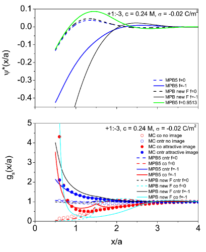
Figure 11: (Color online) The MPB5 and MPB (new $F$) electrode-ion singlet distribution functions $g_{s}(x/a)$ (lower panel) and the mean electrostatic potential $\psi^{*}(x/a)$ (upper panel) as functions of $x/a$ for a 1:3 electrolyte. Notation as in figure 2 and legend as given in the figure. The MC data are from reference [37].

Figure 12: (Color online) The MPB5 and MPB (new $F$) integrated charge $q(x/a)$ as a function of $x/a$ for a 1:3 electrolyte. The symbols represent MC data, while the lines represent the MPB results. Legend as given in the figure. The MC data are from reference [37].

Figure 13: (Color online) The MPB5 integrated charge $q(x/a)$ as a function of $x/a$ for a 3:1 electrolyte. The symbols represent MC data, while the lines represent the MPB results. Legend as given in the figure. The MC data are from reference [37].

Lastly, we briefly look at the MPB theory for a 1:3 and 3:1 electrolyte with the imaging at $c=0.24$ mol/dm³ and $\sigma=-0.02$ C/m². Replacing the divalent coion by a trivalent ion leads to CR ($f=0.9513$, $f=0$) and also to SCA when there is an attractive imaging ($f=-1$), viz., figures 11, 13. Alternatively, when the trivalent ion is the counterion there is again CR and SCA, but now SCA occurs when there is a repulsive imaging and CR for an attractive imaging, viz., figure 13. MC simulations [37] indicate that the MPB5 prediction of SCA for no imaging is incorrect. The CR is expected as $y_{0}=1.5636$, while the counterintuitive SCA arises solely through polarization forces. In the 1:3 situation, the attraction of the coion image overcomes the repulsion of the surface charge, while for the 3:1 electrolyte, a much larger repulsive force acting on the counterion is sufficient to neutralise the screening in the neighborhood of the wall. SCA does not occur for either 1:2 or 2:1 electrolytes at these parameters. Higher valences provide a stringent test for theories. The discrepancies in $g_{s}(x)$ mean that the MPB5 and the new $F$ theory predict both CR and SCA with varying degrees of success.

4 Conclusions

In this paper, we have looked again at the formulation of a modified Poisson-Boltzmann equation for the planar electric double layer formed by a restricted primitive model electrolyte. The derivation of the MPB equation follows the pattern and techniques utilized in some of our earlier works [38, 39] but is a bit more general. Our focus was on obtaining a general expression for the quantity $F$, a key ingredient in the theory, which incorporates important aspects of inter-ionic correlations. We have shown that an earlier version of the theory, viz., MPB5 [40], follows as a special case of the generalized $F$. Although the MPB4 version does not follow directly, the relationship between these two versions can be clearly assessed. With such features built in, the theory is more flexible and it is likely that the MPB equation will become more adaptable to particular physical situations.

The MPB theory does not satisfy exactly the contact condition [60, 61, 62] which holds for no imaging. Previous work [63, 64, 65] has shown that the MPB5 theory fairly accurately satisfies the contact condition for 1:1 electrolytes and gives a good agreement for 1:2/2:1 and 2:2 electrolytes. A similar conclusion holds in general when the new $F$ is used, but the MPB4 theory can be poor. Adapting the MPB approach to satisfy the contact condition would be useful for inner consistency. However, for the present univalent and divalent RPM electrolytes, the MPB5 theory has shown to be in good overall agreement with both structural and thermodynamic simulation properties [59].

We have studied the effect of imaging on 1:2, 2:1 valence electrolytes with the emphasis on the phenomenon of charge reversal. Also briefly treated were 1:3, 3:1 electrolytes where, besides the charge inversion, polarization can produce the counterintuitive surface charge amplification. The conclusions are mainly twofold:

(a) structural and charge reversal behaviour are generally well described by the various MPB theories compared to MC simulations. For the 1:3, 3:1 systems, the theories are poor relative to the 1:2, 2:1 cases, which is not unexpected at the higher multi-valence situations. Furthermore, the theoretical predictions tend to be closer to the simulation data for monovalent counterions rather than for multivalent counterions, a feature that is well known in the double layer literature.

(b) The new formulation of $F$ allows for different choices to be made for $F$. One of the new $F$’s analyzed gives reasonable results that in some situations are at a par with MPB5. However, there are issues, the main one being the appearance of an nonphysical shoulder in the singlet distribution functions at lower concentrations, similar to that seen in MPB5.

The shoulders are artifacts of the theory, which come from discontinuities in the slope of the fluctuation potential $\phi$ at $x=3a/2$. In the analysis outlined, although $\phi$ is continuous across the planar surface of the truncated exclusion sphere (cf. section 2), the normal derivative is not continuous. The continuity of the normal derivative may well be achieved by an appropriate choice of $B$, $B^{*}$, $C$ in equations 16, 19. It is to be seen if such choices in the present approach will give a simple means of eliminating the shoulder in the distribution function. Further analytic work along the lines of MPB5 may be difficult, so that eventually the best approach may well be a numerical evaluation of the fluctuation potential.

Appendix

Evaluation of the integrals in equations (13), (14) using the expressions (11) and (12) for the fluctuation potential $\phi_{i}$ in $a/2<x<3a/2$

$$\int_{S_{\text{I}}}\phi\mathrm{d}S=\piup\left\{B(2x+a)\mathrm{e}^{-y}+\frac{aB^{*}}{\kappa x}\left[\mathrm{e}^{-\kappa s}-\mathrm{e}^{-\kappa(2x+a)}\right]\right\},$$ (23)

$$\int_{S_{\text{W}}}\frac{\partial\phi}{\partial n}\mathrm{d}S=\piup C\left[\frac{2x-3a}{a}+\frac{2f}{s}\left(s-x-\frac{a}{2}\right)\right],$$ (24)

$$\int_{S_{\text{W}}}\left[\frac{1}{r}\frac{\partial\phi}{\partial n}-\phi\frac{\partial}{\partial n}\left(\frac{1}{r}\right)\right]\mathrm{d}S=\frac{\piup Cf}{xas}\left(a^{2}-2x^{2}+ax+as\right),$$ (25)

$$\int_{S_{\text{I}}}\frac{\partial\phi}{\partial n}\mathrm{d}S=\piup\left\{-\frac{B}{a}(1+y)(2x+a)\mathrm{e}^{-y}+\left(\frac{B^{*}}{\kappa x}\right)\left[(1+y)\mathrm{e}^{-\kappa(2x+a)}-\left(\frac{1}{a}\right)(a+ys-\kappa sx)\mathrm{e}^{-\kappa s}\right]\right\}$$ (26)

and in $x>3a/2$

$$\int_{S}\frac{\partial\phi}{\partial n}\mathrm{d}S=2\piup\left[-2B(1+y)\mathrm{e}^{-y}+\left(\frac{B^{*}\mathrm{e}^{-2\kappa x}}{\kappa x}\right)(y\cosh y-\sinh y)\right],$$ (27)

$$\int_{S}\phi\mathrm{d}S=2\piup a\left[2B\mathrm{e}^{-y}+\left(\frac{B^{*}\mathrm{e}^{-2\kappa x}}{\kappa x}\right)\sinh y\right].$$ (28)

The mean electrostatic potential integrals are

$$\int_{V}\nabla^{2}\psi\mathrm{d}V=2\piup a\Bigg{[}\psi(x+a)+\psi(x-a)-\frac{1}{a}\int_{x-a}^{x+a}\psi(X)\mathrm{d}X\Bigg{]},$$ (29)

$$\int_{V}\frac{\nabla^{2}\psi}{r}\mathrm{d}V=2\piup\left[\psi(x+a)+\psi(x-a)-2\psi(x)\right],$$ (30)

which for a truncated sphere are to be evaluated in conjunction with the linear result in $0<x<a/2$,

$$\psi(x)=\psi(0)+x\left[\frac{\mathrm{d}\psi}{\mathrm{d}x}\right]_{x=0}.$$ (31)

Ukrainian 0 Çìiíà çíàêó i çáiëüøåííÿ ïîâåðõíåâî¿ ãóñòèíè çàðÿäó ó âàëåíòíî-àñèìåòðèчíié îáìåæåíié ïðèìiòèâíié ìîäåëi ïëàíàðíèõ åëåêòðèчíèõ ïîäâiéíèõ øàðiâ â ðàìêàõ ìîäèôiêîâàíî¿ òåîði¿ Ïóàñîíà-Áîëüöìàíà

Ë.Á. Áóÿí${}^{\textsf{\footnotesize{\mbox{?}}}}$, Ê.Ó. Àóòâåéò${}^{\textsf{\footnotesize{\mbox{?}}}}$

             
${}^{\textsf{\footnotesize 1}}$ Ëàáîðàòîðiÿ òåîðåòèчíî¿ ôiçèêè, âiääië ôiçèêè, À/ñ 70377, Óíiâåðñèòåò Ïóåðòî-Ðiêî, Ñàí Õóàí, Ïóåðòî-Ðiêî ${}^{\textsf{\footnotesize 2}}$ Âiääië ïðèêëàäíî¿ ìàòåìàòèêè, óíiâåðñèòåò Øåôôiëäà, Øåôôiëä S3 7RH, Âåëèêà Áðèòàíiÿ

References

- [1] Belloni L., J. Phys.: Condens. Matter, 2000, 12, R549, doi:10.1088/0953-8984/12/46/201.
- [2] Levin Y., Rep. Prog. Phys., 2002, 65, 1577, doi:10.1088/0034-4885/65/11/201.
- [3] Grosberg A.Yu., Nguyen T.T., Shklovskii B.I., Rev. Mod. Phys., 2002, 74, 329, doi:10.1103/RevModPhys.74.329.
- [4] Cherstvy A.G., Phys. Chem. Chem. Phys., 2011, 13, 9942, doi:10.1039/c0cp02796k.
-
[5]
Bazant M.Z., Kilic M.S., Storey B.D., Ajdari A., Adv. Colloid Interface Sci.,
2009, 152, 48,
doi:10.1016/j.cis.2009.10.001. - [6] Pilon L., Wang H., d’Entremont A., J. Electrochem. Soc., 2015, 162, A5158, doi:10.1149/2.0211505jes.
- [7] Fedorov M.V., Kornyshev A.A., Chem. Rev., 2014, 114, 2978, doi:10.1021/cr400374x.
- [8] Henderson D., Boda D., Phys. Chem. Chem. Phys., 2009, 11, 3822, doi:10.1039/b815946g.
- [9] Sotres J., Baró A.M., Biophys. J., 2010, 98, 1995, doi:10.1016/j.bpj.2009.12.4330.
- [10] Maekawa Y., Shibuta Y., Sakata T., Chem. Phys. Lett., 2015, 619, 152, doi:10.1016/j.cplett.2014.11.068.
- [11] Honary S., Zahir F., Trop. J. Pharm. Res., 2013, 12, 255, doi:10.4314/tjpr.v12i2.19.
- [12] Honary S., Zahir F., Trop. J. Pharm. Res., 2013, 12, 265, doi:10.4314/tjpr.v12i2.20.
-
[13]
Galiński M., Lewandowski A., Stępniak I., Electrochim. Acta, 2006, 51, 5567,
doi:10.1016/j.electacta.2006.03.016. - [14] Gouy G., J. Phys. Theor. Appl., 1910, 9, 457, doi:10.1051/jphystap:019100090045700.
- [15] Chapman D.L., Philos. Mag., 1913, 25, 475, doi:10.1080/14786440408634187.
- [16] Stern O., Z. Elektrochem., 1924, 30, 508.
- [17] Torrie G.M., Valleau J.P., J. Chem. Phys., 1980, 73, 5807, doi:10.1063/1.440065.
- [18] Torrie G.M., Valleau J.P., J. Phys. Chem., 1982, 86, 3251, doi:10.1021/j100213a035.
- [19] Snook I., van Megen W., J. Chem. Phys., 1981, 75, 4104, doi:10.1063/1.442571.
- [20] Carnie S.L., Torrie G.M., In: Advances in Chemical Physics, Vol. 56, Prigogine I., Rice S.A. (Eds.), John Wiley & Sons, Inc., Hoboken, 1984, doi:10.1002/9780470142806.ch2.
- [21] Greberg H., Kjellander R., J. Chem. Phys., 1998, 108, 2940, doi:10.1063/1.475681.
-
[22]
Quesada-Pérez M., González-Tovar E., Martín-Molina A., Lozada-Cassou M.,
Hidalgo-Álvarez R.,
ChemPhysChem, 2003, 4, 234, doi:10.1002/cphc.200390040. - [23] Lyklema J., Colloids Surf. A, 2006, 291, 3, doi:10.1016/j.colsurfa.2006.06.043.
- [24] Lozada-Cassou M., González-Tovar E., J. Colloid Interface Sci., 2001, 239, 285, doi:10.1006/jcis.2001.7680.
- [25] Martín-Molina A., Quesada-Pérez M., Galisteo-González F., Hidalgo-Álvarez R., J. Chem. Phys., 2003, 118, 4183, doi:10.1063/1.1540631.
- [26] Semenov I., Raafatnia S., Sega M., Lobaskin V., Holm C., Kremer F., Phys. Rev. E, 2013, 87, 022302, doi:10.1103/PhysRevE.87.022302.
- [27] Martín-Molina A., Maroto-Centeno J.A., Hidalgo-Álvarez R., Quesada-Pérez M., Colloids Surf. A, 2008, 319, 103, doi:10.1016/j.colsurfa.2007.09.041.
-
[28]
Barrios-Contreras E.A., González-Tovar E., Guerrero-García G.I.,
Mol. Phys., 2015, 113, 1190,
doi:10.1080/00268976.2015.1018853. - [29] González-Tovar E., Bhuiyan L.B., Outhwaite C.W., Lozada-Cassou M., J. Mol. Liq., 2017, 228, 160, doi:10.1016/j.molliq.2016.10.025.
- [30] Jiménez-Ángeles F., Lozada-Cassou M., J. Phys. Chem., 2004, 108, 7286, doi:10.1021/jp036464b.
- [31] Guerrero-García G.I., González-Tovar E., Chávez-Páez M., Lozada-Cassou M., J. Chem. Phys., 2010, 132, 054903, doi:10.1063/1.3294555.
- [32] Quesada-Pérez M., Martín-Molina A., Hidalgo-Álvarez R., Langmuir, 2005, 21, 9231, doi:10.1021/la0505925.
- [33] Patra C.N., J. Chem. Phys., 2014, 141, 184702, doi:10.1063/1.4901217.
- [34] Wang Z.-Y., Ma Y.-Q., J. Chem. Phys., 2010, 133, 064704, doi:10.1063/1.3469795.
- [35] Guerrero Garcia G.I., de la Cruz M.O., J. Phys. Chem. B, 2014, 118, 8854, doi:/10.1021/jp5045173.
- [36] Wang Z.-Y., Ma Y.-Q., Phys. Rev. E, 2012, 85, 062501, doi:10.1103/PhysRevE.85.062501.
- [37] Wang Z.-Y., J. Stat. Mech.: Theory Exp., 2016, 2016, 043205, doi:10.1088/1742-5468/2016/04/043205.
-
[38]
Outhwaite C.W., Bhuiyan L.B., Levine S., J. Chem. Soc., Faraday Trans. 2,
1980, 76, 1388,
doi:10.1039/F29807601388. - [39] Outhwaite C.W., Bhuiyan L.B., J. Chem. Soc., Faraday Trans. 2, 1982, 78, 775, doi:10.1039/F29827800775.
- [40] Outhwaite C.W., Bhuiyan L.B., J. Chem. Soc., Faraday Trans. 2, 1983, 79, 707, doi:10.1039/F29837900707.
- [41] Kirkwood J.G., J. Chem. Phys., 1934, 2, 767, doi:10.1063/1.1749393.
- [42] Loeb A.L., J. Colloid Sci., 1951, 6, 75, doi:10.1016/0095-8522(51)90027-X.
- [43] Outhwaite C.W., Bhuiyan L.B., Mol. Phys., 2014, 112, 2963, doi:10.1080/00268976.2014.922706.
-
[44]
Outhwaite C.W., Bhuiyan L.B., Levine S., Chem. Phys. Lett., 1981, 78, 413,
doi:10.1016/0009-2614(81)85226-8. - [45] Bhuiyan L.B., Outhwaite C.W., Levine S., Mol. Phys., 1981, 42, 1271, doi:10.1080/00268978100100961.
- [46] Levine S., Outhwaite C.W., J. Chem. Soc., Faraday Trans. 2, 1978, 74, 1670, doi:10.1039/f29787401670, [J. Chem. Soc., Faraday Trans. 2, 1980, 76, 221 (Corrigendum), doi:10.1039/f29807600221].
-
[47]
Levine S., Outhwaite C.W., Bhuiyan L.B., J. Electroanal. Chem., 1981, 123, 105,
doi:10.1016/s0022-0728(81)80046-0. - [48] Outhwaite C.W., Lamperski S., Condens. Matter Phys., 2001, 4, 739, doi:10.5488/CMP.4.4.739.
- [49] Fischer J., Mol. Phys., 1977, 33, 75, doi:10.1080/00268977700103061.
- [50] Metropolis N., Ulam S., J. Am. Stat. Assoc., 1949, 44, 335, doi:10.1080/01621459.1949.10483310.
- [51] Allen M.P., Tildsley D., Computer Simulation of Liquids, Oxford University Press, New York, 1989.
-
[52]
Bhuiyan L.B., Outhwaite C.W., Henderson D., Alawneh M., Mol. Phys., 2007, 105, 1395,
doi:10.1080/00268970701355795. - [53] Bhuiyan L.B., Outhwaite C.W., Henderson D., J. Chem. Eng. Data, 2011, 56, 4556, doi:10.1021/je2005193.
- [54] Boda D., Chan K.-Y., Henderson D., J. Chem. Phys., 1998, 109, 7362, doi:10.1063/1.477342.
- [55] Torrie G.M., Valleau J.P., Patey G.N., J. Chem. Phys., 1982, 76, 4615, doi:10.1063/1.443541.
- [56] Bellman R., Kalaba R., Quasilinearization and Nonlinear Boundary Value Problems, Elsevier, New York, 1965.
- [57] Outhwaite C.W., Chem. Phys. Lett., 1970, 7, 636, doi:10.1016/0009-2614(70)87027-0.
- [58] Ulander J., Kjellander R., J. Chem. Phys., 2001, 114, 4893, doi:10.1063/1.1350449.
- [59] Bhuiyan L.B., Outhwaite C.W., Phys. Chem. Chem. Phys., 2004, 6, 3467, doi:10.1039/b316098j.
- [60] Henderson D., Blum L., J. Chem. Phys., 1978, 69, 5441, doi:10.1063/1.436535.
-
[61]
Henderson D., Blum L., Lebowitz J.L., J. Electroanal. Chem., 1979, 102,
315,
doi:10.1016/S0022-0728(79)80459-3. - [62] Martin Ph.A., Rev. Mod. Phys., 1988, 60, 1075, doi:10.1103/RevModPhys.60.1075.
- [63] Outhwaite C.W., Bhuiyan L.B., J. Chem. Phys., 1986, 85, 4206, doi:10.1063/1.451812.
- [64] Bratko D., Bhuiyan L.B., Outhwaite C.W., J. Phys. Chem., 1986, 90, 6248, doi:10.1021/j100281a036.
- [65] Silvestre-Alcantara W., Bhuiyan L.B., Outhwaite C.W., Henderson D., Collect. Czech. Chem. Commun., 2010, 75, 425, doi:10.1135/cccc2009098.
Ukrainian \adddialect\l@ukrainian0 \l@ukrainian Çìiíà çíàêó i çáiëüøåííÿ ïîâåðõíåâî¿ ãóñòèíè çàðÿäó ó âàëåíòíî-àñèìåòðèчíié îáìåæåíié ïðèìiòèâíié ìîäåëi ïëàíàðíèõ åëåêòðèчíèõ ïîäâiéíèõ øàðiâ â ðàìêàõ ìîäèôiêîâàíî¿ òåîði¿ Ïóàñîíà-Áîëüöìàíà