Preconditioning a coupled model
for reactive transport in porous media

Abstract

We study numerical methods for solving reactive transport problems in porous media that allow a separation of transport and chemistry at the software level, while keeping a tight numerical coupling between both subsystems. We give a formulation that eliminates the local chemical concentrations and keeps the total concentrations as unknowns, then recall how each individual subsystem can be solved. The coupled system is solved by a Newton–Krylov method. The block structure of the model is exploited both at the nonlinear level, by eliminating some unknowns, and at the linear level by using block Gauss-Seidel or block Jacobi preconditioning. The methods are applied to a 1D case of the MoMaS benchmark.

1 Introduction

Reactive transport in porous media studies the coupling of reacting chemical species with mass transport in the subsurface, see [5, sec. 7.9] for an introduction, or [3, 7] for more comprehensive references. It plays an important role in several applications when modeling subsurface flow [64, 63, 74] :

• chemical trapping is one of the mechanism by which the safety of geological sequestration of carbon dioxide in deep saline aquifers can be ensured [4, 25, 57, 66]

• nuclear waste storage is based on a multiple barrier concept so as to delay the arrival of radionuclides in the bio-sphere. The concrete barrier that seals the repository may be attacked by oxidized compounds, and again its safety needs to be assessed  [18, 45, 58];

• bio-geochemistry involves interactions with organic chemicals, and is important for studies of soil pollution, and also for implementing bio-remediation policies [15, 47].

The numerical simulation of reactive transport has been the topic of numerous work. The survey by Yeh and Tripathi [72] has been very influential in establishing a mathematical formalism for setting up models, and also for establishing the “operator splitting” approach (see below) as a standard. More recent surveys, detailing several widely used computer codes and their applications, can be found in the book [74] and the survey article [64].

One traditionally distinguishes two main approaches for solving reactive transport problems:

Sequential Iterative Approach (SIA)

in this family of methods (also known as operator splitting), transport and chemistry are solved alternatively [14, 41, 48, 59, 73]. This has the advantage that a code for reactive transport can be built from pre-existing transport and chemistry codes [33], and that no global system of equations needs to be solved. On the other hand, the splitting between chemistry and transport may restrict the time step in order to ensure convergence of the method, and the splitting may also introduce mass errors that need to be controlled [67]. As the above references show, the method can be quite successful if it is implemented carefully.

Globally implicit Approach (GIA)

Here one solves the fully coupled system involving transport and chemistry is solved in one shot (see for instance [24, 56] and the references below). The balance is the opposite of what it was for SIA: the method does not introduce spurious mass errors, and can converge with large time steps, but it leads to a large and difficult to solve system of non-linear equations coupling all the chemical species at all grid points. The system can be solved by substituting the mass action laws into the conservation equations, a variant known as Direct Substitution approach (DSA) as in [25, 28]. Recently, methods that solve the coupled problem without direct substitution have been introduced. In [29, 39, 40], local chemical systems are solved, and the solution becomes an additional term in a transformed form of the transport. In [16, 21, 22], the overall coupled system is solved as a Differential Algebraic System.

In addition to the surveys mentioned above, the methods have been compared in several studies or benchmarks [11, 46, 55]. It is fair to say that no method or code emerges as a clear winner for all situations.

We finish this short (and far from exhaustive) review of the literature by noting that most of the work cited deal with one-phase flow and transport. The methods have recently been extended to the case of two-phase flow [1, 25, 57, 61] .

In a previous paper [2], the authors introduced a method that belongs to the GIA family without sacrificing the ease of implementation of the SIA methods, due to the separation of software modules for chemistry and transport. The method solves the nonlinear coupled system by a Jacobian-free Newton–Krylov method.

This paper presents several improvements to [2]:

• a systematic study of preconditioning methods for the linearized coupled problem, and their relationship to elimination methods. This results in a method where the mobile concentrations are eliminated, and one solves for the total fixed concentrations. We give both heuristic arguments and experimental evidence that the convergence rate for both the Newton and GMRES iterations is bounded independently of the mesh size;

• a formulation of the chemical equilibrium problem that does not need the a priori separation of the chemical species between primary and secondary components, but that keeps the distinction between mobile and immobile species.

The method originally introduced in [2] approximated the Jacobian matrix by vector product by finite difference, so that only solvers for transport and chemistry were needed, and they could be applied as black boxes. In this work, we slightly “open the boxes”, as we propose to compute exactly the Jacobian matrix by vector products, so that access to the Jacobians of the transport and chemical solvers are needed. We feel the added accuracy and reduced cost (for the chemical part, the inverting the jacobian is much less expensive than solving the whole system) more than make up for the additional requirement on the software.

Since the convergence of Krylov solvers can be slow, we devote a significant part of the paper to the analysis of preconditioning methods. We show that block preconditioning is equivalent to the elimination of variables, and that the elimination can be performed directly on the non-linear system.

In a different direction, this paper also relaxes the reliance on the Morel formulation that requires that one identifies a priori a set of principal and secondary species. We show that the coupled problem can be formulated in the same way as before, but that the various totals involved can be defined in a more intrinsic way. This may be seen as a particular case of the general reduction mechanism of Knabner et al [29, 40], but we believe the simpler formulation may be of interest to practitioners. The formulation also leads to a method for solving the chemical system that makes uses of orthogonal matrices and may lead to better conditioned Jacobians (this remains to be investigated).

In this work, we consider only a simplified physical and chemical setup (one phase flow, no mineral reactions, no kinetic reactions) so as to concentrate on the numerical issues related to the coupling between transport and chemistry. Generalization to more realistic situations (2D and 3D geometries, kinetic reactions, presence of mineral species) will be the topic of future studies.

An outline for the rest of this paper is as follows: we set up the mathematical model in section 2, and show how to reduce the problem by eliminating the chemical concentrations. Numerical methods for solving the local chemical equilibrium problem and the advection–diffusion equations for transport are the topic of sections 3.1 and 3.2 respectively. Section 4 deals with the formulation of the coupled problem, and its solution by a Newton–Krylov method. Preconditioners for the linear system and elimination methods for the non-linear system are detailed in section 5. Finally, in section 6 the methods are validated on two test cases, including the 1D MoMaS reactive transport benchmark, which is a fairly difficult test case for reactive transport [11].

2 Reactive transport model

We consider a set of species subject to transport by advection and diffusion and to chemical reactions in a porous medium occupying a domain $\Omega\subset\mathbf{R}^{d}$ ($d=1,2,3$). [-] The chemical phenomena involve both homogeneous and heterogeneous reactions. Homogeneous reactions, in the aqueous phase, include water dissociation, acid–base reactions and redox reactions, whereas heterogeneous reactions occur between the aqueous and solid phases, and include surface complexation, ion exchange and precipitation and dissolution of minerals (see [3] for details on the modeling of specific chemical phenomena). Accordingly, we assume there are $N_{s}$ mobile species $(X_{j})_{j=1,\ldots,N_{S}}$ in the aqueous phase and $\bar{N}_{s}$ immobile species in the solid phase $(\bar{X}_{j})_{j=1,\ldots,\bar{N}_{S}}$, and that there are $N_{r}$ homogeneous reactions, and $\bar{N}_{r}$ heterogeneous reactions.

In this work, we only consider equilibrium reactions, which means that the chemical phenomena occur on a much faster scale than transport phenomena, see [52]. This assumption is justified for aqueous phase and ion–exchange reactions, but may not hold for reactions involving minerals. Such reactions should be modeled as kinetic reactions, with specific rate laws [5, 25].

We can write the chemical system as

$$\sum_{j=1}^{N_{s}}(S_{cc})_{ij}X_{j}\leftrightarrows 0\quad i=1,\ldots,N_{r}\quad\text{ homogeneous reactions},$$

$$\sum_{j=1}^{N_{s}}(S_{\bar{c}c})_{ij}X_{j}+\sum_{j=1}^{\bar{N}_{s}}(S_{\bar{c}\bar{c}})_{ij}\bar{X}_{j}\leftrightarrows 0\quad i=1,\ldots\bar{N}_{r}\quad\text{heterogeneous reactions},$$

or in condensed form

(1) $$S\begin{pmatrix}X\\ \bar{X}\end{pmatrix}=\begin{pmatrix}S_{cc}&0\\ S_{\bar{c}c}&S_{\bar{c}\bar{c}}\end{pmatrix}\begin{pmatrix}X\\ \bar{X}\end{pmatrix}\leftrightarrows\begin{pmatrix}0\\ 0\end{pmatrix}.$$

We denote by $S$ the stoichiometric matrix, with the sub-matrices $S_{cc}\in\mathbf{R}^{N_{r}\times N_{s}}$, $S_{\bar{c}c}\in\mathbf{R}^{\bar{N}_{r}\times N_{s}}$ and $S_{\bar{c}\bar{c}}\in\mathbf{R}^{\bar{N}_{r}\times\bar{N}_{s}}$. We assume that both the global stoichiometric matrix $S$ and the “aqueous” stoichiometric matrix $S_{cc}$ are of full rank. As there will usually be more species than reactions, this just means that all reactions are “independent” (in the linear algebra sense !), and that this is also true of the reactions in the aqueous phase.

Each reaction gives rise to a mass action law, linking the activities of the species. For simplicity, we assume all species follow an ideal model, so that their activity is equal to their concentration. We denote by $c_{j}$ (resp. $\bar{c}_{j}$) the concentration of species $X_{j}$ (resp. $\bar{X}_{j}$). It will be convenient to write the mass action law in logarithmic form, so for a vector $c$ with positive entries, we denote by $\log c$ the vector with entries $\log c_{j}$. We then have

(2) $$\begin{pmatrix}S_{cc}&0\\ S_{\bar{c}c}&S_{\bar{c}\bar{c}}\end{pmatrix}\begin{pmatrix}\log c\\ \log\bar{c}\end{pmatrix}=\begin{pmatrix}\log K\\ \log\bar{K}\end{pmatrix},$$

where $K\in\mathbf{R}^{N_{r}}$ and $\bar{K}\in\mathbf{R}^{\bar{N}_{r}}$ are the equilibrium constants for their respective reactions.

Next, we write the mass conservation for each species, considering both transport by advection and diffusion and chemical reaction terms:

(3) $$\begin{aligned} &\phi\partial_{t}c&+\mathcal{L}c&=S_{cc}^{T}r+S_{\bar{c}c}^{T}\bar{r},\\ &\phi\partial_{t}\bar{c}&&=S_{\bar{c}\bar{c}}^{T}\bar{r},\end{aligned}\quad\text{in }\Omega\times[0,T_{f}]$$

where $\mathcal{L}$ denotes the advection–diffusion operator (written in 1D):

$$\mathcal{L}(c)=\partial_{x}\left(-D\partial_{x}c+uc\right),$$

$\phi$ is the porosity (fraction of void in a Representative Elementary Volume available for the flow), $u$ is the Darcy velocity (we assume here permanent flow, so that $u$ is considered as known), $D$ is a diffusion–dispersion coefficient and $r\in\mathbf{R}^{N_{r}}$ and $\bar{r}\in\mathbf{R}^{\bar{N}_{r}}$ are vectors containing the reaction rates. We assume that the diffusion coefficient is independent of the species. This is a strong restriction on the model, but one that is commonly assumed to hold [2, 39, 54, 72]. The model is completed by appropriate initial and boundary conditions.

Since we assume that all reactions are at equilibrium, the reaction rates are unknown and we now show how they can be eliminated.

2.1 Elimination of the reaction rates – the coupled problem

We follow the approach of Saaltink et al.[54] (see also a more general approach in [39, 40]) by introducing a kernel matrix $U$ such that $US^{T}=0$, i.e. such that columns of $U^{T}$ form of basis for the null-space of $S$. This can be done in several ways (see the above references, and section 3.1). Here we outline how one can compute such a matrix with the same structure as that of $S$.

Lemma 2.1.

Assume that the matrix $S$ is as defined in equation (1), that it has full rank, and that the submatrix $S_{cc}$ also has full rank. Then there exists a kernel matrix

(4) $$U=\begin{pmatrix}U_{cc}&U_{c\bar{c}}\\ 0&U_{\bar{c}\bar{c}}\end{pmatrix},\quad\begin{aligned} &U_{cc}\in\mathbf{R}^{(N_{s}-N_{r})\times N_{s}},\;U_{c\bar{c}}\in\mathbf{R}^{(N_{s}-N_{r})\times\bar{N}_{s}}\\ &U_{\bar{c}\bar{c}}\in\mathbf{R}^{(\bar{N}_{s}-\bar{N}_{r})\times\bar{N}_{s}}\end{aligned}$$

such that $US^{T}=0$.

Proof.

The existence of a kernel matrix $U$ is well known (see any standard text on linear algebra, such as [65] or [49]). The content of the lemma is that the kernel matrix can be chosen with a block upper triangular structure.

The proof proceeds by computing each block of the product, and showing that the blocks in $U$ can be chosen as specified. This is true because both $C_{cc}$ and $C_{\bar{c}\bar{c}}$ are of full rank (the later because the full matrix $S$ is block triangular). ∎

With the kernel matrix constructed in lemma 2.1, we can eliminate the reaction terms in equation (3). We start by defining the total analytic concentration for the mobile and immobile species respectively (these are the same as various total quantities defined in the classical survey by Yeh and Tripathi [72])

(5) $$\begin{pmatrix}T\\ \bar{T}\end{pmatrix}=\begin{pmatrix}U_{cc}&U_{c\bar{c}}\\ 0&U_{\bar{c}\bar{c}}\end{pmatrix}\begin{pmatrix}c\\ \bar{c}\end{pmatrix}.$$

We also define the total mobile and immobile concentrations for the species in the aqueous phase

(6) $$C=U_{cc}\,c,\quad\overline{C}=U_{c\bar{c}}\,\bar{c},$$

so that the total concentrations are given by

(7) $$T=C+\bar{C}=U_{cc}\,c+U_{c\bar{c}}\,\bar{c}.$$

These new unknowns are all of dimension $N_{c}$, where $N_{c}=N_{s}-N_{r}$. We now multiply system (3) on the left by $U$. Because of our assumption that $D$ is the same for all chemical species, multiplication by $U$ commutes with the differential operator, and the system can be rewritten as

(8) $$\phi\partial_{t}C+\phi\partial_{t}\overline{C}+\mathcal{L}C =0,$$

$$\phi\partial_{t}\bar{T} =0.$$

The coupled system consists of the $(N_{s}-N_{r})+(\bar{N}_{s}-\bar{N}_{r})$ conservation PDEs and ODEs (8), together with the $N_{r}+\bar{N}_{r}$ mass action laws (2) and the relations connecting concentration and totals (6) and the second line of (5), for the $N_{s}+\bar{N}_{s}$ concentrations and $2(N_{s}-N_{r})+\bar{N}_{s}-\bar{N}_{r}$ totals. Note that the ODEs for $\bar{T}$ are decoupled from the rest of the system. In section 4, we show how to eliminate the individual concentrations from the system, so that only the totals $C$ and $\bar{C}$ remain as unknowns.

Remark 1.

The formulation for the chemical system given in equations (2) and (5) generalizes the well known Morel formulation [50], where a set of “principal” species is identified, and the remaining “secondary” species are written in terms of the principal ones.

The stoichiometric matrix $S$ is split naturally in blocks, the mass action laws allow the elimination of the secondary unknowns, and the conservation laws lead to a non-linear system of equations for the principal species.

In the next section, we show that the “local chemical system”  (2), (5) can be solved (for given $(T,\bar{T})$) in a similar way, without having first to explicitly identify the principal and secondary species.

3 Methods for solving chemistry and transport

We briefly recall in this section how the chemical equilibrium system, and the transport equation are solved.

3.1 The chemical equilibrium problem

The subsystem formed by the mass action laws (2) and the definition of the totals (5) is a closed system that enables computation of the individual concentrations $c$ and $\bar{c}$ given the totals $T$ and $\bar{T}$. This is actually the same system that would be obtained in a closed chemical system where now $T$ and $\bar{T}$ would be known as the input total concentrations. This subsystem is what we call in the following the chemical equilibrium problem. It is a small (its size is the number of species) nonlinear system, that is notoriously difficult to solve numerically (see for example [13, 17, 29, 44]).

It will be convenient in this subsection to temporarily ignore the distinction between mobile and immobile species. We thus define the vectors

$$\xi=\begin{pmatrix}c\\ \bar{c}\end{pmatrix}\in\mathbf{R}^{N_{\xi}},\quad\kappa=\begin{pmatrix}\log K\\ \log\bar{K}\end{pmatrix}\in\mathbf{R}^{N_{\kappa}}\quad\tau=\begin{pmatrix}T\\ \bar{T}\end{pmatrix}\in\mathbf{R}^{(N_{\xi}-N_{\kappa})}$$

($N_{\xi}=N_{s}+\bar{N}_{s}$ is the total number of species and $N_{\kappa}=N_{r}+\bar{N}_{r}$ is the total number of reactions), and write the problem for the chemical equilibrium as

(9) $$S\log\xi=\kappa,$$

$$U\xi=\tau,$$

with the stoichiometric matrix $S\in\mathbf{R}^{N_{\kappa}\times N_{\xi}}$, and the kernel matrix $U\in\mathbf{R}^{(N_{\kappa}-N_{\xi})\times N_{\xi}}$ is such that $US^{T}=0$.

It has been shown by several authors [2, 13, 29] that taking the logarithms of the concentrations as new unknowns in (9) is beneficial from the numerical point of view, as it automatically ensures that all concentrations will be positive (which might otherwise be difficult to enforce), and it makes all the unknowns to be of comparable size (in some cases, such as redox reactions, the concentrations have been seen to vary over several orders of magnitude). We take the same convention to define the exponential of a vector as for the logarithm: for a vector $z$ the vector $\exp(z)$ is defined so that its $i$th entry is $\exp(z_{i})$. By defining $z=\log(\xi)\in\mathbf{R}^{N_{\xi}}$, system (9) thus becomes

(10) $$Sz=\kappa,$$

$$U\exp(z)=\tau,$$

In order to solve system (10), we take a cue from the solution of constrained least squares problem (see [8, chap. 5], and also [20] in the same context): we consider the first equation as a constraint, and determine its general solution as the sum of a particular solution, and an unknown of smaller dimension, that will be found by substituting it into the second equation. Following the references above, we first compute a $QR$ decomposition of $S^{T}$, as $Q^{T}S^{T}=\begin{pmatrix}R\\ 0\end{pmatrix}$, with $Q=(Q_{1},Q_{2})\in\mathbf{R}^{N_{\xi}\times N_{\xi}}$ orthogonal and $R\in\mathbf{R}^{N_{\kappa}\times N_{\kappa}}$ upper triangular (and invertible, as $S$ is assumed to be of full rank).

The columns of $Q_{1}\in\mathbf{R}^{N_{\xi}\times N_{\kappa}}$ form an orthonormal basis of $\text{range }S^{T}$, while those of $Q_{2}\in\mathbf{R}^{N_{\xi}\times(N_{\xi}-N_{\kappa})}$ form an orthonormal basis of $\text{Ker }S$. A first consequence is that one may choose $U=Q_{2}^{T}$ in the second equation of (10).

Now, any $z\in\mathbf{R}^{N_{\xi}}$ may be written uniquely as $z=Q_{1}y_{1}+Q_{2}y_{2}$, with $y_{1}\in\mathbf{R}^{N_{\kappa}}$ and $y_{2}\in\mathbf{R}^{N_{\xi}-N_{\kappa}}$. If we substitute this expression in the first equation of (10), we obtain

$$R^{T}y_{1}=\kappa,$$

which determines $y_{1}$ uniquely. We set $b_{1}=Q_{1}R^{-T}\kappa$, so that $z=b_{1}+Q_{2}y_{2}$ ,with $b_{1}$ known.

We now use the expression for $z$ in the second equation of (10), and we obtain a non-linear system of size $N_{\xi}-N_{\kappa}$ for $y_{2}\in\mathbf{R}^{N_{\xi}-N_{\kappa}}$:

(11) $$H(y_{2})\underset{\text{def}}{=}Q_{2}^{T}\exp(b_{1}+Q_{2}y_{2})-\tau=0.$$

This is the system that is to be solved numerically, and that is analogous to the non-linear system for the principal species obtained via the Morel formalism. The number of unknowns has been reduced from the number of species to the number of species minus the number of reactions, that is the number of principal species.

As a side remark, let us notice that the Jacobian matrix for this reduced chemical system has the form

$$J_{c}=Q_{2}^{T}\mathop{\operator@font diag}\nolimits(c)\;Q_{2},\quad c=b_{1}+Q_{2}y_{2},$$

and this form is again the same as that obtained from the Morel formulation, with the difference that here matrix $Q_{2}$ is orthogonal. This may be important as the Jacobian matrices occuring in the solution of the chemical equilibrium problem may be very ill conditioned, as shown in [42]. Thus using orthogonal matrices limits the ill-conditioning to the diagonal matrix $\mathop{\operator@font diag}\nolimits(c)$ where it is harmless.

To solve the reduced chemical problem (11), we used a variant of Newton’s method. As is well known Newton’s method does not always converge in practice and, especially for a code that is designed to be used in coupling applications, it is essential to ensure that the solver “always” works. We have found that using a globalized version of Newton’s method (using a line search, cf. [34]) was effective in making the algorithm converge from an arbitrary initial guess.

We now return to the context of solving the coupled problem, where it is important to distinguish between mobile and immobile species. Indeed, what is needed is the partition of the species between their mobile and immobile forms, rather than the individual concentrations (though they are still needed as intermediate quantities). The totals can be computed a posteriori using their definitions in equation (6).

It will be convenient to condense the chemical sub-problem by a function

(12) $$\psi_{C}: \mathbf{R}^{Nc}\to\mathbf{R}^{Nc}$$

$$T\mapsto\psi_{C}(T)=\bar{C}=U_{c\bar{c}}\,\bar{c}$$

where $\bar{c}$ is obtained by solving the chemical problem (10), given $T$ (and $\bar{T}$, which we take as a constant) for $\xi$, and computing $\bar{C}$ as indicated above.

3.2 Transport model

In this section we denote by $c$ a generic unknown concentration. When the transport system is solved in the context of a coupled problem, the role of $c$ will be played by $C$ as defined in Section 2, cf. equation (8). The transport of a single species through a 1D porous medium $\Omega=]0,L[$ is governed by the advection–diffusion equation (cf. (3)):

(13) $$\begin{array}[]{l}\phi\partial_{t}c+\partial_{x}\left(-D\partial_{x}c+uc\right)=\phi\partial_{t}c+\partial_{x}j=\phi q,\quad 0<x<L,\quad 0<t<T_{f},\end{array}$$

implicitly defining the flux $j$.

The initial condition is $c(x,0)=c_{0}(x)$ and, in view of the applications, the boundary conditions are a Dirichlet condition (given concentration) $c(0,t)=c_{d}(t)$ at the left boundary ($x=0$) and zero diffusive flux $\dfrac{\partial c}{\partial x}=0$ at the right boundary ($x=L$). We could easily take into account more general boundary conditions.

3.2.1 Discretization in space

We treat the space and time discretization separately, as we will use different time discretizations for the different parts of the transport operator.

For space discretization we use a cell-centered finite volume scheme [23]. The interval $]0,L[$ is divided into $N_{h}$ intervals $[x_{i-\frac{1}{2}},x_{i+\frac{1}{2}}]$ of length $h_{i}$, where $x_{\frac{1}{2}}=0,x_{N_{h}+\frac{1}{2}}=L$. For $i=1,..,N_{h}$ we denote by $x_{i}$ the center and $x_{i+1/2}$ the extremity of the element $i$. We denote by $c_{i}$, $i=1,..,N_{h}$ the approximate concentration in cell $i$.

We split the flux in equation (13) as the sum of a diffusive flux $j_{d}=-D\dfrac{\partial c}{\partial x}$ and an advective flux $j_{a}=uc$. We then integrate equation (13) over a cell $]x_{i-1/2},x_{i+1/2}[$, to obtain

(14) $$\phi_{i}h_{i}\dfrac{dc_{i}}{dt}+j_{d,i+\frac{1}{2}}+j_{a,i+\frac{1}{2}}-j_{d,i-\frac{1}{2}}-j_{a,i-\frac{1}{2}}=h_{i}\phi_{i}q_{i},\qquad i=2,\dots,N_{h}.$$

Our flux approximations come from finite differences. For the diffusive flux, we use harmonic averages for the diffusion coefficient (as used in mixed finite element methods) :

(15) $$j_{d,i+\frac{1}{2}}=-D_{i+\frac{1}{2}}\left(\frac{c_{i+1}-c_{i}}{h_{i+\frac{1}{2}}}\right)$$

with

$$D_{i+\frac{1}{2}}=\frac{2D_{i}D_{i+1}}{D_{i}+D_{i+1}},\quad D_{\frac{1}{2}}=D_{1}\quad D_{N_{h}+\frac{1}{2}}=D_{N_{h}}\quad\mbox{and}\quad h_{i+\frac{1}{2}}=\frac{h_{i}+h_{i+1}}{2}$$

For the advective flux, we use an upwind approximation, so that (assuming for simplicity that $u>0$), $j_{a,i+\frac{1}{2}}=uc_{i}$

These approximations are corrected to take into account the boundary conditions, both at $x=0$ and at $x=L$. We give a matrix formulation, keeping time continuous for now. Since we will be using different discretizations for the diffusive and advective parts (see next section), we keep the matrices for advection and diffusion separate. With the notation:

$$\alpha_{i}=\dfrac{D_{i+\frac{1}{2}}}{h_{i+\frac{1}{2}}}+\dfrac{D_{i-\frac{1}{2}}}{h_{i-\frac{1}{2}}},\;\beta_{i}=-\dfrac{D_{i-\frac{1}{2}}}{h_{i-\frac{1}{2}}},\;\gamma_{i}=-\dfrac{D_{i+\frac{1}{2}}}{h_{i+\frac{1}{2}}},\quad i=2,\ldots,N_{h}-1,$$

we define the matrices (with appropriate modifications for the boundary terms)

$$A_{d}=\text{tridiag}(\beta_{i},\alpha_{i},\gamma_{i}),\quad A_{a}=\text{tridiag}(-u,u,0)$$

as well as $M=\mathop{\operator@font diag}\nolimits(\phi_{i}h_{i})$.

The semi-discrete system can be written as

(16) $$M\dfrac{dc}{dt}+(A_{d}+A_{a})c=Mq,$$

with the initial condition $c_{i}=\frac{1}{h_{i}}\int_{x_{1-1/2}}^{x_{i+1/2}}c_{0}(x_{i})$.

3.2.2 Time discretization

As the transport operator contains both advective and diffusive terms, it makes sense to use different time discretization methods for the different terms. Specifically, the diffusive terms should be treated implicitly, and the advective terms are better handled explicitly. Similarly to what was done above, we discretize the interval $[0,T_{f}]$ with a time step $\Delta t$, which we take as a constant for simplicity, and we denote by $c_{i}^{n}$ the (approximate) value of $c_{i}(n\Delta t)$, and by $c^{n}$ the corresponding vector.

We compare several methods for discretization in time.

Fully implicit

both the diffusive and advective terms are treated implicitly: at each time step, we solve a linear system

$$(M+\Delta t(A_{d}+A_{a}))c^{n+1}=Mc^{n}+M\Delta tq^{n+1}.$$

Explicit advection and implicit diffusion

the diffusive terms are treated implicitly, and advective terms are handled explicitly under a CFL condition. With this scheme, the system to be solved at each time step is

$$(M+\Delta tA_{d})c^{n+1}=(M-\Delta tA_{a})c^{n}+M\Delta tq^{n+1}.$$

As it has an explicit part, the scheme just defined is stable under the CFL condition $\phi_{i}u\Delta t\leq\max_{i}h_{i}$.

As this may be too severe a restriction (some of our applications require integration over a very large time interval), we use an operator splitting scheme proposed by Siegel et al. [60] (see also [30]) that is both unconditionally stable, and has a good behavior in advection dominated situations.

Splitting

(Explicit advection and implicit diffusion), with sub-time steps : this scheme works by taking several small time steps of advection, controlled by CFL condition within a large time step of diffusion. Thus CFL impacts advection, and larger time steps can be taken for diffusion.

More precisely, the time step $\Delta t$ will be used as the diffusion time step, it is divided into $N_{a}$ time steps of advection $\Delta t_{a}$ such that $\Delta t=N_{a}\Delta t_{a}$ where $N_{a}\geq 1$, the advection time step will be controlled by CFL condition. Note that taking a single advection step amounts to using the implicit–explicit method seen previously. We solve equation (13) over the time step $[t^{n},t^{n+1}]$ by first solving the advection equation $\phi\partial_{t}c+\partial_{x}(uc)=0$ over $N_{a}$ steps of size $\Delta t_{a}$ each, and then solve the diffusion equation $\phi\partial_{t}c+\partial_{x}(-D\partial_{x}c)=\phi q$ starting from the value at the end of the advection step.

Advection step

Denote the intermediate times by $t^{n,m},m=0,\dotsc,N_{a}$, with $t^{n,0}=t^{n},\,t^{n,N_{a}}=t^{n+1}$. Each interval $[t^{n},t^{n+1}]$ is then divided into $N_{a}$ intervals $[t^{n,m},t^{n,m+1}],m=0,...N_{a}-1$. Let $c^{n,m}$ be the approximate concentration $c$ at time $t^{n,m}$ and $c^{n,0}=c^{n}$. We discretize the advection equation in time, using the explicit Euler method, we obtain

(17) $$Mc^{n,m+1}=(M-\Delta t_{a}A_{a})c^{n,m},\quad m=0,\dots,N_{a}-1.$$

Diffusion step

The diffusion part is discretized by an implicit Euler scheme, starting from $c^{n,N_{a}}$ :

(18) $$(M+\Delta tA_{d})c^{n+1}=Mc^{n,N_{a}}+M\Delta tq^{n+1}.$$

For further use, we note that all three discretizations methods can be written in a similar way, as

(19) $$Ac^{n+1}=Bc^{n}+M\Delta tq^{n+1},$$

where the matrices $A$ and $b$ are defined in each case as:

Fully implicit

$A=M+\Delta t(A_{d}+A_{a})$ and $B=M$,

Explicit–implicit

$A=M+\Delta tA_{d}$ and $B=M-\Delta tA_{a}$,

Splitting

$A=M+\Delta tA_{d}$ and $B$ is defined implicitly by (17)

Alternatively, we may want to follow the pattern begun in section 3.1, and abstract one transport step as a mapping from $c^{n}$ to $c^{n+1}$ under the action of the source $q^{n+1}$. We define

(20) $$\psi_{T}: \mathbf{R}^{N_{h}}\times\mathbf{R}^{N_{h}}\to\mathbf{R}^{N_{h}}$$

$$(c,q)\mapsto\psi_{T}(c,q)=A^{-1}(Bc+M\Delta tq)$$

4 Methods for solving the coupled system

In this section, we discuss methods for solving the coupled transport–chemistry system. It may be difficult to compute and store the Jacobian matrix (it may be very large, and contains a block that is the inverse of the chemical solution operator, that may be difficult to compute). Consequently we advocate a Newton–Krylov approach, as this requires only the multiplication of the Jacobian matrix by a given vector, the Jacobian matrix itself does not have to be stored. By exploiting the block structure of the Jacobian matrix, the matrix–vector product can be computed in terms of the individual Jacobians.

The efficiency of the Newton–Krylov method rests on the choice of an adequate preconditioner (see [38] for several illustrations). In this paper, we show that block preconditioners for the Jacobian can be related to physics–based approximations, and also that a block Gauss–Seidel preconditioner is closely related to an elimination method at the non-linear level.

4.1 Formulation of the coupled system

We start with the coupled system that was obtained at the end of section 2. It consists of the (transformed) transport equations (8), together with the mass action laws (2). They are linked by the definition of the transformed variables $T,C$ and $\bar{C}$ in equations (6) and (7).

Because chemistry is local, we can eliminate the individual concentrations at each point by using the “chemical solution” operator $\psi_{C}$ defined in equation (12). This only leaves $C$, $\bar{C}$, $T$ and $\bar{T}$ as unknowns that are solution of the following system

(21) $$\phi\partial_{t}C+\phi\partial_{t}\bar{C}+\mathcal{L}C = \;0,$$

$$\phi\partial_{t}\bar{T} = \;0,$$

$$T = \;C+\bar{C},$$

$$\bar{C} = \;\psi_{C}(T).$$

As is clear from the second equation, $\bar{T}$ is constant in time (we will see that it is simply the cationic exchange capacity in the example below). To simplify the notation, the equation for $\bar{T}$ will be omitted in the sequel, and it has been dropped from the definition of $\psi_{C}$.

The next step is to discretize the transport equations in space and time, using any of the methods that were discussed in section 3.2. For ease of notation, we denote the discrete unknowns (vectors of size $N_{h}$) by the same letter in bold typeface as their continuous counterpart. Moreover, all quantities at time $t^{n}$ will be indicated by a superscript $n$.

We make use of a notational device, inspired from Matlab, that was introduced in [2] to take into account the dependence of the unknowns both on the grid cell index and the chemical species index. For a block vector $u_{ij}$, where $i\in[1,N_{c}]$ represents the chemical index and $j\in[1,N_{h}]$ represents the spatial index, we denote by

• $u_{:,j}$ the column vector of concentrations of all chemical species in grid cell $j$.

• $u_{i,:}$ the row vector of concentrations of species $i$ at all grid points;

The unknowns are thus numbered first by chemical species, then by grid points, so that all the unknowns for a single grid point are numbered contiguously. As proposed by Erhel et al. [22], we make use of the Kronecker product and the $\operatorname{vec}$ notation (see for instance  [26]). Given $V=\begin{pmatrix}V_{1},V_{2},\dotsc,V_{N_{c}}\end{pmatrix}\in\mathbf{R}^{N_{x}\times N_{c}}$ ($V_{i}$ denotes the $i$th column of $V$) we denote by $\operatorname{vec}(V)$ the vector in $\mathbf{R}^{N_{x}Nc}$ such that

$$\operatorname{vec}(V)=\begin{pmatrix}V_{1}\\ V_{2}\\ \vdots,\\ V_{N_{c}}\end{pmatrix}.$$

We also extend the solution operator $\psi_{C}$ (defined in (12) to operate on the global vector:

(22) $$\Psi_{C}: \mathbf{R}^{N_{c}\times N_{h}}\mapsto\mathbf{R}^{N_{c}\times N_{h}}$$

$$\mathbf{T}\to\Psi_{C}(\mathbf{T}),\quad\text{with }\Psi_{C}(\mathbf{T})_{:,j} =\psi_{C}(\mathbf{T}_{:,j}),\;\text{for }j=1,\dotsc,N_{h}$$

and define the right hand side vector by $\mathbf{b}^{n}=B\mathbf{C}^{n}+M\mathbf{\bar{C}}^{n}$.

With these conventions, the discretized version of the coupled system (21) becomes

(23) $$A{(\mathbf{C}_{i,:}^{n+1})}^{T}+M{(\mathbf{\bar{C}}_{i,:}^{n+1})}^{T}-{(\mathbf{b}_{i,:}^{n})}^{T}=0, i=1,\dotsc,N_{c},$$

$$\mathbf{T}_{ij}^{n+1}-\mathbf{C}_{ij}^{n+1}-\mathbf{\bar{C}}_{ij}^{n+1}=0, i=1,\dotsc,N_{c}, j=1,\dots,N_{h},$$

$$\mathbf{\bar{C}}_{:,j}^{n+1}-\Psi_{C}(\mathbf{T}_{:,j}^{n+1})=0, j=1,\dotsc,N_{h}.$$

This is a non-linear system of equations to be solved at each time step for the three unknowns $(\mathbf{C}^{n+1},\mathbf{T}^{n+1},\mathbf{\bar{C}}^{n+1})\in\mathbf{R}^{3N_{c}N_{h}}$, defined by the function $f:\mathbf{R}^{3N_{c}N_{h}}\mapsto\mathbf{R}^{3N_{c}N_{h}}$, such that

(24) $$f\begin{pmatrix}\mathbf{C}\\ \mathbf{T}\\ \mathbf{\bar{C}}\end{pmatrix}=\begin{pmatrix}(A\otimes I)\mathbf{C}+(M\otimes I)\mathbf{\bar{C}}-\mathbf{b}^{n}\\ \mathbf{T}-\mathbf{C}-\mathbf{\bar{C}}\\ \mathbf{\bar{C}}-\Psi_{C}(\mathbf{T})\end{pmatrix}=0$$

4.2 Solution of the coupled system by Sequential Iterative Approach

The most classical method for solving the coupled problem (24) is the Sequential Iterative Approach (SIA) that consists of separately solving the transport equations and the chemical equations cf. [14, 41, 54, 72].

It will be convenient to extend the solution operator for transport $\psi_{T}$ (defined in (20)) to operate on global vectors

(25) $$\Psi_{T}: \mathbf{R}^{N_{c}\times N_{h}}\times\mathbf{R}^{N_{c}\times N_{h}}\mapsto\mathbf{R}^{N_{c}\times N_{h}}$$

$$(\mathbf{C},\mathbf{Q})\to\Psi_{T}(\mathbf{C},\mathbf{Q}),\quad\text{with }\Psi_{T}(\mathbf{C},\mathbf{Q})_{i,:} =\psi_{T}(\mathbf{C}_{i,:},\mathbf{Q}_{i,:}),\;\text{for }i=1,\dotsc,N_{c}.$$

The solution operators $\Psi_{C}$ and $\Psi_{T}$ emphasize that both the transport and chemistry steps can be seen as black boxes. This is the basis for the approach followed in [33], where a flexible code that allow switching the transport and chemistry components is presented. We show in the next section that this black box approach is not restricted to the SIA.

At each time step, we iterate on the transport and chemistry problem. More precisely, for each iteration $k$, we first solve the transport equations:

(26) $$\mathbf{C}^{n+1,k+1}=\Psi_{T}\left(\mathbf{C}^{n},M\dfrac{(\mathbf{\bar{C}}^{n+1,k}-\mathbf{\bar{C}}^{n})}{\Delta t}\right)=-({A}^{-1}\otimes I)\left((M\otimes I)\bar{\mathbf{C}}^{n+1,k}-\mathbf{b}^{n}\right)$$

for $\mathbf{C}^{n+1,k+1}$ (there is one transport equation for each species). The new mobile total concentrations is added to the immobile concentrations $\mathbf{\bar{C}}^{n+1,k}$ (from the previous iteration) to obtain $\mathbf{T}^{n+1,k+1}$, and this last concentration provides the data for the local chemical problems

(27) $$\mathbf{\bar{C}}^{n+1,k+1}=\Psi_{C}(\mathbf{T}^{n+1,k+1}).$$

The iterations are stopped when the difference between the solutions in the iterations $k$ and $k+1$ is small enough, relative to a specified tolerance

(28) $$\dfrac{\parallel\mathbf{C}^{n+1,k+1}-\mathbf{C}^{n+1,k}\parallel}{\parallel\mathbf{C}^{n+1,k+1}\parallel}+\dfrac{\parallel\mathbf{\bar{C}}^{n+1,k+1}-\mathbf{\bar{C}}^{n+1,k}\parallel}{\parallel\mathbf{\bar{C}}^{n+1,k+1}\parallel}<\epsilon$$

It is known that in order both to control the errors due to the splitting, and to ensure convergence, this method requires a small time step [43, 55, 67].

4.3 Solution of the non-linear system by a Newton-Krylov method

In the geochemical literature, the SIA method is known as an operator splitting approach, but it is more properly a block Gauss–Seidel method on the coupled system. This suggests that other, potentially more efficient, methods could be used to solve system (24). A natural candidate is Newton’s method. Since the system is large, and also because it involves implicitly defined functions, we turn to the Newton-Krylov variant.

Recall that at each step of the “pure” form of Newton’s method for solving $f(Z)=0$, one should compute the Jacobian matrix $J=f^{\prime}(Z^{k})$, solve the linear system

(29) $$J\,\delta Z=-f(Z^{k}),$$

usually by Gaussian elimination, and then set $Z^{k+1}=Z^{k}+\delta Z$. In practice, one should use some form of globalization procedure in order to ensure convergence from an arbitrary starting point. If a line search is used, the last step should be replaced by $Z^{k+1}=\delta Z+\lambda Z^{k}$, where $\lambda$ is determined by the line search procedure [34].

The Newton–Krylov method (see [34, 38] and [28], to which our work is closely related) is a variant of Newton’s method where the linear system (29) that arises at each step of Newton’s method is solved by an iterative method (of Krylov type), for instance GMRES [53]. As the linear system is not solved exactly, the convergence theory for Newton’s method does not apply directly. However, the theory has been extended to the class of Inexact Newton methods, of which the Newton–Krylov methods are representatives. The theory leads to a practical consequence, by giving specific strategies for the forcing term, that is the tolerance within which the linear system has to be solved (see [34] or the short discussion in [2]).

The main advantage of this type of method is that the full (potentially very large) Jacobian is not needed, one just needs to be able to compute the product of the Jacobian with a vector. As this Jacobian matrix vector product is a directional derivative, this leads to Jacobian free methods, where this product is approximated by finite differences. However, for the system considered here, this has several drawbacks: in addition to its inherent inaccuracy, computing the derivative by finite difference entails solving one more chemistry problem. It was shown in [2] how this computation could be performed exactly. This is both cheaper and more accurate. Moreover, the above reference also shows how the natural block structure present in the coupled system (23) can be exploited to efficiently compute the residual. This is what is done in the present work, and we now give some details.

To compute the Jacobian matrix times vector product, start from equation (24). The Jacobian matrix of $f$ has the following block form

(30) $$J_{f}=\begin{pmatrix}A\otimes I&0&M\otimes I\\ -I&I&-I\\ 0&-J_{C}&I\end{pmatrix},$$

where $J_{C}$ is a block diagonal matrix, whose $j$th block is $\psi_{C}^{\prime}(T_{:j})$, for $j=1,\dotsc,N_{h}$, and the action of the Jacobian on a vector $v=\left(v_{C}^{T},v_{T}^{T},v_{\bar{C}}^{T}\right)^{T}$ can be computed as

(31) $$J_{f}\begin{pmatrix}v_{C}\\ v_{T}\\ v_{\bar{C}}\\ \end{pmatrix}=\begin{pmatrix}(A\otimes I)v_{C}+(M\otimes I)v_{\bar{C}}\\[5.16663pt] -v_{C}+v_{T}-v_{\bar{C}}\\[5.16663pt] v_{\bar{C}}-J_{C}v_{T}\end{pmatrix}.$$

Of course, the Kronecker product is just a notational device, and the matrices $A\otimes I$ or $M\otimes I)$ are never actually formed. Instead, we use a well know property of the Kronecker product (see [26]) :

(32) $$(A\otimes I)\operatorname{vec}(V)=\operatorname{vec}(VA^{T}),$$

and this just requires to multiply the matrix $A$ by the concentration vector for each species.

Since the Krylov solvers can stagnate, resulting in slow convergence, possible strategies for preconditioning the linear system will be investigated in the next section.

5 Non linear and linear preconditioning

Since the Jacobian matrix is not explicitly computed (it will just be used as a theoretical device in what follows), the only available options for preconditioning the system are those that respect the block structure of the matrix. We introduce two preconditioners derived from classical block-iterative methods, and we show that these methods have strong links to the SIA method from section 4.2, and also to a non-linear elimination method, to be introduced in section 5.2.

5.1 Block preconditioning for the coupled system

Using a preconditioner means that instead of solving, at each Newton iteration, the system

(33) $$J_{f}\delta Z=-f(Z^{k})$$

one solves one of the (mathematically equivalent) systems:

right preconditioning

$J_{f}P^{-1}\delta y=-f(Z^{k})$, and then $\delta Z^{k}=P^{-1}\delta y$,

left preconditioning

$P^{-1}J_{f}\delta Z=-P^{-1}f(Z^{k})$.

The matrix $P$ is called a preconditioner, and it should be chosen so as to fulfill the often conflicting goals :

• $P$ should be close to $J_{f}$ so that GMRES converges faster for the preconditioned system than for the original one,

• $P$ is “easy” to invert, so that each iteration is not much more expensive than an iteration for $J_{f}$ alone.

As already mentioned, in the context of the coupled problem (24), the entries of the Jacobian matrix $J_{f}$ are not known explicitly, so that methods that depend on the entries of the matrix (such as incomplete factorization methods) cannot be used. On the other hand, we know the block structure of $J_{f}$ (see (30)), and we can invert the upper left diagonal block (of course, when we write “invert” we really mean “solve a linear system with”. We never actually form the inverse. See also remark 2 below). These two facts can be exploited by resorting to block preconditioners that respect the bock structure of the Jacobian. Specifically, we investigate block methods derived from classical iterative methods, namely Jacobi and Gauss–Seidel.

Block Jacobi preconditioning

The preconditioning matrix ${\bf P}$ for block Jacobi is:

$${\bf P_{BJ}}=\begin{pmatrix}A\otimes I&0&0\\ 0&I&0\\ 0&0&I\end{pmatrix},$$

so that the action of the left-preconditioned matrix $\bf P_{BJ}J_{f}$ on a vector $v=(v_{C}^{T},v_{T}^{T},v_{\bar{C}}^{T})^{T}$ is :

(34) $${\bf P_{BJ}^{-1}J_{f}v}=\begin{pmatrix}v_{C}+((A^{-1}M)\otimes I)v_{\bar{C}}\\ v_{C}+v_{T}-v_{\bar{C}}\\ -J_{C}v_{T}\end{pmatrix},$$

Block Gauss—Seidel preconditioning

Here, the preconditioning matrix ${\bf P_{BGS}}$ for block Gauss—Seidel and its inverse are :

$${\bf P_{BGS}}=\begin{pmatrix}A\otimes I&0&0\\ -I&I&0\\ 0&-J_{C}&I\end{pmatrix},\qquad{\bf P_{BGS}^{-1}}=\begin{pmatrix}A^{-1}\otimes I&0&0\\ A^{-1}\otimes I&I&0\\ J_{C}(A^{-1}\otimes I)&J_{C}&I\end{pmatrix},$$

so that the action of the left-preconditioned matrix ${\bf P_{BGS}J_{f}}$ on a vector $v=(v_{C}^{T},v_{T}^{T},v_{\bar{C}}^{T})^{T}$ is :

(35) $${\bf P_{BGS}^{-1}J_{f}v}=\begin{pmatrix}v_{C}+\phantom{J_{c}v_{\bar{C}}-J_{C}(}\left((A^{-1}M)\otimes I\right)v_{\bar{C}}\\ v_{T}-v_{\bar{C}}\phantom{J_{C}}+\phantom{J_{C}}\left((A^{-1}M)\otimes I\right)v_{\bar{C}}\\ v_{\bar{C}}-J_{C}v_{\bar{C}}+J_{C}\left((A^{-1}M)\otimes I\right)v_{\bar{C}}.\end{pmatrix},$$

Here again, as in (31), neither $A^{-1}$ nor the Kronecker products are computed. Rather, to compute $w=\left((A^{-1}M)\otimes I\right)v_{\bar{C}}$, for a given vector $v_{\bar{C}}\in\mathbf{R}^{N_{c}N_{h}}$, one defines $W\in\mathbf{R}^{N_{x}\times N_{c}}$ as the solution of

(36) $$AW=MV_{\bar{C}}^{T}$$

where $v_{\bar{C}}=\operatorname{vec}(V_{\bar{C}})$, then let $w=\operatorname{vec}(W)$.

This means that the action of the preconditioner can be computed by solving a transport step for each chemical species, and a multiplication by the Jacobian of the chemical operator (which in turns requires solving a linearized chemical problem for each grid cell). These are also the building blocks for the SIA formulation, and this shows that the fully coupled approach can be implemented at roughly the same cost per iteration as the SIA approach.

Remark 2.

In both cases, notice that the preconditioning step involves the inverse of the transport block. In our 1D case, this is not a difficulty, as this block can be easily inverted. When we move to 2D or 3D problems, this step would become more problematic. However, the preconditioners could then be defined by replacing the matrix $A$ in the definition of $J_{f}$ by the application of a (spectrally equivalent) matrix, such as several iterations of a multigrid solver. A multigrid method such as that proposed recently in [62] would be particularly appropriate.

Remark 3.

In both cases (exact or inexact transport solver), one should expect mesh independent convergence, as the operator being solved by GMRES becomes bounded independently of the mesh. This expectation will be confirmed by the numerical results in section 6.1.5.

5.2 Elimination of unknown as non-linear preconditioning

In this section, we consider alternative solution strategies, based on eliminating some of the unknowns from the system (24). We group these strategies under the heading of “non-linear preconditioning” because the elimination is done before the linearization, but it must be noted that we take advantage of the fact that the first (block) equation of (24) is linear and can be solved species by species. In this context, this strategy should be reminiscent of the “non-linear preconditioning” as introduced by Cai and Keyes [9], where block of unknowns are eliminated locally. It also provides an extension to multi-component transport of previous work by Kern and Taakili [36] that deals with preconditioning a model with one species undergoing sorption.

We first eliminate $\mathbf{T}$ from the original system (24), leading to a system with only $\mathbf{C}$ and $\mathbf{\bar{C}}$ as unknowns

$$g\begin{pmatrix}\mathbf{C}\\ \mathbf{\bar{C}}\end{pmatrix}=0$$

with

(37) $$g\begin{pmatrix}\mathbf{C}\\ \mathbf{\bar{C}}\end{pmatrix}=\begin{pmatrix}(A\otimes I)\mathbf{C}+(M\otimes I)\mathbf{\bar{C}}-\mathbf{b}^{n}\\ \mathbf{\bar{C}}-\Psi_{C}(\mathbf{C}+\mathbf{\bar{C}})\end{pmatrix}.$$

The Jacobian of the new system is

$$J_{g}=\begin{pmatrix}A\otimes I&M\otimes I\\ -J_{C}&I-J_{C}\end{pmatrix}.$$

and the Jacobian by vector product is :

(38) $$J_{g}\begin{pmatrix}v_{C}\\ v_{\bar{C}}\end{pmatrix}=\begin{pmatrix}(A\otimes I)v_{C}+(M\otimes I)v_{\bar{C}}\\ -J_{C}(v_{C}+v_{\bar{C}})+v_{\bar{C}}\end{pmatrix},$$

One can even go one step further, by eliminating both the unknowns $\mathbf{T}$ and $\mathbf{C}$, to obtain a system with $\mathbf{\bar{C}}$ as the single unknown:

(39) $$h(\mathbf{\bar{C}})=\mathbf{\bar{C}}-\Psi_{C}\biggl{(}\Psi_{T}\left(\mathbf{C}^{n},M\dfrac{\mathbf{\bar{C}}-\mathbf{\bar{C}}^{n}}{\Delta t}\right)+\mathbf{\bar{C}}\biggr{)}=0.$$

This equation is presented in fixed point form, and solving it by fixed point method recovers the SIA method described in Section 4.2. But equation (39) can also be solved by Newton’s method. We presented a Jacobian-free Newton-Krylov method in [2]. Its main advantage is to require that one be able to evaluate the nonlinear residual function $h$, and the Jacobian times vector product is approximated by finite difference. Since it involves solving an additional chemical problem, this step is very expensive. In this work, we use the exact Jacobian of $h$, which requires that we “open the black box”, to look in more detail at the structure of the Jacobian. To do this, we rewrite the equation above by making use of the precise definition of the transport operator $\Psi_{T}$:

(40) $$h(\mathbf{\bar{C}})=\mathbf{\bar{C}}-\Psi_{C}\biggl{(}(A^{-1}\otimes I)\left(\mathbf{b}^{n}-(M\otimes I)\mathbf{\bar{C}}\right)+\mathbf{\bar{C}}\biggr{)}=0.$$

If we denote by $J_{T}=I-\left((A^{-1}M)\otimes I\right)$ the Jacobian matrix of $\Psi_{T}$, we easily see that the Jacobian by vector product for $h$ is:

(41) $$J_{h}v=v-J_{C}J_{T}v=v-J_{C}v+J_{C}\left((A^{-1}M)\otimes I\right)v.$$

Both the alternative formulation and its Jacobian involve the resolution of transport at each Newton step. One again expects that convergence of the linear solver will become independent of the mesh size [36]. This will be confirmed in Section 6.

5.3 Links between block preconditioning and elimination

The main advantage of the SIA approach is that it allows the reuse of existing software modules for solving transport and chemistry. This is an important practical issue, as these modules may have been developed independently, even by different groups. This advantage is offset by the possibly slower convergence when compared to GIA, see for example [28]). The “$h$” method proposed in section 5.2 (keeping only $\bar{\mathbf{C}}$ as unknown) belongs to the GIA family, in the sense that it solves both chemistry and transport as a coupled system. This method is in the same spirit as the one proposed by Knabner and his group [29, 39, 40]. The reduction method proposed in these papers is more general than the formulation in section 4.1, but their “resolution function” is identical to the chemical solution operator $\Psi_{C}$.

However, the method aims at keeping some of the advantages of SIA: it allows to keep transport and chemistry as separate modules. Equation (40) shows that the evaluation of the residual when solving the system with $h$ requires solving a transport step for each species, and then solving a local chemical equilibrium system at each grid cell. It was shown in [2, 38] that this is sufficient, provided one accepts to approximate the Jacobian matrix by vector product by a finite difference quotient. However, the present paper makes the point that it is both cheaper and more accurate to compute this matrix-vector product exactly. This requires more cooperation from the chemical solver, as one needs to access its Jacobian computation;

We also give some indications for comparing the cost of the “$h$” method with SIA. At each iteration of SIA, one has to solve one transport problem per component, and one chemical equilibrium problem per grid cell. For the “$h$” method, the same cost is incurred at each Newton iteration, and one has to add the cost of the Jacobian matrix vector product at each GMRES iteration. This translates to one additional transport problem for each component, and one linearized chemical problem for each cell. We neglect the overhead of constructing the Arnoldi basis in GMRES, as the number of iterations is expected to be small (as confirmed by the results in section 6.1.5). So the number of transport problem to be solved is the sum of the number of Newton and GMRES iterations, but the number of chemical equilibrium problems is only the number of Newton iterations. One can hope (and again this is confirmed by our numerical experiments) that the number of Newton iterations will remain small. Additionally, it has been observed that the SIA method needs a small time step to reduce the splitting errors (see [11, 41]).

It is more difficult to comment on the cost of GIA, as this will depend in a crucial way on the efficiency of the solver. With proper care and effort, DSA methods can be made very efficient [27]. The results in [29] also show that a method based on a structure similar to that of the “$h$” method was among the fastest on the MoMaS benchmark.

It is interesting to note that both the SIA method and the “$h$” function method from section 5.2 can be interpreted in terms of the block preconditioners introduced in section 5.1.

Indeed, the elimination method can be interpreted as a (linear) change of variables, given by

(42) $$\left\{\begin{aligned} \tilde{\mathbf{C}}&=\mathbf{C}&&+\hphantom{I-}\left((A^{-1}M)\otimes I\right)\;\bar{\mathbf{C}}\\ \tilde{\mathbf{T}}&=&\mathbf{T}&-\left((I-A^{-1}M)\otimes I\right)\bar{\mathbf{C}}\\ \tilde{\mathbf{\bar{C}}}&=&&\hphantom{-\left((I-A^{-1}M)\otimes I\right)\;}\bar{\mathbf{C}}\end{aligned}\right.,$$

whose matrix

$$\quad B=\begin{pmatrix}I&0&\hphantom{-I-\;}(A^{-1}M)\otimes I\\ 0&I&-(I-A^{-1}M)\otimes I\\ 0&0&\hphantom{-(I-A^{-1}M)\otimes}I\end{pmatrix}$$

is block triangular, so that the transformation is easily inverted. The transformed system

$$\tilde{f}\begin{pmatrix}\tilde{\mathbf{C}}\\ \tilde{\mathbf{T}}\\ \tilde{\mathbf{\bar{C}}}\end{pmatrix}=f\begin{pmatrix}\mathbf{C}\\ \mathbf{T}\\ \mathbf{\bar{C}}\end{pmatrix}$$

takes the simple form

(43) $$\tilde{f}\begin{pmatrix}\tilde{\mathbf{C}}\\ \tilde{\mathbf{T}}\\ \tilde{\mathbf{\bar{C}}}\end{pmatrix}=\begin{pmatrix}(A\otimes I)\tilde{\mathbf{C}}-\mathbf{b}\\ -\tilde{\mathbf{C}}+\tilde{\mathbf{T}}\\ \tilde{\mathbf{\bar{C}}}-\Psi_{C}\biggl{(}\tilde{\mathbf{T}}+\left((I-A^{-1}M)\otimes I\right)\tilde{\mathbf{\bar{C}}}\biggr{)}\end{pmatrix}=0.$$

and the last equation is obviously identical to (40), after having eliminated the first two unknowns.

Because the transformation used is linear, and because Newton’s method is invariant under a linear transformation, the iterates between the original and the transformed system will be related by the same transformation (provided the initial guesses are related similarly). Note that this will not necessarily be true for an inexact Newton’s method, such as the Newton-Krylov method used in this work. However, Deuflhard points out [19, sec. 2.2.4] that because the Newton residual is invariant under affine transformations, GMRES is the natural choice for solving the linear system arising at each Newton iteration. Moreover, left preconditioning can be used with GMRES provided the preconditioning matrix

• is kept constant throughout the Newton iterations,

• and is incorporated in the convergence monitoring criteria.

Note that the Jacobian of the transformed system is the block triangular matrix

(44) $$J_{\tilde{f}}=\begin{pmatrix}A\otimes I&0&0\\ -I&I&0\\ 0&-J_{C}&J_{h}\end{pmatrix}$$

where $J_{h}=I-J_{C}\left((I-A^{-1}M)\otimes I\right)$, defined in (41), is actually the Schur complement of $J_{f}$ with respect to its first two variables.

This confirms the close link between the non-linear elimination method from section 5.2 and block Gauss–Seidel preconditioning in (35): as noted above, the Jacobian of $h$ is exactly the Schur complement of the Jacobian of $f$. In both cases, one needs to compute $(J_{C}((A^{-1}M)\otimes I))v$. Of course, we are once again taking advantage of the fact that one of the operators is linear !

An interesting consequence of the change of variables is that, because $J_{\tilde{f}}$ and the change of variable matrix $B$ are both block triangular, differentiating the identity $f=\tilde{f}\circ B$ leads to a block triangular factorization of $J_{f}$,

(45) $$J_{f}=J_{\tilde{f}}B=\begin{pmatrix}A\otimes I&0&0\\ -I&I&0\\ 0&-J_{C}&S\end{pmatrix}\begin{pmatrix}I&0&\hphantom{-I-\;}(A^{-1}M)\otimes I\\ 0&I&-(I-A^{-1}M)\otimes I\\ 0&0&\hphantom{-(I-A^{-1}M)\otimes}I\end{pmatrix}.$$

This factorization could be used as a basis for constructing efficient preconditioners for $J_{f}$, much as in the spirit of [31], [32] (see also  [51]). The matrix $B$ is upper triangular with unit diagonal, so that all its eigenvalues are equal to 1. As noted in [69], under these conditions, Krylov subspace methods for the preconditioned system $J_{\tilde{f}}^{-1}J_{f}$ converge in 1 iteration, giving $J_{\tilde{f}}$ as a perfect preconditioner.

Because it contains $S$ as its $(3,3)$ block, $J_{\tilde{f}}$ cannot be formed, let alone inverted. A first solution is to replace $S$ by an approximation $\tilde{S}$ that is easier to invert. The simplest choice is to take $\tilde{S}=I$, which gives the block Gauss–Seidel preconditioner from section 5.1. But actually, systems with $S$ can be solved by an iterative method, as the matrix vector product $Sv$ can be computed by proceeding as for the Gauss–Seidel preconditioner at the end of section 5.1 (see equation (36)).

The numerical results in section 6.1.5 (cf. figure 9) will confirm that the performance of SIA and block Jacobi on the one hand and the elimination method and block Gauss–Seidel on the other hand are very similar.

6 Numerical results

6.1 MoMaS Benchmark : 1D easy advective case

The MoMaS Benchmark has been designed to compare numerical methods for reactive transport models in 1D and 2D. Different methods for coupling have been used to solve this benchmark. The definition has been published in [12] and the results of participants are compared in the synthesis article [11].

The geometry of the test case is shown in Figure 1. For the 1D test case, the domain is heterogeneous and composed of two porous media A and B. Medium A is highly permeable with low porosity and low reactivity in comparison with medium B. Their physical properties are given in Table 1. The Darcy velocity is constant over the domain and is equal to $\phi u=5.5\,10^{-3}\text{L}\text{T}^{-1}$.

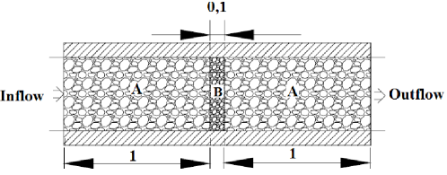
Fig. 1: Geometry of the domain

	Medium A	Medium B
Porosity $\phi$ ($-$)	0.25	0.5
Total immobile concentration $T_{S}$	1	10

Table 1: Physical properties of the materials

The chemical reactions are summarized in Table 3. The 7 reactions involve 9 mobile species (in the aqueous phase) and 3 immobile species (in the solid phase).

The characteristic feature of this chemical system is that it contains large stoichiometric coefficients that range from -4 to 4 and a large variation of equilibrium constants between $10^{-12}$ and $10^{35}$.

Boundary and initial conditions are presented in Table 3. The simulation involves an injection period followed by a leaching period, so that the system is returned to its initial state. Note that the total for the immobile species is given in Table 1.

	${X_{1}}$	${X_{2}}$	${X_{3}}$	${X_{4}}$	$S$	$K$
${C_{1}}$	0	-1	0	0	0	${\bf 10^{-12}}$
${C_{2}}$	0	1	1	0	0	1
${C_{3}}$	0	-1	0	1	0	1
${C_{4}}$	0	-4	1	$3$	0	$10^{-1}$
${C_{5}}$	0	${\bf 4}$	$3$	1	0	${\bf 10^{+35}}$
${CS_{1}}$	0	3	1	0	1	$10^{+6}$
${CS_{2}}$	0	-3	0	1	2	$10^{-1}$

Table 2: Morel tableau for Chemical equilibrium

Total	$T_{1}$	$T_{2}$	$T_{3}$	$T_{4}$
Conc.	0	-2	0	2
Injection	0.3	0.3	0.3	0
t$\in$[0,5000]
Leaching	0	-2	0	2
t$\in$[5000,..]

Table 3: Boundary conditions

6.1.1 Sample results

The results obtained in [11] indicate that one needs to refine the mesh around medium B if one is to obtain accurate results. For all test cases, we use a mesh such that $h_{A}=4h_{B}$. The computations were carried out with the various methods presented in this paper. When used with the appropriate numerical parameters they all gave comparable results. The figures in this section were obtained with the $h$-method.

Figure 2 shows profiles of the concentrations of several species. The left and middle images show concentrations of (a part of) mobile species $C1$ and immobile species $S$ at an early time $t=10$, whereas the right image shows concentration of aqueous species $C_{2}$ on a smaller interval during the leaching period, at $t=5010$. The middle image highlights the effect of the heterogeneity at $x=1$.

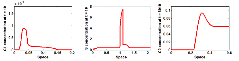
Fig. 2: Concentrations profiles. Left figure: $C_{1}$ at $t=10$, middle figure $S$ at $t=10$, right figure $C_{2}$ at $t=5010$.

Figure 3 shows elution curves, that is evolution of the concentrations at the end of the domain ($x=2.1$) as a function of time, for a mesh with $384$ elements. Notice that the evolution of $C5$ follows a fairly complex pattern. It turns out that the accuracy for both species $X3$ and $C5$ is quite sensitive to the mesh size used. We come back to this point in detail in the next subsection.

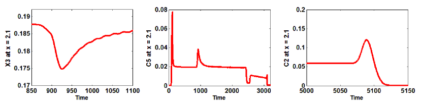
Fig. 3: Elution curves (concentrations at right end of the domain as a function of time). Left image: species $X3$, middle image: species $C5$, right image: species $C2$

The results shown on these figures are in good agreement with those showed by various groups in the comparison paper[11].

As mentioned above, some of the species show a very sensitive dependence on the mesh and time step used. It has proven necessary to use very fine meshes, as well as small time steps, in order to resolve these species accurately. We now study in more detail how the accuracy depends on the time and space meshes

6.1.2 Influence of spatial discretization

The evolution of species $X3$ and $C5$, as a function of time, exhibits unphysical oscillations. The origin of these oscillations has been explained in [41], and is due to the interplay between the very stiff reactions and the spatial discretizations. They should decrease as the mesh is refined.

Figures 4 shows that this is indeed what happens as we increase the number of discretization points. A mesh with 384 points gives qualitatively correct results, but we have also made use of a finer meshes in order to obtain more accurate results.

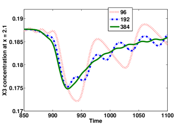
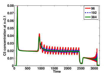
Fig. 4: Elution curves of $X_{3}$ (left) and $C_{5}$ (right) concentration, for various mesh resolutions

The effect of the mesh size on the accuracy of the results is also shown by looking in detail at two specific species: mobile species $C_{1}$ and immobile species $S$, both at time $t=10$. They both exhibit a sharp peak, and we focus on the accuracy with which the location and amplitude of the peak can be determined. These elements were part of the comparison criteria for the benchmark, and were examined in detail in [11].

We also discuss the influence of the discretization scheme, by comparing the three schemes introduced in section 3.2 from the point of view of accuracy. Their relative efficiencies are compared in section 6.1.4. In figures 5 and 6, the curves are labeled by the total number of discretization points in space. The coarsest mesh, corresponding to $n=96$, has $\Delta x=0.025$ in medium A and $\Delta x=0.00625$ in medium B. In both cases the time step was chosen as $\Delta t=\Delta t_{c}$ (advective time step), with a CFL=0.1, as given by the smaller space mesh in medium B. Note that since the CFL is fixed, each curve also corresponds to a different time step.

Figure 5 compares the concentrations of species $C_{1}$ on the interval $[0,0.2]$, at time $t=10$, as computed by the three discretization schemes on increasingly refined meshes. As soon as the mesh has sufficiently many points to successfully resolve the solution, all three schemes give identical solutions. On the other hand, one needs at least 384 points (and preferably 768) to obtain a satisfactory solution.

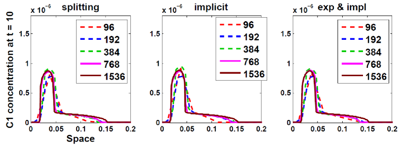
Fig. 5: Concentration of species $C_{1}$ at $t=10$ for the different discretization schemes and various mesh resolutions

Figure 6 compares the concentration of species $S$ (a sorbed species) on the interval bracketing the location of the peak $[0,0.15]$, at time $t=10$, as computed by the three discretization schemes on increasingly refined meshes. Here also, the three schemes give identical solutions when the mesh is fine enough. This time, one needs at least 768 mesh points to obtain a converged solution. One should compare Figure 6 in [11], and also refer to Table 4 there, where the location and amplitude of the peak are tabulated for all the methods used in the benchmark. We have obtained values of $x=0.0175$ for the location of the peak, and $S=0.985$ for its height. These values are in the range reported by the other teams, but are different form the “mean” values as reported in [11]. They are however very close to the “reference” values found in [10].

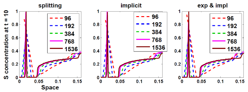
Fig. 6: Concentration of species $S$ at $t=10$ for the different discretization schemes and various mesh resolutions

6.1.3 Influence of temporal discretization

We now discuss the influence of the time step, or more precisely the value of the CFL coefficient (given by $CFL=u\phi\Delta t/h_{\min}$ on the accuracy.

The three schemes used for time discretization have different behavior with respect to the choice of time step:

The splitting method

allows the use of different time steps (and different numerical methods) for the advection and the diffusion step. The advection time step is restricted by the CFL condition (it is an explicit sub-step), whereas the time step for diffusion is not restricted by stability. We have used three different choices: chose the same time step for advection and diffusion (respecting the CFL condition), once with a CFL condition of 1, and once with a CFL condition of $0.1$, and choose a diffusion time step 3 times larger than the advection time step (the latter chosen by the CFL condition).

The fully implicit method

here there is only one time step, and no stability restriction. We have compared three time steps, corresponding to CFL coefficients of $0.1$, $1$ and $3$ respectively.

The explicit–implicit method

this method also imposes a single time step, and in addition it is subject to the stability condition of the explicit method, so the time step is restricted to $CFL\leq 1$. We compare 2 time steps, corresponding to CFL coefficients of $0.1$ and 1 respectively.

Figure 7 compares the concentration of species $S$ as computed by the three methods, for the time step sizes chosen as explained above, for two different mesh resolutions.

For all three methods the location of the peak was correctly determined even for larger values of the time step and the mesh size, but its amplitude was only correctly estimated for the finer mesh size.

For both splitting and explicit-implicit schemes, it is not necessary to use a CFL of 0.1 (a CFL of 1 is enough) for the peak amplitude to reach the value 1, but what is needed is to refine the mesh (up to 1536 nodes). However, the fully implicit scheme needs both a small time step corresponding to a CFL of 0.1 and a fine mesh with 1536 nodes to obtain the same results as the other schemes.

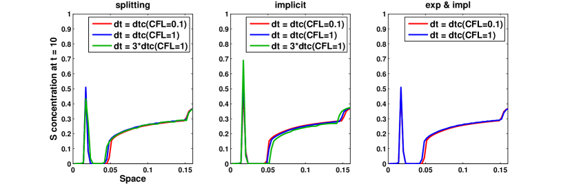
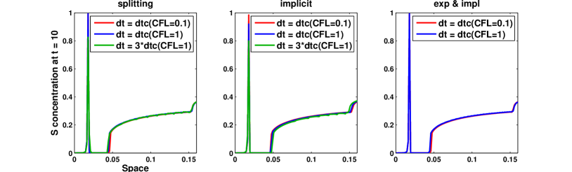
Fig. 7: Effect of the CFL condition on the concentrations in $S$ (top figure 768 nodes, bottom figure 1536 nodes)

6.1.4 CPU time

We now compare the relative efficiency of the three time discretization methods. One should keep in mind that the problem under study is a 1D model, so that solving a linear system is a not very time consuming. The conclusions reached below would have to be re-examined for a 2D (and even more for a 3D !) model. We have also compared the effect of using the fully implicit method with a variable time step (albeit not an adaptive choice, a sequence of pre-computed time steps is used for different phases of the solution evolution).

Figure 8 compares the CPU times required by the $h$-method with different time-discretization schemes as the space mesh is refined. The time step was chosen as follows (in all cases, the smallest mesh size was used):

For the splitting method

The diffusion time step is 3 times larger than the advection time step that respects a CFL coefficient of 1.

For the explicit-implicit method

One time step is used controlled by a CFL condition of 1.

For the fully implicit method

One time step is used corresponding to a CFL coefficient of 3 (no stability restriction).

For the fully implicit (variable) method

Variables time steps are used, as described in table 4. The time steps are chosen so as to have a small time step when strong variations happen due to the reactions (especially during injection and leaching period) and a large time step is used for the intervals that represent the steady state.

Start time	0	20	100	2500	3200	5000	5100
End time	20	100	2500	3200	5000	5100	6000
CFL value	1	5	10	5	40	1	40

Table 4: CFL values for variable time step simulation

As expected, using a variable time step results in large savings (while maintaining the accuracy). Among the 3 schemes with fixed time step, the explicit–implicit method is the most expensive, with the fully implicit and the splitting methods leading to comparable costs.

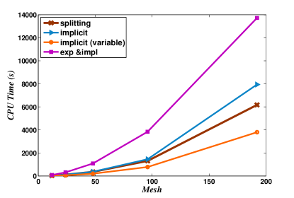
Fig. 8: CPU time required by the time discretization methods as the space mesh is refined

6.1.5 Influence of preconditioning strategy

In this section, we compare the various preconditioning strategies discussed in section 5. Our main criteria will be the number of linear and non-linear iterations. We have not tried to optimize the inexact Newton strategy, but have just relied on the default choices as provided in the Newton–Krylov code (we use the nsoli code from the book by C. T. Kelley [35]). In all experiments, GMRES was used without restart, and with a maximum number of allowed iterations fixed at 40.

Figure 9 shows how these numbers change as the mesh is refined. The various linear preconditioning strategies (applied to the coupled system) are compared with the elimination, or nonlinear preconditioning, strategy. As predicted, the nonlinear elimination strategy has the smallest number both for non-linear and for linear iterations. It also shows a behavior that is independent of the mesh size.

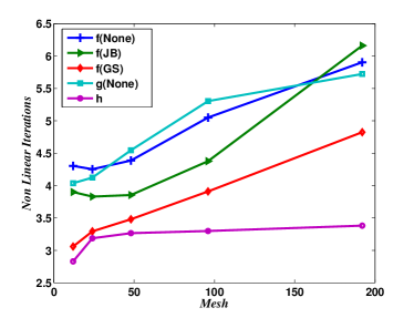
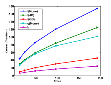
Fig. 9: Non-linear (left) and linear (right) iterations for different preconditioning strategies

The unpreconditioned method is unsurprisingly non scalable, at least as far as the linear iterations are concerned. The number of non-linear iterations grows only weakly with the number of mesh points. The same is true for Jacobi preconditioning.

Gauss–Seidel preconditioning, on the other hand, show only a modest increase in the number of linear iterations, and a behavior for the non-linear iterations that is in between that of the unpreconditioned and the elimination strategies.

As explained in section 5, a limitation of the elimination strategy is that it requires an exact solution of the transport step. In this case, the Gauss–Seidel preconditioner might prove useful: replacing the transport solve step by an approximation, such as several iterations of a multi-grid solver, should lead to a more efficient solution method, with similar convergence behavior. We plan to explore this strategy in a forthcoming work.

Last, figure 10 shows the time required by the various methods. Since the cost of the methods is comparable, the ordering is the same as that in the previous figure. It confirms the good efficiency of the elimination strategy, with Gauss–Seidel preconditioning as a distant second.

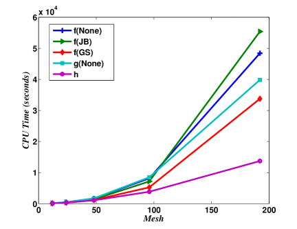
Fig. 10: CPU time as a function of the mesh size for the various solution methods

We can try and summarize the relative performances of the various methods as follows:

• the original $f$ formulation is not numerically scalable, neither at the non-linear level, nor at the linear level;

• the block Jacobi preconditioner applied to $f$ does not bring any improvement;

• the block Gauss–Seidel preconditioner improves the linear performance, but does have a significant non-linear effect (nor was it expected);

• the $g$ formulation improves the linear performance, but not as much as Gauss–Seidel preconditioning;

• the $h$ formulation, after elimination of the $C$ unknowns is the only method that gives a convergence independent of the mesh size.

Of course, these conclusions are more or less natural: methods $f$ and $g$ keep the ill-conditioning from the second order operator (except for $g$ at the linear level). The elimination method, leads to a bounded operator on $L^{2}$ (at least formally), and is expected to give mesh independent convergence.

This good performance of the elimination method, at least on the linear level, can be confirmed by looking at the field of values of the matrix $J_{h}$. The field of values of a matrix is the subset of the complex plane defined by

$$W(J_{h})=\left\{\dfrac{x^{H}J_{h}x}{x^{H}x},x\in\mathbf{C},x\neq 0\right\}.$$

It includes the eigenvalues and is a convex set. For a non-symmetric matrix, the convergence of GMRES is better described by the field of values than by the eigenvalues (see [6] or [37]). We conjecture that the field of values of the Schur complement $J_{h}$ can be bounded away from 0, independently of $N_{x}$. Though we have no proof at the moment, we have the following numerical confirmation on figure 11, which shows the field of values and isolines of the $\epsilon$-pseudo-spectra of the Jacobian matrix $J_{h}$ for 2 different mesh sizes. One can see that the convex hull of the field of values is indeed approximately independent of the mesh size. The figure was obtained thanks to the Eigtool software [70, 71].

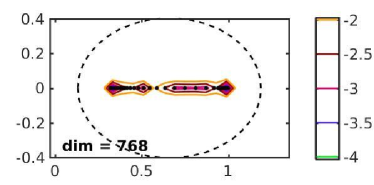
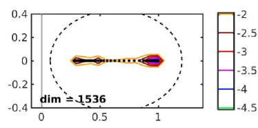
Fig. 11: Field of values (dashed line) and pseudo-spectra (color) for matrix $J_{h}$, with $N_{x}=768$ and $N_{x}=1536$

6.2 Test 2. Ions exchange in a natural system

Our second test case comes for a field study that includes experimental results (see Valocchi et al [68]). We follow the setup given in Fahs et al [24], as this reference includes more details for the numerical simulation. In this test case, four aqueous components ($\text{Na}^{+}$, $\text{Ca}^{2+}$, $\text{Mg}^{2+}$ and $\text{Cl}^{-}$) are injected into an homogeneous landfill. During the transport, the aqueous components react with the ion exchange sites of the soil (S). Three reactions of ion exchange occur and lead to three adsorbed species S–Na, S2–Ca, S2–Mg.
Chemical reactions, constants of equilibrium, initial and boundary conditions are summarized in Table  5.

	$\text{Na}^{+}$	$\text{Ca}^{2+}$	$\text{Mg}^{2+}$	$\text{Cl}^{-}$	S	log K
S–Na	1	0	0	0	1	4
S2–Ca	0	1	0	0	2	8.602
S2–Mg	0	0	1	0	2	8.355
initial (mmol/l)	248	165	168	161	750
injected (mmol/l)	9.4	2.12	0.494	9.03

Table 5: Chemical reactions, initial and boundary conditions

In this test, we consider a column of length L=16 m. The values of the transport parameters are given in Table  6

Darcy velocity	u=0.2525 [m/h]
Dispersion coefficient	D=0.74235 [m2/h]
Porosity	0.35

Table 6: Transport parameters

The simulated time is T=5000 h. The mesh size is equal to 0.08m , the time step is equal to 0.11089 h corresponding to CFL coefficients of 1.

Figure 12 shows the evolution of the concentrations in $\text{Ca}^{2+}$ and $\text{Mg}^{2+}$ at the end of the column, as a function of time (we use the same units as Fahs et al [24] which are different than those originally used by Valocchi et al [68]).

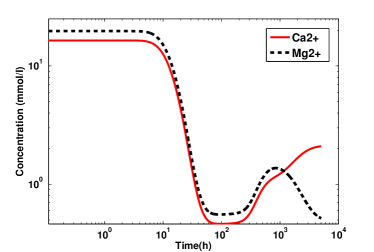
Fig. 12: Variation of $\text{Ca}^{2+}$ and $\text{Mg}^{2+}$ concentrations as function of time in the output of the domain

The results are in qualitative agreement with those in both references (Figure 1 in Fahs et al [24], Figure 11 in Valocchi et al [68]), though it appears difficult to make a precise comparison as the curves are in logarithmic scale on both axes.

Finally, figure 13 compares the number of linear and non-linear iterations for the various methods presented. In this case, the number of non-linear iterations was very close for all methods (with Block-Jacobi preconditioning a close winner), and both the Gauss-Seidel preconditioning and the $h$-method again giving a convergence independent of the mesh size

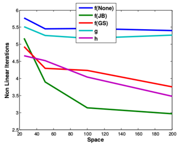
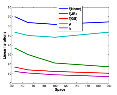
Fig. 13: Number of non-linear (left) and linear (right) iterations for ion exchange example

7 Conclusion and perspectives

In this work, several methods for improving the efficiency of a global approach for coupling transport and chemistry based on a Newton-Krylov method were studied.

An alternative formulation and block preconditioners for linear system were used to accelerate the convergence of the Krylov method and to reduce CPU time. The results show that the alternative formulation requires less CPU time than other preconditioners, and the number of linear and non linear iterations becomes almost independent of the mesh.

The reactive transport benchmark 1D problem proposed by GNR MoMaS was used to demonstrate the efficiency of the method.

Natural extensions of this work to multidimensional situations are under way, as well as extensions to handle kinetic reactions.

References

- [1] E. Ahusborde, M. Kern, and V. Vostrikov, Numerical simulation of two-phase multicomponent flow with reactive transport in porous media: application to geological sequestration of CO2, ESAIM: Proc., 50 (2015), pp. 21–39.
- [2] L. Amir and M. Kern, A global method for coupling transport with chemistry in heterogeneous porous media, Computat. Geosci., 14 (2010), pp. 465–481. 10.1007/s10596-009-9162-x.
- [3] C. A. J. Appelo and D. Postma, Geochemistry, Groundwater and Pollution, CRC Press, 2nd ed., 2005.
- [4] P. Audigane, I. Gaus, I. Czernichowski-Lauriol, K. Pruess, and T. Xu, Two-Dimensional reactive transport modeling of CO2 injection in a saline aquifer at the Sleipner site, North sea, American journal of science, 307 (2007), pp. 974–1008.
- [5] J. Bear and A. H.-D. Cheng, Modeling Groundwater Flow and Contaminant Transport, vol. 23 of Theory and Applications of Transport in Porous Media, Springer, 2010.
- [6] M. Benzi and M. A. Olshanskii, Field-of-values convergence analysis of augmented Lagrangian preconditioners for the linearized Navier–Stokes problem, SIAM J. Numer. Anal., 49 (2011), pp. 770–788.
- [7] C. M. Bethke, Geochemical and Biogeochemical Reaction Modeling, Cambridge University Press, 2nd ed., 2008.
- [8] Å. Björck, Numerical methods for least squares problems, Society for Industrial and Applied Mathematics, Philadelphie, 1996.
- [9] X.-C. Cai and D. E. Keyes, Nonlinearly preconditioned inexact Newton algorithms, SIAM J. Sci. Comput., 24 (2002), pp. 183–200.
- [10] J. Carrayrou, Looking for some reference solutions for the reactive transport benchmark of MoMaS with SPECY, Computat. Geosci., 14 (2010), pp. 393–403.
- [11] J. Carrayrou, J. Hoffmann, P. Knabner, S. Kräutle, C. de Dieuleveult, J. Erhel, J. van der Lee, V. Lagneau, K. U. Mayer, and K. T. B. MacQuarrie, Comparison of numerical methods for simulating strongly nonlinear and heterogeneous reactive transport problems-the MoMaS benchmark case, Computat. Geosci., 14 (2010), pp. 483–502.
- [12] J. Carrayrou, M. Kern, and P. Knabner, Reactive transport benchmark of MoMaS, Computat. Geosci., 14 (2010), pp. 385–392. 10.1007/s10596-009-9157-7.
- [13] J. Carrayrou, R. Mosé, and P. Behra, New efficient algorithm for solving thermodynamic chemistry, Aiche J., 48 (2002), pp. 894–904.
- [14] J. Carrayrou, R. Mosé, and P. Behra, Operator-splitting procedures for reactive transport and comparison of mass balance errors, J. Contam. Hydrol., 68 (2004), pp. 239–268.
- [15] A. Chilakapati, T. Ginn, and J. Szecsody, An analysis of complex reaction networks in groundwater modeling, Water Resour. Res., 34 (1998), pp. 1767–1780.
- [16] C. de Dieuleveult and J. Erhel, A global approach to reactive transport: application to the MoMas benchmark, Computat. Geosci., 14 (2010), pp. 451–464.
- [17] C. de Dieuleveult, J. Erhel, and M. Kern, A global strategy for solving reactive transport equations, J. Comput. Phys., 228 (2009), pp. 6395–6410.
- [18] L. De Windt, D. Pellegrini, and J. van der Lee, Coupled modeling of cement/claystone interactions and radionuclides migration, J. Contam. Hydrol., 68 (2004), pp. 165–182.
- [19] P. Deuflhard, Newton Methods for Nonlinear Problems. Affine Invariance and Adaptive Algorithms, vol. 35 of Springer Series in Computational Mathematics, Springer, 2011.
- [20] J. Erhel and T. Migot, Characterizations of Solutions in Geochemistry: Existence, Uniqueness and Precipitation Diagram. working paper or preprint, Sept. 2017.
- [21] J. Erhel and S. Sabit, Analysis of a global reactive transport model and results for the momas benchmark, Math. Comput. Simul., 137 (2017), pp. 286–298.
- [22] J. Erhel, S. Sabit, and C. de Dieuleveult, Solving partial differential algebraic equations and reactive transport models, in Developments in Parallel, Distributed, Grid and Cloud Computing for Engineering, B. H. V. Topping and P. Ivànyi, eds., Computational Science, Engineering and Technology Series, Saxe Coburg Publications, 2013, pp. 151–169.
- [23] R. Eymard, T. Gallouët, and R. Herbin, Finite volume methods, in Handbook of Numerical Analysis, P. G. Ciarlet and J. L. Lions, eds., vol. VII, North–Holland, 2000, pp. 713–1020.
- [24] M. Fahs, J. Carrayrou, A. Younes, and P. Ackerer, On the efficiency of the direct substitution approach for reactive transport problems in porous media, Water, Air, and Soil Pollution, 193 (2008), pp. 299–308.
- [25] Y. Fan, L. J. Durlofsky, and H. A. Tchelepi, A fully-coupled flow-reactive-transport formulation based on element conservation, with application to CO 2 storage simulations, Adv. Water Resour., 42 (2012), pp. 47–61.
- [26] G. H. Golub and C. F. van Loan, Matrix Computations, Johns Hopkins University Press, 4th ed., 2013.
- [27] G. E. Hammond, P. C. Lichtner, and R. T. Mills, Evaluating the performance of parallel subsurface simulators: An illustrative example with PFLOTRAN, Water Resources Research, 50 (2014), pp. 208–228.
- [28] G. E. Hammond, A. Valocchi, and P. Lichtner, Application of Jacobian-free Newton–Krylov with physics-based preconditioning to biogeochemical transport, Adv. Water Resour., 28 (2005), pp. 359–376.
- [29] J. Hoffmann, S. Kräutle, and P. Knabner, A parallel global-implicit 2-D solver for reactive transport problems in porous media based on a reduction scheme and its application to the momas benchmark problem, Comput Geosci, 14 (2009), pp. 421–433.
- [30] H. Hoteit, P. Ackerer, and R. Mosé, Nuclear waste disposal simulations: Couplex test cases: Simulation of transport around a nuclear waste disposal site: The COUPLEX test cases (editors: Alain Bourgeat and Michel Kern), Computat. Geosci., 8 (2004), pp. 99–124.
- [31] V. E. Howle, R. C. Kirby, and G. Dillon, Block preconditioners for coupled physics problems, SIAM J. Sci. Comput., 35 (2013), pp. S368–S385.
- [32] I. C. F. Ipsen, A note on preconditioning nonsymmetric matrices, SIAM J. Sci. Comput., 23 (2001), pp. 1050–1051.
- [33] D. Jara Heredia, J.-R. de Dreuzy, and B. Cochepin, TReacLab: an object oriented implementation of non intrusive operator splitting methods to couple independent transport and geochemical software, Comput. Geosci., (2017). to appear.
- [34] C. T. Kelley, Iterative methods for linear and nonlinear equations, vol. 16 of Frontiers in Applied Mathematics, SIAM, Philadelphia, PA, 1995. With separately available software.
- [35] , Solving Nonlinear Equations with Newton’s Method, vol. 1 of Fundamentals of Algorithms, SIAM, Philadelphia, PA, 2003. With separately available software.
- [36] M. Kern and A. Taakili, Linear and nonlinear preconditioning for reactive transport, in XVIII Conference on Computational Methods in Water Resources CMWR XVIII, J. Carrera, P. Binning, and G. F. Pinder, eds., 2010. https://hal.inria.fr/inria-00581566/document.
- [37] A. Klawonn and G. Starke, Block triangular preconditioners for nonsymmetric saddle point problems: field-of-values analysis, Numer. Math., 81 (1999), pp. 577–594.
- [38] D. A. Knoll and D. E. Keyes, Jacobian-free Newton-Krylov methods: a survey of approaches and applications, J. Comput. Phys., 193 (2004), pp. 357–397.
- [39] S. Kräutle and P. Knabner, A new numerical reduction scheme for fully coupled multicomponent transport-reaction problems in porous media, Water Resour. Res., 41 (2005).
- [40] , A reduction scheme for coupled multicomponent transport-reaction problems in porous media: Generalization to problems with heterogeneous equilibrium reactions, Water Resour. Res., 43 (2007).
- [41] V. Lagneau and J. van der Lee, HYTEC results of the MoMas reactive transport benchmark, Computat. Geosci., 14 (2010), pp. 435–449.
- [42] H. Machat and J. Carrayrou, Comparison of linear solvers for equilibrium geochemistry computations, Computational Geosciences, 21 (2017), pp. 131–150.
- [43] K. T. B. MacQuarrie and K. U. Mayer, Reactive transport modeling in fractured rock: A state-of-the-science review, Earth Science Reviews, 72 (2005), pp. 189–227.
- [44] M. Marinoni, J. Carrayrou, Y. Lucas, and P. Ackerer, Thermodynamic equilibrium solutions through a modified Newton Raphson method, AIChE Journal, 63 (2017), pp. 1246–1262.
- [45] N. C. Marty, C. Tournassat, A. Burnol, E. Giffaut, and E. C. Gaucher, Influence of reaction kinetics and mesh refinement on the numerical modelling of concrete/clay interactions, Journal of Hydrology, 364 (2009), pp. 58–72.
- [46] N. C. M. Marty, O. Bildstein, P. Blanc, F. Claret, B. Cochepin, E. C. Gaucher, D. Jacques, J.-E. Lartigue, S. Liu, K. U. Mayer, J. C. L. Meeussen, I. Munier, I. Pointeau, D. Su, and C. I. Steefel, Benchmarks for multicomponent reactive transport across a cement/clay interface, Computat. Geosci., 19 (2015), pp. 635–653.
- [47] P. Marzal, A. Seco, J. Ferrer, and C. Gabalón, Modeling multiple reactive solute transport with adsorption under equilibrium and nonequilibrium conditions, Adv. Water Resour., 17 (1994), pp. 363–374.
- [48] K. U. Mayer, E. O. Frind, and D. W. Blowes, Multicomponent reactive transport modeling in variably saturated porous media using a generalized formulation for kinetically controlled reactions, Water Resour. Res., 38 (2002), pp. 13–1–13–21. 1174.
- [49] C. D. Meyer, Matrix Analysis and Applied Linear Algebra, SIAM, 2000.
- [50] F. M. M. Morel and J. G. Hering, Principles and Applications of Aquatic Chemistry, Wiley, New-York, 1993.
- [51] M. F. Murphy, G. H. Golub, and A. J. Wathen, A note on preconditioning for indefinite linear systems, SIAM J. Sci. Comput., 21 (2000), pp. 1969–1972.
- [52] J. Rubin, Transport of reacting solutes in porous media: Relation between mathematical nature of problem formulation and chemical nature of reactions, Water Resour. Res., 19 (1983), pp. 1231–1252.
- [53] Y. Saad and M. H. Schultz, GMRES: a generalized minimal residual algorithm for solving nonsymmetric linear systems, SIAM J. Sci. Statist. Comput., 7 (1986), pp. 856–869.
- [54] M. Saaltink, C. Ayora, and J.Carrera, A mathematical formulation for reactive transport that eliminates mineral concentrations, Water Resour. Res., 34 (1998), pp. 1649–1656.
- [55] M. Saaltink, J. Carrera, and C. Ayora, A comparison of two approaches for reactive transport modelling, Journal of Geochemical Exploration, 69-70 (2000), pp. 97–101.
- [56] M. Saaltink, J. Carrera, and C. Ayora, On the behavior of approaches to simulate reactive transport, J. Contam. Hydrol., 48 (2001), pp. 213–235.
- [57] M. Saaltink, V. Vilarrasa, F. De Gaspari, O. Silva, J. Carrera, and T. Roetting, A method for incorporating equilibrium chemical reactions into multiphase flow models for CO2 storage, Adv. Water resour., 62 (2013), pp. 431–441.
- [58] J. Samper, H. Ma, J. L. Cormenzana, C. Lu, L. Montenegro, and M. . A. Cuñado, Testing Kd models of Cs+ in the near field of a HLW repository in granite with a reactive transport model, Physics and Chemistry of the Earth, Parts A/B/C, 35 (2010), pp. 278–283.
- [59] J. Samper, T. Xu, and C. Yang, A sequential partly iterative approach for multicomponent reactive transport with CORE2D, Computat. Geosci., 13 (2008), pp. 301–316.
- [60] P. Siegel, R. Mosé, P. Ackerer, and J. Jaffré, Solution of the advection-dispersion equation using a combination of discontinuous and mixed finite elements, Int. J. Numer. Meth. Fl., 24 (1997), pp. 595–613.
- [61] I. Sin, V. Lagneau, and J. Corvisier, Integrating a compressible multicomponent two-phase flow into an existing reactive transport simulator, Adv, Water Resour., 100 (2017), pp. 62–77.
- [62] B. Southworth, T. Manteuffel, S. McCormick, S. Munzenmaier, and J. Ruge, Reduction-based Algebraic Multigrid for Upwind Discretizations, ArXiv e-prints, (2017).
- [63] C. Steefel, D. DePaolo, and P. Lichtner, Reactive transport modeling: An essential tool and a new research approach for the earth sciences, Earth and Planetary Science Letters, 240 (2005), pp. 539–558.
- [64] C. I. Steefel, C. A. J. Appelo, B. Arora, D. Jacques, T. Kalbacher, O. Kolditz, V. Lagneau, P. C. Lichtner, K. U. Mayer, J. C. L. Meeussen, S. Molins, D. Moulton, H. Shao, J. S̃imůnek, N. Spycher, S. B. Yabusaki, and G. T. Yeh, Reactive transport codes for subsurface environmental simulation, Computat. Geosci., 19 (2015), pp. 445–478.
- [65] G. Strang, Introduction to Linear Algebra, Wellesley-Cambridge Press, 4th ed., 2009.
- [66] L. Trenty, A. Michel, E. Tillier, and Y. L. Gallo, A sequential splitting strategy for CO2 storage modelling, in ECMOR X - 10th European Conference on the Mathematics of Oil Recovery, EAGE, 2006.
- [67] A. J. Valocchi and M. Malmstead, Accuracy of operator splitting for advection-dispersion-reaction problems, Water Resour. Res., 28 (1992), pp. 1471–1476.
- [68] A. J. Valocchi, R. L. Street, and P. V. Roberts, Transport of ion-exchanging solutes in groundwater: Chromatographic theory and field simulation, Water Resources Research, 17 (1981), pp. 1517–1527.
- [69] J. A. White and R. I. Borja, Block-preconditioned Newton–Krylov solvers for fully coupled flow and geomechanics, Computat. Geosci., 15 (2011), pp. 647–659.
- [70] T. G. Wright, Eigtool. http://www.comlab.ox.ac.uk/pseudospectra/eigtool/, 2002.
- [71] T. G. Wright and L. N. Trefethen, Large-scale computation of pseudospectra using ARPACK and Eigs, SIAM J. Sci. Comput., 23 (2001), pp. 591–605.
- [72] G. T. Yeh and V. S. Tripathi, A critical evaluation of recent developments in hydrogeochemical transport models of reactive multichemical components, Water Resour. Res., 25 (1989), pp. 93–108.
- [73] G.-T. Yeh and V. S. Tripathi, A model for simulating transport of reactive multispecies components: Model development and demonstration, Water Resour. Res., 27 (1991), pp. 3075–3094.
- [74] F. Zhang, G. Yeh, and J. Parker, eds., Groundwater Reactive Transport Models, Bentham Publishers, 2012.