Multi-scale Invariant Fields: Estimation and Prediction

Abstract

Extending the concept of multi-selfsimilar random field we study multi-scale invariant (MSI) fields which have component-wise discrete scale invariant property. Assuming scale parameters as $\lambda_{i}>1$, $i=1,\ldots,d$ and the parameter space as $(1,\infty)^{d}$, the first scale rectangle is referred to the rectangle $(1,\lambda_{1})\times\ldots\times(1,\lambda_{d})$. We show that the covariance function of the sampled Markov MSI field are characterized by the variances and covariances of samples inside first scale rectangle. As an example of MSI field, a two-dimensional simple fractional Brownian sheet (sfBs) is demonstrated. Also real data of the precipitation in some area of Brisbane in Australia for two days (25 and 26 January 2013) are examined. We show that precipitation on this area has MSI property and estimate it as a simple MSI field with stationary increments inside scale intervals. This structure enables us to predict the precipitation in surface and time. We apply the mean absolute percentage error as a measure for the accuracy of the predictions.


Mathematics Subject Classification MSC 2010: 60G18; 60G22; 62M15; 62H05.

Keywords: Scale invariant Random fields; Self-similarity; Modeling Precipitation, Estimation and Forecasting.

1 Introduction

Gaussian self-similar fields have been extensively studied and applied in various area as hydrology, biology, economics, finance and image processing [31]. In probability theory, a random field is a family of random variables indexed in a multi-dimensional space.
As stated by Genton et al. [15], a random field $\{X(\mathbf{t}),\mathbf{t}\in\mathbb{R}^{d}\}$ is said to be multi-selfsimilar (MSS) if for some Hurst vector $\mathbf{H}=(H_{1},\cdots,H_{d})>{\bf 0}$ and any $\boldsymbol{\Lambda}=(\lambda_{1},\cdots,\lambda_{d})>{\bf 1}$

$${\bf X}({\bf\Lambda}\circ{\bf t})\overset{\mathcal{L}}{=}\big{(}\prod_{i=1}^{d}\lambda_{i}^{H_{i}}\big{)}{\bf X(t)}.$$ (1.1)

where $\mathbf{H}=(H_{1},\ldots,H_{d})$, $\boldsymbol{\Lambda}=(\lambda_{1},\ldots,\lambda_{d})$ and $\overset{\mathcal{L}}{=}$ denotes equality of finite dimensional distributions, and $\circ$ is the Hadamard product that operates as $\boldsymbol{\Lambda}\circ\mathbf{t}=(\lambda_{1}t_{1},\ldots,\lambda_{d}t_{d})$. The random field is said to be multi-scale invariant (MSI) of index $\mathbf{H}$ and scale $\boldsymbol{\Lambda}^{\prime}=(\lambda^{\prime}_{1},\ldots,\lambda^{\prime}_{d})$, if (1.1) holds for some case $\boldsymbol{\Lambda}=\boldsymbol{\Lambda}^{\prime}$. In one-dimensional, the discrete scale invariant (DSI) process initially studied by Borgnat et al. [8] is a scale invariance or self-similar process only for specific choice of scale parameter. Balasis et al [4, 5, 6] and Bartolozzi et al [7] have studied wide range of applications of DSI processes in Dynamic Magnetosphere, DST time series and stock markets.

Let $\{X(\mathbf{t}),\mathbf{t}\in[1,\infty)^{d}\}$ be some MSI field with prescribed scale vector $\boldsymbol{\Lambda}=(\lambda_{1},\ldots,\lambda_{d})$ where $\lambda_{i}$’s are greater than one. Extending the method of Modarresi and Rezakhah [21, 22], we consider component-wise geometric sampling of the field at points $\boldsymbol{\alpha}^{\mathbf{k}}=(\alpha_{1}^{k_{1}},\ldots,\alpha_{d}^{k_{d}})^{T}$, $k_{1},k_{2},\ldots,k_{d}\in\mathbb{N}_{0}=\{0,1,\ldots\}$, to get $\{X(\boldsymbol{\alpha}^{\mathbf{k}}),\boldsymbol{\alpha}^{\mathbf{k}}\in{\mathbb{R}}^{d}\}$ as the sampled MSI field, where $\alpha_{i}$’s are determined by $\lambda_{i}=\alpha_{i}^{n_{i}}$ for $i=1,2,\ldots,d$ while $n_{1},\ldots,n_{d}$ are arbitrary positive integers. So we have $\prod_{i=1}^{d}n_{i}$ observations in the first scale rectangle $[1,\lambda_{1})\times\ldots\times[1,\lambda_{d})$. In general we consider d-dimensional $(k_{1},k_{2},\ldots,k_{d})$ scale rectangle as

$$[\lambda_{1}^{k_{1}-1},\lambda_{1}^{k_{1}})\times[\lambda_{2}^{k_{2}-1},\lambda_{2}^{k_{2}})\times\ldots\times[\lambda_{d}^{k_{d}-1},\lambda_{d}^{k_{d}}).$$ (1.2)

The first scale rectangle is considered as the d-dimensional $(1,1,\ldots,1)$ scale rectangle. The MSI field with Markov property is called Markov MSI (MMSI). We show that the covariance function of the sampled MMSI field are presented by the covariance function of corresponding samples inside the first scale rectangles. We present some proper estimation method based on this component-wise sampling scheme by extending the method of estimation the parameters for DSI processes in [27, 28].
This paper is motivated by applications in environmental and climate phenomena. Precipitation is one of the key terms for balancing the energy budget, and one of the most challenging aspects of climate modeling. Basic research performed in the statistical analysis and studied the variability in the distribution of rainfall to obtain accurate prediction [26], [33]. As an example of MSI field, real data of the precipitation in some part of Brisbane area of Australia for some special period of time are considered. The MSI behavior of these precipitation in three dimension as latitude, longitude and time are verified [13]. Also the corresponding time dependent scale and Hurst parameter of the MSI field are estimated. By estimating these parameters, we predict the precipitation in surface and time. All prediction methods have errors in predicting. So we use mean absolute percentage error (MAPE) as a statistical measure that calculate the error of the predictions. We show that our predictions are highly accurate.

The rest of the paper is organized as follows. Section 2 is devoted to some preliminaries and also definitions of MSS and MSI fields. The component-wise geometric sampling scheme and some proper quasi-Lamperti transformation are defined in this section. The definition of a two-dimensional simple fractional Brownian sheet (sfBs) as an example of MSI field is given in section 2 as well. The characterization of covariance and spectral density functions of the two-dimensional scale invariant wide-sense Markov fields are presented in section 3. In section 4 we introduce a heuristic method for the estimation of Hurst parameter of MSI fields. Implying the rainfall data of Brisbane area of Australian bureau of meteorology, their MSI property of the field is verified and also the scale and Hurst parameters of this field are estimated. Finally, we study the prediction of the precipitation and employ the mean absolute percentage error(MAPE) index to determine the accuracy of the prediction.

2 Theoretical Structure

In this section, we present the definitions of the multi-selfsimilar (MSS) and multi-scale invariant (MSI) fields to be prescribed by some parameter space. Then we introduce a modified version of Lamperti transformation which provides a one to one correspondence between sampled MSS and discrete time stationary fields and also between sampled MSI and discrete time periodic fields respectively.
First we present the definition of periodic field and we use them as the Lamperti counterpart of self-similar field to obtain the covariance structure of MSI field.

Definition 1.

The random field is said to be stationary field if for any $\tau\in\mathbb{R}^{d}$

$$\{\mathcal{S}_{\boldsymbol{\tau}}X(\mathbf{t}),t\in\mathbb{R}^{d}\}\overset{\mathcal{L}}{=}\{X(\mathbf{t}),t\in\mathbb{R}^{d}\},$$

where for any $t$ and $\boldsymbol{\tau}\in\mathbb{R}^{d}$, the shift operator $\mathcal{S}_{\boldsymbol{\tau}}$ acts as $\mathcal{S}_{\boldsymbol{\tau}}X(\mathbf{t}):=X(\mathbf{t}+{\boldsymbol{\tau}}).$ The random field is called periodic with period $\boldsymbol{\tau}_{0}$ if the above equality holds just for $\boldsymbol{\tau}=\boldsymbol{\tau}_{0}$.

Definition 2.

A second order random field is called periodically correlated (PC) if its mean and covariance function has a periodic structure for some $\boldsymbol{\tau}$, see [18]

$$E[X(\mathbf{t}+\boldsymbol{\tau})]=E[X(\mathbf{t})],\hskip 72.26999ptCov(X(\mathbf{t}),X(\mathbf{s}))=Cov(X(\mathbf{t}+\boldsymbol{\tau}),X(\mathbf{s}+\boldsymbol{\tau})).$$

Periodic field with finite second moment is also a PC random field.

It should be noted that a second order random field is square integrable over the parameter space. Extending some definitions in Modarresi et al. [21] for DSI process with some parameter space, we present the following definitions.

Definition 3.

A random field $\{X(\mathbf{k}),\mathbf{k}\in\check{\mathbf{T}}\}$ is called MSS with parameter space $\check{\mathbf{T}}$, where $\check{\mathbf{T}}$ is any subset of $[1,\infty)^{d}$ and for any $\mathbf{k}_{1}=(k_{11},k_{12},\ldots,k_{1d})^{T}$, $\mathbf{k}_{2}=(k_{21},k_{22},\ldots,k_{2d})^{T}\in\check{\mathbf{T}}$

$$\{X(\mathbf{k}_{2})\}\overset{\mathcal{L}}{=}\Big{(}\prod_{i=1}^{d}\big{(}\frac{k_{2i}}{k_{1i}}\big{)}^{H_{i}}\Big{)}\{X(\mathbf{k}_{1})\}.$$ (2.1)

The random field $X(\cdot)$ is called MSI with parameter space $\check{\mathbf{T}}$ and scale $\boldsymbol{\Lambda}=(\lambda_{1},\ldots,\lambda_{d})$ if for any $\mathbf{k}_{1},\mathbf{k}_{2}\in\check{\mathbf{T}}$, (2.1) holds where $k_{2i}=\lambda_{i}k_{1i}$ and $\lambda_{i}>1$ for $i=1,\ldots,d$. Furthermore, it is to mention that the Hurst parameter in these fields are not restricted with one and might be some other finite values.

Now, we are to consider some geometric sampling of the MSI field at points $\boldsymbol{\alpha}=(\alpha_{1},\ldots,\alpha_{d})^{T}$ where $\alpha_{i}>1$ for $i=1,\ldots,d$.

Remark 1.

By assuming $k_{1},\ldots,k_{d}$ to be fixed integers $k_{i}\in\{1,2,\ldots,n_{i}\}$ and sampling of the MSI field at points $\big{\{}\boldsymbol{\alpha}^{\mathbf{l}\mathbf{n}+\mathbf{k}}=(\alpha_{1}^{l_{1}n_{1}+k_{1}},\ldots,\alpha_{d}^{l_{d}n_{d}+k_{d}})^{T}:l_{i}\in\mathbb{N}_{0},i=1,\ldots,d\big{\}}$ we have an MSS field with parameter space $\check{\mathbf{T}}=\{\boldsymbol{\alpha}^{\mathbf{l}\mathbf{n}+\mathbf{k}},\mathbf{l}\in\mathbb{N}_{0}^{d}\}$.

Similar to the concept of the wide-sense self-similar process presented by Nuzman et al. [25], we have the following definition.

Definition 4.

A second order random field $\{X(\mathbf{t}),\mathbf{t}\in\mathbb{R}^{d}_{+}\}$ is said to be wide-sense MSS with index $\mathbf{H}=(H_{1},\ldots,H_{d})$, if the following properties are satisfied for ${\mathbf{t},\mathbf{t}_{1},\mathbf{t}_{2}}\in\mathbb{R}^{d}_{+}$ and $\mathbf{a}=(a_{1},\ldots,a_{d})$ where $a_{i}>0$
          $(i)E[X^{2}(\mathbf{t})]<\infty$
$(ii)E[X(\mathbf{a\circ t})]=\big{(}\prod_{i=1}^{d}a_{i}^{H_{i}}\big{)}E[X(\mathbf{t})]$
$(iii)E[X(\mathbf{a\circ t_{1}})X(\mathbf{a\circ t_{2}})]=\big{(}\prod_{i=1}^{d}a_{i}^{2H_{i}}\big{)}E[X(\mathbf{t_{1}})X(\mathbf{t_{2}})]$
where $\circ$ is the Hadamard product defined in (1.1). This field is called wide-sense MSI of index $\mathbf{H}$ and scale $\mathbf{a}^{\prime}=(a^{\prime}_{1},\ldots,a^{\prime}_{d})$ where $a^{\prime}_{i}>0$, if the above conditions hold for some $\mathbf{a}=\mathbf{a}^{\prime}$.

To find a one-to-one correspondence between the shift and renormalized operators and also between MSI and periodic fields, we introduce the quasi-Lamperti transformation. In the rest of the paper we consider MSS and MSI in the wide-sense fields, so for simplicity we omit the term ”in the wide sense” henceforth.

Definition 5.

The quasi-Lamperti transform $\mathcal{L}_{\mathbf{H},\boldsymbol{\alpha}}$ with positive Hurst vector $\mathbf{H}=(H_{1},\ldots,H_{d})$ and positive scale vector $\boldsymbol{\alpha}=(\alpha_{1},\ldots,\alpha_{d})$, operates on a random field $\{Y(\mathbf{t}),\mathbf{t}\in\mathbb{R}^{d}_{+}\}$ as

$$\mathcal{L}_{\mathbf{H},\boldsymbol{\alpha}}Y(\mathbf{t})=\big{(}\prod_{i=1}^{d}t_{i}^{H_{i}}\big{)}Y(\mathbf{Log}_{\boldsymbol{\alpha}}\mathbf{t}),$$ (2.2)

where $\mathbf{Log}_{\boldsymbol{\alpha}}\mathbf{t}=(\log_{\alpha_{1}}t_{1},\ldots,\log_{\alpha_{d}}t_{d})^{T}$. The corresponding inverse quasi-Lamperti transformation $\mathcal{L}^{-1}_{\mathbf{H},\boldsymbol{\alpha}}$ acts as

$$\mathcal{L}^{-1}_{\mathbf{H},\boldsymbol{\alpha}}X(\mathbf{t})=\prod_{i=1}^{d}\alpha_{i}^{-t_{i}H_{i}}X(\boldsymbol{\alpha}^{\mathbf{t}}),$$ (2.3)

where $\boldsymbol{\alpha}^{\mathbf{t}}=(\alpha_{1}^{t_{1}},\ldots,\alpha_{d}^{t_{d}})^{T}$.

One can easily verify that $\mathcal{L}_{\mathbf{H},\boldsymbol{\alpha}}\mathcal{L}^{-1}_{\mathbf{H},\boldsymbol{\alpha}}X(\mathbf{t})=X(\mathbf{t})$ and $\mathcal{L}^{-1}_{\mathbf{H},\boldsymbol{\alpha}}\mathcal{L}_{\mathbf{H},\boldsymbol{\alpha}}Y(\mathbf{t})=Y(\mathbf{t})$. If $\boldsymbol{\alpha}=(e,\ldots,e)^{T}$, then $\mathcal{L}_{\mathbf{H},\boldsymbol{\alpha}}$ turn to be the usual Lamperti transformation, see [15].

Proposition 1.

The quasi-Lamperti transformation guarantees an equivalence between the shift operator $\mathcal{S}_{\mathbf{Log}_{\boldsymbol{\alpha}}\mathbf{\lambda}}$ and the renormalized dilation operator $\mathcal{D}_{\mathbf{H},\mathbf{\lambda}}$ in the sense that, for any $\mathbf{\lambda}>\mathbf{0}$

$$\mathcal{L}^{-1}_{\mathbf{H},\boldsymbol{\alpha}}\mathcal{D}_{\mathbf{H},\mathbf{\lambda}}\mathcal{L}_{\mathbf{H},\boldsymbol{\alpha}}=\mathcal{S}_{\mathbf{Log}_{\boldsymbol{\alpha}}\mathbf{\lambda}},$$ (2.4)

where $\mathcal{D}_{\mathbf{H},\mathbf{\lambda}}$ is defined by

$$\mathcal{D}_{\mathbf{H},\boldsymbol{\Lambda}}X(\mathbf{t}):=\Big{(}\prod_{i=1}^{d}\lambda_{i}^{-H_{i}}\Big{)}X(\boldsymbol{\Lambda}\circ\mathbf{t}).$$

Proof.

By a similar method as in [21], the validation of (2.4) follows. ∎

Corollary 1.

If $\{X(\mathbf{t}),\mathbf{t}\in\mathbb{R}^{d}_{+}\}$ is a MSI field with scale ${\alpha}^{\mathbf{U}}$ then $\mathcal{L}^{-1}_{\mathbf{H},\boldsymbol{\alpha}}X(\mathbf{t})=Y(\mathbf{t})$ is periodic field with period $\mathbf{U}>\mathbf{0}$. Conversely if $\{Y(\mathbf{t}),\mathbf{t}\in\mathbb{R}^{d}\}$ is periodic field with period $\mathbf{U}$ then $\mathcal{L}_{\mathbf{H},\boldsymbol{\alpha}}Y(\mathbf{t})=X(\mathbf{t})$ is MSI with scale ${\alpha}^{\mathbf{U}}$.

Remark 2.

If $X(.)$ is a MSS with parameter space $\check{\mathbf{T}}=\{(\alpha_{1}^{n_{1}U_{1}},\ldots,\alpha_{d}^{n_{d}U_{d}}),n_{1},\ldots,n_{d}\in\mathbb{N}_{0}\}$ and Hurst vector $\mathbf{H}=(H_{1},\ldots,H_{d})^{T}$, then it is easy to show that its stationary counterpart $Y(.)$ has parameter space $\tilde{\mathbf{T}}=\{(n_{1}U_{1},\ldots,n_{d}U_{d}),n_{1},\ldots,n_{d}\in\mathbb{N}_{0}\}$.

A Brownian sheet is a natural extension of the Brownian motion to a two-dimensional random field and is one of the most important examples of the Gaussian random fields. Furthermore, some properties has been studied such as a method to study Brownian sheet by the linear stochastic partial differential equations [1]. Many data sets have anisotropic nature in the sense that they have different geometric and probabilistic characteristics along different directions, hence fractional Brownian motion is not adequate for modeling such phenomena. So several different classes of anisotropic Gaussian random fields such as fractional Brownian sheets have been introduced for theoretical and application purposes and some sample-function behavior of them studied [34], [35]. In the following, we present the definitions of centered Gaussian random field as the fractional Brownian sheet and the stationary rectangular increments property [20].

Definition 6.

The normalized fractional Brownian sheet with Hurst index $\mathbf{H}=\!(H_{1},\ldots,H_{n})$ where $\mathbf{H}\in\!\!(0,1)^{n}$, is the centered Gaussian random field $B^{\mathbf{H}}=\{B^{\mathbf{H}}(\mathbf{t}),{\mathbf{t}}\in{\mathbb{R}}^{n}_{+}\}$ with covariance function

$$E[B^{\mathbf{H}}(\mathbf{t})B^{\mathbf{H}}(\mathbf{s})]=2^{-n}\prod_{i=1}^{n}(|t_{i}|^{2H_{i}}+|s_{i}|^{2H_{i}}-|t_{i}-s_{i}|^{2H_{i}}),\,\,\,\,\,\,\,\,{\bf t},{\bf s}\in{\mathbb{R}}^{n}_{+}.$$

This field is self-similar with index $\bf H$ by the definition in (1.1).

Simple fractional Brownian sheet:

Here we elaborate on flexible structure of MSI fields in order to provide a platform for modeling MSI field with different correlation structure between samples in different scale rectangles. So we define simple MSI field and in particular simple fractional Brownian sheet that defines a grid of scale rectangles where despite the MSI behavior, samples inside each scale rectangle constitute some fractional Brownian sheet. To describe the structure of sfBs, first we define a double array sequence of fractional Brownian sheets where their cross covariance functions follow component-wise discrete scale invariant property.

Definition 7.

Let $\big{\{}B^{\mathbf{H}^{\prime}}_{n_{1},n_{2}}(t_{1},t_{2}):n_{1},n_{2}\in{\mathbb{N}},\;(t_{1},t_{2})\in[\lambda_{1}^{n_{1}-1},\lambda_{1}^{n_{1}})\times[\lambda_{2}^{n_{2}-1},\lambda_{2}^{n_{2}})\big{\}}$ be a double array sequence of fractional Brownian sheets with common Hurst indices $\mathbf{H}^{\prime}=(H_{1}^{\prime},H_{2}^{\prime})$ where their cross covariance functions have component-wise discrete scale invariant property with scales $\;\lambda_{1},\lambda_{2}>1$ and same Hurst indices $H_{1}^{\prime},H_{2}^{\prime}$.

So for fixed non-negative integers $n_{1},n_{2}$ , the fractional Brownian sheet $B^{\mathbf{H}^{\prime}}_{n_{1},n_{2}}(t_{1},t_{2})$ is defined on the scale rectangle ${\mathbf{A}_{n_{1},n_{2}}}:=[\lambda_{1}^{n_{1}-1},\lambda_{1}^{n_{1}})\times[\lambda_{2}^{n_{2}-1},\lambda_{2}^{n_{2}})$ and has the covariance structure defined by Definition 6. Also the component-wise discrete scale invariant property of the cross covariance functions states that for any $(t_{1},t_{2})\in{\mathbf{A}_{n_{1},n_{2}}}$, $\,(s_{1},s_{2})\in{\mathbf{A}_{m_{1},m_{2}}}$ and any non-negative integers $k_{1},k_{2}$:

$$Cov\big{(}B^{\mathbf{H}^{\prime}}_{n_{1}+k_{1},n_{2}+k_{2}}(\lambda_{1}^{k_{1}}t_{1},\!\lambda_{2}^{k_{2}}t_{2}),\!B^{\mathbf{H}^{\prime}}_{m_{1}+k_{1},m_{2}+k_{2}}(\lambda_{1}^{k_{1}}s_{1},\!\lambda_{2}^{k_{2}}s_{2})\big{)} \!\!\!=\!\!\!$$

$$\prod_{i=1}^{2}\!\lambda_{i}^{2k_{i}H^{\prime}_{i}}Cov\big{(}B^{\mathbf{H}^{\prime}}_{n_{1},n_{2}}(t_{1},\!t_{2}),\!B^{\mathbf{H}^{\prime}}_{m_{1},m_{2}}(s_{1},\!s_{2})\big{)}.$$

Now we present the definition of simple fractional Brownian sheet (sfBs) as an example of MSI field. This Gaussian random field can be used to approximate many MSI fields.

Definition 8.

The two-dimensional sfBs $\{X(\mathbf{t}),\mathbf{t}\in[1,\infty)^{2}\}$ is defined by

$$X(t_{1},t_{2})=\sum_{n_{1}=1}^{\infty}\sum_{n_{2}=1}^{\infty}\lambda_{1}^{n_{1}(H_{1}-H_{1}^{\prime})}\lambda_{2}^{n_{2}(H_{2}-H_{2}^{\prime})}I_{[\lambda_{1}^{n_{1}-1},\lambda_{1}^{n_{1}})}(t_{1})I_{[\lambda_{2}^{n_{2}-1},\lambda_{2}^{n_{2}})}(t_{2})B^{\mathbf{H}^{\prime}}_{n_{1},n_{2}}(t_{1},t_{2}),$$ (2.5)

is an MSI field with Hurst $\mathbf{H}=(H_{1},H_{2})^{T}$ and scale $\boldsymbol{\lambda}=(\lambda_{1},\lambda_{2})$ where, $H_{i}>0$, $\lambda_{i}>1$ for $i=1,2$, $\big{\{}B^{\mathbf{H}^{\prime}}_{n_{1},n_{2}}(t_{1},t_{2}):n_{1},n_{2}\in{\mathbb{N}};\,t_{1},t_{2}\in{\mathbb{[}0,\infty)}\big{\}}$ is introduced in Definition 7 and $I(.)$ is an indicator function. The intervals $[\lambda_{1}^{n_{1}-1},\lambda_{1}^{n_{1}})$ and $[\lambda_{2}^{n_{2}-1},\lambda_{2}^{n_{2}})$ are called $n_{1}$-th horizontal and $n_{2}$-th vertical scale intervals respectively. If $\mathbf{H}^{\prime}=(\frac{1}{2},\frac{1}{2})^{T}$, $B^{\mathbf{H}^{\prime}}_{n_{1},n_{2}}(.,.)$ is the two-dimensional Brownian sheet and $X(.,.)$ is called two-dimensional simple Brownian sheet.

One can easily verify the MSI property of sfBs through its covariance structure of corresponding sample:

$$Cov\big{(}X(\lambda_{1}t_{1},\lambda_{2}t_{2}),X(\lambda_{1}s_{1},\lambda_{2}s_{2})\big{)}=\prod_{i=1}^{2}\lambda_{i}^{2H_{i}}Cov\big{(}X(t_{1},t_{2}),X(s_{1},s_{2})\big{)}.\hskip 99.58464pt\\$$

Thus $X(t_{1},t_{2})$ is MSI field with scale parameters $\lambda_{1}$ and $\lambda_{2}$.

3 Two-dimensional Scale Invariant Markov Fields

The covariance function of a Markov random field $\{X(s,t),(s,t)\in\mathbb{R}^{2}\}$ is called separable if it satisfies

$$Q(s_{1},s_{2},t_{1},t_{2})=Q_{1}(s_{1},t_{1})Q_{2}(s_{2},t_{2}),$$

where $Q(s_{1},s_{2},t_{1},t_{2})=Cov(X(s_{1},s_{2}),X(t_{1},t_{2}))$ and $Q_{1}(s_{1},t_{1})$, $Q_{2}(s_{2},t_{2})$ have the properties of the covariance functions of the Markov processes, see [16] and [29]. Also there exists some statistical methods to test the separability of the covariance function of random fields, see [14].
Let $\{X(s,t),(s,t)\in[1,\infty)^{2}\}$ be some MSI field with separable covariance function. If the covariance function $Q(s_{1},s_{2},t_{1},t_{2})$ has MSI property, then the covariance functions $Q_{1}(s_{1},t_{1})$ and $Q_{2}(s_{2},t_{2})$ can be considered as the covariance functions of DSI Markov processes $X_{1}$ and $X_{2}$. The processes $X_{1}$ and $X_{2}$ exist as a result of the assumption that the field has DSI property in each component in the introduced field. So $Q_{1}(s_{1},t_{1})=Cov(X_{1}(s_{1}),X_{1}(t_{1}))$ and $Q_{2}(s_{2},t_{2})=Cov(X_{2}(s_{2}),X_{2}(t_{2}))$. In this section we show that the covariance function of the MMSI field with separable property is characterized by the covariance functions of samples on the first scale rectangle.
Following Remark 1, we consider sampled two-dimensional MMSI field as $\{X(\alpha_{1}^{n_{1}},\alpha_{2}^{n_{2}}),(n_{1},n_{2})\\ \in\mathbb{Z}^{2}\}$ that has separable covariance function with Hurst $\mathbf{H}=(H_{1},H_{2})$ and scale $\boldsymbol{\Lambda}=(\alpha_{1}^{T_{1}},\alpha_{2}^{T_{2}})$. Let

$$Q_{\mathbf{n}}^{\mathbf{H}}(\boldsymbol{\tau}):=Cov[X(\alpha_{1}^{n_{1}+\tau_{1}},\alpha_{2}^{n_{2}+\tau_{2}}),X(\alpha_{1}^{n_{1}},\alpha_{2}^{n_{2}})]$$ (3.1)

for $\mathbf{n}=(n_{1},n_{2}),\boldsymbol{\tau}=(\tau_{1},\tau_{2})\in\mathbb{Z}^{2}$. Also assume that $\{X_{i}(\alpha_{i}^{k}),k\in\mathbb{Z}\}$ be a DSI Markov process with parameters $(H_{i},\alpha_{i}^{T_{i}})$ and covariance function $Q_{i,n_{i}}^{H_{i}}(\tau_{i})=Cov[X_{i}(\alpha_{i}^{n_{i}+\tau_{i}}),X_{i}(\alpha_{i}^{n_{i}})]$ for $i=1,2$. So by the separable property of the field we have that

$$Q_{\mathbf{n}}^{\mathbf{H}}(\boldsymbol{\tau})=Q_{1,n_{1}}^{H_{1}}(\tau_{1})Q_{2,n_{2}}^{H_{2}}(\tau_{2}).$$

Thus by Theorem 3.2 in [21],

$$Q_{\mathbf{n}}^{\mathbf{H}}(\mathbf{kT}+\boldsymbol{\nu})=[{\mathbf{h}}(\boldsymbol{\alpha}^{\mathbf{T-1}})]^{\mathbf{k}}{\mathbf{h}}(\boldsymbol{\alpha}^{\boldsymbol{\nu}+\mathbf{n-1}})[{\boldsymbol{h}}(\boldsymbol{\alpha}^{\mathbf{n-1}})]^{-1}Q_{\mathbf{n}}^{\mathbf{H}}(\mathbf{0}),$$ (3.2)

and

$$Q_{\mathbf{n}}^{\mathbf{H}}(-\mathbf{kT}+\boldsymbol{\nu})=\boldsymbol{\alpha}^{-2\mathbf{kTH}}Q_{\mathbf{n}+\boldsymbol{\nu}}^{\mathbf{H}}(\mathbf{kT}-\boldsymbol{\nu}),$$

where

$${\boldsymbol{h}}(\boldsymbol{\alpha}^{\mathbf{r}})={h}_{1}(\alpha_{1}^{r_{1}}){h}_{2}(\alpha_{2}^{r_{2}}),\>\>\>\>\>\>\>\>\boldsymbol{\alpha}^{-2\mathbf{kTH}}=\alpha_{1}^{-2k_{1}T_{1}H_{1}}\alpha_{2}^{-2k_{2}T_{2}H_{2}}$$

and for $i=1,2,$ $k_{i}\in\{0,1,2,\ldots\},\nu_{i}=0,1,\ldots,T_{i}-1$ and ${h}_{i}(\alpha_{i}^{r_{i}})=\prod_{j=0}^{r_{i}}\frac{Q_{i,j}^{H_{i}}(1)}{Q_{i,j}^{H_{i}}(0)}$, ${h}_{i}(\alpha_{i}^{-1})=1$. Furthermore, for $i=1,2$

$$\frac{Q_{i,j}^{H_{i}}(1)}{Q_{i,j}^{H_{i}}(0)}=\frac{Q_{i,j+T_{i}}^{H_{i}}(1)}{Q_{i,j+T_{i}}^{H_{i}}(0)},$$

so ${h}_{i}(\alpha_{i}^{lT_{i}+m-1})=\big{(}{h}_{i}(\alpha_{i}^{T_{i}-1})\big{)}^{l}{h}_{i}(\alpha_{i}^{m-1})$. This cause that the term ${\mathbf{h}}(\boldsymbol{\alpha}^{\boldsymbol{\nu}+\mathbf{n-1}})[{\boldsymbol{h}}(\boldsymbol{\alpha}^{\mathbf{n-1}})]^{-1}$ while $n_{1}+\nu_{1}-1>T_{1}$ or $n_{2}+\nu_{2}-1>T_{2}$ can be evaluated by the covariance and variance of the samples in the first scale interval. Thus we have the following result.

Proposition 2.

Let $\{X(\alpha_{1}^{n_{1}},\alpha_{2}^{n_{2}}),(n_{1},n_{2})\in\mathbb{N}_{0}^{2}\}$ be a MMSI field with separable covariance function, Hurst parameter $\mathbf{H}=(H_{1},H_{2})$ and scale $\boldsymbol{\Lambda}=(\alpha_{1}^{T_{1}},\alpha_{2}^{T_{2}})$. Then the covariance function of the field is characterized by the variance and covariance function of samples in the first scale rectangle as shown by (3.2).

Remark 3.

The spectral density of MSI fields and sampled MMSI fields are characterized by the variance and covariance functions of the samples in the first scale rectangle.

Multivariate self-similar Markov field:

One of the main privileges of our method, which reveals by the proposed geometric sampling scheme is that in each dimension, any vertical and horizontal strips on rectangles have DSI process that corresponds to multivariate self-similar process. Such correspondence traces its root back to the work of Rozanov [30] where the correspondence between PC process and the related multivariate stationary process are introduced. As an example for the latter, the accumulated precipitation in an area in successive months can be considered as a PC process while the corresponding multivariate stationary process can be considered as accumulated precipitation in successive Januaries and successive Februaries and so on, that are stationary processes and have stationary cross correlations as well. Now the MSI filed by the proposed geometric sampling method in two-dimensional case can provide some grid scale rectangles with $q_{1}q_{2}$ samples in each rectangle, where $\lambda_{1}=\alpha_{1}^{q_{1}},\;\lambda_{2}=\alpha_{2}^{q_{2}}$. Each point as $X(i,j)$ in a scale rectangle has corresponding points as $X(i+k_{1}{q_{1}},j+k_{2}{q_{2}})$ in other scale rectangles for all $k_{1},k_{2}\in\mathbb{N}$ that together provide a self-similar field corresponding to $X(i,j)$. For $i=1,\ldots,q_{1}$ and $j=1,\ldots,q_{2}$ it provides an MSS field.
In one-dimensional case Modarresi et al. [21] explained the correspondence between DSI and multi-dimensional self-similar process, so by the same manner, every MSI field corresponds to some multivariate MSS. Moreover, the MMSI field $\{X(\alpha_{1}^{n_{1}},\alpha_{2}^{n_{2}}),(n_{1},n_{2})\in\mathbb{N}_{0}^{2}\}$ with scale $\boldsymbol{\Lambda}=(\alpha_{1}^{T_{1}},\alpha_{2}^{T_{2}})$, corresponds to the $T_{1}T_{2}$-variate self-similar Markov field defined as $\big{(}Y_{0,0}(n_{1},n_{2}),\ldots,Y_{T_{1}-1,T_{2}-1}(n_{1},n_{2})\big{)}$ where

$$Y_{k_{1},k_{2}}(n_{1},n_{2}):=X(\alpha_{1}^{n_{1}T_{1}+k_{1}},\alpha_{2}^{n_{2}T_{2}+k_{2}}),$$ (3.3)

$k_{1}=0,\ldots T_{1}-1$, $k_{2}=0,\ldots T_{2}-1$. Hence

$$R^{\mathbf{H}}_{(k_{1},k_{2}),(j_{1},j_{2})}((n_{1},n_{2}),(m_{1},m_{2}))=Cov(Y_{k_{1},k_{2}}(n_{1},n_{2}),Y_{j_{1},j_{2}}(m_{1},m_{2}))$$

is the cross covariance function that can be written as

$$R^{\mathbf{H}}_{(k_{1},k_{2}),\!(j_{1},j_{2})}((n_{1},n_{2}),(n_{1}\!+\!\tau_{1},n_{2}\!+\!\tau_{2}))\!\!\!\!\! = \!\!\!\!\!Cov(Y_{k_{1},k_{2}}(n_{1},n_{2}),Y_{j_{1},j_{2}}(n_{1}+\tau_{1},n_{2}+\tau_{2}))$$ (3.4)

$$= \!\!\!\!\!Cov[X(\alpha_{1}^{n_{1}T_{1}+k_{1}},\alpha_{2}^{n_{2}T_{2}+k_{2}}),X(\alpha_{1}^{(n_{1}+\tau_{1})T_{1}+j_{1}},\alpha_{2}^{(n_{2}+\tau_{2})T_{2}+j_{2}})]$$

$$= \!\!\!\!\!{\alpha_{1}}^{2n_{1}T_{1}H_{1}}{\alpha_{2}}^{2n_{2}T_{2}H_{2}}Cov[X(\alpha_{1}^{\tau_{1}T_{1}+j_{1}},\alpha_{2}^{\tau_{2}T_{2}+j_{2}}),X(\alpha_{1}^{k_{1}},\alpha_{2}^{k_{2}})]$$

$$= \!\!\!\!\!\boldsymbol{\alpha}^{2\mathbf{nTH}}{Q}_{\mathbf{k}}^{\mathbf{H}}(\boldsymbol{\tau}\mathbf{T}+\mathbf{j-k})$$

$$= \!\!\!\!\!\boldsymbol{\alpha}^{2\mathbf{nTH}}[{\mathbf{h}}(\boldsymbol{\alpha}^{\mathbf{T-1}})]^{\boldsymbol{\tau}}{\mathbf{h}}(\boldsymbol{\alpha}^{\mathbf{j-1}})[{\boldsymbol{h}}(\boldsymbol{\alpha}^{\mathbf{k-1}})]^{-1}{Q}_{\mathbf{k}}^{\mathbf{H}}(\mathbf{0}),$$

where $\boldsymbol{\alpha}^{2\mathbf{nTH}}={\alpha_{1}}^{2n_{1}T_{1}H_{1}}{\alpha_{2}}^{2n_{2}T_{2}H_{2}}$. We remind that the validity of the third equality follows from Definition 4, the fourth equality from (3.1) and the last equality from (3.2). So we have the following proposition.

Proposition 3.

Let $\big{(}Y_{0,0}(n_{1},n_{2}),\ldots,Y_{T_{1}-1,T_{2}-1}(n_{1},n_{2})\big{)}$, ${(n_{1},n_{2})\in\mathbb{N}_{0}^{2}}$ be the multivariate self-similar Markov field defined by (3.3). Then its cross covariance function is characterized by (3.4).

Scale Markov Property:

The Markov property can follows by some sub-sequences of a sequence of random variables which itself has not Markov property. Examples of this can be described as the sub-sequences of some PC processes. The accumulated precipitation on the same month of successive years in some specific place and also the traffic volume of a high-way at some specific hour of each working day are such examples, see [2], [11], [32]. One may call such Markov property as periodic Markov property where subsequences are obtained at points $\big{\{}t+n\tau,n\in{\mathbb{N}}\big{\}}$ for any fixed $t$, where $\tau$ is the period of the main PC sequences. In contrast we study the scale Markov property that the subsequences of a DSI sequence at points $\big{\{}\lambda^{n}t,n\in{\mathbb{N}}\big{\}}$ for any fixed $t$, where $\lambda$ is the scale of DSI sequence, have Markov property. We describe this as component-wise scale Markov property for two dimensional MSI field by the followings.

Definition 9.

Let $\big{\{}X(t_{1},t_{2}),(t_{1},t_{2})\in{\mathbb{R}}^{2}_{+}\big{\}}$ be the two-dimensional MSI field with scales $(\lambda_{1},\lambda_{2})$ introduced by Definition 4. This MSI field is said to have component-wise scale Markov property at points $\big{\{}(\lambda_{1}^{n_{1}}t_{1},\lambda_{2}^{n_{2}}t_{2}),n_{1},n_{2}\in{\mathbb{N}^{0}}\big{\}}$ for fixed $(t_{1},t_{2})\in{\mathbb{R}}^{2}_{+},$ where ${\mathbb{N}}^{0}$ is the set of non-negative integers, if the self-similar processes $\big{\{}X_{1}(\lambda_{1}^{n_{1}}):=X(\lambda_{1}^{n_{1}}t_{1},t_{2}),n_{1}\!\in{\mathbb{N}^{0}}\big{\}}$ and $\big{\{}X_{2}(\lambda_{2}^{n_{2}}):=X(t_{1},\lambda_{2}{{}^{n_{2}}}t_{2}),n_{2}\in{\mathbb{N}}^{0}\big{\}}$ have Markov property.

Let $X(t_{1},t_{2})$ be ths sfBs introduced by Definition 8. By the following remarks, we present some characterization method for such scale Markov property.

Remark 4.

For fixed $(t_{1},t_{2})\in{\mathbb{R}}^{+}$, let $\big{\{}X_{i}(\lambda_{i}^{n_{i}}),n_{i}\in\mathbb{N}\big{\}};$ $i=1,2$ be the self-similar processes defined in Definition 9. Following the method of Modarresi and Rezakhah [22, 23], we assume that the subsidiary self-similar processes $\big{\{}X_{i}^{*}(n_{i})=X_{i}(\lambda_{i}^{n_{i}}),n_{i}\in\mathbb{N}\big{\}};$ $i=1,2$, follow some AR(1) models as

$$X_{i}^{*}(n_{i})=\theta_{i}X_{i}^{*}(n_{i}-1)+Z_{i}^{*}(n_{i}),\;\;\;\;\;\;\;\;\;Z^{*}_{i}(n_{i})=\lambda_{i}^{n_{i}H_{i}}Z_{i}(n_{i});\;\;\;\;\;i=1,2,$$

where $\big{\{}Z_{i}(n_{i}),n_{i}\in{\mathbb{N}}\big{\}}$’s are Gaussian white noises and $\theta_{i}$’s are constants. Thus their quasi Lamperti ${\cal L}_{H_{i},\lambda_{i}}$ counter parts $Y_{i}(n_{i})=\lambda_{i}^{-n_{i}H_{i}}X_{i}(\lambda_{i}^{n_{i}})$ are stationary processes and follow AR(1) models $Y_{i}(n_{i})=\lambda_{i}^{-H_{i}}\theta_{i}Y_{i}(n_{i}-1)+Z_{i}(n_{i}),\;i=1,2$.

Remark 5.

Let $\big{\{}Y_{1}(1),Y_{1}(2),\ldots,Y_{1}(N_{1})\big{\}}$ and $\big{\{}Y_{2}(1),Y_{2}(2),\ldots,Y_{2}(N_{2})\big{\}}$ be samples of the stationary processes $Y_{1}(\cdot)$ and $Y_{2}(\cdot)$ introduced in Remark 4. Also assume that $R_{Y_{1}}(k)$ and $R_{Y_{2}}(k)$ denote the corresponding sample auto-correlation functions at lag $k$. By the results of [10, Section 8.2] and [12, Section 4.2], the stationary processes $Y_{1}(\cdot)$ and $Y_{2}(\cdot)$ are accepted to follow AR(1) models if the corresponding lag 2 sample partial autocorrelation functions $\alpha_{Y_{i}}(2)=(R_{Y_{i}}(2)-R_{Y_{i}}^{2}(1))/(1-R_{Y_{i}}^{2}(1))$ lie in the interval $\big{(}-1.96/(\sqrt{N_{i}}),1.96/(\sqrt{N_{i}})\big{)}$ for $i=1,2$ respectively. So they have Markov property and by Remark 4 the processes $\big{\{}X_{1}^{*}(n_{1}),n_{1}\in{\mathbb{N}}\big{\}}$ and $\big{\{}X_{2}^{*}(n_{2}),n_{2}\in{\mathbb{N}}\big{\}}$ follow AR(1) models and have Markov property as well. Thus by Definition 9 the sfBs $X(t_{1},t_{2})$ has component-wise scale Markov property at points $\big{\{}(\lambda_{1}^{n_{1}}t_{1},\lambda_{2}^{n_{2}}t_{2}),n_{1}\in{\mathbb{N}^{0}}\big{\}}$ for fixed $(t_{1},t_{2})\in{\mathbb{R}}^{2}_{+}$.

Remark 6.

Using Remark 4, one can easily verify that the autocorrelation functions of the processes $\big{\{}Y_{1}(n_{1}),n_{1}=1,2,\ldots,N_{1}\big{\}}$ and $\big{\{}Y_{2}(n_{2}),n_{2}=1,2,\ldots,N_{2}\big{\}}$ at all lags are equal to the autocorrelation functions of the processes $\big{\{}X_{1}^{*}(n_{1})=X_{1}(\lambda_{1}^{n_{1}}),n_{1}=1,2,\ldots,N_{1}\big{\}}$ and $\big{\{}X_{2}^{*}(n_{2})=X_{2}(\lambda_{2}^{n_{2}}),n_{2}=1,2,\ldots,N_{2}\big{\}}$ at the same lag respectively, say $R_{Y_{i}}(k)=R_{X_{i}^{*}}(k)$  for all $k\in{\mathbb{N}}$ . This equality is valid by the fact that for $i=1,2,\;$ $Y_{i}(n_{i})=\lambda_{i}^{-n_{i}H_{i}}X_{i}^{*}(n_{i})$ and $Y_{i}(n_{i}+k)=\lambda_{i}^{-(n_{i}+k)H_{i}}X_{i}^{*}(n_{i}+k)$. So $\mbox{Var}\,(Y_{i}(n_{i}))=\lambda_{i}^{-2n_{i}H_{i}}\,\mbox{Var}\,(X_{i}^{*}(n_{i}))$ and $\mbox{Var}\,(Y_{i}(n_{i}+k))=\lambda_{i}^{-2(n_{i}+k)H_{i}}\,Var(X_{i}^{*}(n_{i}+k))$ and $\mbox{Cov}\,(Y_{i}(n_{i}),Y_{i}(n_{i}+k))=\lambda_{i}^{-(2n_{i}+k)H_{i}}\,\mbox{ Cov}\,(X^{*}_{i}(n_{i}),X_{i}^{*}(n_{i}+k)).$ Thus $R_{Y_{i}}(k)=\mbox{Corr}\,(Y_{i}(n),Y_{i}(n+k)=\mbox{Corr}\,(X_{i}^{*}(n),X_{i}^{*}(n+k))=R_{X_{i}^{*}}(k)$. Therefore the sfBs $X(t_{1},t_{2})$ is accepted to have the component-wise scale Markov property if the lag 2 sample partial autocorrelations $\;\alpha_{Y_{i}}(2)=(R_{X_{i}^{*}}(2)-R_{X^{*}_{i}}^{2}(1))/(1-R_{X^{*}_{i}}^{2}(1))$ lie in the intervals $\big{(}-1.96/(\sqrt{N_{i}}),1.96/(\sqrt{N_{i}})\big{)}$ for $i=1,2$ respectively.

4 Real Data modeling

In this section we study the precipitation data on a region of Brisbane area in Australia for two days (25 and 26 January 2013). This study follows by the evaluation of such precipitation on squares with side length 2km of a grids over a 512 km $\times$ 512 km in this region. Thus the precipitation values are considered as a $256\times 256$ matrix. The precipitation of rainfall in the area is depicted in Figure 1. The region was affected by extreme rainfall and subsequent flood. This rainfall data is provided by the Australian bureau of meteorology [13].

4.1 Estimation of Scale parameters of MSI field

Here we describe the estimation method for fitting simple MSI filed associated with some scale rectangles as a discretized approximation of MSI field which has component-wise scale invariant property and component-wise self similarity. Then the estimation of scale parameters along the horizontal, vertical and time coordinates are followed for the precipitation on certain area in the described region are followed. This circumscription is specified by yellow rectangle in Figure 1. The selected part, plotted in Figure 2, is a 120 km $\times$ 100 km area which correspondence to a $60\times 50$ square areas with sides of length 2km. The MSI property of these precipitation is justified by detecting the scale invariant behavior for the accumulated precipitation on vertical and horizontal strips, and the precipitation for the whole are in successive 30 minutes of time on 25th and 26th January 2013.’

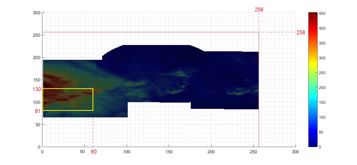
Figure 1: Two-dimensional image of precipitation data (data unit is mm) over a 512 km $\times$ 512 km region in the Brisbane area for two days (25th and 26th January 2013) and the selected area that specified by yellow rectangle.

Figure 2: Two-dimensional image of precipitation data for the selected area from Figure 1.

Let $X_{ij}$ be the value of precipitation on $ij$-th square with vertices in $(i,j),(i,j-1),(i-1,j),(i-1,j-1)$, where $i=1,\ldots,60$ and $j=1,\ldots,50$. Also let $X_{i.}=\sum_{k=1}^{50}X_{ik}$ denotes the accumulated precipitation on $i$-th vertical strip and $X_{.j}=\sum_{l=1}^{60}X_{lj}$ the accumulated precipitation on $j$-th horizontal strip, where $i=1,\ldots,60$ and $j=1,\ldots,50$. Table 1 and Table 2 show such amounts on successive vertical and horizontal strips respectively. By plotting accumulated precipitations in Figures 3 and 4, the corresponding scale intervals are detected by fitting some proper parabolas that their end points are shown with vertical red lines. These plots high-lights two characteristic features of DSI processes as the ratio of the length of successive scale intervals are nearly the same which is called scale parameter and having somehow similar dilation in successive scale intervals. In Figure 3 this method detects three successive scale intervals for the accumulated precipitation on vertical strips with end points $a_{1}=0$, $a_{2}=14$, $a_{3}=31$, $a_{4}=52$, and in Figure 4 it detects three successive scale intervals for the accumulated precipitation on horizontal strips with end points $b_{1}=0$, $b_{2}=10$, $b_{3}=23$, $b_{4}=40$. Following the estimation method for scale parameter in [27], we evaluate the corresponding time varying scale parameters by $\lambda_{1,n-1}=\frac{a_{n+1}-a_{n}}{a_{n}-a_{n-1}}$ and $\lambda_{2,n-1}=\frac{b_{n+1}-b_{n}}{b_{n}-b_{n-1}}$ for $n=2,3$. This leads to find $\Lambda_{1}:=(\lambda_{1,1},\lambda_{1,2})=(1.214,1.235)$ as the values of scale parameter for DSI process of accumulated precipitation on the vertical strips and $\Lambda_{2}:=(\lambda_{2,1},\lambda_{2,2})=(1.3,1.307)$ on the horizontal strips. So we estimate horizontal and vertical scale parameters as

$${\hat{\lambda}_{1}}=\frac{{\lambda}_{1,1}+{\lambda}_{1,2}}{2}=\frac{1.214+1.235}{2}=1.224,\>\>\>\>\>\>\>\>\>{\hat{\lambda}_{2}}=\frac{{\lambda}_{2,1}+{\lambda}_{2,2}}{2}=\frac{1.3+1.307}{2}=1.303.$$ (4.1)

				$X_{i.}$
11169	11448	11812	12174	12454	12620	12673	12673	12663	12636
12590	12545	12516	12499	12511	12567	12692	12855	13013	13201
13406	13561	13646	13694	13750	13802	13813	13754	13613	13460
13382	13409	13532	13696	13896	14138	14377	14560	14672	14730
14765	14788	14820	14876	14956	15051	15152	15235	15299	15365
15433	15496	15572	15687	15850	16044	16276	16536	16787	17009

Table 1: Sum of precipitation data on vertical strips as millimeters

				$X_{.j}$
10593	10964	11379	11862	12443	13051	13578	13927	14105	14187
14171	14131	14184	14395	14835	15431	16064	16638	17039	17179
17161	17257	17546	17927	18188	18246	18303	18371	18387	18451
18728	19068	19215	19214	19152	19194	19419	19634	19668	19491
19246	19017	18882	18772	18575	18340	18184	18045	17809	17553

Table 2: Sum of precipitation data on horizontal strips as millimeters

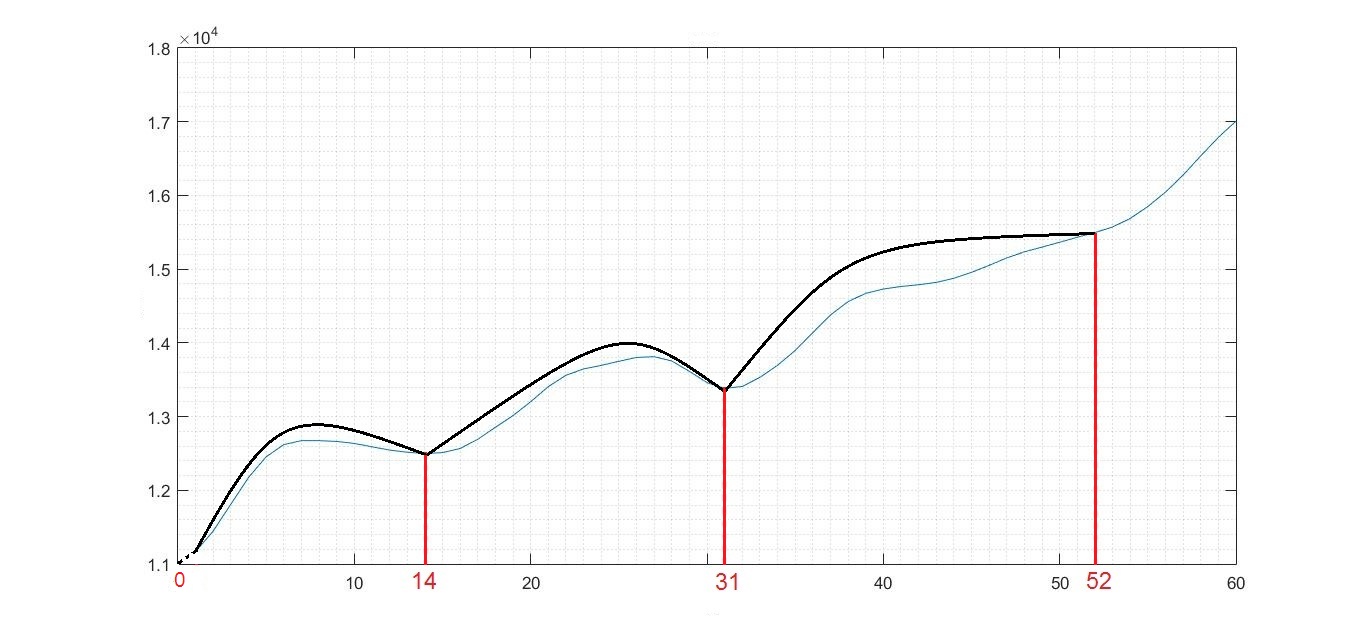
Figure 3: Fitted black curves for precipitation data on vertical strips and revealing the corresponding scale intervals by red lines.

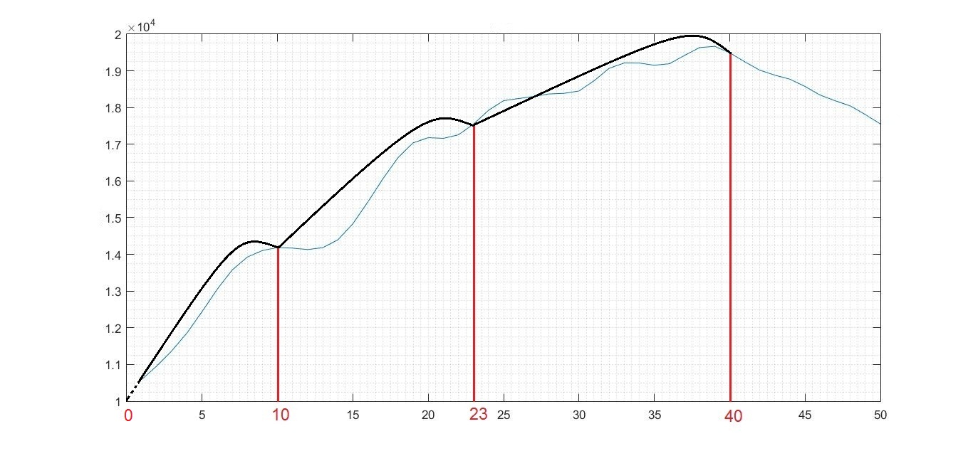
Figure 4: Fitted black curves for precipitation data on horizontal strips and revealing the corresponding scale intervals by red lines.

For each horizontal and vertical scale interval we consider two equal subintervals which are indicated with green dashed lines in Figures 5, 6. For the horizontal scale intervals, we partition each subinterval into seven equally length interval in Figure 5, where the accumulated precipitation on the corresponding successive vertical strips of the $m$-th subinterval of the $n$-th horizontal scale interval are denoted by $x_{(n,m)1},\ldots,x_{(n,m)7}$. So $x_{(n+1,m)k}\overset{\mathcal{L}}{=}\lambda_{1}^{\mathcal{H}_{(n,m)1}}x_{(n,m)k}$ where $\mathcal{H}_{(n,m)1}$ is corresponding Hurst parameter in between $n$-th and $(n+1)$-th horizontal scale intervals of sfBs (2.5) related to the $m$-th subintervals. Also each subinterval in vertical scale intervals is divided into five equally length interval in Figure 6, where the accumulated precipitation on the corresponding successive horizontal strips of the $m$-th subinterval of the $n$-th vertical scale interval are denoted by $y_{(n,m)1},\ldots,y_{(n,m)5}$. So $y_{(n+1,m)l}\overset{\mathcal{L}}{=}\lambda_{2}^{\mathcal{H}_{(n,m)2}}y_{(n,m)l}$ where $\mathcal{H}_{(n,m)2}$ is corresponding Hurst parameter in between $n$-th and $(n+1)$-th vertical scale intervals of sfBs (2.5) related to the $m$-th subintervals

4.2 Estimation of Hurst parameters

For the estimation of the Hurst parameters of fitted sfBs (2.5) to the precipitation area, using the notations described at the end of subsection 4.1, we have that

$$x_{(n+1,m)k}^{2}\overset{\mathcal{L}}{=}\lambda_{1}^{2\mathcal{H}_{(n,m)1}}x_{(n,m)k}^{2}$$

for $k=1,\ldots,7$ and

$$y_{(n+1,m)l}^{2}\overset{\mathcal{L}}{=}\lambda_{2}^{2\mathcal{H}_{(n,m)2}}y_{(n,m)l}^{2}$$

for $l=1,\ldots,5$. Now we propose to estimate $\lambda_{i}^{\mathcal{H}_{(n,m)i}}$ by the ratio of the corresponding quadratic means for $i=1,2$. Hence,

$$\hat{\mathcal{H}}_{(n,m)i}=\frac{\log(SS_{(n+1,m),i}/SS_{(n,m),i})}{2\log\lambda_{i,m}},$$

where

$$SS_{(n,m),1}=\frac{1}{7}\sum_{k=1}^{7}x^{2}_{(n,m)k},\>\>\>\>\>\>\>\>SS_{(n,m),2}=\frac{1}{5}\sum_{k=1}^{5}y^{2}_{(n,m)k}.$$ (4.2)

The values of $x_{(n,m)k}$ and $y_{(n,m)l}$ are presented in Tables 3 and 4 by $k$ orders.

n ​​​​​​	​​​ ​​​$x_{(n,1)k}$ ​​​​​​	​​​​​​$x_{(n,2)k}$
1 ​​​​​​	​​​​​​ 11169 - 11448 - 11812 - 12174 - 12454 - 12620 - 12673 ​​​​​​	​​​​​​ 12673 - 12663 - 12636 - 12590 - 12545 -12516 - 12499
2​​​ ​​​	​​​​​​15200 - 15310 - 15513 - 15754 - 16014 - 16319 - 16519 ​​​​​​	​​​​​​16601 - 16676 - 16753 - 16748 - 16617 -16406 - 16289
3​​​ ​​​	​​​​​​ 20175 - 20462 - 20965 - 21446 - 21896 - 22066 - 22159 ​​​​​​	​​​​​​22214 - 22354 - 22529 - 22770 - 22917 - 23082 - 23213

Table 3: precipitation values on partitions in subintervals along vertical strips.

n	$y_{(n,1)l}$	$y_{(n,2)l}$
1	10593 - 10964 - 11379 - 11862 - 12443	13051 - 13578 - 13927 - 14105 - 14187
2	18410 - 18402 - 18629 - 19361 - 20377	21342 - 22085 - 22326 - 22377 - 22723
3	30659 - 31024 - 31192 - 31309 - 31952	32592 - 32608 - 32761 - 33302 - 33259

Table 4: precipitation values on partitions in subintervals along horizontal strips.

The ratios of the mean squares and estimated Hurst values are shown in Tables 5 and 6.

n	$\frac{SS_{(n+1,1),1}}{SS_{(n,1),1}}$	$\hat{\mathcal{H}}_{(n,1)1}$	$\frac{SS_{(n+1,2),1}}{SS_{(n,2),1}}$	$\hat{\mathcal{H}}_{(n,2)1}$
1	1.718	1.40	1.736	1.42
2	1.819	1.42	1.878	1.49

Table 5: The ratios of squared of quadratic means and corresponding Hurst values along vertical strips.

n	$\frac{SS_{(n+1,1),2}}{SS_{(n,1),2}}$	$\hat{\mathcal{H}}_{(n,1)2}$	$\frac{SS_{(n+1,2),2}}{SS_{(n,2),2}}$	$\hat{\mathcal{H}}_{(n,2)2}$
1	2.76	1.93	2.60	1.81
2	2.69	1.85	2.20	1.47

Table 6: The ratios of squared of quadratic means and corresponding Hurst values along horizontal strips.

Hence,

Figure 5: Each horizontal scale interval is divided into two equally length subintervals by green dashed lines.

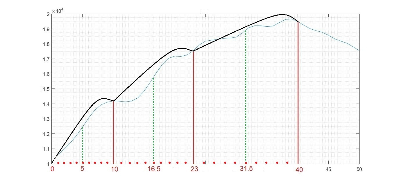
Figure 6: Each vertical scale interval is divided into two equally length subintervals by green dashed lines..

$$\hat{{\bf H}}_{1}:=(\hat{\mathcal{H}}_{(1,1)1},\hat{\mathcal{H}}_{(1,2)1},\hat{\mathcal{H}}_{(2,1)1},\hat{\mathcal{H}}_{(2,2)1})=(1.40,1.42,1.42,1.49)$$

and

$$\hat{{\bf H}}_{2}:=(\hat{\mathcal{H}}_{(1,1)2},\hat{\mathcal{H}}_{(1,2)2},\hat{\mathcal{H}}_{(2,1)2},\hat{\mathcal{H}}_{(2,2)2})=(1.93,1.81,1.85,1.47).$$

Denoting the Hurst parameter in between $n$-th and $(n+1)$-th horizontal scale intervals by $\hat{{{H}}}_{1,n}$ and for vertical scale intervals by $\hat{{{H}}}_{2,n}$, we have hat

$$\hat{{{H}}}_{1,1}=\frac{\hat{\mathcal{H}}_{(1,1)1}+\hat{\mathcal{H}}_{(1,2)1}}{2}=1.41,\>\>\>\>\>\>\hat{{{H}}}_{1,2}=\frac{\hat{\mathcal{H}}_{(2,1)1}+\hat{\mathcal{H}}_{(2,2)1}}{2}=1.46,$$

$$\hat{{{H}}}_{2,1}=\frac{\hat{\mathcal{H}}_{(1,1)2}+\hat{\mathcal{H}}_{(1,2)2}}{2}=1.87,\>\>\>\>\>\>\>\hat{{{H}}}_{2,2}=\frac{\hat{\mathcal{H}}_{(2,1)2}+\hat{\mathcal{H}}_{(2,2)2}}{2}=1.66.$$

So we estimate horizontal and vertical Hurst parameters of fitted sfBs (2.5) by

$$\small\hat{{{H}}}_{1}=\frac{\hat{{{H}}}_{1,1}+\hat{{{H}}}_{1,2}}{2}=\frac{1.41+1.46}{2}=1.435\>\>\>\>\>\>\>\hat{{{H}}}_{2}=\frac{\hat{{{H}}}_{2,1}+\hat{{{H}}}_{2,2}}{2}=\frac{1.87+1.66}{2}=1.765$$ (4.3)

Now we show the DSI behavior of the precipitation with respect to time in the selected whole area which is shown in Figure 2. For this, we consider the accumulated precipitation in this area for every 30 minutes on 25th and 26th January 2013 which are depicted in Table 7 by their orders of time.

2311	2568	2702	2802	2351	2248	2496	2552	2061	1780
1453	1823	2415	2596	2885	2947	2936	3113	2877	2974
3511	3954	2339	1525	1527	2071	2907	2545	1965	2310
3064	2455	1515	1516	1527	848	1837	2110	1064	975
1084	2163	4603	6409	6157	5246	4998	5610	3880	2292
4130	5911	8518	8876	9693	11377	10841	12442	14649	16939
15266	15964	15842	16711	17760	17274	15813	14470	13623	13521
14326	14867	16331	16070	15880	18072	21312	22709	24026	22112
21492	21567	16331	22416	23215	23309	21192	17992	17550	15295
13795	11567	9122	7488	6425	4745

Table 7: Values of the successive 30 minute precipitation data on the selected region in the Brisbane area for 25 and 26 January 2013 as millimeters.

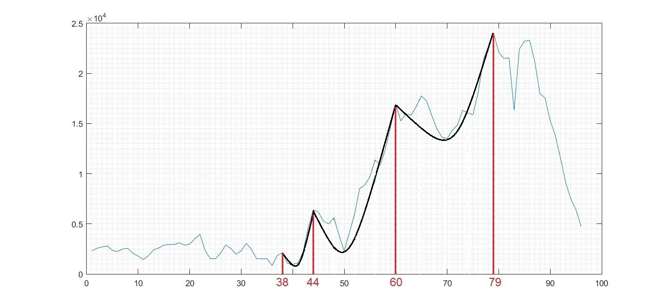
Figure 7: The fitted black curve shows the scale intervals of 30 minutes precipitation on 25th and 26th January 2013. Scale intervals are shown by red lines.

Figure 8: Each scale interval, for successive 30 minutes precipitation on 25-26 January 2013, is divided into two equally length subintervals by green dashed lines.

In Figure 7, precipitation per successive 30 minutes duration on the two days are plotted by blue. We fit some parabolas to the successive scale intervals in this figure and highlight the boundary of these scale intervals with red lines. So we have three scale intervals where the end points of these scale intervals are $c_{1}=38$, $c_{2}=44$, $c_{3}=60$, $c_{4}=79$. Thus, the scale parameter can be evaluated by $\lambda_{3,n-1}=\frac{c_{n+1}-c_{n}}{c_{n}-c_{n-1}}$ for $n=2,3$. So, we have $\Lambda_{3}:=(\lambda_{3,1},\lambda_{3,2})=(2.667,1.187)$. We divide each scale interval into two equal subintervals which are indicated with green dashed lines in Figure 8 and partition these subinterval with the equally spaced red points. Following the same method described at the beginning of the subsection 4.2, the Hurst parameters related to the $m$-th subintervals of the $n$-th and $(n+1)$-th scale intervals is estimated by

$${\mathcal{H}}_{(n,m)3}=\frac{\log(SS_{(n+1,m),3}/SS_{(n,m),3})}{2\log\lambda_{3,m}},$$

where $SS_{(n,m),3}=\frac{1}{3}\sum_{k=1}^{3}z^{2}_{(n,m)k}$, in which $z_{(n,m)1},z_{(n,m)2},z_{(n,m)3}$ are accumulated precipitation on successive partitions of $m$-th subinterval of the $n$-th scale interval (presented in Table 8), which their ratio and corresponding Hurst estimates are shown in Table 9.

n	$z_{(n,1)k}$	$z_{(n,2)k}$
1	1064  - 975  - 1084	2163  - 4603  - 6409
2	14702 - 11946 - 11577	23791  - 29619  - 39924
3	49746  - 54290  - 45448	46732  - 52502  - 71119

Table 8: precipitation values on partitions in subintervals.

n	$\frac{SS_{(n+1,1),3}}{SS_{(n,1),3}}$	$\hat{\mathcal{H}}_{(n,1)3}$	$\frac{SS_{(n+1,2),3}}{SS_{(n,2),3}}$	$\hat{\mathcal{H}}_{(n,2)3}$
1	151.28	2.56	45.37	1.94
2	15.19	7.93	3.29	3.48

Table 9: The ratios of squared of quadratic means and corresponding Hurst values.

Thus

$$\hat{{\bf H}}_{3}:=(\hat{\mathcal{H}}_{(1,1)3},\hat{\mathcal{H}}_{(1,2)3},\hat{\mathcal{H}}_{(2,1)3},\hat{\mathcal{H}}_{(2,2)3})=(2.56,1.94,7.93,3.48)$$

,

$$\hat{{H}}_{3,1}=\frac{\hat{\mathcal{H}}_{(1,1)3}+\hat{\mathcal{H}}_{(1,2)3}}{2}=2.25,\>\>\>\>\>\>\hat{{H}}_{3,2}=\frac{\hat{\mathcal{H}}_{(2,1)3}+\hat{\mathcal{H}}_{(2,2)3}}{2}=5.7\vspace{5mm}$$

and

$$\hat{{{H}}}_{3}=\frac{\hat{{{H}}}_{3,1}+\hat{{{H}}}_{3,2}}{2}=\frac{2.25+5.7}{2}=3.98.\vspace{5mm}$$

Simple fractional Brownian sheet : Parameter Estimation
Here we are to justify the structure of simple fractional Brownian sheet (sfBs), defined by (2.5), as a MSI field for the precipitation data of Figure 2. After detecting scale rectangles, the scale parameters $(\lambda_{1},\lambda_{2})$ are estimated by (4.1). By (4.3), we have that $\hat{{H}}_{1}=1.435$ and $\hat{{H}}_{2}=1.765$. As we have $m_{1}=14$ equally spaced samples in each horizontal scale intervals in Figure 5, and $m_{2}=10$ equally spaced samples in each vertical scale intervals in Figure 6. These samples provide some partitions for each interval. Let $x_{1(n,k)}$ be the sum of precipitation on the $k$-th vertical strips corresponding to the $k$-th partition of the $n$-th horizontal scale interval where $n=1,2,3$ and $k=1,\ldots,14$. Now we are to estimate the Hurst parameters of the two-dimensional fractional Brownian sheet $H^{\prime}_{1}$ and $H^{\prime}_{2}$ corresponding to sfBs (2.5). For this we consider quadratic variations of lengths two and one for horizontal scale intervals as

$$SS_{1(n,2)}=\frac{1}{[\frac{m_{1}}{2}]-1}\sum_{l=2}^{[\frac{m_{1}}{2}]}(x_{1(n,2l)}-x_{1(n,2l-2)})^{2},\>\>\>\>\>\>SS_{1(n,1)}=\frac{1}{[\frac{m_{1}}{2}]-1}\sum_{l=2}^{[\frac{m_{1}}{2}]}(x_{1(n,l)}-x_{1(n,l-1)})^{2}$$

and for vertical scale intervals as

$$SS_{2(n,2)}=\frac{1}{[\frac{m_{2}}{2}]-1}\sum_{l=2}^{[\frac{m_{2}}{2}]}(x_{2(n,2l)}-x_{2(n,2l-2)})^{2},\>\>\>\>\>\>SS_{2(n,1)}=\frac{1}{[\frac{m_{2}}{2}]-1}\sum_{l=2}^{[\frac{m_{2}}{2}]}(x_{2(n,l)}-x_{2(n,l-1)})^{2},$$

where $x_{2(n,k)}$ is the accumulated precipitation on the $k$-th horizontal strips corresponding to the $k$-th partition of the $n$-th vertical scale interval; $n=1,2,3$ and $k=1,\ldots,10$.
By component-wise self-similarity with Hurst $H_{i}^{{}^{\prime}}$ and component-wise stationary increment property of the samples inside each scale rectangle of sfBs; this is by the fact that when we consider accumulate precipitation on the strips and denote them by $x_{i(n,l)}$ they construct a simple fractional Brownian motion which inside each scale rectangles samples are just some multiple of a fractional Brownian motion and so have stationary increments, so we have that

$$(x_{i(n,2l)}-x_{i(n,2l-2)})\overset{\mathcal{L}}{=}2^{H_{i}^{{}^{\prime}}}(x_{i(n,l)}-x_{i(n,l-1)})$$ (4.4)

for $i=1,2$, and by MSI behavior of sfBs (2.5) we have that $x_{i(n,2l)}\overset{\mathcal{L}}{=}\lambda_{i}^{H_{i}}x_{i(n-1,2l)}$. So

$$SS_{i(1,2)}\overset{\mathcal{L}}{=}\frac{SS_{i(2,2)}}{{\lambda_{i}}^{2H_{i}}}\overset{\mathcal{L}}{=}\frac{SS_{i(3,2)}}{{\lambda_{i}}^{4H_{i}}},\;\;\;\;\;\;SS_{i(1,1)}\overset{\mathcal{L}}{=}\frac{SS_{i(2,1)}}{{\lambda_{i}}^{2H_{i}}}\overset{\mathcal{L}}{=}\frac{SS_{i(3,1)}}{{\lambda_{i}}^{4H_{i}}}$$

and by (4.4), $SS_{i(1,2)}\overset{\mathcal{L}}{=}2^{2H_{i}^{{}^{\prime}}}SS_{i(1,1)}$. Therefore by assuming

$$U_{i2}=SS_{i(1,2)}+\frac{SS_{i(2,2)}}{{\lambda_{i}}^{2H_{i}}}+\frac{SS_{i(3,2)}}{{\lambda_{i}}^{4H_{i}}},\>\>\>\>\>\>\>\>\>\>V_{i1}=SS_{i(1,1)}+\frac{SS_{i(2,1)}}{{\lambda_{i}}^{2H_{i}}}+\frac{SS_{i(3,1)}}{{\lambda_{i}}^{4H_{i}}},\>\>\>i=1,2,$$

we have that $U_{i2}\overset{\mathcal{L}}{=}2^{2H_{1i}^{{}^{\prime}}}V_{i1}$. Also we note that for $i=1,2$, $U_{i2}$ and $V_{i1}$ consist of $r_{i}([\frac{m_{i}}{2}]-1)$ increment samples where $r_{1}=r_{2}=3$ is the number of vertical or horizontal scale intervals and $m_{1}=14$ is the number of vertical strips in each horizontal scale interval and $m_{2}=10$ is the number of horizontal strips in each vertical scale interval. So by similar method to the theorem 1 of Rezakhah et al. [27] where used the result of Ayache et al [3] for fBm, we have the estimation of the Hurst parameters of sfBs as

$$\hat{H}_{1}^{{}^{\prime}}=\frac{\log(\frac{\hat{U}_{12}}{\hat{V}_{11}})}{2\log 2}=0.47,\>\>\>\>\>\>\>\>\>\>\>\>\hat{H}_{2}^{{}^{\prime}}=\frac{\log(\frac{\hat{U}_{22}}{\hat{V}_{21}})}{2\log 2}=0.91,$$

where

$$\hat{U}_{i2}=SS_{i(1,2)}+\frac{SS_{i(2,2)}}{{\lambda_{i}}^{2\hat{H}_{i}}}+\frac{SS_{i(3,2)}}{{\lambda_{i}}^{4\hat{H}_{i}}},\>\>\>\>\>\>\>\>\>\>\hat{V}_{i1}=SS_{i(1,1)}+\frac{SS_{i(2,1)}}{{\lambda_{i}}^{2\hat{H}_{i}}}+\frac{SS_{i(3,1)}}{{\lambda_{i}}^{4\hat{H}_{i}}}.$$

4.3 Prediction

For prediction we use component-wise (latitude and longitude) scale invariant property of sfBs model (2.5) assumed for the precipitation in Brisbane area of Australia on the specified duration of time (25 and 26 January 2013) depicted in Figure 2 to predict the values of precipitation on different region ($A_{ij}$) based on the values of the precipitation on the first region ($A_{11}$) in Figure 9. Here we study prediction of the precipitation in surface which are depicted in Figures 9 and 10. For this, first we denote the 9 scale rectangles as $A_{11},\ldots,A_{33}$ in Figure 9, which are in correspondence to the vertical and horizontal scale intervals presented in Figures 3 and 4. We partition each scale rectangle $A_{ij}$ into four sub-rectangles $A_{ij,k}$; $k=1,2,3,4$ in Figure 10 that are related to the sub-intervals in Figures 5 and 6. The scale sub-rectangles are shown in Figure 10 with black lines along vertical axis at points $d_{1}=0$, $d_{2}=7$, $d_{3}=14$, $d_{4}=22.5$, $d_{5}=31$, $d_{6}=41.5$, $d_{7}=52$ and along horizontal axis at points $e_{1}=0$, $e_{2}=5$, $e_{3}=10$, $e_{4}=16.5$, $e_{5}=23$, $e_{6}=31.5$, $e_{7}=40$. Let $(s_{1},t_{1}),(s_{2},t_{1}),(s_{1},t_{2})$ and $(s_{2},t_{2})$ denote the center points of the sub-rectangles $A_{11,1},A_{11,2},A_{11,3},A_{11,4}$. So for $i,j=1,2,3$ we denote the accumulated precipitation on sub-rectangles $A_{ij,1},A_{ij,2},A_{ij,3}$ and $A_{ij,4},$ which are recorded in Table 10, by $\,X(\lambda_{1}^{i-1}s_{1},\lambda_{2}^{j-1}t_{1}),\;X(\lambda_{1}^{i-1}s_{2},\lambda_{2}^{j-1}t_{1}),\;X(\lambda_{1}^{i-1}s_{1},\lambda_{2}^{j-1}t_{2})\;$ and $X(\lambda_{1}^{i-1}s_{2},\lambda_{2}^{j-1}t_{2}),$ related to their center points, respectively. Reffering to the Figure 10, we assume that the correlation of the accumulated precipitations on the corresponding sub-rectangles in the first and second vertical scale strips, say $(A_{1j,k},A_{2j,k})$, $\,j=1,2,3$ and $k=1,2,3,4$ to be the same. Also the correlation of the accumulated precipitations on corresponding sub-rectangles of the second and third vertical scale strips $(A_{2j,k},A_{3j,k})$ to be the same. Finally the accumulated precipitation on corresponding sub-rectangles of the first and third vertical scale strips $(A_{1j,k},A_{3j,k})$ have the same correlation. So using the notations of Remark 6 we estimate $R_{X_{1}^{*}}(2)$ by calculating the sample correlation of the accumulated precipitations on the pair of sub-rectangles $(A_{1j,k},A_{3j,k})$ as $0.9046$. The $R_{X^{*}_{1}}(1)$ can be estimated as the correlation of the accumulated precipitation on the pair of sub-rectangles $A_{1j,k},A_{2j,k}$ or on the pair of sub-rectangles $A_{2j,k},A_{3j,k}$ which are corresponding sub-rectangles in the first and second horizontal scale strips and in the second and third horizontal scale strips respectively and are evaluated as $-0.9573$ and $-0.9544$.

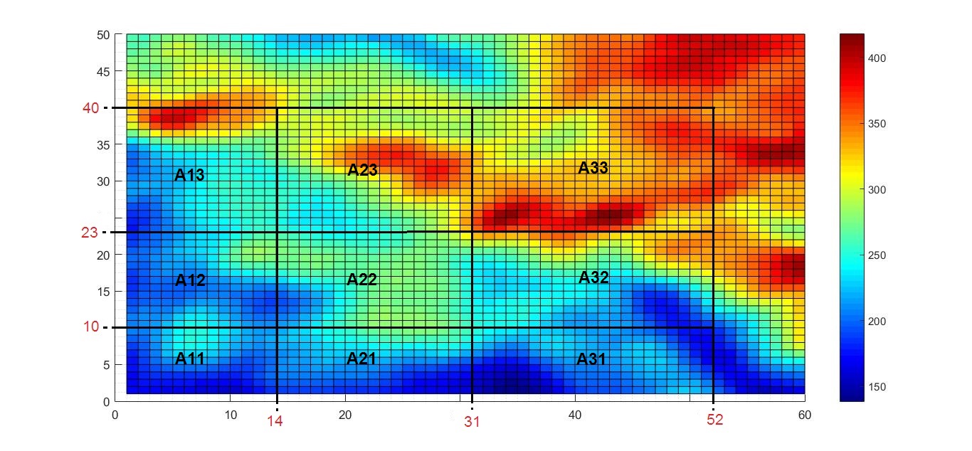
Figure 9: Nine rectangle areas, which are obtained by crossing lines along end points of scale intervals.

Figure 10: sub-rectangle areas, which are obtained by crossing lines along subinterval points of scale intervals.

sub-rectangular area	$A_{11,1}$	$A_{11,2}$	$A_{11,3}$	$A_{11,4}$	$A_{12,1}$	$A_{12,2}$	$A_{12,3}$	$A_{12,4}$	$A_{13,1}$
precipitation value	6451	6590	7816	7701	9314	9577	9572	11686	12983
sub-rectangular area	$A_{13,2}$	$A_{13,3}$	$A_{13,4}$	$A_{21,1}$	$A_{21,2}$	$A_{21,3}$	$A_{21,4}$	$A_{22,1}$	$A_{22,2}$
precipitation value	14915	18062	17882	8631	7761	10216	10733	13567	14716
sub-rectangular area	$A_{22,3}$	$A_{22,4}$	$A_{23,1}$	$A_{23,2}$	$A_{23,3}$	$A_{23,4}$	$A_{31,1}$	$A_{31,2}$	$A_{31,3}$
precipitation value	14370	15161	19372	23591	22272	22617	9300	10910	11715
sub-rectangular area	$A_{31,4}$	$A_{32,1}$	$A_{32,2}$	$A_{32,3}$	$A_{32,4}$	$A_{33,1}$	$A_{33,2}$	$A_{33,3}$	$A_{33,4}$
precipitation value	10428	16210	15111	20707	21592	31390	31123	27169	31183

Table 10: The accumulated precipitation value on the sub-rectangular regions.

Now following Remarks 5 and 6 we show that the precipitations has component-wise scale Markov property. Following notations of Remark 6, and the estimated values of $R_{X_{1}^{*}}(2)$ and $R_{X_{1}^{*}}(1)$ we estimate $\alpha_{Y_{1}}(2)$ as the partial auto-correlation function of $Y_{1}(\cdot)$ at lag 2 as $-0.1416$ and $-0.0707$ based on the two estimated values of $R_{X_{1}^{*}}(1)$ . As number of samples is 12 and both of these values are between $\pm 1.96/\sqrt{12}=\pm 0.5658$. Therefore, at level $\%95$ the first component scale Markov property for the precipitation is accepted. By the same method we evaluate the sample partial auto-correlation $\alpha_{Y_{2}}(2)$ of $Y_{2}$ at lag 2 is evaluated by estimating $R_{X_{2}^{*}}(2)$ and $R_{X_{2}^{*}}(1)$ which are estimated by using the accumulated precipitation on the pair of sub-rectangles $(A_{i1,k},A_{i3,k})$ and on pair of sub-rectangles $(A_{i1,k},A_{i2,k})$ or $(A_{i2,k},A_{i3,k})$ for $i=1,2,3$ and $k=1,2,3,4$ which cause the sample partial auto-correlation at lag 2, say $\alpha_{Y_{2}}(2)$, to be evaluated as $0.3242$ or $0.2624$ which both are between $\pm 1.96/\sqrt{12}=\pm 0.5658$. So at level $\%95$ it is accepted that $Y_{2}$ follows an AR(1) model. Thus by Remark 5 and Remark 6 of Section 3 the sfBs $X(t_{1},t_{2})$ of the accumulated precipitation on these sub-rectangles has component-wise scale Markov property. For the simplicity let $Y_{ij,k}$ denote the accumulated precipitation on sub-rectangle $A_{ij,k}$ for $i,j=1,2,3$ and $k=1,2,3,4$. So, the accumulated precipitation $Y_{ij,k}$ have component-wise Markov property in components $i$ and $j$ for fixed $k$. Also following MSI property, ${Y}_{ij,k}\overset{\mathcal{L}}{=}\lambda_{1}^{(i-1){H}_{1}}\lambda_{2}^{(j-1){H}_{2}}Y_{11,k}$ for $i,j=1,2,3$ and $k=1,2,3,4$ where $Y_{ij,k}$ as the accumulated precipitation on sub-rectangles $A_{ij,k}$ are shown in Figure 10 and their values are recorded in Table 10. Therefore under the assumption that the precipitation $Y_{11,k}$ is known, $Y_{ij,k}$ can be predicted using conditional expectation as

$$\hat{Y}_{ij,k|{11,k}}=\hat{E}[{Y}_{ij,k}|Y_{11,k}]=\hat{\lambda}_{1}^{(i-1){\hat{H}}_{1}}\hat{\lambda}_{2}^{(j-1){\hat{H}}_{2}}Y_{11,k}$$ (4.5)

for $i,j=1,2,3$ and $k=1,2,3,4$. Let $Y_{ij}=\sum_{i=k}^{4}Y_{ij,k}$ be the accumulated precipitation on the scale rectangular $A_{ij}$ for $i,j=1,2,3$ in Figure 9. So the prediction of $Y_{ij}$ provided the precipitation $Y_{11,k};k=1,2,3,4$ is known can be evaluated as $\sum_{k=1}^{4}\hat{Y}_{ij,k|{11,k}}$ (Table 11). The real precipitation on $A_{ij}$ ($Y_{ij}$) and corresponding predicted value are plotted in Figure 11.

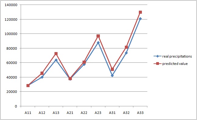
Figure 11: The accumulated precipitation value and corresponding predicted value on rectangular regions.

rectangular area ​​​​	$A_{11}$	$A_{12}$	$A_{13}$	$A_{21}$	$A_{22}$	$A_{23}$	$A_{31}$	$A_{32}$	$A_{33}$
precipitation values ​​​​	28558	40149	63842	37341	57814	87852	42353	73620	120865
predicted values	28558	45562	72691	38168	60894	97151	51011	81384	129842

Table 11: The accumulated precipitation value and corresponding predicted value on rectangular regions.

The mean absolute percentage error (MAPE) is a famous measure for the prediction accuracy, [9, 17, 24], is defined by

$$\gamma=\frac{1}{n}\sum_{i=1}^{n}|\frac{r_{i}-\hat{r}_{i}}{r_{i}}|\times 100,$$

where $r_{i}$ and $\hat{r}_{i}$ are respectively real value and predicted value for $i$-th data point and $n$ is the number of data points. According to interpretation of MAPE values by Lewis[19], for highly accurate forecasting $\gamma\leq 10$, good forecasting $10<\gamma\leq 20$, reasonable forecasting $20<\gamma\leq 50$ and for inaccurate forecasting $\gamma>50$, see Moreno et al. [24].
So we consider MAPE as an accuracy index for the predicted values on eight rectangular areas in Figure 9. The MAPE value for these data is evaluated as

$$\gamma^{*}=\frac{1}{8}\sum_{k=1}^{3}\sum_{l=1}^{3}|\frac{{Y}_{kl}-\hat{Y}_{kl}}{Y_{kl}}|\times 100,$$ (4.6)

where $\hat{Y}_{11}$ is equal to $Y_{11}$ and is ignored in calculations, because the rectangular region $A11$ is the initial region. Table 12 shows the absolute values in (4.6).

rectangular area	$A_{11}$	$A_{12}$	$A_{13}$	$A_{21}$	$A_{22}$	$A_{23}$	$A_{31}$	$A_{32}$	$A_{33}$
absolute value	0	0.135	0.139	0.022	0.053	0.106	0.204	0.105	0.074

Table 12: Absolute of difference between the actual precipitation values and the corresponding predicted values are divided by the actual precipitation values.

These values are absolute of difference between the actual accumulated precipitation values on nine rectangular regions and the corresponding predicted values divided by the actual accumulated precipitation values. The MAPE value is obtained as $\gamma^{*}=10.5$.
Hence, by Lewis’s classification for MAPE values, this is a verified certificate for the accuracy of our prediction method of precipitation values.

One could follow the method of this section to predict the precipitation in time while we have the same circumstances (as the DSI behavior always valid for restricted duration) by having the precipitation in some scale interval of time. Prediction can be followed in surface and time simultaneously by applying these predictions successively.

5 Discussion $\&$ Conclusions

In this paper, we have introduced multi-scale invariant (MSI) fields which have component-wise discrete scale invariant property. It is shown that the covariance function of the MSI field with Markov property (MMSI) is characterized by the covariance functions and variances of samples on the first scale rectangle. A two-dimensional simple fractional Brownian sheet (sfBs) as an example of MSI field is demonstrated and applied to a set of real data, say precipitation in Brisbane area of Australia and considered prediction that its high accuracy is shown by using MAPE method.
Regarding Markov property of MSI field, even though assuming Markov property for the precipitation on different parts of some area is not so realistic but this can be a property in some other MSI fields. Results of section 3 enables one to evaluate the covariance structure between samples of any two scale rectangles of Markov MSI field (3.4) by using the covariance structure and variance functions of samples inside first scale interval.

Acknowledgment
We would like to express our sincere thanks to the two anonymous reviewers that their valuable comments helped us to improve the quality of this manuscript. The authors would like to express their thanks to Professor Alan Seed from Australian Bureau of Meteorology for providing the data used in this paper.

References

- [1] N. M. Aarato. Mean Estimation of Brownian Sheet. Computers Math. Applic. 33(8), 13-25, 1997.
- [2] K. O. Aiyesimoju and A. O. Busari. A multi-period Markov model for monthly rainfall in Lagos, Nigeria. Journal of Science and Technology. 35 (3), 25-33, 2015.
- [3] A. Ayache, P. Bertrand, and J. Levy Vehel. A Central limit theorem for the generalized quadratic variation of the step fractional Brownian motion. Statistical Inference for Stochastic Processes 10 (1), 1-27, 2007.
- [4] G. Balasis, I. A. Daglis, A. Anastasiadis and K. Eftaxias, Detection of dynamical complexity changes in Dst time series using entropy concepts and rescaled range analysis, in The Dynamic Magnetosphere, IAGA Special Sopron Book Series, Vol. 3 , Springer 2011, pp. 211-220.
- [5] G. Balasis, I. A. Daglis, C. Papadimitriou, M. Kalimeri, A. Anastasiadis and K. Eftaxias, Investigating dynamical complexity in the magnestosphere using various entropy measures, J. Geophys. Res. 114 (2009) A00D06.
- [6] G. Balasis, C. Papadimitriou, I. A. Daglis, A. Anastasiadis, L. Athanasopoulou and K. Eftaxias, Signatures of discrete scale invariance in Dst time series, Geophys. Res. Lett. 38, L13103/1-6, doi: 10.1029/2011GL048019 , 2011
- [7] M. Bartolozzi, S. Drozdz, D. B. Leieber, J. Speth and A. W. Thomas, Self-similar log-periodic structures in Western stock markets from 2000, Int. J. Mod. Phys. C. 16(9), 1347–1361, 2005.
- [8] P. Borgnat, P. Flandrin and P.O. Amblard. Stochastic discrete scale invariance. IEEE Signal Processing Letters. 9(6), 181-184, 2002.
- [9] B. L. Bowerman, R. T. O’Connell, A. B. Koehler. Forecasting, time series and regression: An applied approach. Thomson Brooks/Cole, Belmont, CA, 2004.
- [10] P. A. Brockwell, R. A. Davis. Time series: Theory and methods. Second ed, Springer, NY, 2006.
- [11] A. Cancelliere and J. D. Sallas. Drought length properties of periodic-stochastic hydrologic data. Water resources research. 40, w02503, 2004.
- [12] C. Chatfield and H. Xing. The analysis of time Series analysis. Seventh ed, Chapman Hall, FL, 2019.
- [13] Commonwealth of Australia, Bureau of Meteorology (ABN 92 637 533 532), http://www.bom.gov.au/other/copyright.shtml.
- [14] M. Fuentes. Testing for separability of spatial- temporal covariance functions. Journal of Statistical Planning and inference. 136, 447-466, 2006.
- [15] M.G. Genton, O. Perrin and M.S. Taqqu. Self-Similarity and Lamperti transformation for random fields. Stochastic Models. 23, 397-411, 2007.
- [16] M.G. Genton. Separable approximations of space-time covariance matrices. Environmetrics. 18, 681-695, 2007.
- [17] J.E. Hanke, A.G. Reitsch. Business forecasting (5th ed.), Prentice-Hall, Englewood Cliffs, NJ, 1995.
- [18] H. Hurd, G. Kallianpur and J. Farshidi. Correlation and spectral theory for periodically correlated random fields indexed on . Journal of Multivariate Analysis. 90, 359-383, 2004.
- [19] C.D. Lewis. Industrial and business forecasting methods. London: Butterworths, 1982.
- [20] V. Makogin, Y. Mishura. Example of a Gaussian self-similar field with stationary rectangular increments that is not a fractional Brownian sheet. Stochastic Analysis and Applications. 33(3), 413-428, 2015.
- [21] N. Modarresi and S. Rezakhah. Spectral analysis of multi-dimensional self-similar Markov processes. J. Phys. A, Math. Theor. 43(12), 125004 , 14 pp, 2010.
- [22] N. Modarresi and S. Rezakhah. A new structure for analyzing discrete scale invariant processes: covariance and spectra. J. Stat. Phys. 153, 162-176, 2013.
- [23] N. Modarresi and S. Rezakhah. Characterization of discrete scale invariant Markov sequences. Communications in Statistics: Theory and Methods. 45(18), 5263 -5278, 2016.
- [24] J.J.M. Moreno, A.P. Pole, A.S. Abad, B.C. Blasco. Using the R-MAPE index as a resistant measure of forecast accuracy. Psicothema. 25(4), 500-506, 2013.
- [25] C.J. Nuzman and H.V. Poor. Linear estimation of self-similar processes via Lamperti transformation. Journal of Applied Probability. 37(2), 2000.
- [26] T.O. Olatayo and A.I. Taiwo. Statistical modelling and prediction of rainfall time series data. Global Journal of Comuter Science and Technology (G). 14(1), 1-10, 2014.
- [27] S. Rezakhah, A. Philippe and N. Modarresi. Innovative methods for modeling of scale invariant processes. Communications in Statistics-Theory and Methods. 47(13), 3178-3191, 2017.
- [28] S. Rezakhah and Y. Maleki. Discretization of continuous time discrete scale invariant processes: estimation and spectra. J. Stat. Phys. 164, 438-448, 2016.
- [29] A. Rosenfeld and A.C. Kak. Digital Picture Processing. Second ed, Vol. 1, Academic Press, New York, 1982.
- [30] Y.A. Rozanov. Stationary Random Processes. Holden Day, San Francisco, 1967.
- [31] G. Samorodnitsky and M.S. Taqqu. Stable Non-Gaussian Random Processes: Stochastic Models with Infinite Variance, Stochastic Modeling. Chapman and Hall, New York, 1994.
- [32] G. Tian and Y. C. Tian. Markov modelling of the IEEE 802.11 DCF for real-time applications with periodic traffic. IEEE 12th International Conference on High Performance Computing and Communications (HPCC), Melbourne . VIC, 6(3), 419-426, 2010.
- [33] G.A. Tularam and M. Ilahee. Time series analysis of rainfall and temperature interactions in coastal catchments. Journal of Mathematics and Statistics. 6(3), 372-380, 2010.
- [34] W. Wang. Almost-sure path properties of fractional Brownian sheet, Annales de l’Institut Henri Poincare (B) Probability and Statistics, 43(5): 619-631, 2007.
- [35] D. Wu and Y. Xiao. Geometric properties of fractional Brownian sheets. J. Fourier Anal. Appl. 13(1), 1-37, 2007.