Construction of Kuranishi structures on the moduli spaces of pseudo holomorphic disks: I

Abstract.

This is the first of two articles in which we provide detailed and self-contained account of the construction of a system of Kuranishi structures on the moduli spaces of pseudo holomorphic disks, using the exponential decay estimate given in [FOOO7]. This article completes the construction of a Kuranishi structure of a single moduli space. This article is an improved version of [FOOO4, Part 4] and its mathematical content is taken from our earlier writing [FOn, FOOO2, FOOO4, FOOO7].

Oct. 03st, 2017

1. Statement of the results

This is the first of two articles which provide detail of the construction of a system of Kuranishi structures on the moduli spaces of pseudo holomorphic disks.

The construction of Kuranishi structure on the moduli spaces of pseudo holomorphic curves is a part of the virtual fundamental chain/cycle technique which was discovered in the year 1996 ([FOn, LiTi, LiuTi, Ru, Sie]). The case of pseudo holomorphic disks was established and used in [FOOO1, FOOO2].

Let $(X,\omega)$ be a symplectic manifold that is tame at infinity and $L$ a compact Lagrangian submanifold without boundary. Take an almost complex structure $J$ on $X$ which is tamed by $\omega$ and let $\beta\in H_{2}(X,L;{\mathbb{Z}})$.

We denote by $\mathcal{M}_{k+1,\ell}(X,L,J;\beta)$ the compactified moduli space of stable maps with boundary condition given by $L$ and of homology class $\beta$, from marked disks with $k+1$ boundary and $\ell$ interior marked points. We require that the enumeration of the boundary marked points respects the cyclic order of the boundary. (See Definition 1.2 for the detail of this definition.) We can define a topology on $\mathcal{M}_{k+1,\ell}(X,L,J;\beta)$ which is Hausdorff and compact. (See [FOn, Definition 10.3], [FOOO2, Definition 7.1.42], and Definition 4.12.) The main result we prove in this article is as follows.

Theorem 1.1.

$\mathcal{M}_{k+1,\ell}(X,L,J;\beta)$ carries a Kuranishi structure with corners.

See Section 6 for the definition of Kuranishi structure.

This article is not an original research paper but is a revised version of [FOOO4, Part 4]. Most of the material of this article is taken from our previous writing such as [FOn, FOOO2, FOOO4, FOOO5, FOOO6, FOOO7, FOOO3, Fu1]. The novel points of this article are on its presentation and simplifications of the proofs especially in the following two points.

Firstly we clarify a sufficient condition of the way to take a family of ‘obstruction spaces’ so that it produces Kuranishi structure. In other word, we define the notion of obstruction bundle data (Definition 5.1) and show that we can associate a Kuranishi structure to given obstruction bundle data in a canonical way (Theorem 7.1). We also prove the existence of such obstruction bundle data (Theorem 11.1).

Secondly we use an ‘ambient set’ to simplify the construction of coordinate change and the proof of its compatibility. (See Remark 7.9 (2).)

This article studies a single moduli space and constructs its Kuranishi structure. We provide the detail of the proof using the exponential decay estimate in [FOOO7].

In the second of this series of articles, we will provide detail of the construction of a system of Kuranishi structures of the moduli spaces of holomorphic disks so that they are compatible. More precisely we will construct a tree like K-system as defined in [FOOO6, Definition 21.9].

We conclude the introduction by reviewing the definition of the moduli space $\mathcal{M}_{k+1,\ell}(X,L,J;\beta)$.

Definition 1.2.

Let $k,\ell\in{\mathbb{Z}}_{\geq 0}$. We denote by $\mathcal{M}_{k+1,\ell}(X,L,J;\beta)$ the set of all $\sim$ equivalence classes of $((\Sigma,\vec{z},\vec{\mathfrak{z}}),u)$ with the following properties.

1. $\Sigma$ is a genus $0$ bordered curve with one boundary component which has only (boundary or interior) nodal singularities.

2. $\vec{z}=(z_{0},z_{1},\dots,z_{k})$ is a $(k+1)$-tuple of boundary marked points. We assume that they are distinct and are not nodal points. Moreover we assume that the enumeration respects the counter clockwise cyclic ordering of the boundary.

3. $\vec{\mathfrak{z}}=({\mathfrak{z}}_{1},\dots,{\mathfrak{z}}_{\ell})$ is an $\ell$-tuple of interior marked points. We assume that they are distinct and are not nodal.

4. $u:(\Sigma,\partial\Sigma)\to(X,L)$ is a continuous map which is pseudo holomorphic on each irreducible component. The homology class $u_{*}([\Sigma,\partial\Sigma])$ is $\beta$.

5. $((\Sigma,\vec{z},\vec{\mathfrak{z}}),u)$ is stable in the sense of Definition 1.3 below.

We define an equivalence relation $\sim$ in Definition 1.3 below.

Definition 1.3.

Suppose $((\Sigma,\vec{z},\vec{\mathfrak{z}}),u)$ and $((\Sigma^{\prime},\vec{z}^{\,\prime},\vec{\mathfrak{z}}^{\,\prime}),u^{\prime})$ satisfy Definition 1.2 (1)(2)(3)(4). We call a homeomorphism $v:\Sigma\to\Sigma^{\prime}$ an extended isomorphism if the following holds.

1. $v$ is biholomorphic on each irreducible component.

2. $u^{\prime}\circ v=u$.

3. $v(z_{j})=z^{\prime}_{j}$ and there exists a permutation $\sigma:\{1,\dots,\ell\}\to\{1,\dots,\ell\}$ such that $(v({\mathfrak{z}}_{1}),\dots,v({\mathfrak{z}}_{\ell}))$ coincides with $({\mathfrak{z}}_{\sigma(1)},\dots,{\mathfrak{z}}_{\sigma(\ell)})$.

We call $v$ an isomorphism if $\sigma={\rm id}$ in addition and $((\Sigma,\vec{z},\vec{\mathfrak{z}}),u)\sim((\Sigma^{\prime},\vec{z}^{\,\prime},\vec{\mathfrak{z}}^{\,\prime}),u^{\prime})$ if there exists an isomorphism between them.

The group ${\rm Aut}^{+}((\Sigma,\vec{z}),\vec{\mathfrak{z}}),u)$ of extended automorphisms (resp. ${\rm Aut}((\Sigma,\vec{z},\vec{\mathfrak{z}}),u)$ of automorphisms) consists of extended isomorphisms (resp. isomorphisms) from $((\Sigma,\vec{z}),\vec{\mathfrak{z}}),u)$ to itself.

The object $((\Sigma,\vec{z},\vec{\mathfrak{z}}),u)$ is said to be stable if ${\rm Aut}^{+}((\Sigma,\vec{z},\vec{\mathfrak{z}}),u)$ is a finite group.

The whole construction of this article is invariant under the group of extended automorphisms. Therefore the Kuranishi structure in Theorem 1.1 is invariant under the permutation of the interior marked points.

2. Universal family of marked disks and spheres

In this section we review well-known facts about the moduli spaces of marked spheres and disks. See [DM, ACG, Ke] for the detail of the sphere case and [FOOO2, Subsection 7.1.5] for the detail of the disk case.

Proposition 2.1.

Let $\ell\geq 3$. There exist complex manifolds $\mathcal{M}^{\rm s,reg}_{\ell}$, $\mathcal{C}^{\rm s,reg}_{\ell}$ and holomorphic maps

$$\pi:\mathcal{C}^{\rm s,reg}_{\ell}\to\mathcal{M}^{\rm s,reg}_{\ell},\qquad\mathfrak{s}_{i}:\mathcal{M}^{\rm s,reg}_{\ell}\to\mathcal{C}^{\rm s,reg}_{\ell}$$

$i=1,\dots,\ell$, with the following properties.

1. $\pi$ is a proper submersion and its fiber $\pi^{-1}({\bf p})$ is biholomorphic to Riemann sphere $S^{2}$.

2. $\pi\circ\mathfrak{s}_{i}$ is the identity.

3. $\mathfrak{s}_{i}({\bf p})\neq\mathfrak{s}_{j}({\bf p})$ for $i\neq j$.

4. Let ${\mathfrak{z}}_{1},\dots,{\mathfrak{z}}_{\ell}\in S^{2}$ be mutually distinct points. Then there exists uniquely a point ${\bf p}\in\mathcal{M}^{\rm s,reg}_{\ell}$ and a biholomorphic map $S^{2}\to\pi^{-1}({\bf p})$ which sends ${\mathfrak{z}}_{i}$ to $\mathfrak{s}_{i}({\bf p})$.

5. There exist holomorphic actions of symmetric group ${\rm Perm}(\ell)$ of order $\ell!$ on $\mathcal{M}^{\rm s,reg}_{\ell}$, $\mathcal{C}^{\rm s,reg}_{\ell}$, which commute with $\pi$ and

   $$\mathfrak{s}_{\sigma(i)}(\sigma({\bf p}))=\sigma(\mathfrak{s}_{i}({\bf p})).$$

6. There exist anti-holomorphic involutions $\tau$ on $\mathcal{M}^{\rm s,reg}_{\ell}$, $\mathcal{C}^{\rm s,reg}_{\ell}$ such that $\pi$ and $\mathfrak{s}_{i}$ commute with $\tau$. The involution $\tau$ commutes with the action of ${\rm Perm}(\ell)$.

This is well-known and is easy to show.

We can compactify the universal family given in Proposition 2.1 as follows.

Theorem 2.2.

There exist compact complex manifolds $\mathcal{M}^{\rm s}_{\ell}$, $\mathcal{C}^{\rm s}_{\ell}$ containing $\mathcal{M}^{\rm s,reg}_{\ell}$, $\mathcal{C}^{\rm s,reg}_{\ell}$ as dense subspaces, respectively. The maps $\pi$ and $\mathfrak{s}_{i}$ extend to

$$\pi:\mathcal{C}^{\rm s}_{\ell}\to\mathcal{M}^{\rm s}_{\ell},\qquad\mathfrak{s}_{i}:\mathcal{M}^{\rm s}_{\ell}\to\mathcal{C}^{\rm s}_{\ell}$$

and the following holds.

1. $\pi$ is proper and holomorphic. For each point $x\in\mathcal{C}^{\rm s}_{\ell}$ at which $\pi$ is not a submersion, we may choose local coordinates so that $\pi$ is given locally by $(u_{1},\dots,u_{m},w_{1},w_{2})\to(u_{1},\dots,u_{m},w_{1}w_{2})$ where $m=\dim_{{\mathbb{C}}}\mathcal{M}^{\rm s}_{\ell}=\ell-3$.

2. $\pi\circ\mathfrak{s}_{i}$ is the identity. $\pi$ is a submersion on the image of $\mathfrak{s}_{i}$.

3. There exist holomorphic actions of symmetric group ${\rm Perm}(\ell)$ of order $\ell!$ on $\mathcal{M}^{\rm s}_{\ell}$, $\mathcal{C}^{\rm s}_{\ell}$, which commute with $\pi$ and

   $$\mathfrak{s}_{\sigma(i)}(\sigma({\bf p}))=\sigma(\mathfrak{s}_{i}({\bf p})).$$

4. There exist anti-holomorphic involutions $\tau$ on $\mathcal{M}^{\rm s}_{\ell}$, $\mathcal{C}^{\rm s}_{\ell}$ such that $\pi$ and $\mathfrak{s}_{i}$ commute with $\tau$. $\tau$ also commutes with the action of ${\rm Perm}(\ell)$.

This is a special case of the marked version of Deligne-Mumford’s compactification of the moduli space of stable curves ([DM]). We can make a similar statement as Proposition 2.1 (4), where we replace $(S^{2},(\mathfrak{z}_{1},\dots,\mathfrak{z}_{\ell}))$ by a stable marked curve $(\Sigma,\vec{\mathfrak{z}})$ of genus $0$ with $\ell$ marked points.

We next define the moduli space of marked disks. Let $k,\ell\in{\mathbb{Z}}_{\geq 0}$. We define

$$\rho_{0}:\{0,1,\dots,k+2\ell\}\to\{0,1,\dots,k+2\ell\}$$

as follows:

$$\rho_{0}(i)=i, \text{$i=0,\dots,k$},$$

$$\rho_{0}(k+2j-1)=k+2j, \text{$j=1,\dots,\ell$},$$

$$\rho_{0}(k+2j)=k+2j-1, \text{$j=1,\dots,\ell$}.$$

$\rho_{0}$ defines a holomorphic involution on ${\mathcal{M}}^{\rm s}_{k+2\ell+1}$. We compose it with $\tau$ and obtain an anti-holomorphic involution on ${\mathcal{M}}^{\rm s}_{k+2\ell+1}$, which we denote by $\tilde{\tau}$. We denote an element ${\bf p}\in{\mathcal{M}}^{\rm s}_{k+2\ell+1}$ by $(\pi^{-1}({\bf p}),\vec{\mathfrak{z}},\vec{\mathfrak{z}}^{\,+}({\bf p}),\vec{\mathfrak{z}}^{\,-}({\bf p}))$. Here

$$\vec{\mathfrak{z}}({\bf p}) =(\mathfrak{s}_{0}({\bf p}),\dots,\mathfrak{s}_{k}({\bf p})),$$

$$\vec{\mathfrak{z}}^{\,+}({\bf p}) =(\mathfrak{s}_{k+1}({\bf p}),\dots,\mathfrak{s}_{k+2j-1}({\bf p}),\dots,\mathfrak{s}_{k+2\ell-1}({\bf p}))$$

$$\vec{\mathfrak{z}}^{\,-}({\bf p}) =(\mathfrak{s}_{k+2}({\bf p}),\dots,\mathfrak{s}_{k+2j}({\bf p}),\dots,\mathfrak{s}_{k+2\ell}({\bf p}))$$

(Here we enumerate $\mathfrak{s}_{i}:{\mathcal{M}}^{\rm s}_{k+2\ell+1}\to{\mathcal{C}}^{\rm s}_{k+2\ell+1}$ by $i=0,\dots,k+2\ell$ in place of $i=1,\dots,k+2\ell+1$.)

We lift $\tilde{\tau}$ to ${\mathcal{C}}^{\rm s}_{k+2\ell+1}$ as follows. Note ${\mathcal{C}}^{\rm s}_{k+2\ell+1}$ is identified with ${\mathcal{M}}^{\rm s}_{k+2\ell+2}$, where the projection ${\mathcal{C}}^{\rm s}_{k+2\ell+1}\to{\mathcal{M}}^{\rm s}_{k+2\ell+1}$ is identified with the map ${\mathcal{M}}^{\rm s}_{k+2\ell+2}\to{\mathcal{M}}^{\rm s}_{k+2\ell+1}$ which forgets the last marked point. We extend $\rho_{0}$ to $\rho_{1}:\{0,1,\dots,k+2\ell+1\}\to\{0,1,\dots,k+2\ell+1\}$ by $\rho_{1}(k+2\ell+1)=k+2\ell+1$. The composition of $\tau:{\mathcal{M}}^{\rm s}_{k+2\ell+2}\to{\mathcal{M}}^{\rm s}_{k+2\ell+2}$ and $\rho_{1}$ is an anti-holomorphic involution $\tilde{\tau}$ on ${\mathcal{C}}^{\rm s}_{k+2\ell+1}$ which is a lift of the involution $\tilde{\tau}$ on ${\mathcal{M}}^{\rm s}_{k+2\ell+1}$

Suppose $\tilde{\tau}{\bf p}={\bf p}$, ${\bf p}\in{\mathcal{M}}^{\rm s,\rm{reg}}_{k+2\ell+1}$. Put $S^{2}_{\bf p}=\pi^{-1}({\bf p})$. The restriction of $\tilde{\tau}$, still denoted by $\tilde{\tau}$, becomes an anti-holomorphic involution $\tilde{\tau}$ on $S^{2}_{\bf p}$.

Note $\tilde{\tau}({\mathfrak{z}}_{0})={\mathfrak{z}}_{0}$ by definition. Therefore the fixed point set of the anti-holomorphic involution $\tilde{\tau}:S^{2}_{\bf p}\to S^{2}_{\bf p}$ is nonempty. We put $C_{\bf p}=\{z\in S^{2}_{\bf p}\mid\tilde{\tau}({\bf p})={\bf p}\}$. Using the fact $C_{\bf p}$ is nonempty we can show that $C_{\bf p}$ is a circle.

Definition 2.3.

We denote by ${\mathcal{M}}^{\rm d,reg}_{k+1,\ell}$ the set of all ${\bf p}\in{\mathcal{M}}^{\rm s,reg}_{k+2\ell+1}$ with the following properties.

1. $\tilde{\tau}{\bf p}={\bf p}$.

2. Let $C_{\bf p}$ be as above. We can decompose $S^{2}\setminus C_{\bf p}={\rm Int}D_{+}\cup{\rm Int}D_{-}$, where $D_{\pm}={\rm Int}D_{\pm}\cup C_{\bf x}$ are disks.

3. We require that elements of $\vec{\mathfrak{z}}^{+}$ are all in ${\rm Int}D_{+}$. (It implies that elements of $\vec{\mathfrak{z}}^{-}$ are all in ${\rm Int}D_{-}$.)

4. We orient $C_{\bf p}$ by using the (complex) orientation of ${\rm Int}D_{+}$. Note ${\mathfrak{z}}_{0},\dots,{\mathfrak{z}}_{k}\in C_{\bf p}$. We require the enumeration ${\mathfrak{z}}_{0},\dots,{\mathfrak{z}}_{k}$ respects the orientation of $C_{\bf p}$.

We denote by ${\mathcal{M}}^{\rm d}_{k+1,\ell}$ the closure of ${\mathcal{M}}^{\rm d,reg}_{k+1,\ell}$ in ${\mathcal{M}}^{\rm s}_{k+1+2\ell}$.

We remark that by definition ${\mathcal{M}}^{\rm d,reg}_{k+1,\ell}$ is a connected component of the fixed point set of the $\tilde{\tau}$ action of ${\mathcal{M}}^{\rm s,reg}_{k+2\ell+1}$. We also remark that ${\mathcal{M}}^{\rm d,reg}_{k+1,\ell}$ is identified with the set of isomorphism classes of $(D^{2},\vec{z},\vec{\mathfrak{z}})$ where:

1. $\vec{z}=(z_{0},\dots,z_{k+1})$, $z_{j}\in\partial D^{2}$ are mutually distinct and the enumeration respects the orientation.

2. $\vec{\mathfrak{z}}=({\mathfrak{z}}_{1},\dots,{\mathfrak{z}}_{\ell})$, ${\mathfrak{z}}_{i}\in{\rm Int}D^{2}$ are mutually distinct.

We say $(D^{2},\vec{z},\vec{\mathfrak{z}})$ is isomorphic to $(D^{2},\vec{z}^{\,\prime},\vec{\mathfrak{z}}^{\,\prime})$ if there exists a biholomorphic map $v:D^{2}\to D^{2}$ such that $v(z_{i})=z^{\prime}_{i}$ and $v({\mathfrak{z}}_{i})={\mathfrak{z}}^{\prime}_{i}$.

We can use this remark to show the identification:

$${\mathcal{M}}^{\rm d}_{k+1,\ell}\cong\mathcal{M}_{k+1,\ell}({\rm pt},{\rm pt},J;0).$$

Here the right hand side is the case of the moduli space $\mathcal{M}_{k+1,\ell}(X,L,J;\beta)$ when $X$ is a point. ($L$ then is necessarily a point and the homology class $\beta$ is $0$.) Therefore an element of ${\mathcal{M}}^{\rm d}_{k+1,\ell}$ is an equivalence class of an object $(\Sigma,\vec{z},\vec{\mathfrak{z}})$ as in Definition 1.2. (We do not include $u$ here in the notation since it is the constant map to the point = $X$.)

Definition 2.4.

We define $\partial\mathcal{C}^{\rm d}_{k+1,\ell}$ as the subspace of ${\mathcal{C}}^{\rm s}_{k+1+2\ell}$ which consists of the element $x$ such that

1. $\pi(x)\in{\mathcal{M}}^{\rm d}_{k+1,\ell}$.

2. $\tilde{\tau}(x)=x$.

By construction it is easy to see that there exists an open subset $\overset{\circ}{\mathcal{C}^{\rm d}_{k+1,\ell}}$ of $\pi^{-1}({\mathcal{M}^{\rm d}_{k+1,\ell}})$ such that, for ${\bf p}\in\mathcal{M}^{\rm d}_{k+1,\ell}$, $\pi^{-1}({\mathcal{M}^{\rm d}_{k+1,\ell}})$ is the disjoint union $\overset{\circ}{\mathcal{C}^{\rm d}_{k+1,\ell}}\cup\tilde{\tau}(\overset{\circ}{\mathcal{C}^{\rm d}_{k+1,\ell}})\cup\partial\mathcal{C}^{\rm d}_{k+1,\ell}$, $\vec{\mathfrak{z}}^{\,+}({\bf p})\subset\overset{\circ}{\mathcal{C}^{\rm d}_{k+1,\ell}}$, and that the enumeration of $\vec{z}$ respects the boundary orientation of $\partial\overset{\circ}{\mathcal{C}^{\rm d}_{k+1,\ell}}\cap\pi^{-1}({\bf p})$. Such a choice of $\overset{\circ}{\mathcal{C}^{\rm d}_{k+1,\ell}}$ is unique. We define

(2.1) $${\mathcal{C}^{\rm d}_{k+1,\ell}}=\overset{\circ}{\mathcal{C}^{\rm d}_{k+1,\ell}}\cup\partial{\mathcal{C}^{\rm d}_{k+1,\ell}}.$$

The restrictions of the maps $\pi,\mathfrak{s}^{\rm d}_{j},\mathfrak{s}^{\rm s}_{i}$ above define maps

$$\pi:\mathcal{C}^{\rm d}_{k+1,\ell}\to\mathcal{M}^{\rm d}_{k+1,\ell},\quad\mathfrak{s}^{\rm d}_{j}:\mathcal{M}^{\rm d}_{k+1,\ell}\to\partial\mathcal{C}^{\rm d}_{k+1,\ell},\quad\mathfrak{s}^{\rm s}_{i}:\mathcal{M}^{\rm d}_{k+1,\ell}\to\overset{\circ}{\mathcal{C}^{\rm d}_{k+1,\ell}}$$

for $j=0,\dots,k$, $i=1,\dots,\ell$.

If ${\bf p}\in\mathcal{M}^{\rm d}_{k+1,\ell}$ is represented by $(\Sigma_{\bf p},\vec{z}_{\bf p},\vec{\mathfrak{z}}_{\bf p})$ then the fiber $\pi^{-1}({\bf p})$ is canonically identified with $\Sigma_{\bf p}$. Moreover $\mathfrak{s}^{\rm d}_{j}({\bf p})=z_{{\bf p},j}$, $\mathfrak{s}^{\rm s}_{i}({\bf p})=\mathfrak{z}_{{\bf p},i}$, via this identification.

We denote by $\mathfrak{S}^{\rm d}_{k+1,\ell}$ the set of all points $x\in\mathcal{C}^{\rm d}_{k+1,\ell}$ such that it corresponds to a boundary or interior node of $\Sigma_{\bf p}$ by the identification of $\Sigma_{\bf p}\cong\pi^{-1}(\pi(x))$.

Proposition 2.5.

1. $\mathcal{C}^{\rm d}_{k+1,\ell}\setminus\mathfrak{S}^{\rm d}_{k+1,\ell}$ is a smooth manifold with corner.

2. $\pi$ is proper. The restriction of $\pi$ to $\mathcal{C}^{\rm d}_{k+1,\ell}\setminus\mathfrak{S}^{\rm d}_{k+1,\ell}$ is a submersion.

3. $\pi\circ\mathfrak{s}^{\rm d}_{j}$, $\pi\circ\mathfrak{s}^{\rm s}_{i}$ are the identity maps. The images of $\mathfrak{s}^{\rm d}_{j}$, $\mathfrak{s}^{\rm s}_{i}$ do not intersect with $\mathfrak{S}^{\rm d}_{k+1,\ell}$.

4. $\mathfrak{s}^{\rm d}_{i}({\bf p})\neq\mathfrak{s}^{\rm d}_{j}({\bf p})$, $\mathfrak{s}^{\rm s}_{i}({\bf p})\neq\mathfrak{s}^{\rm s}_{j}({\bf p})$ for $i\neq j$.

5. There exist smooth actions of the symmetric group ${\rm Perm}(\ell)$ of order $\ell!$ on $\mathcal{M}^{\rm d,reg}_{k+1,\ell}$, $\mathcal{C}^{\rm d,reg}_{k+1,\ell}$, which commute with $\pi$ and satisfy

   $$\mathfrak{s}^{\rm s}_{\sigma(i)}(\sigma({\bf p}))=\sigma(\mathfrak{s}^{\rm s}_{i}({\bf p})).$$

Construction of a smooth structure on $\mathcal{M}^{\rm d}_{k+1,\ell}$ is explained in Subsection 3.2. The other part of the proof is easy and is omitted.

3. Analytic family of coordinates at the marked points and local trivialization of the universal family

3.1. Analytic family of coordinates at the marked points

We first recall the notion of an analytic family of coordinates introduced in [FOOO7, Section 8]. Let a stable marked curve $(\Sigma_{\bf q},\vec{\mathfrak{z}}_{\bf q})$ of genus $0$ with $\ell$ marked points represent an element $\bf q$ of $\mathcal{M}^{\rm s}_{\ell}$ and $(\Sigma_{\bf p},\vec{z}_{\bf p},\vec{\mathfrak{z}}_{\bf p})$ represent an element $\bf p$ of $\mathcal{M}^{\rm d}_{k+1,\ell}$. We put

$$D^{2}_{\circ}=\{z\in{\mathbb{C}}\mid|z|<1\},\quad D_{\circ,+}^{2}=\{z\in{\mathbb{C}}\mid|z|<1,{\rm Im}z\geq 0\}.$$

Definition 3.1.

([FOOO7, Definition 8.1]) An analytic family of coordinates of $\bf q$ (resp. $\bf p$) at the $i$-th interior marked point is by definition a holomorphic map

$$\varphi:\mathcal{V}\times D_{\circ}^{2}\to\mathcal{C}^{\rm s}_{\ell}\qquad\text{(resp. $\varphi:\mathcal{V}\times D_{\circ}^{2}\to\mathcal{C}^{\rm d}_{k_{+}1,\ell}$).}$$

Here $\mathcal{V}$ is a neighborhood of $\bf q$ in $\mathcal{M}^{\rm s}_{\ell}$ (resp. a neighborhood $\mathcal{V}$ of $\bf p$ in $\mathcal{M}^{\rm d}_{k+1,\ell}$). We require that it has the following properties.

1. $\pi\circ\varphi$ coincides with the projection $\mathcal{V}\times D_{\circ}^{2}\to\mathcal{V}$.

2. $\varphi({\bf x},0)=\mathfrak{s}_{i}({\bf x})$ (resp. $\varphi({\bf x},0)=\mathfrak{s}^{\rm s}_{i}({\bf x})$) for ${\bf x}\in\mathcal{V}$.

3. For ${\bf x}\in\mathcal{V}$ the restriction of $\varphi$ to $\{{\bf x}\}\times D_{\circ}^{2}$ defines a biholomorphic map to a neighborhood of $\mathfrak{s}_{i}({\bf x})$ in $\pi^{-1}({\bf x})$. (resp. $\mathfrak{s}^{\rm s}_{i}({\bf x})$ in $\pi^{-1}({\bf x})$).

We next define an analytic family of coordinates at a boundary marked point. Let $(\Sigma_{\bf p},\vec{z}_{\bf p},\vec{\mathfrak{z}}_{\bf p})$ represent an element $\bf p$ of $\mathcal{M}^{\rm d}_{k+1,\ell}$. By Definition 2.3, $\mathcal{M}^{\rm d}_{k+1,\ell}$ is a subset of $\mathcal{M}^{\rm s}_{k+1+2\ell}$. Let ${\bf p}^{\rm s}=(\Sigma^{\rm s},\vec{z}\cup\vec{\mathfrak{z}}_{\bf p}\cup\vec{\mathfrak{z}}^{\,\prime}_{\bf p})$ be a representative of the corresponding element of $\mathcal{M}^{\rm s}_{k+1+2\ell}$. In other words, $\Sigma^{\rm s}_{\bf p}$ admits an anti-holomorphic involution $\tilde{\tau}:\Sigma^{\rm s}_{\bf p}\to\Sigma^{\rm s}_{\bf p}$ and $\Sigma_{\bf p}$ is identified with a subset of $\Sigma^{\rm s}_{\bf p}$, such that $\Sigma^{\rm s}_{\bf p}=\Sigma_{\bf p}\cup\tilde{\tau}(\Sigma_{\bf p})$. Moreover $\partial\Sigma_{\bf p}=\Sigma_{\bf p}\cap\tilde{\tau}(\Sigma_{\bf p})$ and $\vec{\mathfrak{z}}^{\,\prime}_{\bf p}=\tilde{\tau}(\vec{\mathfrak{z}}_{\bf p})$.

Definition 3.2.

([FOOO7, Definition 8.5]) An analytic family of coordinates of $\bf p$ at the $j$-th (boundary) marked point is by definition a holomorphic map

$$\varphi^{\rm s}:\mathcal{V}^{\rm s}\times D_{\circ}^{2}\to\mathcal{C}^{\rm s}_{k+1+2\ell}$$

with the following properties.

1. $\mathcal{V}^{\rm s}$ is a neighborhood of $\bf p^{\rm s}$ in $\mathcal{M}^{\rm s}_{k+1+2\ell}$ and is $\tilde{\tau}$ invariant.

2. $\varphi^{\rm s}$ is an analytic family of coordinates at $\mathfrak{p}^{\rm s}$ of the $j$-th marked point in the sense of Definition 3.1.

3. $\varphi^{\rm s}(\tilde{\tau}({\bf x}),\overline{z})=\tilde{\tau}(\varphi^{\rm s}({\bf x},z)).$

We put $\mathcal{V}=\mathcal{V}^{\rm s}\cap\mathcal{M}^{\rm d}_{k+1,\ell}$. In the situation of Definition 3.2 we may replace $\varphi^{\rm s}(\mathfrak{v},z)$ by $\varphi^{\rm s}(\mathfrak{v},-z)$ if necessary and may assume $\varphi^{\rm s}(\mathcal{V}\times D_{\circ,+}^{2})\subset\mathcal{C}^{\rm d}_{k+1,\ell}.$ We put

(3.1) $$\varphi=\varphi^{\rm s}|_{\mathcal{V}\times D_{\circ,+}^{2}}.$$

Then for each ${\bf x}\in\mathcal{V}$, the restriction of $\varphi$ to $\{{\bf x}\}\times D_{\circ,+}^{2}$ defines a coordinate of $\pi^{-1}({\bf x})$ at $j$-th boundary coordinate. The existence of an analytic family of coordinates is proved in [FOOO7, Lemma 8.3].

3.2. Analytic families of coordinates and complex/smooth structure of the moduli space

In this subsection we use analytic families of coordinates to describe the complex and/or smooth structures of the moduli space of stable marked curves of genus $0$.

Let a stable marked curve $(\Sigma_{\bf q},\vec{\mathfrak{z}}_{\bf q})$ of genus $0$ with $\ell$ marked points represent an element ${\bf q}$ of $\mathcal{M}^{\rm s}_{\ell}$ and $(\Sigma_{\bf p},\vec{z}_{\bf p},\vec{\mathfrak{z}}_{\bf p})$ represent an element $\bf p$ of $\mathcal{M}^{\rm d}_{k+1,\ell}$. We decompose $\Sigma_{\bf q}$, $\Sigma_{\bf p}$ into irreducible components as

(3.2) $$\Sigma_{\bf q}=\bigcup_{a\in\mathcal{A}_{\bf q}}\Sigma_{\bf q}(a),\qquad\Sigma_{\bf p}=\bigcup_{a\in\mathcal{A}_{\bf p}^{\rm s}}\Sigma_{\bf p}(a)\cup\bigcup_{a\in\mathcal{A}_{\bf p}^{\rm d}}\Sigma_{\bf p}(a).$$

Here $\Sigma_{\bf q}(a)$ and $\Sigma_{\bf p}(a)$ for $a\in\mathcal{A}_{\bf p}^{\rm s}$ are $S^{2}$ and $\Sigma_{\bf p}(a)$ for $a\in\mathcal{A}_{\bf p}^{\rm d}$ is $D^{2}$.

We regard the nodal points and marked points on each irreducible component as the marked points on the component. Together with the marked points of $\bf p$, $\bf q$, they determine elements

$${\bf q}_{a} = (\Sigma_{\bf q}(a),\vec{z}_{\bf q}(a))\in\mathcal{M}^{\rm s,reg}_{\ell(a)}$$

(3.3) $${\bf p}_{a} = (\Sigma_{\bf p}(a),\vec{z}_{\bf p}(a))\in\mathcal{M}^{\rm s,reg}_{\ell(a)}\quad(a\in\mathcal{A}_{\bf p}^{\rm s})$$

(3.4) $${\bf p}_{a} = (\Sigma_{\bf p}(a),\vec{z}_{\bf p}(a),\vec{\mathfrak{z}}_{\bf p}(a))\in\mathcal{M}^{\rm d,reg}_{k(a)+1,\ell(a)}\quad(a\in\mathcal{A}_{\bf p}^{\rm d}).$$

Let $\mathcal{V}_{a}$ be a neighborhood of ${\bf q}_{a}$ in $\mathcal{M}^{\rm s,reg}_{\ell(a)}$ or ${\bf p}_{a}$ in $\mathcal{M}^{\rm d,reg}_{k(a)+1,\ell(a)}$.

Definition 3.3.

Analytic families of coordinates at the nodes of ${\bf q}$ are data which assign an analytic family of coordinates at each marked point of ${\bf q}_{a}$ corresponding to a nodal point of ${\bf q}$ for each $a$. We require them to be invariant under the extended automorphisms of ${\bf q}$ in the obvious sense. Analytic families of coordinates at the nodes of ${\bf p}$ are defined in the same way.

Lemma 3.4.

(See [FOOO7, Definition-Lemma 8.7]) Analytic families of coordinates at the nodes of ${\bf p}$ determine a smooth open embedding

(3.5) $$\Phi:\prod_{a\in\mathcal{A}_{\bf p}^{\rm s}\cup\mathcal{A}_{\bf p}^{\rm d}}\mathcal{V}_{a}\times[0,c)^{m_{\rm d}}\times(D^{2}_{\circ}(c))^{m_{\rm s}}\to\mathcal{M}^{\rm d}_{k+1,\ell},\qquad c<1/10$$

where $m_{\rm d}$ (resp. $m_{\rm s}$) is the number of boundary (resp. interior) nodes of $\Sigma_{\bf p}$.

Analytic families of coordinates at the nodes of ${\bf q}$ determine a smooth open embedding

(3.6) $$\Phi:\prod_{a\in\mathcal{A}_{\bf q}}\mathcal{V}_{a}\times(D^{2}_{\circ}(c))^{m}\to\mathcal{M}^{\rm s}_{\ell},\qquad c<1/10$$

where $m$ is the number of nodes of $\Sigma_{\bf q}$.

(3.5) is a diffeomorphism onto a neighborhood of ${\bf p}$. (3.6) is a biholomorphic map onto a neighborhood of ${\bf q}$. (3.5), (3.6) are invariant under the extended automorphisms of ${\bf p}$, ${\bf q}$, in the obvious sense.

Remark 3.5.

In other words, we specify the smooth and complex structures of $\mathcal{M}^{\rm s}_{\ell}$ by requiring (3.6) to be biholomorphic to the image, and specify the smooth structure of $\mathcal{M}^{\rm d}_{k+1,\ell}$ by requiring (3.5) to be a diffeomorphism onto the image .

Proof.

Below we define the map (3.5). See [FOOO7, Section 8] for the definition of (3.6) and the proof of its holomorphicity. (We do not use (3.6) in this article.) Let $\mathfrak{n}^{\rm s}_{i}$ ($i=1,\dots,m_{\rm s}$) be the interior nodes of $\Sigma_{\bf p}$ and $\mathfrak{n}^{\rm d}_{j}$ ($j=1,\dots,m_{\rm d}$) the boundary nodes of $\Sigma_{\bf p}$. We take $a^{\rm s}_{i,1},a^{\rm s}_{i,2}\in\mathcal{A}_{\bf p}^{\rm s}\cup\mathcal{A}_{\bf p}^{\rm d}$ and $a^{\rm d}_{j,1},a^{\rm d}_{j,2}\in\mathcal{A}_{\bf p}^{\rm d}$ such that

$$\{\mathfrak{n}^{\rm s}_{i}\}=\Sigma_{\bf p}(a^{\rm s}_{i,1})\cap\Sigma_{\bf p}(a^{\rm s}_{i,2}),\quad\{\mathfrak{n}^{\rm d}_{j}\}=\Sigma_{\bf p}(a^{\rm d}_{j,1})\cap\Sigma_{\bf p}(a^{\rm d}_{j,2}).$$

Let $\varphi^{\rm s}_{i,1}$, $\varphi^{\rm s}_{i,2}$, $\varphi^{\rm d}_{j,1}$, $\varphi^{\rm d}_{j,2}$ be analytic families of coordinates at those nodal points which we take by assumption. Suppose

$$(({\bf x}_{a})_{a\in\mathcal{A}_{\bf q}},(r_{j})_{j=1}^{m_{\rm d}},(\sigma_{i})_{i=1}^{m_{\rm s}})\in\prod_{a\in\mathcal{A}_{\bf p}^{\rm s}\cup\mathcal{A}_{\bf p}^{\rm d}}\mathcal{V}_{a}\times[0,c)^{m_{\rm d}}\times(D^{2}_{\circ}(c))^{m_{\rm s}}.$$

We denote ${\bf x}_{a}=(\Sigma_{\bf x}(a),\vec{z}_{\bf x}(a),\vec{\mathfrak{z}}_{\bf x}(a))$ or ${\bf x}_{a}=(\Sigma_{\bf x}(a),\vec{z}_{\bf x}(a))$.

We consider the disjoint union

(3.7) $$\bigcup_{a\in\mathcal{A}_{\bf p}^{\rm s}\cup\mathcal{A}_{\bf p}^{\rm d}}\Sigma_{\bf x}(a).$$

We remove the (disjoint) union

(3.8) $$\left(\bigcup_{i=1,\dots,m_{\rm s}}(\varphi_{a^{\rm s}_{i,1}}(D_{\circ}^{2}(|\sigma_{i}|))\cup\varphi_{a^{\rm s}_{i,2}}(D_{\circ}^{2}(|\sigma_{i}|)))\right)$$

$$\cup\left(\bigcup_{j=1,\dots,m_{\rm d}}(\varphi_{a^{\rm d}_{j,1}}(D_{\circ,+}^{2}(r_{j}))\cup\varphi_{a^{\rm d}_{j,2}}(D_{\circ,+}^{2}(r_{j})))\right)$$

from (3.7). Here

$$D^{2}_{\circ}(c)=\{z\in{\mathbb{C}}\mid|z|<c\},\quad D_{\circ,+}^{2}(c)=\{z\in{\mathbb{C}}\mid|z|<c,{\rm Im}z\geq 0\}.$$

In case $r_{j}=0$ or $\sigma_{i}=0$, certain summand of (3.8) may be an empty set. Let

$$\Sigma^{\prime}=(\ref{form3535})\setminus{(\ref{form3636})}.$$

When $z_{1},z_{2}\in D^{2}\setminus D^{2}(|\sigma_{i}|))$, we identify

$$\varphi_{a^{\rm s}_{i,1}}(z_{1})\in\Sigma_{\bf x}(a^{\rm s}_{i,1})\quad\text{and}\quad\varphi_{a^{\rm s}_{i,2}}(z_{2})\in\Sigma_{\bf x}(a^{\rm s}_{i,2})$$

if and only if

$$z_{1}z_{2}=\sigma_{i}.$$

When $z_{1},z_{2}\in D^{2}_{+}\setminus D^{2}_{+}(|\sigma_{j}|))$, we identify

$$\varphi_{a^{\rm d}_{j,1}}(z_{1})\in\Sigma_{\bf x}(a^{\rm d}_{j,1})\quad\text{and}\quad\varphi_{a^{\rm d}_{j,2}}(z_{2})\in\Sigma_{\bf x}(a^{\rm d}_{j,2})$$

if and only if

$$z_{1}z_{2}=r_{j}.$$

In case $r_{j}=0$ or $\sigma_{i}=0$, we identify the corresponding marked points and obtain a nodal point. Under these identifications, we obtain $\Sigma$ from $\Sigma^{\prime}$.

The marked points of ${\bf x}_{a}=(\Sigma_{\bf x}(a),\vec{z}_{\bf x}(a),\vec{\mathfrak{z}}_{\bf x}(a))$ or ${\bf x}_{a}=(\Sigma_{\bf x}(a),\vec{z}_{\bf x}(a))$ determine the corresponding marked points on $\Sigma$ in the obvious way. We thus obtain an element $(\Sigma,\vec{z},\vec{\mathfrak{z}})$ which is by definition a representative of the stable marked curve $\Phi(({\bf x}_{a})_{a\in\mathcal{A}_{\bf q}},(r_{j})_{j=1}^{m_{\rm d}},(\sigma_{i})_{i=1}^{m_{\rm s}})$. ∎

We use the next notation in the later (sub)sections. Let $\mathfrak{x}=(({\bf x}_{a})_{a\in\mathcal{A}_{\bf q}},(r_{j})_{j=1}^{m_{\rm d}},(\sigma_{i})_{i=1}^{m_{\rm s}})$ and $\epsilon^{\rm s}_{i}\in[|\sigma_{i}|,1]$, $\epsilon^{\rm d}_{j}\in[r_{j},1]$. We put $\vec{\epsilon}=((\epsilon^{\rm s}_{i}),(\epsilon^{\rm d}_{j}))$. Consider

(3.9) $$\left(\bigcup_{i=1,\dots,m_{\rm s}}(\varphi_{a^{\rm s}_{i,1}}(D^{2}(\epsilon^{\rm s}_{i}))\cup\varphi_{a^{\rm s}_{i,2}}(D^{2}(\epsilon^{\rm s}_{i})))\right)$$

$$\cup\left(\bigcup_{j=1,\dots,m_{\rm d}}(\varphi_{a^{\rm d}_{j,1}}(D^{2}_{+}(\epsilon^{\rm d}_{j}))\cup\varphi_{a^{\rm d}_{j,2}}(D^{2}_{+}(\epsilon^{\rm d}_{j})))\right).$$

We now define

(3.10) $$\Sigma(\mathfrak{x};\vec{\epsilon})=(\ref{form3535})\setminus(\ref{form3737}).$$

We write $\Sigma_{\bf x}(\vec{\epsilon})=\Sigma(\mathfrak{x};\vec{\epsilon})$ if ${\bf x}=\Phi(\mathfrak{x})$. In case $\Phi(({\bf x}_{a})_{a\in\mathcal{A}_{\bf q}},(r_{j})_{j=1}^{m_{\rm d}},(\sigma_{i})_{i=1}^{m_{\rm s}})={\bf p}$ we denote $\Sigma_{\bf p}(\vec{\epsilon})$. (Note $\sigma_{i}$, $r_{j}$ are all $0$ in this case in particular.)

Figure 1. The map $\Phi$

3.3. Local trivialization of the universal family

An important point of the construction of the Kuranishi structure is specifying the coordinate of the source curve we use. The construction of the last subsection specifies the coordinate of the moduli space (especially its gluing parameter.) We use one extra datum to specify the coordinate of the source curve.

We use the notation $\bf p$, $\bf q$ etc. as in the last subsection.

Definition 3.6.

Let ${\bf p}$ be as in (3.3), (3.4) and $\mathcal{V}_{a}$ a neighborhood of its irreducible component ${\bf p}_{a}$ in the moduli space of marked curves. A $C^{\infty}$ trivialization $\phi_{a}$ of our universal family over $\mathcal{V}_{a}$ is a diffeomorphism

$$\phi_{a}:\mathcal{V}_{a}\times\Sigma_{\bf p}(a)\to\pi^{-1}(\mathcal{V}_{a})$$

with the following properties. Here $\pi^{-1}(\mathcal{V}_{a})\subset\mathcal{C}^{\rm s,reg}_{\ell(a)}$ or $\pi^{-1}(\mathcal{V}_{a})\subset\mathcal{C}^{\rm d,reg}_{k(a)+1,\ell(a)}$.

1. The next diagram commutes.

   $$\begin{CD}\mathcal{V}_{a}\times\Sigma_{\bf p}(a)@ >{\phi_{a}}>>\pi^{-1}(\mathcal{V}_{a})\\ @ VVV@ VV{\pi}V\\ \mathcal{V}_{a}@ >{\rm id}>>\mathcal{V}_{a}\end{CD}$$

   where the left vertical arrow is the projection to the first factor.

2. If $z_{j}$ (resp $\mathfrak{z}_{i}$) is the $j$-th boundary (resp. the $i$-th interior) marked point of $\Sigma_{\bf p}(a)$ then

   $$\phi_{a}({\bf x},z_{j})=\mathfrak{s}^{\rm d}_{j}({\bf x}),\quad\phi_{a}({\bf x},\mathfrak{z}_{i})=\mathfrak{s}^{\rm s}_{i}({\bf x}).$$

3. $\phi_{a}({\bf o},z)=z$. Here $z\in\Sigma_{\bf p}(a)$ and $\Sigma_{\bf p}(a)$ is regarded as a subset of $\mathcal{C}_{\ell(a)}^{{\rm s},{\rm reg}}$ or of $\mathcal{C}_{k(a)+1,\ell(a)}^{{\rm d},{\rm reg}}$. ${\bf o}\in\mathcal{V}_{a}$ is the point corresponding to ${\bf p}_{a}$.

Definition 3.7.

Suppose we are given analytic families of coordinates at the nodes of ${\bf p}$. Then we say that the $C^{\infty}$ trivialization $\{\phi_{a}\}$ is compatible with the families if the following holds.

1. Suppose that the $i$-th interior marked point of ${\bf p}_{a}$ corresponds to a nodal point of $\Sigma_{\bf p}(a)$. Let $\varphi_{a,i}:\mathcal{V}_{a}\times D^{2}_{\circ}\to\pi^{-1}(\mathcal{V}_{a})$ be the given analytic family of coordinates at this marked point. Then

   $$\phi_{a}({\bf x},\varphi_{a,i}({\bf o},z))=\varphi_{a,i}({\bf x},z).$$

   Here ${\bf o}\in\mathcal{V}_{a}$ is the point corresponding to ${\bf p}_{a}$.

2. Suppose that the $j$-th boundary marked point of ${\bf p}_{a}$ corresponds to a nodal point of $\Sigma_{\bf p}(a)$. Let $\varphi_{a,j}:\mathcal{V}_{a}\times D^{2}_{\circ,+}\to\pi^{-1}(\mathcal{V}_{a})$ be the given analytic family of coordinates at this marked point. (Namely $\varphi_{a,j}$ is the map defined as in (3.1).) Then

   $$\phi_{a}({\bf x},\varphi_{a,i}({\bf o},z))=\varphi_{a,i}({\bf x},z).$$

   Here ${\bf o}\in\mathcal{V}_{a}$ is the point corresponding to ${\bf p}_{a}$.

Now we define:

Definition 3.8.

Local trivialization data at ${\bf p}$ consist of the following:

1. Analytic families of coordinates at the nodes of ${\bf p}$.

2. A $C^{\infty}$ trivialization $\phi_{a}$ of our universal family over $\mathcal{V}_{a}$ for each $a$. We assume it is compatible with the analytic families of coordinates.

3. We require that the data (1)(2) are compatible with the action of extended automorphisms of ${\bf p}$ in the obvious sense. (See [Fu1, Definition 7.4].)

Let $\mathfrak{x}=(({\bf x}_{a})_{a\in\mathcal{A}_{\bf q}},(r_{j})_{j=1}^{m_{\rm d}},(\sigma_{i})_{i=1}^{m_{\rm s}})$ and $\epsilon^{\rm s}_{i}\in[|\sigma_{i}|,1]$, $\epsilon^{\rm d}_{j}\in[r_{j},1]$. We put $\vec{\epsilon}=((\epsilon^{\rm s}_{i}),(\epsilon^{\rm d}_{j}))$.

Lemma 3.9.

Suppose we are given local trivialization data at ${\bf p}$ and put $\Phi(\mathfrak{x})=(\Sigma_{\mathfrak{x}},\vec{z}_{\mathfrak{x}},\vec{\mathfrak{z}}_{\mathfrak{x}})$. Then the local trivialization data canonically induce a smooth embedding

$$\widehat{\Phi}_{\mathfrak{x};\vec{\epsilon}}:\Sigma_{\bf p}(\vec{\epsilon})\to\Sigma_{\mathfrak{x}}$$

which preserves marked points. The map $\widehat{\Phi}_{\vec{\epsilon}}:\mathcal{V}\times\Sigma_{\bf p}(\vec{\epsilon})\to\mathcal{C}^{\rm d}_{k+1,\ell}$ defined by

(3.11) $$\widehat{\Phi}_{\vec{\epsilon}}(\mathfrak{x},z)=\widehat{\Phi}_{\mathfrak{x};\vec{\epsilon}}(z)$$

is smooth, where $\mathcal{V}=\mathcal{\prod}_{a\in\mathcal{A}_{\bf p}^{\rm s}\cup\mathcal{A}_{\bf p}^{\rm d}}\mathcal{V}_{a}\times[0,c)^{m_{\rm d}}\times(D^{2}_{\circ}(c))^{m_{\rm s}}$ is as in (3.5).

Proof.

By definition we can define a canonical (holomorphic) embedding $\Sigma(\mathfrak{x};\vec{\epsilon})\subset\Sigma_{\mathfrak{x}}$. The $C^{\infty}$ trivialization $\phi_{a}$ induces a diffeomorphism $\Sigma(\mathfrak{x};\vec{\epsilon})\cong\Sigma(\vec{\epsilon})$. ∎

Remark 3.10.

The construction of this section is similar to [FOOO4, Section 16]. The only difference is that we use analytic families of coordinates here but smooth families of coordinates in [FOOO4, Section 16]. The map $\Phi$ in Lemma 3.4 is holomorphic but the corresponding map in [FOOO4, Section 16] is only smooth. In that sense the construction here is the same as [FOOO7, Section 8].

4. Stable map topology and $\epsilon$-closeness

4.1. Partial topology

Definition 4.1.

Let $\mathcal{X}$ be a set and $\mathcal{M}$ its subset. Suppose we are given a topology on $\mathcal{M}$, which is metrizable. A partial topology of $(\mathcal{X},\mathcal{M})$ assigns $B_{\epsilon}(\mathcal{X},{\bf p})\subset\mathcal{X}$ for each ${\bf p}\in\mathcal{M}$ and $\epsilon>0$ with the following properties.

1. ${\bf p}$ is an element of $B_{\epsilon}(\mathcal{X},{\bf p})$ and $\{B_{\epsilon}(\mathcal{X},{\bf p})\cap\mathcal{M}\mid{\bf p},\epsilon\}$ is a basis of the topology of $\mathcal{M}$.

2. For each $\epsilon,{\bf p}$ and ${\bf q}\in B_{\epsilon}(\mathcal{X},{\bf p})\cap\mathcal{M}$, there exists $\delta>0$ such that $B_{\delta}(\mathcal{X},{\bf q})\subset B_{\epsilon}(\mathcal{X},{\bf p}).$

3. If $\epsilon_{1}<\epsilon_{2}$ then $B_{\epsilon_{1}}(\mathcal{X},{\bf p})\subset B_{\epsilon_{2}}(\mathcal{X},{\bf p})$. Moreover

   $$\bigcap_{\epsilon}B_{\epsilon}(\mathcal{X},{\bf p})=\{{\bf p}\}.$$

We say $U\subset\mathcal{X}$ is a neighborhood of ${\bf p}$ if $U\supset B_{\epsilon}(\mathcal{X},{\bf p})$ for some $\epsilon>0$.

We say two partial topologies are equivalent if the notion of neighborhood coincides.

Definition 4.2.

We define ${\mathcal{X}}_{k+1,\ell}(X,L,J;\beta)$ to be the set of all isomorphism classes of $((\Sigma,\vec{z},\vec{\mathfrak{z}}),u)$ which satisfy the same condition as in Definition 1.2 except we do not require $u$ to be pseudo holomorphic. We require $u$ to be continuous and of $C^{2}$ class on each irreducible component.

We define the notions of isomorphisms and of extended isomorphisms between elements of ${\mathcal{X}}_{k+1,\ell}(X,L,J;\beta)$ in the same way as Definition 1.3, requiring (i)(ii)(iii). The groups of automorphisms ${\rm Aut}({\bf x})$ and of extended automorphisms ${\rm Aut}^{+}({\bf x})$ of an element ${\bf x}\in{\mathcal{X}}_{k+1,\ell}(X,L,J;\beta)$ are defined in the same way as Definition 1.3.

Proposition 4.3.

The pair $({\mathcal{X}}_{k+1,\ell}(X,L,J;\beta)),{\mathcal{M}}_{k+1,\ell}(X,L,J;\beta))$ has a partial topology in the sense of Definition 4.1. Here the topology of ${\mathcal{M}}_{k+1,\ell}(X,L,J;\beta)$ is the stable map topology introduced in [FOn, Definition 10.3].

The proof of this proposition will be given in the rest of this section.

4.2. Weak stabilization data

Definition 4.4.

An element $((\Sigma,\vec{z},\vec{\mathfrak{z}}),u)$ of ${\mathcal{M}}_{k+1,\ell}(X,L,J;\beta)$ is called source stable if the set of $v:\Sigma\to\Sigma$ satisfying Definition 1.3 (i)(iii) (but not necessarily (ii)) is finite. We can define the source stability of an element of ${\mathcal{X}}_{k+1,\ell}(X,L,J;\beta)$ in the same way.

Definition 4.5.

Let $I\subset\{1,\dots,\ell+\ell^{\prime}\}$ with $\#I=\ell$. The forgetful map

$$\mathfrak{forget}_{\ell+\ell^{\prime},I}:{\mathcal{M}}_{k+1,\ell+\ell^{\prime}}(X,L,J;\beta)\to{\mathcal{M}}_{k+1,\ell}(X,L,J;\beta),$$

is defined as follows. Let $((\Sigma,\vec{z},\vec{\mathfrak{z}}),u)\in{\mathcal{M}}_{k+1,\ell+\ell^{\prime}}(X,L,J;\beta)$ and $I=\{i_{1},\dots,i_{\ell}\}$. ($i_{j}<i_{j+1}$.) We put $\vec{\mathfrak{z}}_{I}=({\mathfrak{z}}_{i_{1}},\cdots,{\mathfrak{z}}_{i_{\ell}})$ and consider $((\Sigma,\vec{z},\vec{\mathfrak{z}}_{I}),u)$. If this object is stable then it is $\mathfrak{forget}_{\ell+\ell^{\prime},I}((\Sigma,\vec{z},\vec{\mathfrak{z}}),u)$ by definition.

If not there exists an irreducible component $\Sigma_{a}$ of $\Sigma$ on which $u$ is constant and $\Sigma_{a}$ is unstable in the following sense. If $\Sigma_{a}=S^{2}$ the number of singular or marked points on it is less than $3$. If $\Sigma_{a}=D^{2}$ then $2m_{\rm s}+m_{\rm d}<3$. Here $m_{\rm d}$ is the sum of the number of boundary nodes on $\Sigma_{a}$ and the order of $\vec{z}\cap\Sigma_{a}$. $m_{\rm s}$ is the sum of the number of interior nodes on $\Sigma_{a}$ and the order of $\vec{\mathfrak{z}}_{I}\cap\Sigma_{a}$.

We shrink all the unstable components $\Sigma_{a}$ to points. We thus obtain $((\Sigma^{\prime},\vec{z},\vec{\mathfrak{z}}_{I}),u)$ which is an element of ${\mathcal{M}}_{k+1,\ell}(X,L,J;\beta)$. This is by definition $\mathfrak{forget}_{\ell+\ell^{\prime},I}((\Sigma,\vec{z},\vec{\mathfrak{z}}),u)$. See [FOOO2, Lemma 7.1.45] for more detail.

In case $I=\{1,\dots,\ell\}$ we write $\mathfrak{forget}_{\ell+\ell^{\prime},\ell}$ in place of $\mathfrak{forget}_{\ell+\ell^{\prime},I}$.

We define $\mathfrak{forget}_{\ell+\ell^{\prime},I}:{\mathcal{X}}_{k+1,\ell+\ell^{\prime}}(X,L,J;\beta)\to{\mathcal{X}}_{k+1,\ell}(X,L,J;\beta),$ and also $\mathfrak{forget}_{\ell+\ell^{\prime},\ell}$ among those sets in the same way.

Definition 4.6.

Let ${\bf p}=((\Sigma_{\bf p},\vec{z}_{\bf p},\vec{\mathfrak{z}}_{\bf p}),u_{\bf p})\in{\mathcal{M}}_{k+1,\ell}(X,L,J;\beta)$. Its weak stabilization data are $\vec{\mathfrak{w}}_{\bf p}=({\mathfrak{w}}_{{\bf p},1},\dots,{\mathfrak{w}}_{{\bf p},\ell^{\prime}})$ with the following properties.

1. ${\mathfrak{w}}_{{\bf p},i}\in\Sigma_{\bf p}$.

2. We put $\vec{\mathfrak{z}}_{\bf p}\cup\vec{\mathfrak{w}}_{\bf p}=({\mathfrak{z}}_{{\bf p},1},\dots,{\mathfrak{z}}_{{\bf p},\ell},{\mathfrak{w}}_{{\bf p},1},\dots,{\mathfrak{w}}_{{\bf p},\ell^{\prime}})$. Then $((\Sigma_{\bf p},\vec{z}_{\bf p},\vec{\mathfrak{z}}_{\bf p}\cup\vec{\mathfrak{w}}_{\bf p}),u_{\bf p})$ represents an element of ${\mathcal{M}}_{k+1,\ell+\ell^{\prime}}(X,L,J;\beta)$. We write this element ${\bf p}\cup\vec{\mathfrak{w}}_{\bf p}$.

3. ${\bf p}\cup\vec{\mathfrak{w}}_{\bf p}$ is source stable.

4. An arbitrary extended automorphism $v:\Sigma_{\bf p}\to\Sigma_{\bf p}$ of ${\bf p}$ becomes an extended automorphism of ${\bf p}\cup\vec{\mathfrak{w}}_{\bf p}$.

Remark 4.7.

1. By definition $\mathfrak{forget}_{\ell+\ell^{\prime},\ell}({\bf p}\cup\vec{\mathfrak{w}}_{\bf p})={\bf p}.$

2. Condition (4) means that any extended automorphism $v:\Sigma_{\bf p}\to\Sigma_{\bf p}$ preserve $\vec{\mathfrak{w}}_{\bf p}$ up to enumeration.

3. It is easy to prove the existence of weak stabilization data.

Remark 4.8.

1. Until Section 3 the symbols ${\bf p}$, ${\bf q}$ were used for the elements of the moduli space of stable marked curves. From now on the symbols ${\bf p}$, ${\bf q}$ stand for elements of the moduli space $\mathcal{M}_{k+1,\ell}(X,L,J;\beta)$.

2. The symbol ${\bf x}$ (and ${\bf r}$) stand for the elements of $\mathcal{X}_{k+1,\ell}(X,L,J;\beta)$.

3. For ${\bf p}$, ${\bf x}$ etc. we denote its representative by $((\Sigma_{\bf p},\vec{z}_{\bf p},\vec{\mathfrak{z}}_{\bf p}),u_{\bf p})$, $((\Sigma_{\bf x},\vec{z}_{\bf x},\vec{\mathfrak{z}}_{\bf x}),u_{\bf x})$ and etc..

4. For an element ${\bf p}=((\Sigma_{\bf p},\vec{z}_{\bf p},\vec{\mathfrak{z}}_{\bf p}),u_{\bf p})$ etc. we call $(\Sigma_{\bf p},\vec{z}_{\bf p},\vec{\mathfrak{z}}_{\bf p})$ its source curve.

5. Sometimes we denote by ${\bf p}$ the source curve of ${\bf p}$, by an abuse of notation.

4.3. The $\epsilon$-closeness

Definition 4.9.

Let ${\bf p}=((\Sigma_{\bf p},\vec{z}_{\bf p},\vec{\mathfrak{z}}_{\bf p}),u_{\bf p})\in{\mathcal{M}}_{k+1,\ell}(X,L,J;\beta)$.

1. We fix its weak stabilization data $\vec{\mathfrak{w}}_{\bf p}$ (consisting of $\ell^{\prime}$ marked points).

2. We fix analytic families of coordinates $\{\varphi_{a,i}^{\rm s}\}$, $\{\varphi_{a,j}^{\rm d}\}$ at the nodes of ${\bf p}\cup\vec{\mathfrak{w}}_{\bf p}$ in the sense of Definition 3.3.

3. We fix a family of $C^{\infty}$ trivializations $\{\phi_{a}\}$ which is compatible with the analytic family of coordinates given in item (2).

4. We fix a Riemannian metric given on each irreducible component of $\Sigma_{\bf p}$.

We denote the totality of such data by the symbol $\mathfrak{W}_{\bf p}$ and call it stabilization and trivialization data.

$\mathfrak{W}_{\bf p}$ induce the data $\mathfrak{W}_{{\bf p}\cup\vec{\mathfrak{w}}_{\bf p}}=(\emptyset,\{\varphi_{a,i}^{\rm s}\},\{\varphi_{a,j}^{\rm d}\},\{\phi_{a}\})$, which are stabilization and trivialization data of ${\bf p}\cup\vec{\mathfrak{w}}_{\bf p}$. Note ${\bf p}\cup\vec{\mathfrak{w}}_{\bf p}$ is already source stable. So we do not need to add additional marked points.

Remark 4.10.

Throughout this paper we fix a Riemannian metric of $X$ and metrics on the moduli spaces $\mathcal{M}^{\rm d}_{k+1,\ell}$, $\mathcal{M}^{\rm s}_{\ell}$ and the total spaces $\mathcal{C}^{\rm d}_{k+1,\ell}$, $\mathcal{C}^{\rm s}_{\ell}$ of the universal families. Since they are all compact the whole construction is independent of such a choice.

Definition 4.11.

Let $F:X\to Y$ be a map from a topological space to a metric space. We say that $F$ has diameter $<\epsilon$, if the images of all the connected components of $X$ have diameter $<\epsilon$ in $Y$.

Definition 4.12.

Let ${\bf p}=((\Sigma_{\bf p},\vec{z}_{\bf p},\vec{\mathfrak{z}}_{\bf p}),u_{\bf p})\in{\mathcal{M}}_{k+1,\ell}(X,L,J;\beta)$ and $\mathfrak{W}_{\bf p}$ its stabilization and trivialization data (Definition 4.9). Let $\epsilon$ be a sufficiently small positive constant.

Let ${\bf x}=((\Sigma_{\bf x},\vec{z}_{\bf x},\vec{\mathfrak{z}}_{\bf x}),u_{\bf x})\in{\mathcal{X}}_{k+1,\ell}(X,L,J;\beta)$. We say ${\bf x}$ is $\epsilon$-close to ${\bf p}$ with respect to $\mathfrak{W}_{\bf p}$ and write ${\bf x}\in B_{\epsilon}({\mathcal{X}}_{k+1,\ell}(X,L,J;\beta);{\bf p},\mathfrak{W}_{\bf p})$ if there exists $\vec{\mathfrak{w}}_{\bf x}=({\mathfrak{w}}_{{\bf x},1},\dots,{\mathfrak{w}}_{{\bf x},\ell^{\prime}})$ with the following six properties.

1. ${\mathfrak{w}}_{{\bf x},i}\in\Sigma_{\bf x}$.

2. We put $\vec{\mathfrak{z}}_{\bf x}\cup\vec{\mathfrak{w}}_{\bf x}=({\mathfrak{z}}_{{\bf x},1},\dots,{\mathfrak{z}}_{{\bf x},\ell},{\mathfrak{w}}_{{\bf x},1},\dots,{\mathfrak{w}}_{{\bf x},\ell^{\prime}})$. Then $((\Sigma_{\bf x},\vec{z}_{\bf x},\vec{\mathfrak{z}}_{\bf x}\cup\vec{\mathfrak{w}}_{\bf x}),u_{\bf x})$ represents an element of ${\mathcal{X}}_{k+1,\ell+\ell^{\prime}}(X,L,J;\beta)$. We write this element as ${\bf x}\cup\vec{\mathfrak{w}}_{\bf x}$.

3. ${\bf x}\cup\vec{\mathfrak{w}}_{\bf x}$ is source stable.

4. $(\Sigma_{\bf x},\vec{z}_{\bf x},\vec{\mathfrak{z}}_{\bf x}\cup\vec{\mathfrak{w}}_{\bf x})$ is in the $\epsilon$-neighborhood of $(\Sigma_{\bf p},\vec{z}_{\bf p},\vec{\mathfrak{z}}_{\bf p}\cup\vec{\mathfrak{w}}_{\bf p})$ in $\mathcal{M}^{\rm d}_{k+1,\ell+\ell^{\prime}}$.

We may take $\epsilon$ so small that (4) above implies that there exists $\mathfrak{x}$ such that $\Phi(\mathfrak{x})=(\Sigma_{\bf x},\vec{z}_{\bf x},\vec{\mathfrak{z}}_{\bf x})\cup\vec{\mathfrak{w}}_{\bf x}$. Now the main part of the conditions is as follows. We require that there exists $\vec{\epsilon}=((\epsilon^{\rm s}_{i}),(\epsilon^{\rm d}_{j}))$ such that the map $\widehat{\Phi}_{\mathfrak{x};\vec{\epsilon}}$ in Lemma 3.9 has the following properties.

1. The $C^{2}$ difference between the two maps

   $$u_{\bf x}\circ\widehat{\Phi}_{\mathfrak{x};\vec{\epsilon}}:\Sigma_{\bf p}(\vec{\epsilon})\to X\qquad\text{and}\qquad u_{\bf p}|_{\Sigma_{\bf p}(\vec{\epsilon})}:\Sigma_{\bf p}(\vec{\epsilon})\to X$$

   is smaller than $\epsilon$.

2. The restriction of $u_{\bf x}$ to $\Sigma_{\bf x}\setminus\Sigma_{\bf x}(\vec{\epsilon})$ has diameter $<\epsilon$.

Hereafter we call $\Sigma_{\bf x}\setminus\Sigma_{\bf x}(\vec{\epsilon})$ the neck region.

Remark 4.13.

In case $u_{\bf x}$ is pseudo holomorphic, Condition (5) corresponds to [FOn, Definition 10.2 (10.2.1)] and Condition (6) corresponds to [FOn, Definition 10.2 (10.2.2)]. So Definition 4.12 is an adaptation of the definition of the stable map topology (which was introduced in [FOn, Definition 10.3]) to the situation when $u_{\bf x}$ is not necessarily pseudo holomorphic.

We remark that in various other references, in place of Condition (6), the condition that the energy of $u_{\bf x}$ is close to that of $u_{\bf p}$ is required to define a topology of the moduli space of pseudo holomorphic curves. In the case when $u_{\bf x}$ is pseudo holomorphic this condition on the energy is equivalent to (6) (when (5) is satisfied). To include the case when $u_{\bf x}$ is not necessarily pseudo holomorphic, Condition (6) seems to be more suitable than the condition on the energy.

Lemma 4.14.

Let ${\bf p}$ and $\mathfrak{W}_{\bf p}$ be as in Definition 4.12. Then for any sufficiently small $\epsilon>0$ the following holds.

Let ${\bf q}\in{\mathcal{M}}_{k+1,\ell}(X,L,J;\beta)\cap B_{\epsilon}({\mathcal{X}}_{k+1,\ell}(X,L,J;\beta);{\bf p},\mathfrak{W}_{\bf p})$ and $\mathfrak{W}_{\bf q}$ its stabilization and trivialization data (Definition 4.9). Then there exists $\delta>0$ such that:

(4.1) $$B_{\delta}({\mathcal{X}}_{k+1,\ell}(X,L,J;\beta);{\bf q},\mathfrak{W}_{\bf q})\subset B_{\epsilon}({\mathcal{X}}_{k+1,\ell}(X,L,J;\beta);{\bf p},\mathfrak{W}_{\bf p}).$$

This is mostly the same as [Fu1, Lemma 7.26] and can be proved in the same way. See also (the proof of) [Fu2, Lemma 12.13]. We prove it in Section 13 for completeness’ sake.

Proof of Proposition 4.3.

We take $\mathfrak{W}_{\bf p}$ for each ${\bf p}\in{\mathcal{M}}_{k+1,\ell}(X,L,J;\beta)$ and fix them. We then put

$$B_{\epsilon}({\mathcal{X}}_{k+1,\ell}(X,L,J;\beta),{\bf p})=B_{\epsilon}({\mathcal{X}}_{k+1,\ell}(X,L,J;\beta);{\bf p},\mathfrak{W}_{\bf p}).$$

Lemma 4.14 implies that this choice satisfies Definition 4.1 (2). Definition 4.1 (3) is obvious from construction.

From the definition of the stable map topology on ${\mathcal{M}}_{k+1,\ell}(X,L,J;\beta)$ ([FOn, Definition 10.3] and [FOOO2, Definition 7.1.42]) we find that the totality of all the subsets ${\mathcal{M}}_{k+1,\ell}(X,L,J;\beta)\cap B_{\epsilon}({\mathcal{X}}_{k+1,\ell}(X,L,J;\beta);{\bf p},\mathfrak{W}_{\bf p})$ moving $\epsilon$, ${\bf p}$, $\mathfrak{W}_{\bf p}$ is a basis of the stable map topology. Then Lemma 4.14 implies that when we fix ${\bf p}\mapsto\mathfrak{W}_{\bf p}$, the set $\{{\mathcal{M}}_{k+1,\ell}(X,L,J;\beta)\cap B_{\epsilon}({\mathcal{X}}_{k+1,\ell}(X,L,J;\beta);{\bf p},\mathfrak{W}_{\bf p})\mid{\bf p},\epsilon\}$ is still a basis of the stable map topology. This implies Definition 4.1 (1). ∎

Remark 4.15.

Lemma 4.14 also implies that the partial topology we defined above is independent of the choice of ${\bf p}\mapsto\mathfrak{W}_{\bf p}$, up to equivalence.

5. Obstruction bundle data

Definition 5.1.

Obstruction bundle data of the moduli space ${\mathcal{M}}_{k+1,\ell}(X,L,J;\beta)$ assign to each ${\bf p}\in{\mathcal{M}}_{k+1,\ell}(X,L,J;\beta)$ a neighborhood $\mathscr{U}_{\bf p}$ of ${\bf p}$ in ${\mathcal{X}}_{k+1,\ell}(X,L,J;\beta)$ and an object $E_{\bf p}(\bf x)$ to each ${\bf x}\in\mathscr{U}_{\bf p}$ . We require that they have the following properties.

1. We put ${\bf x}=((\Sigma_{\bf x},\vec{z}_{\bf x},\vec{\mathfrak{z}}_{\bf x}),u_{\bf x})$. Then $E_{\bf p}({\bf x})$ is a finite dimensional linear subspace of the set of $C^{2}$ sections

   $$E_{\bf p}({\bf x})\subset C^{2}(\Sigma_{\bf x};u_{\bf x}^{*}TX\otimes\Lambda^{01}),$$

   whose support is away from nodal points. (See Remark 5.7.)

2. (Smoothness) $E_{\bf p}({\bf x})$ depends smoothly on ${\bf x}$ as defined in Definition 8.7.

3. (Transversality) $\{E_{\bf p}({\bf x})\}$ satisfies the transversality condition as in Definition 5.5.

4. (Semi-continuity) $E_{\bf p}({\bf x})$ is semi-continuous on ${\bf p}$ as defined in Definition 5.2.

5. (Invariance under extended automorphisms) $E_{\bf p}({\bf x})$ is invariant under the extended automorphism group of ${\bf x}$ as in Condition 5.6.

For a fixed ${\bf p}$ we call ${\bf x}\mapsto E_{\bf p}({\bf x})$ obstruction bundle data at ${\bf p}$ if (1)(2)(3)(5) above are satisfied.

We now define Conditions (3)(4)(5). (2) will be defined in Section 8.

Definition 5.2.

We say $E_{\bf p}({\bf x})$ is semi-continuous on ${\bf p}$ if the following holds.

If ${\bf q}\in\mathscr{U}_{\bf p}\cap{\mathcal{M}}_{k+1,\ell}(X,L,J;\beta)$ and ${\bf x}\in\mathscr{U}_{\bf p}\cap\mathscr{U}_{\bf q}$, then

$$E_{\bf q}({\bf x})\subseteq E_{\bf p}({\bf x}).$$

We require the transversality condition for ${\bf x}={\bf p}$ only. We put ${\bf p}=((\Sigma_{\bf p},\vec{z}_{\bf p},\vec{\mathfrak{z}}_{\bf p}),u_{\bf p})$. We decompose $\Sigma_{\bf p}$ into irreducible components as

$$\Sigma_{\bf p}=\bigcup_{a\in\mathcal{A}_{\bf p}^{\rm s}}\Sigma_{\bf p}(a)\cup\bigcup_{a\in\mathcal{A}_{\bf p}^{\rm d}}\Sigma_{\bf p}(a).$$

See (3.2). Let $u_{{\bf p},a}$ be the restriction of $u_{\bf p}$ to $\Sigma_{\bf p}(a)$. The linearization of the non-linear Cauchy-Riemann equation defines a linear elliptic operator

(5.1) $$D_{u_{{\bf p},a}}\overline{\partial}: L^{2}_{m+1}(\Sigma_{\bf p}(a),\partial\Sigma_{\bf p}(a);u_{{\bf p},a}^{*}TX,u_{{\bf p},a}^{*}TL)$$

$$\to L^{2}_{m}(\Sigma_{\bf p}(a);u_{{\bf p},a}^{*}TX\otimes\Lambda^{01})$$

for $a\in\mathcal{A}_{\bf p}^{\rm d}$ and

(5.2) $$D_{u_{{\bf p},a}}\overline{\partial}:L^{2}_{m+1}(\Sigma_{\bf p}(a);u_{{\bf p},a}^{*}TX)\to L^{2}_{m}(\Sigma_{\bf p}(a);u_{{\bf p},a}^{*}TX\otimes\Lambda^{01})$$

for $a\in\mathcal{A}_{\bf p}^{\rm s}$. Here $L^{2}_{m+1}(\Sigma_{{\bf p}}(a),\partial\Sigma_{{\bf p},a}(a);u_{{\bf p},a}^{*}TX,u_{{\bf p},a}^{*}TL)$ is the space of all sections of the bundle $u_{{\bf p},a}^{*}TX$ of $L^{2}_{m+1}$-class whose boundary values lie in $u_{{\bf p},a}^{*}TL$. Other spaces are appropriate Sobolev spaces of the sections. Take $m$ sufficiently large. We take a direct sum

(5.3) $$\bigoplus_{a\in\mathcal{A}_{\bf p}^{\rm s}}L^{2}_{m+1}(\Sigma_{\bf p}(a);u_{{\bf p},a}^{*}TX\otimes\Lambda^{01})$$

$$\oplus\bigoplus_{a\in\mathcal{A}_{\bf p}^{\rm d}}L^{2}_{m+1}(\Sigma_{\bf p}(a),\partial\Sigma_{\bf p}(a);u_{{\bf p},a}^{*}TX,u_{{\bf p},a}^{*}TL).$$

We also consider

(5.4) $$\bigoplus_{a\in\mathcal{A}_{\bf p}^{\rm s}\cup\mathcal{A}_{\bf p}^{\rm d}}L^{2}_{m}(\Sigma_{\bf p}(a);u_{{\bf p},a}^{*}TX\otimes\Lambda^{01}).$$

Definition 5.3.

We define $L^{2}_{m}(\Sigma_{\bf p};u_{{\bf p}}^{*}TX\otimes\Lambda^{01})$ to be the Hilbert space (5.4).

We define a Hilbert space $W^{2}_{m+1}(\Sigma_{\bf p},\partial\Sigma_{\bf p};u_{{\bf p}}^{*}TX,u_{{\bf p}}^{*}TL)$ as the subspace of the Hilbert space (5.3) consisting of elements $\sum_{a\in\mathcal{A}_{\bf p}^{\rm s}\cup\mathcal{A}_{\bf p}^{\rm d}}V_{a}$ (where $V_{a}$ is a section on $\Sigma_{\bf p}(a)$) with the following properties. Let $p\in\Sigma_{\bf p}$ be a nodal point. We take $a_{1}(p)$, $a_{2}(p)$ such that $\{p\}=\Sigma_{\bf p}(a_{1}(p))\cap\Sigma_{\bf p}(a_{2}(p))$. We require

$$V_{a_{1}(p)}(p)=V_{a_{2}(p)}(p).$$

We require this condition at all the nodal points $p$.

The operators (5.1), (5.2) induce a Fredholm operator

(5.5) $$D_{u_{{\bf p}}}\overline{\partial}:W^{2}_{m+1}(\Sigma_{\bf p},\partial\Sigma_{\bf p};u_{{\bf p}}^{*}TX,u_{{\bf p}}^{*}TL)\to L^{2}_{m}(\Sigma_{\bf p};u_{{\bf p}}^{*}TX\otimes\Lambda^{01}).$$

Remark 5.4.

We define $L^{2}_{m}(\Sigma_{\bf x};u_{{\bf x}}^{*}TX\otimes\Lambda^{01})$, $W^{2}_{m+1}(\Sigma_{\bf x},\partial\Sigma_{\bf x};u_{{\bf x}}^{*}TX,u_{{\bf x}}^{*}TL)$ and the operator $D_{u_{{\bf x}}}\overline{\partial}$ between them for ${\bf x}\in{\mathcal{X}}_{k+1,\ell}(X,L,J;\beta)$ in the same way. (Here $u_{{\bf x}}$ may not be pseudo holomorphic but is of $L^{2}_{m+1}$ class.)

Now we describe the transversality condition. When ${\bf x}={\bf p}$ we require $E_{\bf p}({\bf p})$ consists of smooth sections as a part of Definition 5.1 (2). (See Definition 8.5 (1).)

Definition 5.5.

We say that $\{E_{\bf p}({\bf x})\}$ satisfies the transversality condition if

$${\rm Im}(\ref{form523})+E_{\bf p}({\bf p})=L^{2}_{m}(\Sigma_{\bf p};u_{{\bf p}}^{*}TX\otimes\Lambda^{01}).$$

By ellipticity this condition is independent of $m$.

We next describe Definition 5.1 (5). Let $v:\Sigma_{\bf x}\to\Sigma_{\bf x}$ be an extended automorphism. It induces an isomorphism

$$v_{*}:C^{2}(\Sigma_{{\bf x}};u_{{\bf x}}^{*}TX\otimes\Lambda^{01})\to C^{2}(\Sigma_{{\bf x}};u_{{\bf x}}^{*}TX\otimes\Lambda^{01})$$

since $v$ is biholomorphic and $u_{{\bf x}}\circ v=u_{\bf x}$. In case ${\bf x}={\bf p}$ the group ${\rm Aut}^{+}({\bf p})$ acts also on the domain and target of (5.5) and the operator $D_{u_{{\bf p}}}\overline{\partial}$ is invariant under this action. Let $\mathfrak{aut}(\Sigma_{\bf p},\vec{z}_{\bf p},\vec{\mathfrak{z}}_{\bf p})$ be the Lie algebra of the group of automorphisms of the source curve $(\Sigma_{\bf p},\vec{z}_{\bf p},\vec{\mathfrak{z}}_{\bf p})$ of ${\bf p}$. We can embed it into the kernel of $D_{u_{\bf p}}\overline{\partial}$ by differentiating $u_{\bf p}$, so that it becomes ${\rm Aut}({\bf p})$ invariant.

Condition 5.6.

We require $v_{*}(E_{\bf p}({\bf x}))=E_{\bf p}({\bf x})$ for any $v\in{\rm Aut}^{+}({\bf x})$.

We also assume that the action of the group of automorphisms ${\rm Aut}({\bf p})$ of ${\bf p}$ on $(D_{u_{{\bf p}}}\overline{\partial})^{-1}(E_{\bf p}({\bf p}))/\mathfrak{aut}(\Sigma_{\bf p},\vec{z}_{\bf p},\vec{\mathfrak{z}}_{\bf p})$ is effective, where $D_{u_{{\bf p}}}\overline{\partial}$ is as in (5.5).

Remark 5.7.

Note an element of $\mathcal{X}_{k+1,\ell}(X,L,J;\beta)$ is an equivalence class of objects ${\bf x}=((\Sigma_{\bf x},\vec{z}_{\bf x},\vec{\mathfrak{z}}_{\bf x}),u_{\bf x})$. Therefore for the data $E_{\bf p}({\bf x})$ to be well-defined we need to assume the following.

1. If $v:\Sigma_{\bf x}\to\Sigma_{\bf x^{\prime}}$ is an isomorphism from ${\bf x}$ to ${\bf x}^{\prime}=((\Sigma_{\bf x^{\prime}},\vec{z}_{\bf x^{\prime}},\vec{\mathfrak{z}}_{\bf x^{\prime}}),u_{\bf x^{\prime}})$ then $v_{*}(E_{\bf p}({\bf x}))=E_{\bf p}({\bf x^{\prime}})$.

We include this condition as a part of Definition 5.1 (1). In particular (*) implies that $E_{\bf p}({\bf x})$ is invariant under the action of ${\rm Aut}({\bf x})$. The first half of Condition 5.6 is slightly stronger than (*). We add the second half of Condition 5.6 so that orbifolds appearing in our Kuranishi structure become effective.

(*) and Condition 5.6 imply the next lemma. Let $v:\Sigma_{\bf p}\to\Sigma_{\bf p}$ be an extended automorphism. Let ${\bf x}\in\mathscr{U}_{\bf p}$. We may write ${\bf x}=\Phi(\mathfrak{x})$. Here $\Phi$ is the map in Lemma 3.4. The map $v$ induces a map

$$v_{*}:\prod_{a\in\mathcal{A}_{\bf p}^{\rm s}\cup\mathcal{A}_{\bf p}^{\rm d}}\mathcal{V}_{a}\times[0,c)^{m_{\rm d}}\times(D^{2}_{\circ}(c))^{m_{\rm s}}\to\prod_{a\in\mathcal{A}_{\bf p}^{\rm s}\cup\mathcal{A}_{\bf p}^{\rm d}}\mathcal{V}_{a}\times[0,c)^{m_{\rm d}}\times(D^{2}_{\circ}(c))^{m_{\rm s}}.$$

We put $v_{*}({\bf x})=\Phi(v_{*}(\mathfrak{x}))$. $v\mapsto v_{*}$ determines an action of the group ${\rm Aut}^{+}({\bf p})$ of extended automorphisms on $\mathscr{U}_{\bf p}$.

By Definition 3.8 (3), Definition 4.6 (4) etc. $v$ induces a biholomorphic map $\hat{v}:\Sigma_{{\bf x}}\to\Sigma_{v_{*}({\bf x})}$ such that $u_{v_{*}({\bf x})}\circ\hat{v}=u_{{\bf x}}$, $\hat{v}(z_{{\bf x},j})=z_{v_{*}({\bf x}),j}$ and $\hat{v}(\mathfrak{z}_{{\bf x},i})=\mathfrak{z}_{v_{*}({\bf x}),\sigma(i)}$. Here $\sigma$ is the permutation such that $v(\mathfrak{z}_{{\bf p},i})=\mathfrak{z}_{{\bf p},\sigma(i)}$.

Therefore the map $\hat{v}$ induces an isomorphism

(5.6) $$\hat{v}_{*}:L^{2}_{m}(\Sigma_{{\bf x}};u_{{\bf x}}^{*}TX\otimes\Lambda^{01})\to L^{2}_{m}(\Sigma_{v_{*}({\bf x})};u_{v_{*}({\bf x})}^{*}TX\otimes\Lambda^{01}).$$

Lemma 5.8.

$\hat{v}_{*}(E_{\bf p}({\bf x}))=E_{\bf p}(v_{*}({\bf x}))$.

6. Kuranishi structure: review

The main result, Theorem 7.1, we prove in this article assigns a Kuranishi structure to each obstruction bundle data in the sense of Definition 5.1. We refer readers to [FOOO5, Section 15] for the version of the terminology of orbifold we use. (We always assume orbifolds to be effective, in particular.) In this article we consider the case of orbifolds with boundary and corner.

To state Theorem 7.1 later we review the definition of Kuranishi structure in this section. Let $\mathcal{M}$ be a compact metrizable space.

Definition 6.1.

A Kuranishi chart of $\mathcal{M}$ is $\mathcal{U}=(U,\mathcal{E},\psi,s)$ with the following properties.

1. $U$ is an (effective) orbifold.

2. $\mathcal{E}$ is an orbi-bundle on $U$.

3. $s$ is a smooth section of $\mathcal{E}$.

4. $\psi:s^{-1}(0)\to\mathcal{M}$ is a homeomorphism onto an open set.

We call $U$ a Kuranishi neighborhood, $\mathcal{E}$ an obstruction bundle, $s$ a Kuranishi map and $\psi$ a parametrization.

If $U^{\prime}$ is an open subset of $U$, then by restricting $\mathcal{E}$, $\psi$ and $s$ to $U^{\prime}$, we obtain a Kuranishi chart, which we write $\mathcal{U}|_{U^{\prime}}$ and call an open subchart.

The dimension $\mathcal{U}=(U,\mathcal{E},\psi,s)$ is by definition $\dim\mathcal{U}=\dim U-{\rm rank}~{}\mathcal{E}.$ Here ${\rm rank}~{}\mathcal{E}$ is the dimension of the fiber $\mathcal{E}\to U$.

Definition 6.2.

Let $\mathcal{U}=(U,\mathcal{E},\psi,s)$, $\mathcal{U}^{\prime}=(U^{\prime},\mathcal{E}^{\prime},\psi^{\prime},s^{\prime})$ be Kuranishi charts of $\mathcal{M}$. An embedding of Kuranishi charts $:\mathcal{U}\to\mathcal{U}^{\prime}$ is a pair $(\varphi,\widehat{\varphi})$ with the following properties.

1. $\varphi:U\to U^{\prime}$ is an embedding of orbifolds.

2. $\widehat{\varphi}:\mathcal{E}\to\mathcal{E}^{\prime}$ is an embedding of orbi-bundles over $\varphi$.

3. $\widehat{\varphi}\circ s=s^{\prime}\circ\varphi$.

4. $\psi^{\prime}\circ\varphi=\psi$ holds on $s^{-1}(0)$.

5. For each $x\in U$ with $s(x)=0$, the derivative $D_{\varphi(x)}s^{\prime}$ induces an isomorphism

   (6.1) $$\frac{T_{\varphi(x)}U^{\prime}}{(D_{x}\varphi)(T_{x}U)}\cong\frac{\mathcal{E}^{\prime}_{\varphi(x)}}{\widehat{\varphi}(\mathcal{E}_{x})}.$$

If $\dim U=\dim U^{\prime}$ in addition, we call $(\varphi,\widehat{\varphi})$ an open embedding.

Definition 6.3.

Let $\mathcal{U}_{1}=(U_{1},\mathcal{E}_{1},\psi_{1},s_{1})$, $\mathcal{U}_{2}=(U_{2},\mathcal{E}_{2},\psi_{2},s_{2})$ be Kuranishi charts of $\mathcal{M}$. A coordinate change in weak sense from $\mathcal{U}_{1}$ to $\mathcal{U}_{2}$ is $(U_{21},\varphi_{21},\widehat{\varphi}_{21})$ with the following properties (1) and (2):

1. $U_{21}$ is an open subset of $U_{1}$.

2. $(\varphi_{21},\widehat{\varphi}_{21})$ is an embedding of Kuranishi charts $:\mathcal{U}_{1}|_{U_{21}}\to\mathcal{U}_{2}$.

Definition 6.4.

A Kuranishi structure $\widehat{\mathcal{U}}$ of $\mathcal{M}$ assigns a Kuranishi chart $\mathcal{U}_{p}=(U_{p},\mathcal{E}_{p},\psi_{p},s_{p})$ with $p\in{\rm Im}(\psi_{p})$ to each $p\in\mathcal{M}$ and a coordinate change in weak sense $(U_{pq},\varphi_{pq},\widehat{\varphi}_{pq}):\mathcal{U}_{q}\to\mathcal{U}_{p}$ to each $p$ and $q\in{\rm Im}(\psi_{p})$ such that $q\in\psi_{q}(U_{pq}\cap s_{q}^{-1}(0))$ and the following holds for each $r\in\psi_{q}(s_{q}^{-1}(0)\cap U_{pq})$.

We put $U_{pqr}=\varphi_{qr}^{-1}(U_{pq})\cap U_{pr}$. Then we have

(6.2) $$\varphi_{pr}|_{U_{pqr}}=\varphi_{pq}\circ\varphi_{qr}|_{U_{pqr}},\qquad\hat{\varphi}_{pr}|_{\pi^{-1}(U_{pqr})}=\hat{\varphi}_{pq}\circ\hat{\varphi}_{qr}|_{\pi^{-1}(U_{pqr})}.$$

We also require that the dimension of $\mathcal{U}_{p}$ is independent of $p$ and call it the dimension of $\widehat{\mathcal{U}}$. When $U_{p}$ has corner, we call $\widehat{\mathcal{U}}$ a Kuranishi structure with corner.

So far in this section, we consider orbifolds, orbibundles, embeddings between them, sections of $C^{\infty}$ class. The notion of Kuranishi structure we defined then is one of $C^{\infty}$ class. By considering those objects of $C^{n}$ class ($1\leq n<\infty$) instead, we define the notion of Kuranishi structure of $C^{n}$ class.

Remark 6.5.

The definition of Kuranishi structure here is equivalent to the definition of Kuranishi structure with tangent bundle in [FOOO2, Section A1], where certain errors in [FOn] were corrected.

Definition 6.6.

Let $\widehat{\mathcal{U}}$ be a Kuranishi structure of $\mathcal{M}$. We replace $\mathcal{U}_{p}$ by its open subchart containing $\psi^{-1}_{p}(p)$ and restrict coordinate changes in the obvious way. We then obtain a Kuranishi structure of $\mathcal{M}$. We call such a Kuranishi structure an open substructure.

We say two Kuranishi structures $\widehat{\mathcal{U}}$, $\widehat{\mathcal{U}}^{\prime}$ determine the same germ of Kuranishi structures, if they have open substructures which are isomorphic.

Definition 6.7.

Let $\widehat{\mathcal{U}}$ be a Kuranishi structure of $\mathcal{M}$.

1. A strongly continuous map $\widehat{f}$ from $(\mathcal{M};\widehat{\mathcal{U}})$ to a topological space $Y$ assigns a continuous map $f_{p}$ from $U_{p}$ to $Y$ to each $p\in X$ such that $f_{p}\circ\varphi_{pq}=f_{q}$ holds on $U_{pq}$.

2. In the situation of (1), the map $f:\mathcal{M}\to Y$ defined by $f(p)=f_{p}(p)$ is a continuous map from $\mathcal{M}$ to $Y$. We call $f:\mathcal{M}\to Y$ the underlying continuous map of $\widehat{f}$.

3. When $Y$ is a smooth manifold, we say $\widehat{f}$ is strongly smooth if each $f_{p}$ is smooth.

4. A strongly smooth map is said to be weakly submersive if each $f_{p}$ is a submersion.

7. Construction of Kuranishi structure

7.1. Statement

We say two obstruction bundle data $(\{\mathscr{U}_{\bf p}\},\{E_{\bf p}({\bf x})\})$ and $(\{\mathscr{U}^{\prime}_{\bf p}\},\{E^{\prime}_{\bf p}({\bf x})\})$ determine the same germ if $E_{\bf p}({\bf x})=E^{\prime}_{\bf p}({\bf x})$ for every ${\bf x}\in\mathscr{U}_{\bf p}\cap\mathscr{U}^{\prime}_{\bf p}$.

Theorem 7.1.

1. To arbitrary obstruction bundle data of the moduli space ${\mathcal{M}}_{k+1,\ell}(X,L,J;\beta)$ we can associate a germ of a Kuranishi structure on ${\mathcal{M}}_{k+1,\ell}(X,L,J;\beta)$ in a canonical way.

2. If two obstruction bundle data determine the same germ then the induced Kuranishi structures determine the same germ.

3. The evaluation maps ${\rm ev}_{j}$ ($j=0,1,\dots,k$), ${\rm ev}^{\rm int}_{i}$ ($i=1,\dots,\ell$) are the underlying continuous maps of strongly smooth maps.

In this section we prove Theorem 7.1 except the part where smoothness of obstruction bundle data (Definition 5.1 (2)) concerns, which will be discussed in Sections 8, 9, 10.

7.2. Construction of Kuranishi charts

Let $(\{\mathscr{U}_{\bf p}\},\{E_{\bf p}({\bf x})\})$ be obstruction bundle data at ${\bf p}$. We will define a Kuranishi chart of ${\mathcal{M}}_{k+1,\ell}(X,L,J;\beta)$ at ${\bf p}$ using this data.

Definition 7.2.

We define $U_{\bf p}$ to be the set of all ${\bf x}\in\mathscr{U}_{\bf p}$ such that

(7.1) $$\overline{\partial}u_{\bf x}\in E_{\bf p}(\bf x).$$

(7.1) is independent of the choice of representative ${\bf x}$ because of Remark 5.7 (*). We also put

$${\mathcal{E}}_{\bf p}=\bigcup_{{\bf x}\in U_{\bf p}}E_{{\bf p}}({\bf x})/{\rm Aut}({\bf x})\times\{{\bf x}\}.$$

Here the group ${\rm Aut}^{+}({\bf x})$ acts on $E_{{\bf p}}({\bf x})$ by Definition 5.1 (5). We have a natural projection $\pi:\mathcal{E}_{\bf p}\to U_{\bf p}$. We define a map $\mathfrak{s}_{\bf p}:U_{\bf p}\to\mathcal{E}_{\bf p}$ by

$$\mathfrak{s}_{\bf p}({\bf x})=[\overline{\partial}u_{\bf x},{\bf x}]\in{\mathcal{E}}_{\bf p}.$$

(The right hand side is independent of the choice of representative of ${\bf x}$.)

Lemma 7.3.

After replacing $\mathscr{U}_{\bf p}$ by a smaller neighborhood if necessary, $U_{\bf p}$ has a structure of (effective) smooth orbifold. $\mathcal{E}_{\bf p}$ becomes the underlying topological space of a smooth orbi-bundle on $U_{\bf p}$ and $\pi:\mathcal{E}_{\bf p}\to U_{\bf p}$ is its projection. $\mathfrak{s}_{\bf p}$ becomes a smooth section of $\mathcal{E}_{\bf p}$.

We use smoothness of $E_{\bf p}(\bf x)$ (Definition 5.1 (2)) and [FOOO7, Theorem 6.4] to prove Lemma 7.3. See Section 9.

We define $\psi_{\bf p}:\mathfrak{s}_{\bf p}^{-1}(0)\to{\mathcal{M}}_{k+1,\ell}(X,L,J;\beta)$ as follows. If ${\bf x}\in\mathfrak{s}_{\bf p}^{-1}(0)$ then $\overline{\partial}u_{\bf x}=0$ by definition. Therefore ${\bf x}$ represents an element of ${\mathcal{M}}_{k+1,\ell}(X,L,J;\beta)$. We define $\psi_{\bf p}({\bf x})$ to be the element of ${\mathcal{M}}_{k+1,\ell}(X,L,J;\beta)$ represented by ${\bf x}$.

Lemma 7.4.

$(U_{\bf p},\mathcal{E}_{\bf p},\mathfrak{s}_{\bf p},\psi_{\bf p})$ is a Kuranishi chart of ${\mathcal{M}}_{k+1,\ell}(X,L,J;\beta)$ at ${\bf p}$.

This is immediate from Lemma 7.3 and the definition.

7.3. Construction of coordinate change

Situation 7.5.

Let $(\{\mathscr{U}_{\bf p}\},\{E_{\bf p}({\bf x})\})$ be obstruction bundle data. Suppose ${\bf q}\in\mathscr{U}_{\bf p}\cap\mathcal{M}_{k+1,\ell}(X,L,J;\beta)$. Let $(U_{\bf p},\mathcal{E}_{\bf p},\mathfrak{s}_{\bf p},\psi_{\bf p})$ (resp. $(U_{\bf q},\mathcal{E}_{\bf q},\mathfrak{s}_{\bf q},\psi_{\bf q})$) be the Kuranishi chart at ${\bf p}$ (resp. ${\bf q}$) obtained by Lemma 7.4. $\diamond$

We put $U_{{\bf p}{\bf q}}=U_{\bf q}\cap\mathscr{U}_{\bf p}.$ Let ${\bf x}\in U_{{\bf p}{\bf q}}$. Then by Definition 5.1 (4) and Definition 7.2 we have

$$\overline{\partial}u_{\bf x}\in E_{\bf q}({\bf x})\subseteq E_{\bf p}({\bf x}).$$

Thus $U_{{\bf p}{\bf q}}\subseteq U_{{\bf p}}$. (Note both are subsets of $\mathcal{X}_{k+1,\ell}(X,L,J;\beta)$.) Let $\varphi_{{\bf p}{\bf q}}:U_{{\bf p}{\bf q}}\to U_{{\bf p}}$ be the inclusion map.

To define the bundle map part of the coordinate change we introduce:

Definition 7.6.

We consider a pair $(((\Sigma,\vec{z},\vec{\mathfrak{z}}),u),V)$ where $((\Sigma,\vec{z},\vec{\mathfrak{z}}),u)$ is a representative of an element of $\mathcal{X}_{k+1,\ell}(X,L,J;\beta)$ and $V\in L^{2}_{0}(\Sigma;u^{*}TX\otimes\Lambda^{01})$.

We say $(((\Sigma,\vec{z},\vec{\mathfrak{z}}),u),V)$ is equivalent to $(((\Sigma^{\prime},\vec{z}^{\,\prime},\vec{\mathfrak{z}}^{\,\prime}),u^{\prime}),V^{\prime})$ if there exists a map $v:\Sigma\to\Sigma^{\prime}$ which becomes an isomorphism $((\Sigma,\vec{z},\vec{\mathfrak{z}}),u)\to((\Sigma^{\prime},\vec{z}^{\,\prime},\vec{\mathfrak{z}}^{\,\prime}),u^{\prime})$ in the sense of Definition 4.2 and

$$v_{*}(V)=V^{\prime}.$$

Note $v$ induces a map $v_{*}:L^{2}_{0}(\Sigma;u^{*}TX\otimes\Lambda^{01})\to L^{2}_{0}(\Sigma^{\prime};(u^{\prime})^{*}TX\otimes\Lambda^{01}).$

We denote by $\mathcal{EX}_{k+1,\ell}(X,L,J;\beta)$ the set of all such equivalence classes of $(((\Sigma,\vec{z},\vec{\mathfrak{z}}),u),V)$.

There exists an obvious projection $\pi:\mathcal{EX}_{k+1,\ell}(X,L,J;\beta)\to\mathcal{X}_{k+1,\ell}(X,L,J;\beta).$ If ${\bf x}$ is represented by $((\Sigma_{\bf x},\vec{z}_{\bf x},\vec{\mathfrak{z}}_{\bf x}),u_{\bf x})$ then the fiber $\pi^{-1}({\bf x})$ is canonically identified with $L^{2}_{0}(\Sigma_{\bf x};u_{\bf x}^{*}TX\otimes\Lambda^{01})/{\rm Aut}(\bf x).$ Here the action of ${\rm Aut}(\bf x)$ is defined in the same way as (5.6).

Let $(U_{\bf p},\mathcal{E}_{\bf p},\mathfrak{s}_{\bf p},\psi_{\bf p})$ be a Kuranishi chart as in Lemma 7.4. By definition the total space of $\mathcal{E}_{\bf p}$, which we denote also by $\mathcal{E}_{\bf p}$ by an abuse of notation, is canonically embedded into $\mathcal{EX}_{k+1,\ell}(X,L,J;\beta)$ such that the next diagram commutes.

(7.2) $$\begin{CD}\mathcal{E}_{\bf p}@ >>>\mathcal{EX}_{k+1,\ell}(X,L,J;\beta)\\ @ VV{\pi_{\bf p}}V@ VV{\pi}V\\ U_{\bf p}@>{}>{}>\mathcal{X}_{k+1,\ell}(X,L,J;\beta)\end{CD}$$

Let ${\bf q}\in\psi_{\bf p}(s_{\bf p}^{-1}(0))$. Then by definition $\mathcal{E}_{\bf q}|_{U_{{\bf p}{\bf q}}}$ ($=\pi_{\bf q}^{-1}(U_{{\bf p}{\bf q}})\subset\mathcal{E}_{\bf q}$) is a subset of $\mathcal{E}_{\bf p}$, when we regard them as subsets of $\mathcal{EX}_{k+1,\ell}(X,L,J;\beta)$.

We define $\widehat{\varphi}_{{\bf p}{\bf q}}$ to be the inclusion map $\mathcal{E}_{\bf q}|_{U_{{\bf p}{\bf q}}}\to\mathcal{E}_{\bf p}$.

Lemma 7.7.

The pair $({\varphi}_{{\bf p}{\bf q}},\widehat{\varphi}_{{\bf p}{\bf q}})$ is a coordinate change from $(U_{\bf q},\mathcal{E}_{\bf q},\mathfrak{s}_{\bf q},\psi_{\bf q})$ to $(U_{\bf p},\mathcal{E}_{\bf p},\mathfrak{s}_{\bf p},\psi_{\bf p})$.

This is nothing but [FOOO7, Theorem 8.32], once the notion of smoothness of $E_{\bf p}({\bf x})$ will be clarified. See Subsection 10.3.

7.4. Wrapping up the construction of Kuranishi structure

Lemma 7.8.

Let ${\bf p}$, ${\bf q}\in{\rm Im}(\psi_{\bf p})$, ${\bf r}\in\psi_{\bf q}(s_{\bf q}^{-1}(0)\cap U_{{\bf p}{\bf q}})$. We put $U_{{\bf p}{\bf q}{\bf r}}=\varphi_{{\bf q}{\bf r}}^{-1}(U_{{\bf p}{\bf q}})\cap U_{{\bf p}{\bf r}}$. Then we have

(7.3) $$\varphi_{{\bf p}{\bf r}}|_{U_{{\bf p}{\bf q}{\bf r}}}=\varphi_{{\bf p}{\bf q}}\circ\varphi_{{\bf q}{\bf r}}|_{U_{{\bf p}{\bf q}{\bf r}}},\qquad\hat{\varphi}_{{\bf p}{\bf r}}|_{\pi^{-1}(U_{{\bf p}{\bf q}{\bf r}})}=\hat{\varphi}_{{\bf p}{\bf q}}\circ\hat{\varphi}_{{\bf q}{\bf r}}|_{\pi^{-1}(U_{{\bf p}{\bf q}{\bf r}})}.$$

Proof.

If we regard the domain and the target of both sides of (7.3) as subsets of $\mathcal{X}_{k+1,\ell}(X,L,J;\beta)$ or of $\mathcal{EX}_{k+1,\ell}(X,L,J;\beta)$ then the both sides are the identity map. Therefore the equalities are obvious. ∎

Remark 7.9.

1. The orbifold we use are always effective and maps between them are embeddings. Therefore to check the equality of the two maps it suffices to show that they coincide set-theoretically. This fact simplifies the proof.

2. The proof of Lemma 7.8 given above is simpler than the proof in [FOOO4, Section 24] etc. This is because we use the ambient set $\mathcal{X}_{k+1,\ell}(X,L,J;\beta)$.

   Note however we do not use any structure of $\mathcal{X}_{k+1,\ell}(X,L,J;\beta)$. The ambient set is used only to show the set-theoretical equality (7.3). It seems to the authors that putting various structures such as topology on $\mathcal{X}_{k+1,\ell}(X,L,J;\beta)$ is rather cumbersome since this infinite dimensional ‘space’ can be pathological. Using it only as a set and proving set-theoretical equality seems easier to carry out. Since it makes the proof of Lemma 7.8 simpler, it is worth using this ambient set.

The proof of Theorem 7.1 (1) is complete. The proof of Theorem 7.1 (2) is immediate from construction and is omitted.

7.5. Evaluation maps

We study the evaluation maps in this subsection.

Lemma 7.10.

The evaluation maps ${\rm ev}_{j}:\mathcal{M}_{k+1,\ell}(X,L,J;\beta)\to L$ and ${\rm ev}^{\rm int}_{i}:\mathcal{M}_{k+1,\ell}(X,L,J;\beta)\to X$ are strongly continuous.

Proof.

An element of $U_{\bf p}$ as defined in Definition 7.2 consists of ${\bf x}=((\Sigma_{\bf x},\vec{z}_{\bf x},\vec{\mathfrak{z}}_{\bf x}),u_{\bf x})$. We define ${\rm ev}_{{\bf p},j}({\bf x})=u_{{\bf x}}(z_{{\bf x},j}),$ ${\rm ev}^{\rm int}_{{\bf p},i}({\bf x})=u_{{\bf x}}(\mathfrak{z}_{{\bf x},i}).$ It is obvious that they are compatible with the coordinate change. ∎

It follows from the construction of smooth structure of $U_{\bf p}$ (in Sections 9 and 12) that ${\rm ev}_{{\bf x},j}({\bf x})$ and ${\rm ev}^{\rm int}_{{\bf x},i}({\bf x})$ are smooth. So ${\rm ev}_{j}$ and ${\rm ev}^{\rm int}_{i}$ are strongly smooth.

Condition 7.11.

We say that $E_{\bf p}(\bf p)$ satisfies the mapping transversality condition for ${\rm ev}_{0}$ if the map

$${\rm Ev}_{0}:(D_{u_{{\bf p}}}\overline{\partial})^{-1}(E_{\bf p}({\bf p}))\to T_{{\rm ev}_{0}({\bf p})}L$$

is surjective. Here ${\rm Ev}_{0}$ is defined as follows. Let $\sum V_{a}$ be an element of $(D_{u_{{\bf p}}}\overline{\partial})^{-1}(E_{\bf p}({\bf p}))$. Suppose $z_{0}$ is in the component $\Sigma_{a_{0}}$. Then ${\rm Ev}_{0}(\sum V_{a})=V_{a_{0}}(z_{0}).$

Lemma 7.12.

If Condition 7.11 is satisfied then ${\rm ev}_{0}:\mathcal{M}_{k+1,\ell}(X,L,J;\beta)\to L$ is weakly submersive.

Proof.

It is easy to see that ${\rm Ev}_{0}$ induces the differential of the map ${\rm ev}_{{\bf p},0}$ at ${\bf p}$. The lemma is an immediate consequence of this fact. ∎

We can define the mapping transversality condition for other marked points and generalize Lemma 7.12 in the obvious way.

8. Smoothness of obstruction bundle data

In this section we define Condition (2) in Definition 5.1.

8.1. Trivialization of families of function spaces

Remark 8.1.

We choose a unitary connection on $TX$ and fix it.

Situation 8.2.

Let ${\bf p}\in\mathcal{M}_{k+1,\ell}(X,L;\beta)$. We take stabilization and trivialization data $\mathfrak{W}_{\bf p}$, part of which are the weak stabilization data $\vec{\mathfrak{w}}_{\bf p}$ at ${\bf p}$ consisting of $\ell^{\prime}$ extra marked points. We assume $E_{\bf p}({\bf x})$ satisfies Definition 5.1 (1)(3)(5). $\diamond$

Note ${\bf p}\cup\vec{\mathfrak{w}}_{\bf p}\in\mathcal{M}_{k+1,\ell+\ell^{\prime}}(X,L;\beta)$. Let ${\bf y}=((\Sigma_{\bf y},\vec{z}_{\bf y},\vec{\mathfrak{z}}_{\bf y}),u_{\bf y})$ be an element of $\mathcal{X}_{k+1,\ell+\ell^{\prime}}(X,L;\beta)$ which is $\epsilon_{0}$-close to ${\bf p}\cup\vec{\mathfrak{w}}_{\bf p}$. We apply Lemma 3.4 to ${\bf p}\cup\vec{\mathfrak{w}}_{\bf p}$ and obtain $\mathfrak{y}$, an element of the domain of $\Phi$ in (3.5), such that $\Phi(\mathfrak{y})=(\Sigma_{\bf y},\vec{z}_{\bf y},\vec{\mathfrak{z}}_{\bf y})$.

By Lemma 3.9 we obtain a smooth embedding $\hat{\Phi}_{\mathfrak{y},\vec{\epsilon}}:\Sigma_{{\bf p}\cup\vec{\mathfrak{w}}_{\bf p}}(\vec{\epsilon})\to\Sigma_{\bf y}$ which sends $\vec{z}_{\bf p}$, $\vec{\mathfrak{z}}_{\bf p}\cup\vec{\mathfrak{w}}_{\bf p}$ to $\vec{z}_{\bf y}$, $\vec{\mathfrak{z}}_{\bf y}$, respectively. We remark $\Sigma_{\bf y}(\vec{\epsilon})=\hat{\Phi}_{\mathfrak{y},\vec{\epsilon}}(\Sigma_{\bf p}(\vec{\epsilon})).$ We put ${\bf x}=\mathfrak{forget}_{\ell+\ell^{\prime},\ell}(\bf y)$ and obtain $E_{\bf p}({\bf x})\subset C^{2}(\Sigma_{\bf x};u_{{\bf x}}^{*}TX\otimes\Lambda^{01})$. Note $\Sigma_{\bf x}=\Sigma_{\bf y}$ and $u_{{\bf x}}=u_{{\bf y}}$. We also remark $\Sigma_{{\bf p}\cup\vec{\mathfrak{w}}_{\bf p}}=\Sigma_{\bf p}$, $u_{{\bf p}\cup\vec{\mathfrak{w}}_{\bf p}}=u_{\bf p}$.

We define a linear map

(8.1) $$\mathcal{P}_{{\bf y}}:C^{2}(\Sigma_{\bf y}(\vec{\epsilon});u_{{\bf y}}^{*}TX\otimes\Lambda^{01})\to C^{2}(\Sigma_{\bf p};u_{{\bf p}}^{*}TX\otimes\Lambda^{01})$$

below. We first define a bundle map

(8.2) $$u_{{\bf y}}^{*}TX\to u_{{\bf p}}^{*}TX$$

over the diffeomorphism $\hat{\Phi}_{\mathfrak{y},\vec{\epsilon}}^{-1}$. Let $z\in\Sigma_{{\bf p}\cup\vec{\mathfrak{w}}_{\bf p}}(\vec{\epsilon})$. By our choice, the distance between $u_{{\bf y}}(\hat{\Phi}_{\mathfrak{y},\vec{\epsilon}}(z))$ and $u_{{\bf p}}(z)$ is smaller than $\epsilon_{0}$. We may choose $\epsilon_{0}$ smaller than the injectivity radius of the Riemannian metric in Remark 4.10. Therefore there exists a unique minimal geodesic joining $u_{{\bf y}}(\hat{\Phi}_{\mathfrak{y},\vec{\epsilon}}(z))$ and $u_{{\bf p}}(z)$. We take a parallel transport by the connection in Remark 8.1 along this geodesic. We thus obtain (8.2). This bundle map is complex linear, since the connection in Remark 8.1 is unitary.

We next take the differential of $\hat{\Phi}_{\mathfrak{y},\vec{\epsilon}}$ to obtain a bundle map $\Lambda^{1}(\Sigma_{\bf y}(\vec{\epsilon}))\to\Lambda^{1}(\Sigma_{{\bf p}\cup\vec{\mathfrak{w}}_{\bf p}}(\vec{\epsilon})).$ We take its complex linear part to obtain

(8.3) $$\Lambda^{01}(\Sigma_{\bf y}(\vec{\epsilon}))\to\Lambda^{01}(\Sigma_{{\bf p}\cup\vec{\mathfrak{w}}_{\bf p}}(\vec{\epsilon})).$$

This is a complex linear bundle map over $\hat{\Phi}_{\mathfrak{y},\vec{\epsilon}}^{-1}$. In case ${\bf y}={\bf p}\cup\vec{\mathfrak{w}}_{\bf p}$ this is the identity map. So if we take $\epsilon_{0}$ sufficiently small, (8.3) is an isomorphism.

Taking a tensor product of (8.2) and (8.3) over ${\mathbb{C}}$ we obtain a bundle isomorphism

(8.4) $$u_{{\bf y}}^{*}TX\otimes\Lambda^{01}\to u_{{\bf p}}^{*}TX\otimes\Lambda^{01}$$

over $\hat{\Phi}_{\mathfrak{y},\vec{\epsilon}}^{-1}$. Roughly speaking the smoothness of $E_{\bf p}({\bf x})$ means that $\mathcal{P}_{{\bf y}}(E_{\bf p}({\bf x}))$ depends smoothly on ${\bf y}$. We will formulate it precisely in the next subsection.

8.2. The smoothness condition of obstruction bundle data

Definition 8.3.

Suppose we are in Situation 8.2. We say $E_{\bf p}({\bf x})$ is independent of $u_{\bf x}|_{\rm neck}$ if the following holds for some $\epsilon_{0}$, $\vec{\epsilon}$.

Let ${\bf y},{\bf y}^{\prime}$ be elements of $\mathcal{X}_{k+1,\ell+\ell^{\prime}}(X,L;\beta)$ which are $\epsilon_{0}$-close to ${\bf p}\cup\vec{\mathfrak{w}}_{\bf p}$. We put ${\bf x}=\mathfrak{forget}_{\ell+\ell^{\prime},\ell}(\bf y)$ and ${\bf x}^{\prime}=\mathfrak{forget}_{\ell+\ell^{\prime},\ell}({\bf y}^{\prime})$. (Note $\Sigma_{{\bf x}}=\Sigma_{{\bf y}}$, $\Sigma_{{\bf x}^{\prime}}=\Sigma_{{\bf y}^{\prime}}$.) We assume that there exists $v:\Sigma_{{\bf x}}\to\Sigma_{{\bf x}^{\prime}}$ such that

1. $v$ is biholomorphic and sends $\vec{z}_{{\bf y}}$, $\vec{\mathfrak{z}}_{{\bf y}}$ to $\vec{z}_{{\bf y}^{\prime}}$, $\vec{\mathfrak{z}}_{{\bf y}^{\prime}}$, respectively.

2. $v(\Sigma_{\bf y}(\vec{\epsilon}))=\Sigma_{{\bf y}^{\prime}}(\vec{\epsilon})$ and the equality $u_{{\bf y}^{\prime}}\circ v=u_{\bf y}$ holds on $\Sigma_{\bf y}(\vec{\epsilon})$.

Then we require that all the elements of $E_{\bf p}({\bf x})$ (resp. $E_{\bf p}({\bf x}^{\prime})$) are supported on $\Sigma_{\bf y}(\vec{\epsilon})$ (resp. $\Sigma_{{\bf y}^{\prime}}(\vec{\epsilon})$) and $\mathcal{P}_{{\bf y}}(E_{\bf p}({\bf x}))=\mathcal{P}_{{\bf y}^{\prime}}(E_{\bf p}({\bf x}^{\prime})).$

This is a part of the definition of the smoothness of obstruction bundle data, that is, Definition 5.1 (2). To formulate the main part of this condition we use the next:

Definition 8.4.

Let $\mathbb{H}$ be a Hilbert space and $\{E(\xi)\}$ a family of finite dimensional linear subspaces of $\mathbb{H}$ parametrized by $\xi\in Y$, where $Y$ is a Hilbert manifold. We say $\{E(\xi)\}$ is a $C^{n}$ family if there exists a finite number of $C^{n}$ maps: $e_{i}:Y\to\mathbb{H}$ ($i=1,\dots,N$) such that for each $\xi\in Y$, $(e_{1}(\xi),\dots,e_{N}(\xi))$ is a basis of $E(\xi)$.

Suppose we are in Situation 8.2. In particular we have chosen ${\mathfrak{W}}_{\bf p}$. We assume $E_{\bf p}({\bf x})$ is independent of $u_{\bf x}|_{\rm neck}$. We take $\vec{\epsilon}$ which is sufficiently smaller than the one appearing in Definition 8.3. We put ${\bf p}^{+}={\bf p}\cup\vec{\mathfrak{w}}_{\bf p}$ where $\vec{\mathfrak{w}}_{\bf p}$ is a part of ${\mathfrak{W}}_{\bf p}$. We consider the map (3.5)

(8.5) $$\Phi:\prod_{a\in\mathcal{A}_{{\bf p}}^{\rm s}\cup\mathcal{A}_{{\bf p}}^{\rm d}}\mathcal{V}^{+}_{a}\times[0,c)^{m_{\rm d}}\times(D^{2}_{\circ}(c))^{m_{\rm s}}\to\mathcal{M}^{\rm d}_{k+1,\ell},$$

for ${\bf p}^{+}$. Here we decompose $(\Sigma_{\bf p^{+}},\vec{z}_{\bf p},\vec{\mathfrak{z}}_{\bf p}\cup\vec{\mathfrak{w}}_{\bf p})$ into irreducible components and let $\mathcal{V}^{+}_{a}$ be the deformation parameter space of each irreducible component $(\Sigma_{\bf p}(a),\vec{z}_{\bf p}(a),\vec{\mathfrak{z}}_{\bf p}(a)\cup\vec{\mathfrak{w}}_{\bf p}(a)).$ Here

$$\vec{z}_{\bf p}(a) =(\vec{z}_{\bf p}\cap\Sigma_{\bf p}(a))\cup\{\text{boundary nodes in $\Sigma_{\bf p}(a)$}\}$$

$$\vec{\mathfrak{z}}_{\bf p}(a) =(\vec{\mathfrak{z}}_{\bf p}\cap\Sigma_{\bf p}(a))\cup\{\text{interior nodes in $\Sigma_{\bf p}(a)$}\}$$

$$\vec{\mathfrak{w}}_{\bf p}(a) =\vec{\mathfrak{w}}_{\bf p}\cap\Sigma_{\bf p}(a).$$

Now we take the direct product

(8.6) $$\mathcal{V}({{\bf p}^{+}};\vec{\epsilon})=\prod_{a\in\mathcal{A}_{{\bf p}}^{\rm s}\cup\mathcal{A}_{{\bf p}}^{\rm d}}\mathcal{V}_{a}^{+}\times\prod_{j=1}^{m_{\rm d}}[0,{\epsilon_{j}^{\rm d}})\times\prod_{i=1}^{m_{\rm s}}D^{2}_{\circ}({\epsilon_{i}^{\rm s}}).$$

Note we have already taken $\varphi_{a,i}^{\rm s}$, $\varphi_{a,j}^{\rm d}$, $\phi_{a}$ as a part of $\mathfrak{W}_{\bf p}$.

To each $\mathfrak{y}\in\mathcal{V}({\bf p}^{+};\vec{\epsilon})$ we associate a marked nodal disk $(\Sigma_{\mathfrak{y}},\vec{z}_{\mathfrak{y}},\vec{\mathfrak{z}}_{\mathfrak{y}})$ by Lemma 3.4. We also obtain a diffeomorphism $\widehat{\Phi}_{\mathfrak{y},\vec{\epsilon}}:\Sigma_{{\bf p}^{+}}(\vec{\epsilon})\to\Sigma_{\mathfrak{y}}(\vec{\epsilon})$ by Lemma 3.9.

Let $\mathscr{L}_{m}$ be a small neighborhood of $u_{{\bf p}^{+}}|_{\Sigma_{{\bf p}^{+}}(\vec{\epsilon})}$ in $L^{2}_{m}((\Sigma_{{\bf p}^{+}}(\vec{\epsilon}),\partial\Sigma_{{\bf p}^{+}}(\vec{\epsilon}));X,L)$. We will associate a finite dimensional subspace $E_{\bf p;{\mathfrak{W}}_{\bf p}}({\mathfrak{y}},u^{\prime})$ of $L^{2}_{m}(\Sigma_{{\bf p}^{+}}(\vec{\epsilon});u_{{\bf p}}^{*}TX\otimes\Lambda^{01})$ to $({\mathfrak{y}},u^{\prime})\in\mathcal{V}({\bf p}^{+};\vec{\epsilon})\times\mathscr{L}_{m}$ below.

We assume $E_{\bf p}(\bf x)$ is independent of $u_{\bf x}|_{\rm neck}$ and consider

$$u^{\prime\prime}=u^{\prime}\circ\widehat{\Phi}_{\mathfrak{y},\vec{\epsilon}}^{-1}:\Sigma_{\mathfrak{y}}(\vec{\epsilon})\to X.$$

We can extend $u^{\prime\prime}$ to $\Sigma_{\mathfrak{y}}$ (by modifying it near the small neighborhood of the boundary of $\Sigma_{\mathfrak{y}}(\vec{\epsilon})$), still denoted by $u^{\prime\prime}$, so that $u^{\prime\prime}|_{\Sigma_{\mathfrak{y}}\setminus\Sigma_{\mathfrak{y}}(\vec{\epsilon})}$ has diameter $<\epsilon_{0}$.

We now take ${\bf y}=((\Sigma_{\mathfrak{y}},\vec{z}_{\mathfrak{y}},\vec{\mathfrak{z}}_{\mathfrak{y}}\cup\vec{\mathfrak{w}}_{\mathfrak{y}}),u^{\prime\prime})$ and ${\bf x}=\mathfrak{forget}_{\ell+\ell^{\prime},\ell}(\bf y)$. Then using $E_{\bf p}({\bf x})$ we define

(8.7) $$E_{{\bf p};{\mathfrak{W}}_{\bf p}}({\mathfrak{y}},u^{\prime})=\mathcal{P}_{{\bf y}}(E_{\bf p}({\bf x})).$$

Since $E_{\bf p}({\bf x})$ is independent of $u_{\bf x}|_{\rm neck}$ this is independent of the choice of the extension of $u^{\prime\prime}$. As a part of our condition, we require

$$E_{{\bf p};{\mathfrak{W}}_{\bf p}}({\mathfrak{y}},u^{\prime})\subset L^{2}_{m}(\Sigma_{\bf p};u_{{\bf p}}^{*}TX\otimes\Lambda^{01}).$$

See Definition 8.5 (1). This is a finite dimensional subspace of $L^{2}_{m}(\Sigma_{\bf p};u_{{\bf p}}^{*}TX\otimes\Lambda^{01})$ depending on ${\bf p},{\mathfrak{W}}_{\bf p}$ and ${\mathfrak{y}},u^{\prime}$.

Definition 8.5.

We say $E_{\bf p}({\bf x})$ depends smoothly on ${\bf x}$ with respect to $({\bf p},{\mathfrak{W}}_{\bf p})$ if the following holds. For each $n$ there exists $m_{0}$ such that if $m\geq m_{0}$ and $\vec{\epsilon}$ is small then:

1. Elements of $E_{\bf p}({\bf x})$ are of $L^{2}_{m}$ class if $u_{\bf x}$ is of $L^{2}_{m}$ class.

2. If ${\bf x}=\mathfrak{forget}_{\ell+\ell^{\prime},\ell}({\bf y})$, $(\Sigma_{\bf y},\vec{z}_{\bf y},\vec{\mathfrak{z}}_{\bf y})=\Phi(\mathfrak{y})$ (where $\mathfrak{y}$ and ${\bf y}$ are as above) then the supports of elements of $E_{\bf p}({\bf x})$ are contained in $\Sigma_{\bf y}(\vec{\epsilon})$.

3. $E_{{\bf p};{\mathfrak{W}}_{\bf p}}({\mathfrak{y}},u^{\prime})$ is a $C^{n}$ family parametrized by $({\mathfrak{y}},u^{\prime})$ in the sense of Definition 8.4.

Remark 8.6.

Let ${\bf r}=((\Sigma_{{\bf r}},\vec{z}_{{\bf r}},\vec{\mathfrak{z}}_{{\bf r}}),u_{{\bf r}})\in\mathcal{X}_{k+1,\ell}(X,L,J;\beta)$ be an element of $\mathscr{U}_{\bf p}$ such that $u_{{\bf r}}$ is smooth but not necessarily pseudo holomorphic. We can still define the notion of stabilization and trivialization data $\mathfrak{W}_{{\bf r}}$ in the same way as Definition 4.9.

Definition 8.7.

We say $E_{\bf p}({\bf x})$ depends smoothly on ${\bf x}$ if:

1. $E_{\bf p}({\bf x})$ is independent of $u_{\bf x}|_{\rm neck}$.

2. $E_{\bf p}({\bf x})$ depends smoothly on ${\bf x}$ with respect to $({\bf p},{\mathfrak{W}}_{\bf p})$ for any choice of ${\mathfrak{W}}_{\bf p}$.

3. Let ${\bf r}=((\Sigma_{{\bf r}},\vec{z}_{{\bf r}},\vec{\mathfrak{z}}_{{\bf r}}),u_{{\bf r}})\in\mathcal{X}_{k+1,\ell}(X,L,J;\beta)$ be as in Remark 8.6. Then for any $({\bf r},{\mathfrak{W}}_{{\bf r}})$, the same conclusion as (2) holds.

We will elaborate (3) at the end of this subsection.

Remark 8.8.

In our previous writing such as [FOn, FOOO4, FOOO7] we defined the obstruction spaces $E_{\bf p}({\bf x})$ in the way we will describe in Section 11. We will prove in Section 11 that it satisfies Definition 8.7.

On the other hand, the gluing analysis such as those in [FOOO7] works not only for this particular choice but also for more general $E_{\bf p}({\bf x})$ which satisfies Definition 8.7. In fact, in some situation such as in [FOOO3, Fu1] (where we studied an action of a compact Lie group on the target space), we used somewhat different choice of $E_{\bf p}({\bf x})$ where Definition 8.7 is also satisfied. (See [Fu1, Subsection 7.4] and [FOOO3, Appendix], for example.) Other methods of defining $E_{\bf p}({\bf x})$ may be useful also in the future in some other situations.

Therefore, formulating the condition for $E_{\bf p}({\bf x})$ to satisfy, such as Definition 8.7, rather than using some specific choice of $E_{\bf p}({\bf x})$ is more flexible and widens the scope of its applications.

We now explain Definition 8.7 (3). We can construct a Kuranishi structure of $C^{n}$ class for any but fixed $n$ without using this condition. This condition is used to obtain a Kuranishi structure of $C^{\infty}$ class. See Section 12.

Let ${\bf r}$ be as in Remark 8.6. We can define the notion of stabilization and trivialization data ${\mathfrak{W}}_{{\bf r}}$. We also define $\mathcal{V}({\bf r}\cup\vec{\mathfrak{w}}_{{\bf r}};\vec{\epsilon})$ in the same way as (8.6). Then, for each $\mathfrak{y}\in\mathcal{V}({\bf r}\cup\vec{\mathfrak{w}}_{{\bf r}};\vec{\epsilon})$, we can associate $(\Sigma_{\mathfrak{y}},\vec{z}_{\mathfrak{y}},\vec{\mathfrak{z}}_{\mathfrak{y}})$ in the same way and obtain a diffeomorphism $\widehat{\Phi}_{\mathfrak{y},\vec{\epsilon}}:\Sigma_{{\bf r}\cup\vec{\mathfrak{w}}_{{\bf r}}}(\vec{\epsilon})\to\Sigma_{\mathfrak{y}}(\vec{\epsilon}).$ Let $\mathscr{L}_{m}$ be a small neighborhood of $u_{{\bf r}\cup\vec{\mathfrak{w}}_{{\bf r}}}|_{\Sigma_{{\bf r}\cup\vec{\mathfrak{w}}_{{\bf r}}}(\vec{\epsilon})}$ in $L^{2}_{m}((\Sigma_{{\bf r}\cup\vec{\mathfrak{w}}_{\bf r}},\partial\Sigma_{{\bf r}\cup\vec{\mathfrak{w}}_{{\bf r}}}(\vec{\epsilon}));X,L)$. Now for each $u^{\prime}\in\mathscr{L}_{m}$ and ${\mathfrak{y}}\in\mathcal{V}({\bf r}\cup\vec{\mathfrak{w}}_{{\bf r}};\vec{\epsilon})$ we use $E_{\bf p}({\bf x})$ for ${\bf x}=\mathfrak{forget}_{\ell+\ell^{\prime},\ell}(\Phi_{{\bf r}\cup\vec{\mathfrak{w}}_{\bf r}}({\mathfrak{y}}))$ in the same way as above to define $E_{{\bf p};{{\mathfrak{W}}_{{\bf r}}}}({\mathfrak{y}},u^{\prime})\subset L^{2}_{m}(\Sigma_{{\bf r}\cup\vec{\mathfrak{w}}_{{\bf r}}}(\vec{\epsilon});u_{{\bf r}}^{*}TX\otimes\Lambda^{01}).$ Definition 8.7 (3) requires that this is a $C^{n}$ family parameterized by $({\mathfrak{y}},u^{\prime})$ for any ${\mathfrak{W}}_{{\bf r}}$ if $m$ is large and $\vec{\epsilon}$ is small.

9. Kuranishi charts are of $C^{n}$ class

In this section we review how the gluing analysis (especially those detailed in [FOOO7]) implies that the construction of Section 7 provides Kuranishi charts of $C^{n}$ class. In other words we prove the $C^{n}$ version of Lemma 7.3.

9.1. Another smooth structure on the moduli space of source curves

As was explained in [FOOO2, Remark A1.63] the standard smooth structure of $\mathcal{M}_{k+1,\ell}^{\rm d}$ is not appropriate to define smooth Kuranishi charts of $\mathcal{M}_{k+1,\ell}^{\rm d}(X,L;\beta)$. Following the discussion of [FOOO2, Subsection A1.4], we will define another smooth structure on $\mathcal{M}_{k+1,\ell}^{\rm d}$ in this subsection. (The notion of profile due to Hofer, Wysocki and Zehnder [HWZ, Section 2.1] is related to this point.) We consider the map (3.5).

Let $r_{j}\in[0,c)$ ($j=1,\dots,m_{\rm d}$) be the standard coordinates of $[0,c)^{m_{\rm d}}$ and $\sigma_{i}\in D^{2}_{\circ}(c)$ ($i=1,\dots,m_{\rm s}$) the standard coordinates of $(D^{2}_{\circ}(c))^{m_{\rm s}}$. We put

(9.1) $$T^{\rm d}_{j}=-\log r_{j}\in{\mathbb{R}}_{+}\cup\{\infty\},$$

$$T^{\rm s}_{i}=-\log|\sigma_{i}|\in{\mathbb{R}}_{+}\cup\{\infty\},\quad\theta_{i}=-\rm{Im}(\log\sigma_{i})\in{\mathbb{R}}/2\pi{\mathbb{Z}}.$$

We then define

(9.2) $$s_{j}=1/T^{\rm d}_{j}\in[0,-1/\log c),\quad\rho_{i}=\exp(\theta_{i}\sqrt{-1})/T^{\rm s}_{j}\in D^{2}(-1/\log c).$$

Composing these coordinate changes with the map $\Phi$ in Lemma 3.4, we define

(9.3) $$\Phi_{s,\rho}:\prod_{a\in\mathcal{A}_{\bf p}^{\rm s}\cup\mathcal{A}_{\bf p}^{\rm d}}\mathcal{V}_{a}\times[0,-1/\log c)^{m_{\rm d}}\times(D^{2}_{\circ}(-1/\log c))^{m_{\rm s}}\to\mathcal{M}^{\rm d}_{k+1,\ell}.$$

Lemma 9.1.

There exists a unique structure of smooth manifold with corners on $\mathcal{M}^{\rm d}_{k+1,\ell}$ such that $\Phi_{s,\rho}$ is a diffeomorphism onto its image for each ${\bf p}\in\mathcal{M}^{\rm d}_{k+1,\ell}$.

Note in this subsection ${\bf p},{\bf q}$ are elements of $\mathcal{M}^{\rm d}_{k+1,\ell}$ and not of $\mathcal{M}^{\rm d}_{k+1,\ell}(X,L,J;\beta)$.

Proof.

During this proof we write $\Phi^{\bf p}$ etc. to clarify that it is associated to ${\bf p}\in\mathcal{M}^{\rm d}_{k+1,\ell}$. We denote by $\mathfrak{v}^{\bf p}_{a}$ an element of the first factor of the domain of (9.3) for ${\bf p}$.

Suppose ${\bf q}\in{\rm Im}(\Phi^{\bf p})$. Then $m_{\rm d}^{\bf q}\leq m_{\rm d}^{\bf p}$, $m_{\rm s}^{\bf q}\leq m_{\rm s}^{\bf p}$. We may enumerate the marked points so that the $j$-th boundary node (resp. the $i$-th interior node) of $\Sigma_{\bf p}$ corresponds to the $j$-th boundary node (resp. the $i$-th interior node) of $\Sigma_{\bf q}$ for $j=1,\dots,m_{\rm d}^{\bf q}$ (resp. $i=1,\dots,m_{\rm s}^{\bf q}$). Then we can easily prove the next inequalities:

(9.4) $$\left\|\nabla^{n-1}\frac{\partial}{\partial T_{j}^{\rm d,\bf q}}(T^{\rm d,\bf p}_{j_{0}}-T^{\rm d,\bf q}_{j_{0}})\right\| \leq C_{n}e^{-c_{n}T_{j}^{\rm d,\bf q}}$$

$$\left\|\nabla^{n-1}\frac{\partial}{\partial T_{i}^{{\rm s},\bf q}}(T^{\rm d,\bf p}_{j_{0}}-T^{\rm d,\bf q}_{j_{0}})\right\| \leq C_{n}e^{-c_{n}T_{i}^{{\rm s},\bf q}}$$

$$\left\|\nabla^{n-1}\frac{\partial}{\partial\theta_{i}^{\bf q}}(T^{\rm d,\bf p}_{j_{0}}-T^{\rm d,\bf q}_{j_{0}})\right\| \leq C_{n}e^{-c_{n}T_{i}^{{\rm s},\bf q}}$$

for $j_{0}=1,\dots,m_{\rm d}^{\bf q}$. Here $\nabla^{n-1}$ is the ($n-1$)-th derivatives on the variables $\mathfrak{v}^{\bf q}_{a}$, $T_{j}^{\rm d,\bf q}$ $T_{i}^{\rm s,\bf q}$, $\theta_{i}^{\bf q}$ and $\|\cdot\|$ is the $C^{0}$ norm.

In fact, to prove the 2nd and 3rd inequalities of (9.4), we use the fact that $\sigma^{\bf p}_{i}$, $\sigma^{\bf q}_{i}$ are holomorphic functions defining the same divisor to show that $\sigma^{\bf p}_{i}/\sigma^{\bf q}_{i}$ is a nowhere vanishing holomorphic function. Then in the same way as [FOOO7, Sublemma 8.29] we obtain the 2nd and 3rd inequalities of (9.4). The 1st inequality is proved in the same way by taking the double as in Section 2.

We can prove the same inequality with $T^{\rm d,\bf p}_{j_{0}}-T^{\rm d,\bf q}_{j_{0}}$ replaced by $T^{\rm s,\bf p}_{i_{0}}-T^{\rm s,\bf q}_{i_{0}}$, $\theta^{\bf p}_{i_{0}}-\theta^{\bf q}_{i_{0}}$, ($i_{0}=1,\dots,m_{\rm s}^{\bf p}$), $s_{j_{0}}$ (${j_{0}}>m_{\rm d}^{\bf q}$), $\sigma_{i_{0}}$ (${i_{0}}>m_{\rm s}^{\bf q}$) or coordinates of $\mathfrak{v}_{a}^{\bf p}$.

In fact, the estimates for $s_{j_{0}}$ (${j_{0}}>m_{\rm d}^{\bf q}$), $\sigma_{i_{0}}$ (${i_{0}}>m_{\rm s}^{\bf q}$) or coordinates of $\mathfrak{v}_{a}^{\bf p}$ are proved using the fact that they are smooth functions of $r_{j}^{\bf q}$, $\mathfrak{v}_{a}^{\bf q}$ and $\sigma_{i}^{\bf q}$.

These facts combined with strata-wise smoothness of $(\Phi_{s,\rho}^{\bf p})^{-1}\circ\Phi_{s,\rho}^{\bf q}$ imply that the coordinate change $(\Phi_{s,\rho}^{\bf p})^{-1}\circ\Phi_{s,\rho}^{\bf q}$ is smooth. The lemma is a consequence of this fact. ∎

Hereafter we write $\mathcal{M}^{{\rm d}.\log}_{k+1,\ell}$ when we use the smooth structure given in Lemma 9.1.

9.2. Gluing analysis: review

We review the conclusion of the gluing analysis of [FOOO7, Theorem 6.4] in this subsection.

We take $m$ sufficiently larger than $n$. Especially it is larger than $m_{0}$ appearing in Definition 8.5. Let $\{E_{\bf p}({\bf x})\}$ be obstruction bundle data at ${\bf p}\in\mathcal{M}^{\rm d}_{k+1,\ell}(X,L,J;\beta)$. We fix the stabilization and trivialization data ${\mathfrak{W}}_{\bf p}$ and put ${\bf p}^{+}={\bf p}\cup\vec{\mathfrak{w}}_{\bf p}$. We decompose $\Sigma_{{\bf p}^{+}}$ into irreducible components

$$\Sigma_{{\bf p}^{+}}=\bigcup_{a\in\mathcal{A}_{\bf p}^{\rm s}}\Sigma_{{\bf p}^{+}}(a)\cup\bigcup_{a\in\mathcal{A}_{\bf p}^{\rm d}}\Sigma_{{\bf p}^{+}}(a).$$

Let ${\bf p}^{+}_{a}$ be as in (3.3)(3.4) and ${\mathcal{V}}^{+}_{a}$ a neighborhood of the source curve of ${\bf p}^{+}_{a}$ in $\mathcal{M}^{\rm s,reg}_{\ell(a)}$ or $\mathcal{M}^{\rm d,reg}_{k(a)+1,\ell(a)}$. We put

$$\mathcal{V}^{+}=\prod{\mathcal{V}}^{+}_{a}.$$

For $\mathfrak{v}\in\mathcal{V}^{+}$ we obtain $(\Sigma(\mathfrak{v}),\vec{z}(\mathfrak{v}),\vec{\mathfrak{z}}(\mathfrak{v}))=\Phi(\mathfrak{v})$ with the same number of irreducible components as $\Sigma_{{\bf p}^{+}}$. (Namely we put all the gluing parameters to be $0$.) Using the given trivialization data we obtain a diffeomorphism $\widehat{\Phi}_{\mathfrak{v}}:\Sigma_{{\bf p}^{+}}\to\Sigma(\mathfrak{v})$ which preserves the marked and the nodal points.

Definition 9.2.

By $\mathscr{V}({\bf p};E_{\bf p}(\cdot);\epsilon_{0})$, we denote the set of pairs $(\mathfrak{v},u^{\prime})$ such that:

1. $\mathfrak{v}\in\mathcal{V}^{+}$.

2. $u^{\prime}:(\Sigma(\mathfrak{v}),\partial\Sigma(\mathfrak{v}))\to(X,L)$ is an $L^{2}_{m}$ map such that the $L^{2}_{m}$-difference between $u^{\prime}\circ\widehat{\Phi}_{\mathfrak{v}}$ and $u$ is smaller than $\epsilon_{0}$.

3. (9.5) $$\overline{\partial}u^{\prime}\in E_{{\bf p}}(\mathfrak{v},u^{\prime}).$$

   Here $E_{{\bf p}}(\mathfrak{v},u^{\prime})=E_{{\bf p}}(\mathfrak{forget}_{\ell+\ell^{\prime},\ell}(\Phi(\mathfrak{v}),u^{\prime}))\subset L^{2}_{m}(\Sigma(\mathfrak{v});(u^{\prime})^{*}TX\otimes\Lambda^{01})$ is the case of $E_{\bf p}({\bf x})$ when ${\bf x}=\mathfrak{forget}_{\ell+\ell^{\prime},\ell}({\bf y})$, ${\bf y}=((\Sigma(\mathfrak{v}),\vec{z}(\mathfrak{v}),\vec{\mathfrak{z}}(\mathfrak{v})),u^{\prime})$.

We define maps

(9.6) $${\rm Pr}^{\rm source}:\mathscr{V}({\bf p};E_{\bf p}(\cdot);\epsilon_{0})\to\prod_{a\in\mathcal{A}_{\bf p}^{\rm s}}\mathcal{M}^{\rm s,reg}_{\ell(a)}\times\prod_{a\in\mathcal{A}_{\bf p}^{\rm d}}\mathcal{M}^{\rm d,reg}_{k(a)+1,\ell(a)},$$

(9.7) $${\rm Pr}^{\rm map}: \mathscr{V}({\bf p};E_{\bf p}(\cdot);\epsilon_{0})$$

$$\to\prod_{a\in\mathcal{A}_{\bf p}^{\rm s}}L^{2}_{m}(\Sigma_{{\bf p}^{+}}(a);X)\times\prod_{a\in\mathcal{A}_{\bf p}^{\rm d}}L^{2}_{m}(\Sigma_{{\bf p}^{+}}(a),\partial\Sigma_{{\bf p}^{+}}(a);X,L)$$

by

$${\rm Pr}^{\rm source}(\mathfrak{v},u^{\prime})=\mathfrak{v}\quad\text{and}\quad{\rm Pr}^{\rm map}(\mathfrak{v},u^{\prime})=\left(u^{\prime}\circ\widehat{\Phi}_{\mathfrak{v}}|_{\Sigma_{{\bf p}^{+}}(a)}:a\in\mathcal{A}_{\bf p}^{\rm s}\cup\mathcal{A}_{\bf p}^{\rm d}\right).$$

Lemma 9.3.

There exists a unique $C^{n}$ structure on $\mathscr{V}({\bf p};E_{\bf p}(\cdot);\epsilon_{0})$ such that $({\rm Pr}^{\rm source},{\rm Pr}^{\rm map})$ is a $C^{n}$ embedding.

Moreover the action of ${\rm Aut}^{+}(\bf p)$ is of $C^{n}$ class and $({\rm Pr}^{\rm source},{\rm Pr}^{\rm map})$ is ${\rm Aut}^{+}(\bf p)$-equivariant.

Proof.

This is a consequence of Definition 5.1 (2)(3), Lemma 5.8 and the implicit function theorem. In fact Definition 5.1 (3) implies that hypothesis of the implicit function theorem is satisfied. ∎

$\mathscr{V}({\bf p};E_{\bf p}(\cdot);\epsilon_{0})$ is a part of the ‘thickened’ moduli space consisting of elements that have the same number of nodal points as ${\bf p}$. We next include the gluing parameter. Recall from Definition 7.2 that $U_{{\bf p}^{+}}$ for ${\bf p}^{+}={\bf p}\cup\vec{\mathfrak{w}}_{\bf p}$ is the set of all ${\bf x}\in\mathscr{U}_{{\bf p}^{+}}$ such that

(9.8) $$\overline{\partial}u_{\bf x}\in E_{\bf p}(\bf x).$$

Here $\mathscr{U}_{{\bf p}^{+}}$ is $B_{\epsilon_{0}}(\mathcal{X}_{k+1,\ell}(X,L,J;\beta),{\bf p}\cup\vec{\mathfrak{w}}_{\bf p},\mathfrak{W}_{{\bf p}\cup\vec{\mathfrak{w}}_{\bf p}})$ for some small $\epsilon_{0}$.

We define a map

(9.9) $${\rm Pr}^{\rm map}:U_{{\bf p}^{+}}\to L^{2}_{m}(\Sigma_{{\bf p}\cup\vec{\mathfrak{w}}_{\bf p}}(\vec{\epsilon}),\partial\Sigma_{{\bf p}\cup\vec{\mathfrak{w}}_{\bf p}}(\vec{\epsilon});X,L)$$

below. We first observe that ${\bf p}\cup\vec{\mathfrak{w}}_{\bf p}$ has no nontrivial automorphism. (It may have a nontrivial extended automorphism.) Therefore if ${\bf x}\in\mathscr{U}_{{\bf p}^{+}}$ and $\epsilon_{0}$ is sufficiently small there exist unique $\mathfrak{v}\in\mathcal{V}^{+}$ and $(s_{j})_{j=1}^{m_{\rm d}},(\rho_{i})_{i=1}^{m_{\rm d}}$ such that

$$(\Sigma_{\bf x},\vec{z}_{\bf x},\vec{\mathfrak{z}}_{\bf x})=\Phi_{s,\rho}(\mathfrak{v},(s_{j}),(\rho_{i})),$$

where $\Phi_{s,\rho}$ is as in (9.3). We put $\mathfrak{y}=(\mathfrak{v},(s_{j}),(\rho_{i}))$. Then by Lemma 3.9 we obtain a smooth embedding: $\widehat{\Phi}_{\mathfrak{y};\vec{\epsilon}}:\Sigma_{{\bf p}^{+}}(\vec{\epsilon})\to\Sigma_{\mathfrak{y}}=\Sigma_{\bf x}.$ We define

(9.10) $${\rm Pr}^{\rm map}({\bf x})=u_{\bf x}\circ\widehat{\Phi}_{\mathfrak{y};\vec{\epsilon}}:\Sigma_{{\bf p}^{+}}(\vec{\epsilon})\to X.$$

We also define ${\rm Pr}^{\rm source}:U_{{\bf p}^{+}}\to\mathcal{M}^{\rm d,log}_{k+1,\ell+\ell^{\prime}}$ by ${\rm Pr}^{\rm source}({\bf x})=[\Sigma_{\bf x},\vec{z}_{\bf x},\vec{\mathfrak{z}}_{\bf x}].$ They together define :

(9.11) $$({\rm Pr}^{\rm source},{\rm Pr}^{\rm map}):U_{{\bf p}^{+}}\to\mathcal{M}^{\rm d,log}_{k+1,\ell+\ell^{\prime}}\times L^{2}_{m}(\Sigma_{{\bf p}^{+}}(\vec{\epsilon}),\partial\Sigma_{{\bf p}^{+}}(\vec{\epsilon});X,L).$$

The target of the map (9.11) has a structure of Hilbert manifold since it is a direct product of a Hilbert space and a smooth manifold.

Proposition 9.4.

If $m$ is large enough compared to $n$ and $\epsilon_{0}$, $\vec{\epsilon}$ are small, then the image of the map (9.11) is a finite dimensional submanifold of $C^{n}$ class.

Moreover the map (9.11) is injective.

Proof.

Below we explain how we use [FOOO7, Theorem 6.4] to prove Proposition 9.4. [FOOO7] discusses the case when $\Sigma_{{\bf p}}$ has two irreducible components. However the argument there can be easily generalized to the case when it has arbitrarily many irreducible components. (See also [FOOO4, Section 19] where the same gluing analysis is discussed in the general case.) We consider

(9.12) $$\mathcal{V}=\mathscr{V}({\bf p};E_{\bf p}(\cdot);\epsilon_{0})\times\prod_{j=1}^{m_{\rm d}}[0,{\epsilon_{j}^{\rm d}})\times\prod_{i=1}^{m_{\rm s}}D^{2}_{\circ}({\epsilon_{i}^{\rm s}}).$$

We change the variables from $r_{j}\in[0,{\epsilon_{j}^{\rm d}})$, $\sigma_{i}\in D^{2}_{\circ}({\epsilon_{i}^{\rm s}})$ to $s_{j}\in[0,-1/\log(\epsilon_{j}^{\rm d}))$, $\rho_{i}\in D^{2}_{\circ}(-1/\log({\epsilon_{i}^{\rm s}}))$ by (9.2). We write $\mathcal{V}^{\log}$ when we use the smooth structure so that $s_{j}$, $\rho_{i}$ are the coordinates.

Remark 9.5.

The identity map $\mathcal{V}^{\log}\to\mathcal{V}$ is smooth but $\mathcal{V}\to\mathcal{V}^{\log}$ is not smooth.

In [FOOO7, Theorems 3.13,8.16] the map ${\rm Glue}:\mathcal{V}^{\log}\to U_{{\bf p}^{+}}$ is constructed as follows.

Let $((\mathfrak{v},u^{\prime}),(r_{j}),(\sigma_{i}))\in\mathcal{V}^{\log}$. We put $(\Sigma_{\bf x},\vec{z}_{\bf x},\vec{\mathfrak{z}}_{\bf x})=\Phi(\mathfrak{v},(r_{j}),(\sigma_{i})).$ (Namely we glue the source curve $\Sigma_{\mathfrak{v}}=\Phi(\mathfrak{v})$ by using the gluing parameter $(r_{j}),(\sigma_{i})$.)

Using $u^{\prime}:\Sigma_{\mathfrak{v}}\to X$ and a partition of unity we obtain a map $u_{(0)}:\Sigma_{\bf x}\to X$ (In other words, this is the map [FOOO7, (5.4)] and is the map obtained by ‘pre-gluing’.) The map $u_{(0)}$ mostly satisfies the equation (9.8). However at the neck region $\overline{\partial}u_{(0)}$ has certain error term. We can solve the linearized equation of (9.8) using the assumption Definition 5.1 (3) and the ‘alternating method’. Then by Newton’s iteration scheme we inductively obtain $u_{(a)}$ ($a=1,2,3,\dots$). By using Definition 5.1 (2) we can carry out the estimate we need to work out this iteration process ([FOOO7, Section 5]). Then $\lim_{a\to\infty}u_{(a)}$ converges to a solution of (9.8), which is by definition $u_{\bf x}$. We define

$${\rm Glue}((\mathfrak{v},u^{\prime}),(r_{j}),(\sigma_{i}))=((\Sigma_{\bf x},\vec{z}_{\bf x},\vec{\mathfrak{z}}_{\bf x}),u_{\bf x}).$$

Replacing $\mathcal{V}^{\log}$ by its open subset, the map ${\rm Glue}$ defines a bijection between $\mathcal{V}^{\log}$ and $U_{{\bf p}^{+}}$. (This is a consequence of [FOOO7, Section 7].)

To prove Proposition 9.4 it suffices to show that $({\rm Pr}^{\rm source},{\rm Pr}^{\rm map})\circ{\rm Glue}$ is a $C^{n}$ embedding. Note the smooth coordinates we use here are $s_{j}$ and $\rho_{i}$ given in (9.2). By definition and Lemma 9.1, the map ${\rm Pr}^{\rm source}\circ{\rm Glue}$ is a smooth submersion with respect to this smooth structure.

We use the coordinates $T^{\rm d}_{j}$, $T^{\rm s}_{i}$ and $\theta_{i}$ in place of $s_{j}$ and $\rho_{i}$ for the gluing parameter and denote

$$({\rm Pr}^{\rm map}({\rm Glue}((\mathfrak{v},u^{\prime}),(T^{\rm d}_{j}),(T^{\rm s}_{i},\theta_{i}))))(z)=u(((\mathfrak{v},u^{\prime}),(T^{\rm d}_{j}),(T^{\rm s}_{i},\theta_{i}));z).$$

Here $z\in\Sigma_{{\bf p}\cup\vec{\mathfrak{w}}_{\bf p}}(\vec{\epsilon})$ is the domain variable of ${\rm Pr}^{\rm map}({\rm Glue}(\mathfrak{v},(T^{\rm d}_{j}),(T^{\rm s}_{i},\theta_{i})))$. Then the conclusion of [FOOO7, Theorem 6.4] is the next inequalities:

(9.13) $$\left\|\nabla^{n^{\prime}-1}\frac{\partial}{\partial T_{j}^{\rm d}}(u(((\mathfrak{v},u^{\prime}),(T^{\rm d}_{j}),(T^{\rm s}_{i},\theta_{i}));\cdot))\right\|_{L^{2}_{m-n^{\prime}}} \leq C_{n}e^{-c_{n}T^{\rm d}_{j}}$$

$$\left\|\nabla^{n^{\prime}-1}\frac{\partial}{\partial T_{i}^{{\rm s}}}(u(((\mathfrak{v},u^{\prime}),(T^{\rm d}_{j}),(T^{\rm s}_{i},\theta_{i}));\cdot))\right\|_{L^{2}_{m-n^{\prime}}} \leq C_{n}e^{-c_{n}T_{i}^{\rm s}}$$

$$\left\|\nabla^{n^{\prime}-1}\frac{\partial}{\partial\theta_{i}}(u(((\mathfrak{v},u^{\prime}),(T^{\rm d}_{j}),(T^{\rm s}_{i},\theta_{i}));\cdot))\right\|_{L^{2}_{m-n^{\prime}}} \leq C_{n}e^{-c_{n}T_{i}^{\rm s}}$$

for $j=1,\dots,m_{\rm d}^{\bf q}$ and $n^{\prime}\leq n$. Here $\nabla^{n^{\prime}-1}$ is the ($n^{\prime}-1$)-th derivatives on the variables $\mathfrak{v}^{\bf q}_{a}$, $T_{j}^{\rm d,\bf q}$ $T_{i}^{\rm s,\bf q}$, $\theta_{i}^{\bf q}$.

From these inequalities it is easy to see that ${\rm Pr}^{\rm map}\circ{\rm Glue}$ is of $C^{n}$ class.

We now fix $(\mathfrak{v},(T^{\rm d}_{j}),(T^{\rm s}_{i},\theta_{i}))$ and consider the map

(9.14) $$u^{\prime}\mapsto u((\mathfrak{v},u^{\prime}),(T^{\rm d}_{j}),(T^{\rm s}_{i},\theta_{i}));\cdot)$$

This is a map

$$\mathscr{L}\to L^{2}_{m}(\Sigma_{{\bf p}^{+}}(\vec{\epsilon}),\partial\Sigma_{{\bf p}^{+}}(\vec{\epsilon});X,L)$$

where $\mathscr{L}$ is the set of $u^{\prime}$ satisfying Definition 9.2 (2)(3).

To complete the proof of Proposition 9.4 it suffices to show that (9.14) is a $C^{n}$ embedding. Using (9.13) again it suffices to prove it in case $\Phi(\mathfrak{v},(T^{\rm d}_{j}),(T^{\rm s}_{i},\theta_{i}))=(\Sigma_{{\bf p}^{+}},\vec{z}_{{\bf p}^{+}},\vec{\mathfrak{z}}_{{\bf p}^{+}})$ (by taking a smaller neighborhood of ${\bf p}$ if necessary). In that case (9.14) is nothing but the restriction map. Therefore by the unique continuation (9.14) is a $C^{n}$ embedding. ∎

Lemma 9.6.

The group ${\rm Aut}^{+}({\bf p})$ of extended automorphisms of ${\bf p}$ has $C^{n}$ action on $U_{{\bf p}^{+}}$. The map (9.11) is ${\rm Aut}^{+}({\bf p})$ equivariant.

Proof.

This is immediate from Lemma 5.8. ∎

Thus we obtain a $C^{n}$ orbifold $U_{{\bf p}^{+}}/{\rm Aut}({\bf p})$ with ${\bf p}^{+}={\bf p}\cup\vec{\mathfrak{w}}_{\bf p}$.

9.3. Local transversal and stabilization data

The $C^{n}$ orbifold $U_{{\bf p}^{+}}/{\rm Aut}({\bf p})$ obtained in the last subsection is not the Kuranishi neighborhood appearing in the Kuranishi chart we look for. In fact it still contains the extra parameters to move $(\ell+1)$-th, …, $(\ell+\ell^{\prime})$-th interior marked points. To kill these parameters we proceed in the same way as [FOn, appendix] to use local transversals. We use the same trick in Section 11 to prove the existence of obstruction bundle data.

Definition 9.7.

Let ${\bf p}=((\Sigma_{\bf p},\vec{z}_{\bf p},\vec{\mathfrak{z}}_{\bf p}),u_{\bf p})\in\mathcal{M}_{k+1,\ell}(X,L,J;\beta)$. Stabilization data at ${\bf p}$ are by definition weak stabilization data $\vec{\mathfrak{w}}_{\bf p}=({\mathfrak{w}}_{{\bf p},1},\dots,{\mathfrak{w}}_{{\bf p},\ell^{\prime}})$ as in Definition 4.6 together with $\vec{\mathcal{N}}_{\bf p}=\{\mathcal{N}_{{\bf p},i}\mid i=1,\dots,\ell^{\prime}\}$ which have the following properties.

1. $\mathcal{N}_{{\bf p},i}$ is a codimension $2$ submanifold of $X$.

2. There exists a neighborhood $U_{i}$ of $\mathfrak{w}_{{\bf p},i}$ in $\Sigma_{\bf p}$ such that $u_{\bf p}(U_{i})$ intersects transversally with $\mathcal{N}_{{\bf p},i}$ at unique point $u_{\bf p}(\mathfrak{w}_{{\bf p},i})$. Moreover, the restriction of $u_{\bf p}$ to $U_{i}$ is a smooth embedding.

3. Suppose $v:\Sigma_{\bf p}\to\Sigma_{\bf p}$ is an extended automorphism of ${\bf p}$ and $v(\mathfrak{w}_{{\bf p},i})=\mathfrak{w}_{{\bf p},i^{\prime}}$. Then $\mathcal{N}_{{\bf p},i}=\mathcal{N}_{{\bf p},i^{\prime}}$ and $v(U_{i})=U_{i^{\prime}}$.

We call $\mathcal{N}_{{\bf p},i}$ a local transversal and $\vec{\mathcal{N}}_{\bf p}$ local transversals.

Local transversals are used to choose $\ell^{\prime}$ additional marked points in a canonical way for each ${\bf x}\in\mathcal{X}_{k+1,\ell}(X,L,J;\beta)$. Lemma 9.9 below formulates it precisely.

Situation 9.8.

Let ${\bf p}=((\Sigma_{\bf p},\vec{z}_{\bf p},\vec{\mathfrak{z}}_{\bf p}),u_{\bf p})\in\mathcal{M}_{k+1,\ell}(X,L,J;\beta)$. We take its stabilization data $(\vec{\mathfrak{w}}_{\bf p},\vec{\mathcal{N}}_{\bf p})$. We also take $\{\varphi_{a,i}^{\rm s}\},\{\varphi_{a,j}^{\rm d}\},\{\phi_{a}\}$ so that $\mathfrak{W}_{\bf p}=(\vec{\mathfrak{w}}_{\bf p},\{\varphi_{a,i}^{\rm s}\},\{\varphi_{a,j}^{\rm d}\},\{\phi_{a}\})$ become stabilization and trivialization data in the sense of Definition 4.9. We call $(\mathfrak{W}_{\bf p},\vec{\mathcal{N}}_{\bf p})$ strong stabilization data. $\diamond$

Lemma 9.9.

Suppose we are in Situation 9.8. There exists $\epsilon_{0}>0$ and $o(\epsilon)$ with $\lim_{\epsilon\to 0}o(\epsilon)=0$ that have the following properties.

If ${\bf x}\in B_{\epsilon}(\mathcal{X}_{k+1,\ell}(X,L,J;\beta);{\bf p};\mathfrak{W}_{\bf p})$, $\epsilon\in(0,\epsilon_{0})$, then there exists $\vec{\mathfrak{w}}_{\bf x}$ such that:

1. ${\bf x}\cup\vec{\mathfrak{w}}_{\bf x}\in B_{o(\epsilon)}(\mathcal{X}_{k+1,\ell+\ell^{\prime}}(X,L,J;\beta);{\bf p}\cup\vec{\mathfrak{w}}_{\bf p};\mathfrak{W}_{{\bf p}\cup\vec{\mathfrak{w}}_{\bf p}}).$ Note the right hand side is defined in Definition 4.12.

2. $u_{\bf x}({\mathfrak{w}}_{{\bf x},i})\in\mathcal{N}_{{\bf p},i}$ for $i=1,\dots,\ell^{\prime}$.

Moreover $\vec{\mathfrak{w}}_{\bf x}$ satisfying (1)(2) is unique up to the action of ${\rm Aut}({\bf p})$. Elements of ${\rm Aut}^{+}({\bf p})$ preserve $\vec{\mathfrak{w}}_{\bf x}$ as a set.

Proof.

According to Definition 4.12, ${\bf x}\in B_{\epsilon}(\mathcal{X}_{k+1,\ell}(X,L,J;\beta);{\bf p};\mathfrak{W}_{\bf p})$, implies that there exists $\vec{\mathfrak{w}}^{0}_{\bf x}$ such that

$${\bf x}\cup\vec{\mathfrak{w}}^{0}_{\bf x}\in B_{o(\epsilon)}(\mathcal{X}_{k+1,\ell+\ell^{\prime}}(X,L,J;\beta);{\bf p}\cup\vec{\mathfrak{w}}_{\bf p};\mathfrak{W}_{{\bf p}\cup\vec{\mathfrak{w}}_{\bf p}}).$$

We use the implicit function theorem and the fact that $u_{\bf x}$ is $C^{2}$ close to $u_{\bf p}$ to prove that there exists $\vec{\mathfrak{w}}_{\bf x}$ in a small neighborhood of $\vec{\mathfrak{w}}^{0}_{\bf x}$ such that (2) is satisfied. It is then easy to see that (1) is also satisfied.

In case ${\bf x}={\bf p}$, the uniqueness of $\vec{\mathfrak{w}}_{\bf x}$ up to ${\rm Aut}({\bf p})$ action is obvious. We can use the $C^{2}$ small isotopy between $u_{\bf x}$ and $u_{\bf p}$ (defined outside of the neck region) to reduce the proof for the general case to the case ${\bf x}={\bf p}$. ∎

9.4. $C^{n}$ structure of the Kuranishi chart

We now prove the $C^{n}$-version of Lemma 7.3 using the construction of the last two subsections. Suppose we are in the situation of Proposition 9.4. In addition to the stabilization and trivialization data $\mathfrak{W}_{\bf p}$ we have already chosen local transversals $\vec{\mathcal{N}}_{\bf p}$ so that $(\mathfrak{W}_{\bf p},\vec{\mathcal{N}}_{\bf p})$ are strong stabilization data.

Definition 9.10.

We define $V_{\bf p}$ to be the subset of $U_{{\bf p}^{+}}$ (with ${\bf p}^{+}={\bf p}\cup\vec{\mathfrak{w}}_{\bf p}$) consisting of ${\bf x}=((\Sigma_{\bf x},\vec{z}_{\bf x},\vec{\mathfrak{z}}_{\bf x}),u_{\bf x})$ such that

(9.15) $$u_{\bf x}({\mathfrak{z}}_{{\bf x},\ell+i})\in\mathcal{N}_{{\bf p},i},\quad\text{for $i=1,\dots,\ell^{\prime}$}.$$

We remark that the points ${\mathfrak{z}}_{{\bf x},\ell+i}$, $i=1,\dots,\ell^{\prime}$, correspond to the additional marked points $\vec{\mathfrak{w}}_{\bf p}$.

Lemma 9.11.

$V_{\bf p}$ is a $C^{n}$ submanifold of $U_{{\bf p}^{+}}$ if $\epsilon_{0}$ and $\vec{\epsilon}$ are sufficiently small.

Proof.

By definition

(9.16) $$u_{\bf x}({\mathfrak{z}}_{{\bf x},\ell+i})={\rm Pr}^{\rm map}({\bf x})(\mathfrak{w}_{{\bf p},i}).$$

Therefore ${\bf x}\mapsto u_{\bf x}({\mathfrak{z}}_{{\bf x},\ell+i})$ is a $C^{n}$ map by Proposition 9.4. It suffices to show that this map is transversal to $\mathcal{N}_{{\bf p},i}$.

By taking $\epsilon_{0}$ and $\vec{\epsilon}$ small, it suffices to show the transversality for ${\bf p}^{+}={\bf p}\cup\vec{\mathfrak{w}}_{\bf p}$. Note that if $\vec{\mathfrak{w}}^{\prime}_{\bf p}$ is sufficiently close to $\vec{\mathfrak{w}}_{\bf p}$ then ${\bf p}\cup\vec{\mathfrak{w}}^{\prime}_{\bf p}\in U_{{\bf p}^{+}}$. In fact since $\overline{\partial}u_{\bf p}$ is not only an element of $E_{\bf p}({\bf p}\cup\vec{\mathfrak{w}}_{\bf p})$ but also zero, the element ${\bf p}\cup\vec{\mathfrak{w}}^{\prime}_{\bf p}$ still satisfies the condition $\overline{\partial}u_{\bf p}\in E_{\bf p}({\bf p}\cup\vec{\mathfrak{w}}^{\prime}_{\bf p})$ after we move $\vec{\mathfrak{w}}^{\prime}_{\bf p}$. Therefore Definition 9.7 (2) implies that the map ${\bf x}\mapsto u_{\bf x}({\mathfrak{z}}_{{\bf x},\ell+i})$ is transversal to $\mathcal{N}_{{\bf p},i}$. ∎

Lemma 9.12.

$V_{\bf p}$ is invariant under the action of the group ${\rm Aut}^{+}({\bf p})$.

Proof.

This is a consequence of Lemma 9.6 and Definition 9.7 (3). ∎

The set $U_{\bf p}$ as in Definition 7.2 is an open neighborhood of ${\bf p}$ in $V_{\bf p}/{\rm Aut}({\bf p})$ by Lemma 9.9. Therefore it has a structure of $C^{n}$ orbifold. We remark that the tangent space of $V_{\bf p}$ at ${\bf p}$ contains $(D_{u_{\bf p}}\overline{\partial})^{-1}(E_{\bf p}({\bf p}))/\mathfrak{aut}(\Sigma_{\bf p},\vec{z}_{\bf p},\vec{\mathfrak{z}}_{\bf p})$. Therefore the second half of Condition 5.6 implies that $V_{\bf p}/{\rm Aut}({\bf p})$ is an effective orbifold. We thus have proved the $C^{n}$ version of the first statement of Lemma 7.3.

We next study the bundles. On $L^{2}_{m}(\Sigma_{{\bf p}}(\vec{\epsilon}),\partial\Sigma_{{\bf p}}(\vec{\epsilon});X,L)$ there exists a bundle of $C^{n}$ class whose fiber at $h$ is $L^{2}_{m}(\Sigma_{{\bf p}}(\vec{\epsilon});h^{*}TX\otimes\Lambda^{01}).$ We pull it back to $V_{\bf p}$ by ${\rm Pr}^{\rm map}$. Then the bundle whose fiber at ${\bf x}\in V_{\bf p}\subset U_{{\bf p}^{+}}$ is $E_{\bf p}(\mathfrak{forget}_{\ell^{\prime}+\ell,\ell}({\bf x}))$ is its $C^{n}$ subbundle by Definition 8.5. Let $\tilde{\mathcal{E}}_{\bf p}$ be this subbundle. We can show that the ${\rm Aut}^{+}({\bf p})$ action on $V_{\bf p}$ lifts to a $C^{n}$ action on $\tilde{\mathcal{E}}_{\bf p}$ by Lemma 5.8. We thus obtain a required $C^{n}$ (orbi)bundle ${\mathcal{E}}_{\bf p}=\tilde{\mathcal{E}}_{\bf p}/{\rm Aut}({\bf p})$.

It is easy to check that ${\bf x}\mapsto\mathfrak{s}({\bf x})=\overline{\partial}u_{\bf x}\in E_{\bf p}({\bf x})$ is a $C^{n}$ section. We have thus proved the $C^{n}$ version of Lemma 7.3. ∎

10. Coordinate change is of $C^{n}$ class

10.1. The main technical result

Situation 10.1.

Let ${\bf p}\in\mathcal{M}_{k+1,\ell}(X,L;\beta)$. We take its strong stabilization data $(\mathfrak{W}_{\bf p},\vec{\mathcal{N}}_{\bf p})$, where $\mathfrak{W}_{\bf p}=(\vec{\mathfrak{w}}_{\bf p},\{\varphi^{{\rm s},{\bf p}}_{a,i}\},\{\varphi^{{\rm d},{\bf p}}_{a,j}\},\{\phi^{\bf p}_{a}\})$ are stabilization and trivialization data. $\vec{\mathfrak{w}}_{\bf p}$ consist of $\ell^{\prime}$ additional marked points and so ${\bf p}\cup\vec{\mathfrak{w}}_{\bf p}\in\mathcal{M}_{k+1,\ell+\ell^{\prime}}(X,L;\beta)$. Suppose ${\bf q}\in\mathcal{M}_{k+1,\ell}(X,L;\beta)$ is $\epsilon$-close to ${\bf p}$ and take its stabilization and trivialization data $\mathfrak{W}_{\bf q}=(\vec{\mathfrak{w}}_{\bf q},\{\varphi^{{\rm s},{\bf q}}_{a,i}\},\{\varphi^{{\rm d},{\bf q}}_{a,j}\},\{\phi^{\bf q}_{a}\})$. $\vec{\mathfrak{w}}_{\bf q}$ consist of $\ell^{\prime\prime}$ additional marked points and so ${\bf q}\cup\vec{\mathfrak{w}}_{\bf q}\in\mathcal{M}_{k+1,\ell+\ell^{\prime\prime}}(X,L;\beta)$. $\diamond$

By the definition of $\epsilon$-closeness there exist $\ell^{\prime}$ additional marked points ${}_{\bf p}\vec{\mathfrak{w}}_{\bf q}$ on $\Sigma_{\bf q}$ and $\mathfrak{q}\in\prod_{a\in\mathcal{A}_{\bf p}^{\rm s}\cup\mathcal{A}_{{\bf p}^{+}}^{\rm d}}\mathcal{V}^{{\bf p}^{+}}_{a}\times[0,c)^{m_{\rm d}}\times(D^{2}_{\circ}(c))^{m_{\rm s}}$ such that

$$(\Sigma_{\bf q},\vec{z}_{\bf q},\vec{\mathfrak{z}}_{\bf q}\cup{}_{\bf p}\vec{\mathfrak{w}}_{\bf q})=\Phi_{{\bf p}^{+}}({\mathfrak{q}}).$$

Here $\Phi_{{\bf p}^{+}}$ is the map $\Phi$ in (3.5). (Here we apply Lemma 3.4 to ${\bf p}^{+}={\bf p}\cup\vec{\mathfrak{w}}_{\bf p}$ in place of ${\bf p}$ there to obtain the map $\Phi_{{\bf p}^{+}}$.) By Lemma 9.9 we may assume

$$u_{\bf q}({}_{\bf p}{\mathfrak{w}}_{{\bf q},i})\in\mathcal{N}_{{\bf p},i}$$

in addition. By Lemma 3.9 we obtain a smooth embedding

$$\widehat{\Phi}_{{\bf p}^{+};\mathfrak{q},\vec{\epsilon}}:\Sigma_{{\bf p}^{+}}(\vec{\epsilon})\to\Sigma_{\bf q}$$

whose image is by definition $\Sigma_{\bf q}(\vec{\epsilon})$. Here and hereafter we include ${\bf p}^{+}$ in the notation $\widehat{\Phi}_{{\bf p}^{+};\mathfrak{q},\vec{\epsilon}}$. We do so in order to distinguish (10.1) from (10.2) for example.

We take $\epsilon^{\prime}$, $\vec{\epsilon^{\prime}}$ sufficiently small compared to $\epsilon$ and $\vec{\epsilon}$. Let ${\bf x}\in\mathcal{X}_{k+1,\ell}(X,L;\beta)$. Suppose ${\bf x}\cup{}_{\bf q}\vec{\mathfrak{w}}_{{\bf x}}\in\mathcal{X}_{k+1,\ell+\ell^{\prime\prime}}(X,L;\beta)$ is $\epsilon^{\prime}$-close to ${\bf q}^{+}={\bf q}\cup\vec{\mathfrak{w}}_{\bf q}$. Then there exists ${\mathfrak{x}}_{\bf q}$ such that $(\Sigma_{{\bf x}},\vec{z}_{{\bf x}},\vec{\mathfrak{z}}_{{\bf x}}\cup{}_{\bf q}\vec{\mathfrak{w}}_{{\bf x}})=\Phi_{{\bf q}^{+}}({\mathfrak{x}}_{\bf q}).$ Again by Lemma 3.9 we obtain a smooth embedding

(10.1) $$\widehat{\Phi}_{{\bf q}^{+};{\mathfrak{x}}_{\bf q},\vec{\epsilon^{\prime}}}:\Sigma_{{\bf q}^{+}}(\vec{\epsilon^{\prime}})\to\Sigma_{{\bf x}}$$

whose image is $\Sigma_{\bf x}(\vec{\epsilon^{\prime}})$ by definition.

By Lemma 9.9 there exists a unique $\ell^{\prime}$-tuple of additional marked points ${}_{\bf p}\vec{\mathfrak{w}}_{\bf x}$ on $\Sigma_{{\bf x}}$ such that:

Condition 10.2.

1. ${\bf x}\cup{}_{\bf p}\vec{\mathfrak{w}}_{{\bf x}}$ is $(o(\epsilon)+o(\epsilon^{\prime}))$-close to ${\bf p}\cup\vec{\mathfrak{w}}_{\bf p}$.

2. $u_{\bf x}({}_{\bf p}{\mathfrak{w}}_{{\bf x},i})\in\mathcal{N}_{{\bf p},i}$.

3. $\widehat{\Phi}_{{\bf q}^{+};\mathfrak{x}_{\bf q}\vec{\epsilon^{\prime}}}({}_{\bf p}{\mathfrak{w}}_{{\bf q},i})$ is $o(\epsilon^{\prime})$-close to ${}_{\bf p}{\mathfrak{w}}_{{\bf x},i}$.

In fact the existence of ${}_{\bf p}\vec{\mathfrak{w}}_{\bf x}$ satisfying Condition 10.2 (1)(2) directly follows from Lemma 9.9. Such ${\bf x}\cup{}_{\bf p}\vec{\mathfrak{w}}_{\bf x}$ is unique up to the ${\rm Aut}({\bf p})$ action. With Condition 10.2 (3) in addition it becomes unique.

Figure 2. ${\bf p}$,${\bf q}$ and ${\bf x}$

Now by Lemmas 3.4 and 3.9 we obtain $\mathfrak{x}_{\bf p}\in\prod_{a\in\mathcal{A}_{\bf p}^{\rm s}\cup\mathcal{A}_{{\bf p}}^{\rm d}}\mathcal{V}^{{\bf p}^{+}}_{a}\times[0,c)^{m_{\rm d}}\times(D^{2}_{\circ}(c))^{m_{\rm s}}$ with ${\bf x}\cup{}_{\bf p}\vec{\mathfrak{w}}_{{\bf x}}=\Phi_{{\bf p}^{+}}(\mathfrak{x}_{\bf p})$ and a smooth embedding

(10.2) $$\widehat{\Phi}_{{\bf p}^{+},\mathfrak{x}_{\bf p},\vec{\epsilon}}:\Sigma_{{\bf p}^{+}}(\vec{\epsilon})\to\Sigma_{\bf x}$$

whose image is by definition $\Sigma_{\bf x}(\vec{\epsilon})$.

Since $\vec{\epsilon^{\prime}}$ is sufficiently small compared to $\vec{\epsilon}$ we have

(10.3) $$\Sigma_{\bf x}(\vec{\epsilon})\subset\Sigma_{\bf x}(\vec{\epsilon^{\prime}}).$$

(The right hand side is the image of $\Sigma_{{\bf q}^{+}}(\vec{\epsilon^{\prime}})$ by (10.1) and the left hand side is the image of $\Sigma_{{\bf p}^{+}}(\vec{\epsilon})$ by (10.2).) Now we define a map

(10.4) $$\Psi_{{\bf p},{\bf q};{\bf x}\cup{}_{\bf q}\vec{\mathfrak{w}}_{{\bf x}}}=\widehat{\Phi}_{{\bf q}^{+},{\mathfrak{x}}_{\bf q},\vec{\epsilon^{\prime}}}^{-1}\circ\widehat{\Phi}_{{\bf p}^{+},\mathfrak{x}_{\bf p},\vec{\epsilon}}:\Sigma_{{\bf p}^{+}}(\vec{\epsilon})\to\Sigma_{{\bf q}^{+}}(\vec{\epsilon^{\prime}}).$$

This is a family of smooth open embeddings parametrized by ${\bf x}\cup{}_{\bf q}\vec{\mathfrak{w}}_{{\bf x}}$, with the domain and target independent of ${\bf x}\cup{}_{{\bf q}}\vec{\mathfrak{w}}_{{\bf x}}$. Proposition 10.4 below claims that it is a $C^{n}$ family if $m$ is sufficiently larger than $n$. To precisely state it we need to choose a coordinate of the set of the objects ${\bf x}\cup{}_{\bf q}\vec{\mathfrak{w}}_{{\bf x}}$. The way to do so is similar to Definition 8.5 and the paragraph thereafter. The detail follows.

We take the direct product (Compare with (8.6).)

(10.5) $$\mathcal{V}({{\bf q}^{+}};\vec{\epsilon^{\prime}})=\prod_{a\in\mathcal{A}_{{\bf q}}^{\rm s}\cup\mathcal{A}_{{\bf q}}^{\rm d}}\mathcal{V}_{a}^{{\bf q}^{+}}\times\prod_{j=1}^{m_{\rm d}}[0,{\epsilon_{j}^{\prime\rm d}})\times\prod_{i=1}^{m_{\rm s}}D^{2}_{\circ}({\epsilon_{i}^{\prime\rm s}}).$$

and consider the map $\Phi_{{\bf q}^{+}}:\mathcal{V}({{\bf q}^{+}};\vec{\epsilon^{\prime}})\to\mathcal{M}^{\rm d}_{k+1,\ell+\ell^{\prime\prime}},$ where $\mathcal{V}^{{\bf q}^{+}}_{a}$ is the deformation space of an irreducible component of ${\bf q}^{+}={\bf q}\cup\vec{\mathfrak{w}}_{\bf q}$. (This is the map (8.5) by taking ${\bf q}^{+}$ in place of ${\bf p}$ in (8.5). $\mathcal{V}^{+}_{a}$ is $\mathcal{V}^{{\bf q}^{+}}_{a}$ here.) We denote its image by

(10.6) $$\overline{\mathcal{V}}({{\bf q}^{+}};\vec{\epsilon^{\prime}})=\Phi_{{\bf q}^{+}}(\mathcal{V}({{\bf q}^{+}};\vec{\epsilon^{\prime}}))\subset\mathcal{M}^{\rm d}_{k+1,\ell+\ell^{\prime\prime}}.$$

This is a neighborhood of the source curve of ${\bf q}^{+}$ in $\mathcal{M}^{\rm d}_{k+1,\ell+\ell^{\prime\prime}}$.

Let ${\mathfrak{a}}=(\Sigma_{\mathfrak{a}},\vec{z}_{\mathfrak{a}},\vec{\mathfrak{z}}_{\mathfrak{a}})\in\overline{\mathcal{V}}({{\bf q}^{+}};\vec{\epsilon^{\prime}})$. We put $(\Sigma_{\mathfrak{a}},\vec{z}_{\mathfrak{a}},\vec{\mathfrak{z}}_{\mathfrak{a}})=\Phi_{{\bf q}^{+}}(\mathfrak{y})$ and obtain a diffeomorphism $\widehat{\Phi}_{{\bf q}^{+},\mathfrak{a},\vec{\epsilon}}=\widehat{\Phi}_{{\bf q}^{+},\mathfrak{y},\vec{\epsilon}}:\Sigma_{{\bf q}^{+}}(\vec{\epsilon^{\prime}})\to\Sigma_{\mathfrak{a}}(\vec{\epsilon^{\prime}}),$ by Lemma 3.9. Let $\mathscr{L}^{\bf q}_{m}$ be a small neighborhood of $u_{{\bf q}^{+}}|_{\Sigma_{{\bf q}^{+}}(\vec{\epsilon^{\prime}})}$ in the space $L^{2}_{m}((\Sigma_{{\bf q}^{+}}(\vec{\epsilon^{\prime}}),\partial\Sigma_{{\bf q}^{+}}(\vec{\epsilon^{\prime}}));X,L)$.

For $({\mathfrak{a}},u^{\prime})\in\overline{\mathcal{V}}({\bf q}^{+};\vec{\epsilon^{\prime}})\times\mathscr{L}^{\bf q}_{m}$ as above, we consider

(10.7) $$u^{\prime\prime}=u^{\prime}\circ\widehat{\Phi}_{{\bf q}^{+},\mathfrak{a},\vec{\epsilon^{\prime}}}^{-1}:\Sigma_{\mathfrak{a}}(\vec{\epsilon^{\prime}})\to X.$$

We can extend $u^{\prime\prime}$ to $\Sigma_{\mathfrak{a}}$ (by modifying it near the small neighborhood of the boundary of $\Sigma_{\mathfrak{a}}(\vec{\epsilon^{\prime}})$) so that $u^{\prime\prime}|_{\Sigma_{\mathfrak{a}}\setminus\Sigma_{\mathfrak{a}}(\vec{\epsilon^{\prime}})}$ has diameter $<\epsilon_{0}$. See footnote 16.

Put ${\bf x}\cup\vec{\mathfrak{w}}_{\bf x}=({\mathfrak{a}},u^{\prime\prime})$ and consider $\Psi_{{\bf p},{\bf q};{\bf x}\cup{}_{\bf q}\vec{\mathfrak{w}}_{{\bf x}}},$ as in (10.4). We remark that during the construction of (10.4) the map $u_{\bf x}$ is used only to determine ${}_{\bf p}\vec{\mathfrak{w}}_{\bf x}$ by requiring Condition 10.2 (2). Therefore the way to extend $u^{\prime\prime}$ to the neck region does not affect $\Psi_{{\bf p},{\bf q};{\bf x}\cup{}_{\bf q}\vec{\mathfrak{w}}_{{\bf x}}}$.

Definition 10.3.

We define $\Psi_{{\bf p},{\bf q}}:\overline{\mathcal{V}}({{\bf q}^{+}};\vec{\epsilon^{\prime}})\times\mathscr{L}^{\bf q}_{m}\times\Sigma_{{\bf p}^{+}}(\vec{\epsilon})\to\Sigma_{{\bf q}^{+}}(\vec{\epsilon^{\prime}})$ by

$$\Psi_{{\bf p},{\bf q}}(\mathfrak{a},u^{\prime},z)=\Psi_{{\bf p},{\bf q};{\bf x}\cup{}_{\bf q}\vec{\mathfrak{w}}_{{\bf x}}}(z).$$

Proposition 10.4.

If $m$ is sufficiently larger than $n$ then $\Psi_{{\bf p},{\bf q}}$ is a $C^{n}$ map. In addition, it is $C^{\infty}$ in the direction of $\Sigma_{{\mathbf{p}}^{+}}(\vec{\epsilon})$.

We will prove this proposition in Subsection 10.2. Proposition 10.4 is used in Subsection 10.3 to show the $C^{n}$ version of Lemma 7.7. We also use it in Section 11 to prove the existence of obstruction bundle data. We also use Lemma 10.6.

Definition 10.5.

We define $\Xi_{{\bf p},{\bf q}}:\overline{\mathcal{V}}({{\bf q}^{+}};\vec{\epsilon^{\prime}})\times\mathscr{L}^{\bf q}_{m}\to\mathcal{M}^{\rm d}_{k+1,\ell+\ell^{\prime}}$ by

$$\Xi_{{\bf p},{\bf q}}(\mathfrak{a},u^{\prime})=(\Sigma_{\bf x},\vec{z}_{\bf x},\vec{\mathfrak{z}}_{\bf x}\cup{}_{\bf p}\vec{\mathfrak{w}}_{\bf x}).$$

Here ${\bf x}\cup{}_{\bf q}\vec{\mathfrak{w}}_{\bf x}=(\mathfrak{a},u^{\prime\prime})$, $u^{\prime\prime}$ is the extension of (10.7) as above, and ${}_{\bf p}\vec{\mathfrak{w}}_{\bf x}$ is determined by Condition 10.2 from ${\bf x}\cup{}_{\bf q}\vec{\mathfrak{w}}_{\bf x}$.

Lemma 10.6.

If $m$ is sufficiently larger than $n$ then $\Xi_{{\bf p},{\bf q}}$ is $C^{n}$ map.

Lemma 10.6 is proved in Subsection 10.2.

Remark 10.7.

Note we use the smooth structure on $\overline{\mathcal{V}}({\bf q}^{+};\vec{\epsilon^{\prime}})\cong\mathcal{V}({\bf q}^{+};\vec{\epsilon^{\prime}})$ whose coordinates of gluing parameters are $r_{j}\in[0,{\epsilon_{j}^{\prime\rm d}})$ and $\sigma_{i}\in D^{2}_{\circ}({\epsilon_{i}^{\prime\rm s}})$. We use $s_{j}$ and $\rho_{i}$ as in (9.2) to define an alternative smooth structure on $\overline{\mathcal{V}}({\bf q}^{+};\vec{\epsilon^{\prime}})$, and write it as $\overline{\mathcal{V}}({\bf q}^{+};\vec{\epsilon^{\prime}})^{\log}$. We remark that Proposition 10.4 and Lemma 10.6 imply the same conclusion with $\overline{\mathcal{V}}({\bf q}^{+};\vec{\epsilon^{\prime}})$ replaced by $\overline{\mathcal{V}}({\bf q}^{+};\vec{\epsilon^{\prime}})^{\log}$ and $\mathcal{M}^{\rm d}_{k+1,\ell+\ell^{\prime}}$ by $\mathcal{M}^{\rm d,\log}_{k+1,\ell+\ell^{\prime}}$. As for Proposition 10.4 this follows from the fact that the identity map $\overline{\mathcal{V}}({{\bf q}^{+}};\vec{\epsilon^{\prime}})^{\log}\to\overline{\mathcal{V}}({\bf q}^{+};\vec{\epsilon^{\prime}})$ is smooth. As for Lemma 10.6 the proof that the ‘$\log$’ version follows from the original version is similar to the proof of Lemma 9.1 using a formula similar to (9.4).

10.2. Proof of Proposition 10.4

In this subsection we prove Proposition 10.4 and Lemma 10.6. We use the notation of Subsection 10.1. In this subsection we use $\overline{\mathcal{V}}({{\bf q}^{+}};\vec{\epsilon^{\prime}})$ but not $\overline{\mathcal{V}}({{\bf q}^{+}};\vec{\epsilon^{\prime}})^{\log}$.

We first define a map $\Xi_{i}:\overline{\mathcal{V}}({{\bf q}^{+}};\vec{\epsilon^{\prime}})\times\mathscr{L}^{\bf q}_{m}\to\Sigma_{\bf q}$ for $i=1,\dots,\ell^{\prime}$ by the equality:

(10.8) $$\Xi_{i}(\mathfrak{a},u^{\prime})=\widehat{\Phi}^{-1}_{{\bf q}^{+},\mathfrak{a},\vec{\epsilon^{\prime}}}\,({}_{\bf p}\mathfrak{w}_{{\bf x},i}).$$

Here ${}_{\bf p}\vec{\mathfrak{w}}_{\bf x}$ is determined by Condition 10.2 from ${\bf x}\cup{}_{\bf q}\vec{\mathfrak{w}}_{\bf x}=(\mathfrak{a},u^{\prime\prime})$.

Lemma 10.8.

$\Xi_{i}$ is a $C^{n}$ map.

Proof.

Let $\mathfrak{U}_{i}$ be a neighborhood of $\mathcal{N}_{{\bf p},i}$ in $X$ and $h=(h_{1},h_{2}):\mathfrak{U}_{i}\to{\mathbb{R}}^{2}$ a smooth map such that $h^{-1}(0)=\mathcal{N}_{{\bf p},i}$ and $dh_{1}$ is linearly independent to $dh_{2}$ on $\mathfrak{U}_{i}$.

Let $U_{i}$ be a neighborhood of ${}_{\bf p}\mathfrak{w}_{{\bf q};i}$ in $\Sigma_{\bf q}$. We define a map $\hat{\Xi}_{i}:\overline{\mathcal{V}}({{\bf q}^{+}};\vec{\epsilon^{\prime}})\times\mathscr{L}^{\bf q}_{m}\times U_{i}\to{\mathbb{R}}^{2}$ by $\hat{\Xi}_{i}(\mathfrak{a},u^{\prime},z)=h(u^{\prime\prime}(z))$ where $u^{\prime\prime}$ is as in (10.7). For each fixed $(\mathfrak{a},u^{\prime})$ the element $0\in{\mathbb{R}}^{2}$ is a regular value of the restriction of $\hat{\Xi}_{i}$ to $\{(\mathfrak{a},u^{\prime})\}\times U_{i}$. Moreover $\hat{\Xi}_{i}$ is a $C^{n}$ map if $m$ is sufficiently larger than $n$. Lemma 10.8 then is a consequence of the implicit function theorem. ∎

We pull back the universal family $\pi:\mathcal{C}^{\rm d}_{k+1,\ell+\ell^{\prime\prime}}\to\mathcal{M}^{\rm d}_{k+1,\ell+\ell^{\prime\prime}}$, by the inclusion map $\overline{\mathcal{V}}({{\bf q}^{+}};\vec{\epsilon^{\prime}})\to\mathcal{M}^{\rm d}_{k+1,\ell+\ell^{\prime\prime}}$ and take a direct product with $\mathscr{L}^{\bf q}_{m}$. We thus obtain

(10.9) $$\mathcal{C}({\bf q}^{+})\to\overline{\mathcal{V}}({{\bf q}^{+}};\vec{\epsilon^{\prime}})\times\mathscr{L}^{\bf q}_{m}.$$

It comes with $k+1$ sections $\mathfrak{s}^{\rm d}_{0},\dots,\mathfrak{s}^{\rm d}_{k}$ corresponding to the $k+1$ boundary marked points and $\ell+\ell^{\prime\prime}$ sections $\mathfrak{s}^{\rm s}_{1},\dots,\mathfrak{s}^{\rm s}_{\ell+\ell^{\prime\prime}}$ corresponding to the $\ell+\ell^{\prime\prime}$ interior marked points.

We consider sections $\xi_{1},\dots,\xi_{\ell^{\prime}}$ defined by $\Xi_{i}$ ($i=1,\dots,\ell^{\prime}$). Then (10.9) together with $k+1$ sections $\mathfrak{s}^{\rm d}_{0},\dots,\mathfrak{s}^{\rm d}_{k}$ and $\ell+\ell^{\prime}$ sections $\mathfrak{s}^{\rm s}_{1},\dots,\mathfrak{s}^{\rm s}_{\ell},\xi_{1},\dots,\xi_{\ell^{\prime}}$ becomes a family of nodal disks with $k+1$ boundary marked points and $\ell+\ell^{\prime}$ interior marked points. Therefore by the universality of $\pi:\mathcal{C}^{\rm d}_{k+1,\ell+\ell^{\prime}}\to\mathcal{M}^{\rm d}_{k+1,\ell+\ell^{\prime}}$ we obtain the next commutative diagram.

(10.10) $$\begin{CD}\mathcal{C}({\bf q}^{+})@ >{\hat{F}}>>\mathcal{C}^{\rm d}_{k+1,\ell+\ell^{\prime}}\\ @ VV{(\ref{form109})}V@V{}V{\pi}V\\ \overline{\mathcal{V}}({{\bf q}^{+}};\vec{\epsilon^{\prime}})\times\mathscr{L}^{\bf q}_{m}@>{F}>{}>\mathcal{M}^{\rm d}_{k+1,\ell+\ell^{\prime}}\end{CD}$$

Here the horizontal arrows $\hat{F}$, $F$ are $C^{n}$ maps satisfying: $\hat{F}\circ\mathfrak{s}_{j}^{\rm d}=\mathfrak{s}_{j}^{\rm d}\circ F$ for $j=0,\dots,k$: $\hat{F}\circ\mathfrak{s}_{i}^{\rm s}=\mathfrak{s}_{i}^{\rm s}\circ F$ for $i=1,\dots,\ell$: $\hat{F}\circ\xi_{i}=\mathfrak{s}_{\ell+i}^{\rm s}\circ F$ for $i=1,\dots,\ell^{\prime}$: (10.10) is a Cartesian square: $\hat{F}$ is fiber-wise holomorphic.

We can prove the existence of such $\hat{F}$ and $F$ by taking the double and using the corresponding universality statement of the Deligne-Mumford moduli space of marked spheres.

Remark 10.9.

In our genus $0$ case, we can use cross ratio to give an elementary proof of the fact that $\hat{F}$, $F$ are $C^{n}$ maps. A similar facts can be proved for the case of arbitrary genus.

Proof of Lemma 10.6.

$\Xi_{{\bf p},{\bf q}}$ is nothing but the map $F$ in Diagram (10.10). ∎

Proof of Proposition 10.4.

We consider the next diagram.

$$\begin{CD}\overline{\mathcal{V}}({{\bf q}^{+}};\vec{\epsilon^{\prime}})\times\mathscr{L}^{\bf q}_{m}\times\Sigma_{{\bf q}^{+}}(\vec{\epsilon^{\prime}})@>{\Phi_{1}}>{}>\mathcal{C}({\bf q}^{+})@ >{\hat{F}}>>\mathcal{C}^{\rm d}_{k+1,\ell+\ell^{\prime}}@<{\Phi_{2}}<{}<\mathcal{V}\times\Sigma_{{\bf p}^{+}}(\vec{\epsilon})\end{CD}$$

Here $\Phi_{1}$ is the map which is $\widehat{\Phi}_{{\bf q}^{+},\mathfrak{a},\vec{\epsilon^{\prime}}}$ (see (10.1)) on the fiber of $(\mathfrak{a},u^{\prime})\in\overline{\mathcal{V}}({{\bf q}^{+}};\vec{\epsilon^{\prime}})\times\mathscr{L}^{\bf q}_{m}$. $\mathcal{V}$ is a small neighborhood of ${\bf p}^{+}={\bf p}\cup\vec{\mathfrak{w}}_{\bf p}$ in $\mathcal{M}_{k+1,\ell+\ell^{\prime}}^{\rm d}$. $\Phi_{2}$ is the map which is $\widehat{\Phi}_{{\bf p}^{+},\mathfrak{x}_{\bf p},\vec{\epsilon}}$ (see (10.2)) on the fiber of $\Phi_{{\bf p}^{+}}(\mathfrak{x}_{\bf p})$.

By (10.3), we choose $\vec{\epsilon^{\prime}}$ sufficiently small compared to $\vec{\epsilon}$ and take fiberwise inverse to $\hat{F}\circ\Phi_{1}$ on the image of $\Phi_{2}$ and compose it fiberwise with $\Phi_{2}$ to obtain a $C^{n}$ map, that is,

$${\mathcal{V}}({\mathbf{q}}^{+};\vec{\epsilon^{\prime}})\times{\mathscr{L}}^{\mathbf{q}}_{m}\times\Sigma_{{\mathbf{p}}^{+}}(\vec{\epsilon})\to\Sigma_{{\mathbf{q}}^{+}}(\vec{\epsilon^{\prime}}).$$

This is nothing but the map $\Psi_{{\bf p},{\bf q}}$ in Definition 10.3. ∎

10.3. Proof of the fact that coordinate change is of $C^{n}$ class

In this subsection we will prove the $C^{n}$ version of Lemma 7.7 using Proposition 10.4.

For given $n$, let $m_{1},m_{2}$ both be sufficiently large and $\vec{\epsilon}$,$\epsilon$ so small that we obtain Kuranishi charts of $C^{n}$ class by the argument of Subsections 9.2, 9.4.

Lemma 10.10.

The $C^{n}$ structures on a neighborhood of ${\bf p}$ in $V_{\bf p}$ obtained in Subsections 9.2, 9.4 using $L^{2}_{m}$ space with $m=m_{1}$ coincides with one using $L^{2}_{m}$ space with $m=m_{2}$.

Proof.

We first observe that the solution of (9.5) is automatically of $C^{\infty}$ class. This is a consequence of standard bootstrapping argument. ($u^{\prime}\in L^{2}_{m}$ implies $E_{{\bf p}}(\mathfrak{a},u^{\prime})$ consists of $L^{2}_{m}$ sections and so by (9.5) $u^{\prime}\in L^{2}_{m+1}$.) Let $m_{1}>m_{2}$. Then a finite dimensional $C^{n}$ submanifold of $\mathcal{M}^{{\rm d},\log}_{k+1,\ell+\ell^{\prime}}\times L^{2}_{m_{1}}(\Sigma_{{\bf p}^{+}}(\vec{\epsilon}),\partial\Sigma_{{\bf p}^{+}}(\vec{\epsilon});X,L)$ becomes a $C^{n}$ submanifold of $\mathcal{M}^{{\rm d},\log}_{k+1,\ell+\ell^{\prime}}\times L^{2}_{m_{2}}(\Sigma_{{\bf p}^{+}}(\vec{\epsilon}),\partial\Sigma_{{\bf p}^{+}}(\vec{\epsilon});X,L)$ by the obvious embedding. Therefore the two $C^{n}$ structures of $U_{{\bf p}^{+}}$ coincide. $V_{\bf p}$ is a $C^{n}$ submanifold of $U_{{\bf p}^{+}}$ and so its two $C^{n}$ structures coincide. ∎

Lemma 10.11.

Let $M_{1},M_{2},X$ be finite dimensional $C^{\infty}$ manifolds and $K_{1}\subset M_{1}$,$K_{2}\subset M_{2}$ relatively compact open subsets and let $\mathbb{A}$ be a Hilbert manifold. Let $\psi:\mathbb{A}\times M_{1}\to M_{2}$ be a $C^{m_{1}}$ map and $C^{\infty}$ in the direction of $M_{1}$. Suppose $m_{1},m_{2}-m_{1}$ are sufficiently large compared to $n$. We assume:

1. For each $\mathfrak{a}\in\mathbb{A}$, $x\mapsto\psi(\mathfrak{a},x)$ is an open embedding $M_{1}\to M_{2}$.

2. $\psi(\mathbb{A}\times K_{1})\subset K_{2}$.

Then the map $\psi_{*}:\mathbb{A}\times L^{2}_{m_{2}}(K_{2},X)\to L^{2}_{m_{1}}(K_{1},X)$ defined by

$$(\psi_{*}(\mathfrak{a},h))(z)=h(\psi(\mathfrak{a},z))$$

induces a $C^{n}$-map ${\mathbb{A}}\to C^{\infty}(L^{2}_{m_{2}}(K_{2},X),L^{2}_{m_{1}}(K_{1},X))$.

Proof.

This is easy and standard. We omit the proof. ∎

Suppose we are in Situation 10.1. We use notations in Subsection 10.1. We consider the next diagram.

(10.11) $$\begin{CD}U_{{\bf q}^{+}}@ >{({\rm Pr}_{\bf q}^{\rm source},{\rm Pr}_{\bf q}^{\rm map})}>>\overline{\mathcal{V}}({{\bf q}^{+}};\vec{\epsilon^{\prime}})^{\log}\times L^{2}_{m_{2}}(\Sigma_{{\bf q}^{+}}(\vec{\epsilon^{\prime}}),\partial\Sigma_{{\bf q}^{+}}(\vec{\epsilon^{\prime}});X,L)\\ @ VV{\varphi}V@ VV{(\Xi_{{\bf p},{\bf q}},\psi)}V\\ U_{{\bf p}^{+}}@>{({\rm Pr}_{\bf p}^{\rm source},{\rm Pr}_{\bf p}^{\rm map})}>{}>\mathcal{M}^{\rm d,log}_{k+1,\ell+\ell^{\prime}}\times L^{2}_{m_{1}}(\Sigma_{{\bf p}^{+}}(\vec{\epsilon}),\partial\Sigma_{{\bf p}^{+}}(\vec{\epsilon});X,L)\end{CD}$$

See Subsection 9.2 for the definition of the horizontal arrows. (Note $\overline{\mathcal{V}}({{\bf q}^{+}};\vec{\epsilon^{\prime}})^{\log}$ is an open neighborhood of ${\bf q}^{+}$ in $\mathcal{M}^{\rm d,log}_{k+1,\ell+\ell^{\prime\prime}}$.)

The map $\psi$ in the right vertical arrow is defined by

(10.12) $$\psi(\mathfrak{a},u^{\prime})(z)=u^{\prime}(\Psi_{{\bf p},{\bf q}}(\mathfrak{a},u^{\prime},z)),$$

where $\Psi_{{\bf p},{\bf q}}$ is defined by Definition 10.3. The map $\Xi_{{\bf p},{\bf q}}$ in the right vertical arrow is as in Definition 10.5.

The left vertical arrow ${\varphi}$ is defined by

(10.13) $${\bf x}\cup{}_{\bf q}\vec{\mathfrak{w}}_{{\bf x}}\quad\mapsto\quad{\bf x}\cup{}_{\bf p}\vec{\mathfrak{w}}_{{\bf x}},$$

where ${}_{\bf p}\vec{\mathfrak{w}}_{{\bf x}}$ is determined by Condition 10.2. The commutativity of the diagram is immediate from the definitions.

The horizontal arrows are $C^{n}$ embeddings by Proposition 9.4. (We use the smooth structure $\overline{\mathcal{V}}({{\bf q}^{+}};\vec{\epsilon^{\prime}})^{\log}$ here.) The right vertical arrow is a $C^{n}$ map by Proposition 10.4 and Lemmas 10.6,10.10,10.11. Therefore ${\varphi}$ is a $C^{n}$ map.

Now we take local transversals $\vec{\mathcal{N}}_{\bf q}$ such that $(\mathfrak{W}_{\bf q},\vec{\mathcal{N}}_{\bf q})$ is a strong stabilization data. We define $V_{\bf q}\subset U_{{\bf q}^{+}}$ by using it. (See Definition 9.10.) Using Condition 10.2 (2), which we required for ${}_{\bf p}\vec{\mathfrak{w}}_{{\bf x}}$, the image of ${\varphi}$ is in $V_{\bf p}\subset U_{{\bf p}^{+}}$ and the restriction of $\varphi$ to $V_{\bf q}$ induces the map $\varphi_{{\bf p}{\bf q}}:V_{\bf q}/{\rm Aut}({\bf q})\to V_{\bf p}/{\rm Aut}({\bf p}).$ Therefore $\varphi_{{\bf p}{\bf q}}$ is a $C^{n}$ map. Note $U_{\bf q}=V_{\bf q}/{\rm Aut}(\bf q)$, $U_{\bf p}=V_{\bf p}/{\rm Aut}(\bf p)$.

Proposition 10.12.

The $C^{n}$ map ${\varphi}_{{\bf p}{\bf q}}:U_{\bf q}\to U_{\bf p}$ becomes a $C^{n}$ embedding if we take a smaller neighborhood $U^{\prime}_{\bf q}$ of $[{\bf q}]$ in $U_{\bf q}$ .

Proof.

The proof is divided into 5 steps. In the first 3 steps we assume ${\bf p}={\bf q}$. We take two different choices of strong stabilization data $(\mathfrak{W}^{o}_{\bf p},\vec{\mathcal{N}}_{\bf p}^{o})$ ($o=1,2$), and obstruction bundle data $E^{o}_{\bf p}({\bf x})$ ($o=1,2$) at ${\bf p}$ with $E^{1}_{\bf p}({\bf x})\subseteq E^{2}_{\mathfrak{p}}({\bf x})$. We then obtain $U_{\bf p}^{o}$, $V_{\bf p}^{o}$ and $\varphi_{21}:U_{\bf p}^{1}\to U_{\bf p}^{2}$. We proved already that $\varphi_{21}$ is a $C^{n}$ map. We will prove that it is a $C^{n}$ embedding.

(Step 1): The case ${\bf p}={\bf q}$, $(\mathfrak{W}^{1}_{\bf p},\vec{\mathcal{N}}_{\bf p}^{1})=(\mathfrak{W}^{2}_{\bf p},\vec{\mathcal{N}}_{\bf p}^{2})$. It is easy to see that $\varphi_{21}$ is an embedding in this case.

(Step 2): The case ${\bf p}={\bf q}$, $E^{1}_{\bf p}({\bf x})=E^{2}_{\bf p}({\bf x})$, but $(\mathfrak{W}^{1}_{\bf p},\vec{\mathcal{N}}_{\bf p}^{1})\neq(\mathfrak{W}^{2}_{\bf p},\vec{\mathcal{N}}_{\bf p}^{2})$. In this case we can exchange the role of $(\mathfrak{W}^{1}_{\bf p},\vec{\mathcal{N}}_{\bf p}^{1})$ and $(\mathfrak{W}^{2}_{\bf p},\vec{\mathcal{N}}_{\bf p}^{2})$ and obtain $\varphi_{12}$. Then in the same way as the proof of Lemma 7.8 we can show that $\varphi_{21}\circ\varphi_{12}$ and $\varphi_{12}\circ\varphi_{21}$ are identity maps. Therefore they are $C^{n}$ diffeomorphisms.

(Step 3): The case ${\bf p}={\bf q}$ in general. Note if we have three choices $o=1,2,3$ then we can show $\varphi_{32}\circ\varphi_{21}=\varphi_{31}$ in the same way as Lemma 7.8. Therefore combining Step 1 and Step 2 we can prove this case.

(Step 4): Suppose we are given a strong stabilization data $(\mathfrak{W}_{\bf p},\vec{\mathcal{N}}_{\bf p})$ at ${\bf p}$. Let ${\bf q}$ be sufficiently close to ${\bf p}$. We also assume that we are given obstruction bundle data $E_{\bf p}({\bf x})$ and $E_{\bf q}({\bf x})$ at ${\bf p}$ and ${\bf q}$ respectively, such that $E_{\bf q}({\bf x})=E_{\bf p}({\bf x})$ when both sides are defined. We will prove that there exist strong stabilization data $(\mathfrak{W}_{\bf q},\vec{\mathcal{N}}_{\bf q})$ at ${\bf q}$ such that the map $\varphi_{{\bf p}{\bf q}}$ is an open embedding.

The proof is based on the next lemma. We take weak stabilization data $\vec{\mathfrak{w}}_{\bf q}=({\mathfrak{w}}_{{\bf q},i})$ at ${\bf q}$ such that Condition 10.2 (1)(2) with ${\bf x}$ replaced by ${\bf q}$ is satisfied. Note $\ell^{\prime}=\#\vec{\mathfrak{w}}_{\bf p}=\#\vec{\mathfrak{w}}_{\bf q}=\ell^{\prime\prime}$ in our case.

Lemma 10.13.

We can choose $\{\varphi_{{\bf q},a,i}^{\rm s}\},\{\varphi_{{\bf q},a,j}^{\rm d}\},\{\phi_{{\bf q},a}\}$ so that the next diagram commutes.

(10.14) $$\begin{CD}U^{\prime}_{{\bf q}^{+}}@ >{({\rm Pr}^{\rm source},{\rm Pr}^{\rm map}_{\bf q})}>>\!\!\!\!\!\!\!\!\!\!\!\!\!\!\!\!\!\!\!\!\!\!\!\!\!\!\!\!\!\!\!\!\!\!\!\!\!\!\!\!\!\!\!\!\!\!\!\!\!\!\!\!\!\!\!\!\!\!\!\!\!\!\!\!\!\mathcal{M}^{\rm d,log}_{k+1,\ell+\ell^{\prime}}\atop\times L^{2}_{m^{\prime}}(\Sigma_{{\bf q}\cup\vec{\mathfrak{w}}_{\bf q}}(\vec{\epsilon^{\prime}}),\partial\Sigma_{{\bf q}\cup\vec{\mathfrak{w}}_{\bf q}}(\vec{\epsilon^{\prime}});X,L)\\ @ VVV@V{}V{}V\\ U_{{\bf p}^{+}}@ >{({\rm Pr}^{\rm source},{\rm Pr}^{\rm map}_{\bf p})}>>\!\!\!\!\!\!\!\!\!\!\!\!\!\!\!\!\!\!\!\!\!\!\!\!\!\!\!\!\!\!\!\!\!\!\!\!\!\!\!\!\!\!\!\!\!\!\!\!\!\!\!\!\!\!\!\!\!\!\!\!\!\!\!\!\!\mathcal{M}^{\rm d,log}_{k+1,\ell+\ell^{\prime}}\atop\times\ L^{2}_{m}(\Sigma_{{\bf p}\cup\vec{\mathfrak{w}}_{\bf p}}(\vec{\epsilon}),\partial\Sigma_{{\bf p}\cup\vec{\mathfrak{w}}_{\bf p}}(\vec{\epsilon});X,L)\end{CD}$$

The left vertical arrow is the inclusion map.

There exists a smooth embedding $\phi:\Sigma_{{\bf p}\cup\vec{\mathfrak{w}}_{\bf p}}(\vec{\epsilon})\to\Sigma_{{\bf q}\cup\vec{\mathfrak{w}}_{\bf q}}(\vec{\epsilon^{\prime}})$ such that

$$(\mathfrak{a},u^{\prime})\mapsto(\mathfrak{a},u^{\prime}\circ\phi)$$

is the map in the right vertical arrow. ($\mathfrak{a}\in\mathcal{M}^{\rm d,log}_{k+1,\ell+\ell^{\prime}}$.)

The number $m^{\prime}$ can be arbitrary large. Here $U^{\prime}_{{\bf q}^{+}}$ is a neighborhood in $U_{{\bf p}^{+}}$ of ${\bf q}^{+}$ which depends on $m^{\prime}$. $\vec{\epsilon^{\prime}}$ depends on $m^{\prime}$ also.

Postponing the proof of the lemma until Subsection 10.4 we continue the proof. We take $\mathcal{N}_{{\bf q},i}=\mathcal{N}_{{\bf p},i}$. Since $\vec{\mathfrak{w}}_{\bf q}$ satisfies Condition 10.2 (1)(2), this choice of $\mathcal{N}_{{\bf q},i}$ satisfies the conditions of Definition 9.7.

The commutativity of Diagram (10.14) implies the next:

Corollary 10.14.

Consider Diagram (10.11) and $V_{\bf q}\subset U_{{\bf q}^{+}}$. If $(\mathfrak{a},u^{\prime})\in({\rm Pr}^{\rm source},{\rm Pr}_{\bf q}^{\rm map})(V_{{\bf q}})$ then $\Xi_{{\bf p},{\bf q}}(\mathfrak{a},u^{\prime})=\mathfrak{a}$ and $\psi(\mathfrak{a},u^{\prime})=u^{\prime}\circ\phi$. Here $\psi$ is the map in the right vertical arrow of Diagram (10.11) and $\phi$ is as in Lemma 10.13.

Proof.

Let ${\bf x}\cup{}_{\bf q}\vec{\mathfrak{w}}_{\bf x}\in V_{{\bf q}}\subset U_{{\bf q}^{+}}$. Note by shrinking $U_{{\bf q}^{+}}$ we may assume $U_{{\bf q}^{+}}\subset U_{{\bf p}^{+}}$. Then $\mathcal{N}_{{\bf q},i}=\mathcal{N}_{{\bf p},i}$ implies ${\bf x}\cup{}_{\bf q}\vec{\mathfrak{w}}_{\bf x}\in V_{{\bf p}}$. In other words ${}_{\bf q}\vec{\mathfrak{w}}_{\bf x}={}_{\bf p}\vec{\mathfrak{w}}_{\bf x}$. Therefore $\varphi({\bf x}\cup{}_{\bf q}\vec{\mathfrak{w}}_{\bf x})={\bf x}\cup{}_{\bf q}\vec{\mathfrak{w}}_{\bf x}$. Here $\varphi$ is the map in the left vertical arrow of Diagram (10.11). (See (10.13).)

Put $(\mathfrak{a},u^{\prime})=({\rm Pr}^{\rm source}{\rm Pr}_{\bf q}^{\rm map})({\bf x}\cup{}_{\bf q}\vec{\mathfrak{w}}_{\bf x})$. The commutativity of Diagram (10.11) implies $({\rm Pr}_{\bf p}^{\rm source},{\rm Pr}_{\bf p}^{\rm map})({\bf x}\cup{}_{\bf q}\vec{\mathfrak{w}}_{\bf x})=(\Xi_{{\bf p},{\bf q}}(\mathfrak{a},u^{\prime}),\psi(\mathfrak{a},u^{\prime})).$ On the other hand the commutativity of Diagram (10.14) implies $({\rm Pr}_{\bf p}^{\rm source},{\rm Pr}_{\bf p}^{\rm map})({\bf x}\cup{}_{\bf q}\vec{\mathfrak{w}}_{\bf x})=(\mathfrak{a},u^{\prime}\circ\phi).$ The corollary follows. ∎

The injectivity of the differential of $(\Xi_{{\bf p},{\bf q}},\psi)$ on the tangent space of $V_{{\bf q}}$ is now a consequence of Corollary 10.14 and unique continuation.

(Step 5): The general case follows from Step 3 and Step 4 using Lemma 7.8. ∎

The proof of the fact that $\widehat{\varphi}_{{\bf p}{\bf q}}$ is a $C^{n}$ embedding of (orbi)bundles is similar. Definition 6.2 (3)(4)(5) are clear from construction.

10.4. Proof of Lemma 10.13

To complete the proof of Proposition 10.12 and of $C^{n}$ analogue of Lemma 7.7 it remains to prove Lemma 10.13.

Proof of Lemma 10.13.

Commutativity of the first factor (${\rm Pr}^{\rm source}$) is obvious. The commutativity of the second factor (${\rm Pr}^{\rm map}$) is an issue. Put

(10.15) $$\mathcal{V}({{\bf p}^{+}};\vec{\epsilon})=\prod_{a\in\mathcal{A}_{{\bf p}}^{\rm s}\cup\mathcal{A}_{{\bf p}}^{\rm d}}\mathcal{V}_{a}^{{\bf p}^{+}}\times\prod_{j=1}^{m_{\rm d}^{\bf p}}[0,{\epsilon_{j}^{\rm d}})\times\prod_{i=1}^{m_{\rm s}^{\bf p}}D^{2}_{\circ}({\epsilon_{i}^{\rm s}}),$$

$$\mathcal{V}({{\bf q}^{+}};\vec{\epsilon^{\prime}})=\prod_{b\in\mathcal{A}_{{\bf q}}^{\rm s}\cup\mathcal{A}_{{\bf q}}^{\rm d}}\mathcal{V}_{b}^{{\bf q}^{+}}\times\prod_{j=1}^{m_{\rm d}^{\bf q}}[0,{\epsilon_{j}^{\prime\rm d}})\times\prod_{i=1}^{m_{\rm s}^{\bf q}}D^{2}_{\circ}({\epsilon_{i}^{\prime\rm s}}).$$

An element ${\bf x}\cup\vec{\mathfrak{w}}_{\bf x}$ in a neighborhood of its source curve (an element of $\mathcal{M}^{\rm d}_{k+1,\ell+\ell^{\prime}}$) is written as

$${\bf x}\cup\vec{\mathfrak{w}}_{\bf x}=\Phi_{{\bf q}^{+}}(\mathfrak{x}_{\bf q})=\Phi_{{\bf p}^{+}}(\mathfrak{x}_{\bf p}),$$

where $\mathfrak{x}_{\bf q}\in\mathcal{V}({{\bf q}^{+}};\vec{\epsilon^{\prime}})$ and $\mathfrak{x}_{\bf p}\in\mathcal{V}({{\bf p}^{+}};\vec{\epsilon})$. Also there exists $\mathfrak{q}_{\bf p}\in\mathcal{V}({{\bf p}^{+}};\vec{\epsilon})$ such that ${\bf q}^{+}=\Phi_{{\bf p}^{+}}(\mathfrak{q}_{\bf p})$. $\Phi_{{\bf p}^{+}}$, $\Phi_{{\bf q}^{+}}$ are defined by Lemma 3.4 using $\mathfrak{W}_{\bf p}$,$\mathfrak{W}_{\bf q}$, respectively.

Sublemma 10.15.

We can choose $\{\varphi_{{\bf q},b,i}^{\rm s}\},\{\varphi_{{\bf q},b,j}^{\rm d}\},\{\phi_{{\bf q},b}\}$ so that the next diagram commutes.

(10.16) $$\begin{CD}\Sigma_{{\bf q}^{+}}(\vec{\epsilon^{\prime}})@ >{\hat{\Phi}_{{\bf q}^{+},\mathfrak{x}_{\bf q},\vec{\epsilon^{\prime}}}}>>\Sigma_{\bf x\cup\vec{\mathfrak{w}}_{\bf x}}(\vec{\epsilon^{\prime}})\\ @ A{\hat{\Phi}_{{\bf p}^{+},\mathfrak{q}_{\bf p},\vec{\epsilon}}}AA@ AAA\\ \Sigma_{{\bf p}^{+}}(\vec{\epsilon})@ >{\hat{\Phi}_{{\bf p}^{+},\mathfrak{x}_{\bf p},\vec{\epsilon}}}>>\Sigma_{\bf x\cup\vec{\mathfrak{w}}_{\bf x}}(\vec{\epsilon})\end{CD}$$

The right vertical arrow is an inclusion and other arrows are as in Lemma 3.9.

It is easy to see from definition that Sublemma 10.15 implies Lemma 10.13. In fact the smooth open embedding $\phi:\Sigma_{{\bf p}\cup\vec{\mathfrak{w}}_{\bf p}}(\vec{\epsilon})\to\Sigma_{{\bf q}\cup\vec{\mathfrak{w}}_{\bf q}}(\vec{\epsilon^{\prime}})$ mentioned in the statement of Lemma 10.13 is the map $\hat{\Phi}_{{\bf p}^{+},\mathfrak{q}_{\bf p},\vec{\epsilon}}$ appearing in Diagram (10.16). ∎

Proof of Sublemma 10.15.

The proof is similar to the discussion of [FOOO4, Section 23]. We first define $\varphi_{{\bf q},b,i}^{\rm s}$ and $\varphi_{{\bf q},b,i}^{\rm t}$, analytic families of coordinates at the nodal points of $\Sigma_{\bf q}$. An irreducible component $\Sigma_{{\bf q}^{+}}(b)$ of $\Sigma_{{\bf q}^{+}}$ is obtained by gluing several irreducible components $\{\Sigma_{{\bf p}^{+}}(a)\mid a\in\mathcal{A}(b)\}$ of $\Sigma_{{\bf p}^{+}}$. Here $\mathcal{A}(b)\subset\mathcal{A}_{{\bf p}}^{\rm s}\cup\mathcal{A}_{{\bf p}}^{\rm d}$. We may identify

(10.17) $$\mathcal{V}_{b}^{{\bf q}^{+}}\subset\prod_{a\in\mathcal{A}(b)}\mathcal{V}_{a}^{{\bf p}^{+}}\times\text{Some of the gluing parameters}.$$

Here the second factor of the right hand side consists of the gluing parameters of the nodes ${\mathfrak{n}}$ of $\Sigma_{{\bf p}^{+}}$ such that $\{\mathfrak{n}\}=\Sigma_{{\bf p}^{+}}(a)\cap\Sigma_{{\bf p}^{+}}(a^{\prime})$ with $a,a^{\prime}\in\mathcal{A}(b)$.

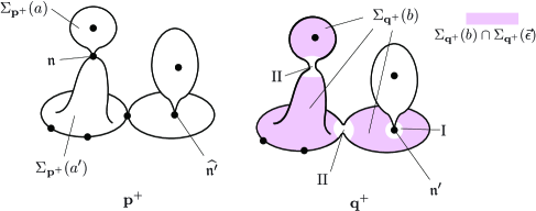
Figure 3. ${\bf p}^{+}$ and ${\bf q}^{+}$

We will define an analytic family of coordinates at a node $\mathfrak{n}^{\prime}$ in $\Sigma_{{\bf q}^{+}}(b)$. It is a family parametrized by $\mathcal{V}_{b}^{{\bf q}^{+}}$. There exists $a\in\mathcal{A}(b)$ such that $\mathfrak{n}^{\prime}$ corresponds to a nodal point $\widehat{\mathfrak{n}^{\prime}}$ of $\Sigma_{{\bf p}^{+}}$ in $\Sigma_{{\bf p}^{+}}(a)$. Then using $\varphi_{{\bf p},a,i}^{\rm s}$ or $\varphi_{{\bf p},a,i}^{\rm t}$ we can find a $\mathcal{V}_{a}^{{\bf p}^{+}}$ parametrized family of coordinates at this nodal point $\widehat{\mathfrak{n}^{\prime}}$. We regard it as a $\mathcal{V}_{b}^{{\bf q}^{+}}$ parametrized family using the identification (10.17). We thus obtain $\varphi_{{\bf q},b,i}^{\rm s}$ and $\varphi_{{\bf q},b,i}^{\rm t}$.

We next define $\phi_{{\bf r},b}$. This is a trivialization of the universal family of deformations of $\Sigma_{{\bf q}^{+}}(b)$ (equipped with marked or nodal points on it). The parameter space of this deformation is $\mathcal{V}_{b}^{{\bf r}^{+}}$. In other words if $\Sigma_{\mathfrak{v}}(b)$ together with marked points is an object corresponding to $\mathfrak{v}\in\mathcal{V}_{b}^{{\bf q}^{+}}$, the datum $\phi_{{\bf q},b}$ must be a diffeomorphism

(10.18) $$\Sigma_{{\bf q}^{+}}(b)\cong\Sigma_{\mathfrak{v}}(b).$$

Note the data $\{\phi_{{\bf p},a}\mid a\in\mathcal{A}(b)\}$ and $\{\varphi_{{\bf p},a,i}^{\rm s}\}$, $\{\varphi_{{\bf p},a,i}^{\rm t}\}$ determine a smooth embedding $\Sigma_{{\bf q}^{+}}(b)\cap\Sigma_{{\bf q}^{+}}(\vec{\epsilon})\to\Sigma_{\mathfrak{v}}(b)$ uniquely such that Diagram (10.16) commutes there. (This family of embeddings is parametrized by $\prod_{a\in\mathcal{A}(b)}\mathcal{V}_{a}^{{\bf p}^{+}}$.) We extend the family to the required family of diffeomorphisms (10.18) as follows.

We remark that $\Sigma_{{\bf q}^{+}}(b)\setminus\Sigma_{{\bf q}^{+}}(\vec{\epsilon})$ is a union of the following two kinds of connected components. (See Figure 3.)

1. A neighborhood of a nodal point of $\Sigma_{{\bf q}^{+}}$ contained in $\Sigma_{{\bf q}^{+}}(b)$.

2. A neck region in $\Sigma_{{\bf q}^{+}}(b)$. It corresponds to a nodal point of $\Sigma_{{\bf p}^{+}}$ which is resolved when we obtain $\Sigma_{{\bf q}^{+}}$ from $\Sigma_{{\bf p}^{+}}$.

To the part (I) we extend the embedding $\Sigma_{{\bf q}^{+}}(b)\cap\Sigma_{{\bf q}^{+}}(\vec{\epsilon})\to\Sigma_{\mathfrak{v}}(b)$ using the analytic families of coordinates $\varphi_{{\bf q},b,i}^{\rm s}$ or $\varphi_{{\bf q},b,i}^{\rm t}$ we produced above. In fact requiring Definition 3.7 to be satisfied makes such an extension unique.

We extend it to the part (II) in an arbitrary way. We can prove the existence of such an extension by choosing $\mathcal{V}_{b}^{{\bf q}^{+}}$ small. (The extension depends not only on the first factor but also on the second factor of (10.17).) See [FOOO4, Remark 23.5] for example for detail.

The commutativity of Diagram (10.16) is then immediate from construction. In fact if $\mathfrak{v}_{\bf q}=\left((\mathfrak{v}_{b})_{b\in\mathcal{A}_{{\bf q}}^{\rm s}\cup\mathcal{A}_{{\bf q}}^{\rm d}};(0,\dots,0),(0,\dots,0)\right)$ (namely if all the gluing parameters are $0$) then this is the way how $\phi_{{\bf q},b}$ is chosen. Then by the way how $\varphi_{{\bf q},b,i}^{\rm s}$ and $\varphi_{{\bf q},b,i}^{\rm t}$ are chosen Diagram (10.16) commutes when gluing parameters are nonzero as well. We thus proved Sublemma 10.15 and the $C^{n}$ analogue of Lemma 7.7. ∎

Remark 10.16.

In the proof of Lemma 10.13 and Sublemma 10.15 we never used the pseudo holomorphicity of $u_{\bf q}$. Therefore Lemma 10.13 and Sublemma 10.15 still hold if we replace ${\bf q}$ by ${\bf r}=((\Sigma_{\bf r},\vec{z}_{\bf r},\vec{\mathfrak{z}}_{\bf r}),u_{\bf r})$ such that $u_{\bf r}$ is smooth and ${\bf r}$ is $\epsilon$-close to ${\bf p}$.

11. Existence of obstruction bundle data

In this section we prove:

Theorem 11.1.

There exists an obstruction bundle data $\{E_{\bf p}(\bf x)\}$ of the moduli space ${\mathcal{M}}_{k+1,\ell}(X,L,J;\beta)$. We may choose it so that Condition 7.11 is satisfied.

11.1. Local construction of obstruction bundle data

Let ${\bf p}\in{\mathcal{M}}_{k+1,\ell}(X,L,J;\beta)$. We will construct an obstruction bundle data $E_{\bf q;\bf p}(\bf x)$ at ${\bf q}$ when ${\bf q}$ is in a small neighborhood of ${\bf p}$.

Lemma 11.2.

There exists a finite dimensional subspace $E^{0}_{\bf p}(\bf p)$ of $C^{\infty}(\Sigma_{\bf p},u_{\bf p}^{*}TX\otimes\Lambda^{01})$ (the set of smooth sections) such that:

1. The supports of elements of $E^{0}_{\bf p}(\bf p)$ are away from nodal points.

2. $E^{0}_{\bf p}(\bf p)$ satisfies the transversality condition in Definition 5.5.

3. $E^{0}_{\bf p}(\bf p)$ is invariant under the ${\rm Aut}^{+}({\bf p})$ action in the sense of Condition 5.6.

We may choose $E^{0}_{\bf p}(\bf p)$ so that it also satisfies Condition 7.11 and the second half of Condition 5.6 holds.

This is a standard consequence of the Fredholm property of the operator (5.5) and unique continuation. We omit the proof.

We next take a strong stabilization data $(\mathfrak{W}_{\bf p},\vec{\mathcal{N}}_{\bf p})$ as in Situation 9.8.

Let ${\bf x}\in{\mathcal{X}}_{k+1,\ell}(X,L,J;\beta)$ be $\epsilon$-close to ${\bf p}$. Using Lemma 9.9 and the definition of $\epsilon$-closeness, we can find ${}_{\bf p}\vec{\mathfrak{w}}_{\bf x}$ such that ${\bf x}\cup{}_{\bf p}\vec{\mathfrak{w}}_{\bf x}$ is $o(\epsilon)$-close to ${\bf p}\cup\vec{\mathfrak{w}}_{\bf p}$ and $u_{\bf x}({}_{\bf p}\vec{\mathfrak{w}}_{{\bf x},i})\in\mathcal{N}_{{\bf p},i}.$ Moreover the choice of such ${}_{\bf p}\vec{\mathfrak{w}}_{\bf x}$ is unique up to ${\rm Aut}({\bf x})$ action. (We also remark that ${\rm Aut}({\bf x})$ is canonically embedded to ${\rm Aut}({\bf p})$.)

Now we proceed in the same way as Subsection 8.1. We put ${\bf y}={\bf x}\cup{}_{\bf p}\vec{\mathfrak{w}}_{\bf x}$ and obtain $\mathfrak{y}$ with $\Phi_{{\bf p}^{+}}(\mathfrak{y})={\bf y}$. We then obtain the map (8.1).

(11.1) $$\mathcal{P}_{{\bf y}}:C^{2}(\Sigma_{\bf y}(\vec{\epsilon});u_{{\bf y}}^{*}TX\otimes\Lambda^{01})\to C^{2}(\Sigma_{\bf p};u_{{\bf p}}^{*}TX\otimes\Lambda^{01}).$$

Note the image of $\mathcal{P}_{{\bf y}}$ is $C^{2}(\Sigma_{\bf p}(\vec{\epsilon});u_{{\bf p}}^{*}TX\otimes\Lambda^{01})$. We may take $\vec{\epsilon}$ so that $E^{0}_{\bf p}(\bf p)$ is contained in the image of (11.1).

Definition 11.3.

We define

(11.2) $$E_{\bf p}^{0}({\bf x})=\mathcal{P}_{{\bf y}}^{-1}(E^{0}_{\bf p}(\bf p)).$$

Since the choice of ${}_{\bf p}\vec{\mathfrak{w}}_{\bf x}$ is unique up to ${\rm Aut}({\bf x})\subseteq{\rm Aut}({\bf p})$ action, Lemma 11.2 (3) implies that the right hand side of (11.2) is independent of the choice of ${}_{\bf p}\vec{\mathfrak{w}}_{\bf x}$.

We also define

(11.3) $$E_{{\bf q};{\bf p}}({\bf x})=E_{\bf p}^{0}({\bf x})$$

if ${\bf q}\in{\mathcal{M}}_{k+1,\ell}(X,L,J;\beta)$ is sufficiently close to ${\bf p}$ and ${\bf x}$ is $\epsilon$-close to ${\bf q}$.

Proposition 11.4.

If ${\bf q}$ is sufficiently close to ${\bf p}$ then $\{E_{{\bf q};{\bf p}}({\bf x})\}$ is an obstruction bundle data at ${\bf q}$.

Proof.

By Lemma 4.14, $E_{{\bf q};{\bf p}}({\bf x})$ is defined if ${\bf x}$ is $\delta$-close to ${\bf q}$ for some small $\delta$. We will check Definition 5.1 (1)(2)(3)(5). (1) is obvious from definition. (5) follows from Lemma 11.2 (3). (3) holds if ${\bf q}={\bf p}$ by Lemma 11.2 (2). Then using Mrowka’s Mayer-Vietoris principle it holds if ${\bf q}$ is sufficiently close to ${\bf p}$. See [FOOO2, Proposition 7.1.27]. We will prove (2) (smoothness of $E_{{\bf q};{\bf p}}({\bf x})$) in the next subsection.

11.2. Smoothness of obstruction bundle data

In this subsection we prove that $E_{{\bf q};{\bf p}}({\bf x})$ (which is defined in Definition 11.3) is smooth in the sense of Definition 8.7. The proof is based on Proposition 10.4.

Let ${\bf q}\in{\mathcal{M}}_{k+1,\ell}(X,L,J;\beta)$ and take stabilization and trivialization data $\mathfrak{W}_{\bf q}$. In other words (together with the strong stabilization data at ${\bf p}$ which we have taken in the last subsection), we are in Situation 10.1. We use the notations of Subsection 10.1.

We remark that the role of ${\bf p}$ in Definition 8.7 is taken by ${\bf q}$ here.

We take $\mathcal{V}({{\bf q}^{+}};\vec{\epsilon^{\prime}})$ as in (10.5) and $\overline{\mathcal{V}}({{\bf q}^{+}};\vec{\epsilon^{\prime}})=\Phi_{{\bf q^{+}}}({\mathcal{V}}({{\bf q}^{+}};\vec{\epsilon^{\prime}}))$. For $\mathfrak{y}\in\mathcal{V}({{\bf q}^{+}};\vec{\epsilon^{\prime}})$ and $u^{\prime}\in\mathscr{L}^{\bf q}_{m}$ we obtain $u^{\prime\prime}=u^{\prime}\circ\widehat{\Phi}_{{\bf q}^{+},\mathfrak{y},\vec{\epsilon^{\prime}}}^{-1}:\Sigma_{\mathfrak{y}}(\vec{\epsilon^{\prime}})\to X$ as in (10.7). We want to prove that the family of linear subspaces $\mathcal{P}_{{\bf y}}(E_{{\bf q};{\bf p}}({\bf x}))$ (see (8.7) and (8.1)) is $C^{n}$ family when we move $\mathfrak{y},u^{\prime}$. Here ${\bf x}\in\mathcal{X}_{k+1,\ell}(X,L,J;\beta)$ and ${\bf y}={\bf x}\cup{}_{\bf q}\vec{\mathfrak{w}}_{\bf x}=((\Sigma_{\mathfrak{y}},\vec{z}_{\mathfrak{y}},\vec{\mathfrak{z}}_{\mathfrak{y}}),u^{\prime\prime})$. We take ${}_{\bf p}\vec{\mathfrak{w}}_{\bf x}$ so that Condition 10.2 is satisfied. In view of Definition 11.3, we will study the composition:

(11.4) $$\mathcal{P}_{{\bf x}\cup{}_{\bf q}\vec{\mathfrak{w}}_{\bf x}} \circ\mathcal{P}_{{\bf x}\cup{}_{\bf p}\vec{\mathfrak{w}}_{\bf x}}^{-1}:C^{\infty}(\Sigma_{{\bf p}^{+}}(\vec{\epsilon});u_{{\bf p}}^{*}TX\otimes\Lambda^{01})$$

$$\to L^{2}_{m}(\Sigma_{\mathfrak{y}}(\vec{\epsilon^{\prime}});u_{{\bf x}}^{*}TX\otimes\Lambda^{01})\to L^{2}_{m}(\Sigma_{{\bf q}^{+}}(\vec{\epsilon^{\prime}});u_{{\bf q}}^{*}TX\otimes\Lambda^{01})$$

and study $C^{n}$ dependence of the image of $E^{0}_{\bf p}({\bf p})$ by this map.

Remark 11.5.

Note when we define $\mathcal{P}_{{\bf x}\cup{}_{\bf q}\vec{\mathfrak{w}}_{\bf x}}$ we take $\bf q$ and ${\bf x}\cup{}_{\bf q}\vec{\mathfrak{w}}_{\bf x}$ in place of $\bf p$ and ${\bf y}$ in (8.1). When we define $\mathcal{P}_{{\bf x}\cup{}_{\bf p}\vec{\mathfrak{w}}_{\bf x}}$ we take $\bf p$ and ${\bf x}\cup{}_{\bf p}\vec{\mathfrak{w}}_{\bf x}$ in place of $\bf p$ and ${\bf y}$ in (8.1).

We remark that Definition 8.5 (1)(2) and Definition 8.7 (1) is obvious from construction. To prove Definition 8.5 (3) (and so Definition 8.7 (2)) it suffices to prove the next lemma .

Lemma 11.6.

If ${\bf e}\in C^{\infty}(\Sigma_{\bf p};u_{{\bf p}}^{*}TX\otimes\Lambda^{01})$ is a smooth section which has a small compact support in $\Sigma_{{\bf p}^{+}}(\vec{\epsilon})$, then the map $({\mathfrak{y}},u^{\prime})\mapsto(\mathcal{P}_{{\bf x}\cup{}_{\bf q}\vec{\mathfrak{w}}_{\bf x}}\circ\mathcal{P}_{{\bf x}\cup{}_{\bf p}\vec{\mathfrak{w}}_{\bf x}}^{-1})({\bf e})$ is a $C^{n-1}$ map to $L^{2}_{m}(\Sigma_{\bf q}(\vec{\epsilon^{\prime}});u_{{\bf q}}^{*}TX\otimes\Lambda^{01})$.

Proof.

Let $U^{\bf p}$ be a support of ${\bf e}$ and $z^{\bf p}$ its coordinate. Let $\Psi_{{\bf p},{\bf q}}$ be as in Definition 10.3. We may assume $\Psi_{{\bf p},{\bf q}}(\overline{\mathcal{V}}({{\bf q}^{+}};\vec{\epsilon^{\prime}})\times\mathscr{L}^{\bf q}_{m}\times U^{\bf p})$ is contained in a single chart $U^{\bf q}$ and let $z^{\bf q}$ be its coordinate.

We may also assume that $u^{\prime}(U^{\bf q})$ for any $u^{\prime}\in\mathscr{L}^{\bf q}_{m}$ and $u_{\bf p}(U^{\bf p})$ are contained in a single chart $U^{X}$ of $X$ and denote by ${\mathfrak{e}}_{1},\dots,{\mathfrak{e}}_{d}$, sections of the complex vector bundle $TX$ on $U^{X}$ which give a basis at all points.

We put $\mathfrak{a}=\Phi_{{\bf q}^{+}}(\mathfrak{y})\in\overline{\mathcal{V}}({{\bf q}^{+}};\vec{\epsilon^{\prime}})$. During the calculation below we write $\Psi_{{\bf p},{\bf q}}(z)=\Psi_{{\bf p},{\bf q}}(\mathfrak{a},u^{\prime},z)$ for simplicity. By definition the map $\mathcal{P}_{{\bf x}\cup{}_{\bf q}\vec{\mathfrak{w}}_{\bf x}}\circ\mathcal{P}_{{\bf x}\cup{}_{\bf p}\vec{\mathfrak{w}}_{\bf x}}^{-1}$ is induced by a bundle map which is the tensor product of two bundle maps. One of them (See (8.2)) is a composition of the parallel transports

(11.5) $$T_{u_{\bf p}(\Psi_{{\bf p},{\bf q}}^{-1}(z^{\bf q}))}X\longrightarrow T_{u^{\prime}(z^{\bf q})}X\longrightarrow T_{u_{\bf q}(z^{\bf q})}X.$$

The other is (See (8.3).)

(11.6) $$\Lambda^{01}_{\Psi_{{\bf p},{\bf q}}^{-1}(z^{\bf q})}\Sigma_{\bf p}\longrightarrow\Lambda^{01}_{\hat{\Phi}_{{\bf q}^{+},\mathfrak{y},\vec{\epsilon^{\prime}}}(z^{\bf q})}\Sigma_{\bf x}\longrightarrow\Lambda^{01}_{z^{\bf q}}\Sigma_{\bf q}.$$

The arrows in (11.6) are the complex linear parts of the derivatives of $\widehat{\Phi}_{{\bf q}^{+},\mathfrak{y},\vec{\epsilon^{\prime}}}\circ\Psi_{{\bf p},{\bf q}}$ and of $\hat{\Phi}_{{\bf q}^{+},\mathfrak{y},\vec{\epsilon^{\prime}}}^{-1}$. In fact, by Definition 10.3 and (10.4), $\widehat{\Phi}_{{\bf q}^{+},\mathfrak{y},\vec{\epsilon^{\prime}}}\circ\Psi_{{\bf p},{\bf q}}=\widehat{\Phi}_{{\bf p}^{+},\mathfrak{x}_{\bf p},\vec{\epsilon}}$, where $\mathfrak{x}_{\bf p}$ is defined by ${\bf x}\cup{}_{\bf p}\vec{\mathfrak{w}}_{\bf x}={\Phi}_{{\bf p}^{+}}(\mathfrak{x}_{\bf p})$.

If $h=\sum_{i}h_{i}\mathfrak{e}_{i}$ is a section of $u_{\bf p}^{*}TX$ on $U^{\bf p}$ then (11.5) sends $h$ to the section

$$z^{\bf q}\mapsto\sum_{i,j}h_{i}(\Psi_{{\bf p},{\bf q}}(\mathfrak{a},u^{\prime},z^{\bf q}))G_{ij}(u_{\bf q}(z^{\bf q}),u^{\prime}(z^{\bf q}),u_{\bf p}(\Psi_{{\bf p},{\bf q}}(\mathfrak{a},u^{\prime},z^{\bf q})))\mathfrak{e}_{j}$$

Here $G_{ij}$ is a smooth function on $U^{X}\times U^{X}\times U^{X}$.

We take a $\mathfrak{y}$ parametrized (smooth) family of complex structures $j_{\mathfrak{y}}$ on $U^{\bf q}$, which is a pull back of the complex structure on $\Sigma_{\bf x}=\Sigma_{\mathfrak{y}}$ by $\widehat{\Phi}_{{\bf q}^{+},\mathfrak{y},\vec{\epsilon^{\prime}}}$. Then (11.6) is a composition of

$$(D\Psi_{{\bf p},{\bf q}})^{01}:\Lambda^{01}_{\Psi_{{\bf p},{\bf q}}^{-1}(z^{\bf q})}U^{\bf p}\to\Lambda^{01}_{z^{\bf q}}(U^{\bf q},j_{\mathfrak{y}})\quad\text{and}\quad({\rm id})^{01}:\Lambda^{01}_{z^{\bf q}}(U^{\bf q},j_{\mathfrak{y}})\to\Lambda^{01}_{z^{\bf q}}(U^{\bf q},j_{0}).$$

(Here $j_{0}$ is the complex structure of $U^{\bf q}\subset\Sigma_{\bf q}$.) Therefore using Proposition 10.4 there exists a $C^{n-1}$ function $f(\mathfrak{y},u^{\prime},z^{\bf q})$ such that (11.6) is written as

$$d\overline{z}^{\bf p}\mapsto f(\mathfrak{y},u^{\prime},z^{\bf q})d\overline{z}^{\bf q}.$$

We put ${\bf e}=\sum_{i}{\bf e}_{i}(z^{\bf p})\mathfrak{e}_{i}\otimes d\overline{z}^{\bf p}$. Here ${\bf e}_{i}$ are smooth functions. Then

$$(\mathcal{P}_{{\bf x}\cup{}_{\bf q}\vec{\mathfrak{w}}_{\bf x}}\circ\mathcal{P}_{{\bf x}\cup{}_{\bf p}\vec{\mathfrak{w}}_{\bf x}}^{-1})({\bf e})$$

$$=f(\mathfrak{y},u^{\prime},z^{\bf q})\sum_{i,j}{\bf e}_{i}(\Psi_{{\bf p},{\bf q}}(\mathfrak{a},u^{\prime},z^{\bf q}))G_{ij}(u_{\bf q}(z^{\bf q}),u^{\prime}(z^{\bf q}),u_{\bf p}(\Psi_{{\bf p},{\bf q}}(\mathfrak{a},u^{\prime},z^{\bf q})))\mathfrak{e}_{j}\otimes d\overline{z}^{\bf q}.$$

Since ${\bf e}_{i}$, $u_{\bf p}$, $u_{\bf q}$, $G_{ij}$ are smooth, $f$ is of $C^{n-1}$ class, $\Psi_{{\bf p},{\bf q}}$ is of $C^{n}$ class, and $\mathfrak{a}=\Phi_{{\bf q}^{+}}(\mathfrak{y})$ with $\Phi_{{\bf q}^{+}}$ smooth, this is a $C^{n-1}$ map of $(\mathfrak{y},u^{\prime},z^{\bf q})$, as required. ∎

Definition 8.7 (2) is now proved. We remark that we never used the fact that $u_{\bf q}$ is pseudo holomorphic in the above proof. Therefore the proof of Definition 8.7 (3) is the same. The proof of Proposition 11.4 is complete. ∎

11.3. Global construction of obstruction bundle data

In this and the next subsections we prove Theorem 11.1. The proof is based on the argument of [FOn, page 1003-1004]. For each ${\bf p}\in\mathcal{M}_{k+1,\ell}(X,L;\beta)$ we use Proposition 11.4 to find its neighborhood $\mathfrak{U}({\bf p})$ in $\mathcal{M}_{k+1,\ell}(X,L;\beta)$ such that if ${\bf q}\in\mathfrak{U}({\bf p})$ then $E_{{\bf q};{\bf p}}({\bf x})$ is an obstruction bundle data at ${\bf q}$. We take a compact subset $K(\bf p)$ of $\mathfrak{U}({\bf p})$ such that $K({\bf p})$ is the closure of an open neighborhood $K_{o}({\bf p})$ of ${\bf p}$.

We note that during the construction of $E_{{\bf q};{\bf p}}({\bf x})$ we have chosen a linear subspace $E^{0}_{\bf p}(\bf p)$ (See Lemma 11.2.) as well as strong stabilization data at ${\bf p}$.

Since $\mathcal{M}_{k+1,\ell}(X,L;\beta)$ is compact, we can find a finite subset $\{{\bf p}_{1},\dots,{\bf p}_{\mathscr{P}}\}$ of $\mathcal{M}_{k+1,\ell}(X,L;\beta)$ such that

(11.7) $$\bigcup_{i=1}^{\mathscr{P}}K_{o}({\bf p}_{i})=\mathcal{M}_{k+1,\ell}(X,L;\beta).$$

For ${\bf q}\in\mathcal{M}_{k+1,\ell}(X,L;\beta)$ we put $I({\bf q})=\{i\in\{1,\dots,\mathscr{P}\}\mid{\bf q}\in K({\bf p}_{i})\}.$

Lemma 11.7.

We may perturb $E^{0}_{{\bf p}_{i}}({\bf p}_{i})$ by an arbitrary small amount in $C^{2}$ norm so that the following holds. For each ${\bf q}\in\mathcal{M}_{k+1,\ell}(X,L;\beta)$ the sum $\sum_{i\in I({\bf q})}E_{{\bf q},{\bf p}_{i}}({\bf q})$ of vector subspaces in $C^{\infty}(\Sigma_{\bf q}(\vec{\epsilon^{\prime}});u_{{\bf q}}^{*}TX\otimes\Lambda^{01})$ is a direct sum

(11.8) $$\bigoplus_{i\in I({\bf q})}E_{{\bf q},{\bf p}_{i}}({\bf q}).$$

Postponing the proof of Lemma 11.7 to the next subsection we continue the proof of Theorem 11.1.

Note we may choose $E^{\prime,0}_{{\bf p}_{i}}$, the perturbation of $E^{0}_{{\bf p}_{i}}$, sufficiently close to $E^{0}_{{\bf p}_{i}}$, so that for ${\bf q}\in K({\bf p}_{i})$ the conclusion of Proposition 11.4 still holds after this perturbation.

For each ${\bf x}$ sufficiently close to ${\bf q}$ we define $E_{\bf q}({\bf x})=\bigoplus_{i\in I({\bf q})}E_{{\bf q},{\bf p}_{i}}({\bf x}).$ (Since ${\bf x}$ is sufficiently close to ${\bf q}$ the right hand side is still a direct sum by Lemma 11.7.)

Now we prove that $\{E_{\bf q}({\bf x})\}$ satisfies Definition 5.1 (1)-(5). (1)(2)(5) are immediate consequences of the fact that $E_{{\bf q},{\bf p}_{i}}({\bf x})$ satisfies the same property. (3) is a consequence of $I(\bf q)\neq\emptyset$ (which follows from (11.7)) and the fact that $E_{{\bf q},{\bf p}_{i}}({\bf x})$ satisfies (3).

We check (4). Let ${\bf q}\in\mathcal{M}_{k+1,\ell}(X,L;\beta)$. Since $K({\bf p}_{i})$ are all closed sets, there exists a neighborhood $U(\bf q)$ in $\mathcal{M}_{k+1,\ell}(X,L;\beta)$ such that ${\bf q}^{\prime}\in U(\bf q)$ implies $I({\bf q}^{\prime})\subseteq I({\bf q})$. Therefore $E_{{\bf q}^{\prime}}({\bf x})\subseteq E_{\bf q}({\bf x})$ when both sides are defined. This implies (4).

11.4. Proof of Lemma 11.7

To complete the proof of Theorem 11.1 it remains to prove Lemma 11.7. The proof here is a copy of [FOOO4, Section 27]. We begin with two simple lemmas. (All the vector spaces in this subsection are complex vector spaces.)

Situation 11.8.

Let $V$ be a $D$ dimensional manifold, $V_{i}$ ($i=1,\dots,l$) open subsets of $V$ and $K_{i}\subset V_{i}$ compact subsets. $\pi_{i}:\mathcal{E}_{i}\to V_{i}$ is a $d_{i}$ dimensional vector bundle on $V_{i}$ and $E$ is a $d$ dimensional vector space. Suppose $F_{i}:\mathcal{E}_{i}\to E$ is a $C^{1}$ map which is linear on each fiber of $\mathcal{E}_{i}$. Let $Gr_{a}(E)$ be the Grassmannian manifold consisting of all $a$ dimensional subspaces of $E$.

Lemma 11.9.

In Situation 11.8 we assume

(11.9) $$a+D\sum d_{i}<d.$$

Then the set of $E_{0}\in Gr_{a}(E)$ satisfying the next condition is dense.

1. For any $v\in V$ we consider the sum of the linear subspaces $F_{i}(\pi_{i}^{-1}(v))\subset E$ for $i$ with $v\in K_{i}$ and denote it by $F(v)$. Then

   $$F(v)\cap E_{0}=\{0\}.$$

Proof.

The proof is by induction on $a$. Suppose $E^{\prime}_{0}\in Gr_{a-1}(E)$ satisfies (*). It suffices to prove that the set of $e\in E\setminus\{0\}$ such that ${\mathbb{C}}e\cap E^{\prime}_{0}=\{0\}$ and $E^{\prime}_{0}+{\mathbb{C}}e$ satisfies (*) is dense.

Let $\mathcal{L}\subset\{1,\dots,l\}$ and $U_{\mathcal{L}}=\bigcap_{i\in\mathcal{L}}U_{i}$. Let $\mathcal{E}_{\mathcal{L}}$ be the total space of the Whitney sum bundle $\bigoplus_{i\in\mathcal{L}}\mathcal{E}_{i}$ on $U_{\mathcal{L}}$. We define $\hat{F}_{\mathcal{L}}:{\mathbb{C}}\times E^{\prime}_{0}\times\mathcal{E}_{\mathcal{L}}\to E$ as follows. Let $w_{i}\in\pi_{i}^{-1}(v)\subset\mathcal{E}_{i}$, then

$$\hat{F}_{\mathcal{L}}(r,x,(w_{i})_{i\in\mathcal{L}})=r(x+\sum_{i\in\mathcal{L}}F_{i}(w_{i})).$$

This map is $C^{1}$ and the dimension of the domain is strictly smaller than $d$. Therefore the image of $\hat{F}_{\mathcal{L}}$ is nowhere dense. On the other hand if $e$ is not contained in the union of the images of $\hat{F}_{\mathcal{L}}$ for various $\mathcal{L}$, then $E^{\prime}_{0}+{\mathbb{C}}e$ satisfies (*). In fact suppose $\sum F_{i}(w_{i})+v+ce=0$ with $w_{i}\in\pi_{i}^{-1}(v)$, $v\in E$ and $c\in{\mathbb{C}}$. If $c=0$ the induction hypothesis implies $\sum_{i}F_{i}(w_{i})=0$, $v=0$. If $c\neq 0$, then $e=\hat{F}_{\mathcal{L}}(-1/c,v,(w_{i}))$, a contradiction. ∎

We use the equivariant version of Lemma 11.9.

Situation 11.10.

Let $\Gamma$ be a finite group of order $g$ and $d^{\prime}>0$. In Situation 11.8 we assume in addition that $E$ is a $\Gamma$ vector space such that any irreducible representation $W_{\sigma}$ of $\Gamma$ has its multiplicity in $E$ larger than $d^{\prime}$. Let ${\rm Rep}(\Gamma)$ be the set of all irreducible representations of $\Gamma$ over ${\mathbb{C}}$.

Let $Gr_{(a_{\sigma}:\sigma\in{\rm Rep}(\Gamma))}(E)$ be the set of all $\Gamma$ invariant linear subspaces $E_{0}$ of $E$ such that $E_{0}$ is isomorphic to $\bigoplus_{\sigma\in{\rm Rep}(\Gamma)}W_{\sigma}^{a_{\sigma}}$ as $\Gamma$ vector spaces. Let $a=\sup\{a_{\sigma}\}$.

Lemma 11.11.

Suppose we are in Situation 11.10. We assume

(11.10) $$a+gD\sum d_{i}<d^{\prime}.$$

Then the set of all $E_{0}\in Gr_{(a_{\sigma}:\sigma\in{\rm Rep}(\Gamma))}(E)$ satisfying the Condition (*) in Lemma 11.9 is dense in $Gr_{(a_{\sigma}:\sigma\in{\rm Rep}(\Gamma))}(E)$.

Note we do not assume $\Gamma$ equivariance of $V$, $\mathcal{E}_{i}$ or $F_{i}$ in Lemma 11.11.

Proof.

Let $m_{\sigma}\geq d^{\prime}$ be the multiplicity of $W_{\sigma}$ in $E$. Then there exists an obvious diffeomorphism

(11.11) $$Gr_{(a_{\sigma}:\sigma\in{\rm Rep}(\Gamma))}(E)\cong\prod_{\sigma}Gr_{a_{\sigma},m_{\sigma}}.$$

Here $Gr_{a_{\sigma},m_{\sigma}}$ is the Grassmanian manifold of all $a_{\sigma}$ dimensional subspace of ${\mathbb{C}}^{m_{\sigma}}$. Let ${\mathbb{C}}[\Gamma]$ be the group ring of the finite group $\Gamma$. We put:

(11.12) $$\mathcal{E}^{+}_{i}=\mathcal{E}_{i}\otimes_{{\mathbb{C}}}{\mathbb{C}}[\Gamma]\cong\bigoplus_{\sigma\in{\rm Rep}(\Gamma)}\mathcal{E}_{i}\otimes_{{\mathbb{C}}}W_{\sigma}^{d_{\sigma}}.$$

Here $d_{\sigma}$ is the multiplicity of $W_{\sigma}$ in ${\mathbb{C}}[\Gamma]$. Note $d_{\sigma}\leq g$. (11.12) is an isomorphism of $\Gamma$ equivariant vector bundles. $F_{i}$ induces a $\Gamma$ equivariant map $\mathcal{E}^{+}_{i}\to E_{0}$. It then induces $\Gamma$ equivariant fiberwise linear maps $F_{i,\sigma}:\mathcal{E}_{i}\otimes_{{\mathbb{C}}}W_{\sigma}^{d_{\sigma}}\to W_{\sigma}^{m_{\sigma}}$ by decomposing into irreducible representations. The map $F_{i,\sigma}$ can be identified with a fiberwise ${\mathbb{C}}$-linear map $\overline{F}_{i,\sigma}:\mathcal{E}_{i}\otimes_{{\mathbb{C}}}{\mathbb{C}}^{d_{\sigma}}\to{\mathbb{C}}^{m_{\sigma}}$ by Schur’s lemma. (11.10) implies $a_{\sigma}+Dd_{\sigma}\sum d_{i}<m_{\sigma}.$ Therefore using (11.11) we apply Lemma 11.9 for each $\sigma$ and prove Lemma 11.11. ∎

Proof of Lemma 11.7.

We take $\{{\bf p}_{1},\dots,{\bf p}_{\mathscr{P}}\}$, $\mathfrak{U}({\bf p}_{i})$, $K({\bf p}_{i})$ as in Subsection 11.3. We also have taken $E^{0}_{{\bf p}_{i}}({\bf p}_{i})$ so that the conclusion of Lemma 11.2 is satisfied. Let $\mathfrak{d}$ be the supremum of the dimension of $E^{0}_{{\bf p}_{i}}({\bf p}_{i})$ and $g$ the supremum of the order of ${\rm Aut}^{+}({\bf p}_{i})$. For each $i$ we take $E^{+}({\bf p}_{i})$ in $C^{\infty}(\Sigma_{{\bf p}_{i}},u_{{\bf p}_{i}}^{*}TX\otimes\Lambda^{01})$ such that:

1. Lemma 11.2 (1)(3) are satisfied.

2. $E^{0}_{{\bf p}_{i}}({\bf p}_{i})\subset E^{+}({\bf p}_{i})$.

3. For any irreducible representation $W_{\sigma}$ of ${\rm Aut}^{+}({\bf p}_{i})$ the multiplicity of $W_{\sigma}$ in $E^{+}({\bf p}_{i})$ is larger than $d^{+}$. Here $d^{+}$ is determined later.

We will prove, by induction on $I=1,\dots,\mathscr{P}$, that we can perturb $E^{0}_{{\bf p}_{i}}({\bf p}_{i})$ in $E^{+}({\bf p}_{i})$ in an arbitrary small amount to obtain $E^{1}_{{\bf p}_{i}}({\bf p}_{i})$ so that statement ($I$) holds.

1. For any $J\subseteq\{1,\dots,I\}$ and ${\bf q}\in\bigcap_{i\in J}K({\bf p}_{i})$, the sum $\sum_{i\in J}E^{\prime}_{{\bf q};{\bf p}_{i}}({\bf q})$ is a direct sum. Here we define $E^{\prime}_{{\bf q};{\bf p}_{i}}({\bf q})$ in the same way as $E_{{\bf q};{\bf p}_{i}}({\bf q})$, using $E^{1}_{{\bf p}_{i}}({\bf p}_{i})$ instead of $E^{0}_{{\bf p}_{i}}({\bf p}_{i})$.

Suppose ($I-1$) holds. We choose a weak stabilization data $\vec{\mathfrak{w}}_{{\bf p}_{I}}$ and a neighborhood $\mathscr{N}({\bf p}^{+}_{I})\subset\mathcal{X}_{k+1,\ell+\ell^{\prime}}(X,L;\beta)$ of ${\bf p}^{+}_{I}={\bf p}_{I}\cup\vec{\mathfrak{w}}_{{\bf p}_{I}}$. We define obstruction bundle data $\{E_{{\bf p}_{I}}({\bf x})\}$ at ${\bf p}_{I}$ by using $E^{0}_{{\bf p}_{I}}({\bf p}_{I})$. Proposition 11.4 and Lemma 9.11 then imply that

$$U({\bf p}^{+}_{I}):=\{{\bf x}\in\mathscr{N}({\bf p}^{+}_{I})\mid\overline{\partial}u_{\bf x}\in E_{{\bf p}_{I}}({\bf x})\}$$

has a structure of a finite dimensional orbifold $V({\bf p}^{+}_{I})/{\rm Aut}({\bf p}^{+}_{I})$. Let $D$ be the supremum of the dimension of $V({\bf p}^{+}_{I})$ for $I=1,\dots,\mathscr{P}$.

We apply Lemma 11.11 as follows. Put $V=V({\bf p}^{+}_{I})$, $E=E^{+}({\bf p}_{I})$, $\Gamma={\rm Aut}({\bf p}^{+}_{I})$. For $i\leq I-1$, we define $K_{i}$ as the inverse image of $K_{{\bf p}_{i}}\cap K_{{\bf p}_{I}}\cap U({\bf p}^{+}_{I})$ in $V({\bf p}^{+}_{I})$ and take a sufficiently small neighborhood $V_{i}$ of $K_{i}$. For $\tilde{\bf y}\in V_{i}$ we take its image ${\bf y}\in U({\bf p}^{+}_{I})$. Put $\mathcal{E}_{i}(\tilde{\bf y})=E^{1}_{{\bf p}_{i}}(\mathfrak{forget}_{\ell+\ell^{\prime},\ell}({\bf y}))$ and define a vector bundle $\mathcal{E}_{i}=\bigcup_{\tilde{\bf y}\in V_{i}}\mathcal{E}_{i}(\tilde{\bf y})\times\{\tilde{\bf y}\}$ on $V_{i}$. We consider an isomorphism

$$\mathcal{P}_{{\bf y}}:L^{2}_{m}(\Sigma_{\bf y}(\vec{\epsilon});u_{{\bf y}}^{*}TX\otimes\Lambda^{01})\to L^{2}_{m}(\Sigma_{{\bf p}_{I}}(\vec{\epsilon});u_{{\bf p}_{I}}^{*}TX\otimes\Lambda^{01})$$

for $\tilde{\bf y}\in V_{i}$ with ${\bf y}=[\tilde{\bf y}]\in U({\bf p}^{+}_{I})$ and compose $\mathcal{P}_{{\bf y}}$ with the orthogonal projection $\Pi:L^{2}_{m}(\Sigma_{{\bf p}_{I}}(\vec{\epsilon});u_{{\bf p}_{I}}^{*}TX\otimes\Lambda^{01})\to E^{+}({\bf p}_{I})=E$. The restrictions to $\mathcal{E}_{i}(\tilde{\bf y})$ of the composition $\Pi\circ\mathcal{P}_{{\bf y}}$ for various $\tilde{\bf y}\in V_{i}$ defines a $C^{1}$ map $F_{i}:\mathcal{E}_{i}\to E$.

We may take $d^{+}$ depending only on $\mathscr{P}$, $g$, $\mathfrak{d}$, $D$ so that (11.10) is satisfied. By Lemma 11.11, we obtain $(I)$ as an immediate consequence of $(I-1)$ and Lemma 11.9 $(*)$.

The claim $(I)$, in the case $I=\mathscr{P}$, implies Lemma 11.7. ∎

12. From $C^{n}$ to $C^{\infty}$

In Sections 9 and 10 we have constructed a Kuranishi structure of $C^{n}$ class for arbitrary but fixed $n$. In this section we provide the way to construct one of $C^{\infty}$ class. The argument of this section is a copy of [FOOO4, Section 26]. We use Condition (3) in Definition 8.7 in this section.

12.1. $C^{\infty}$ structure of Kuranishi chart

We study the map $({\rm Pr}^{\rm source},{\rm Pr}^{\rm map})$ and also $V_{\bf p}\subset U_{{\bf p}^{+}}$. ($U_{{\bf p}^{+}}$ is defined in Definition 7.2. $V_{\bf p}$ is defined in Definition 9.10.) In Section 9 we proved that the image of $U_{{\bf p}^{+}}$ by the map $({\rm Pr}^{\rm source},{\rm Pr}^{\rm map})$ is a $C^{n}$ submanifold if $m$ is sufficiently larger than $n$ and also the image of $V_{\bf p}$ is a $C^{n}$ submanifold. We first remark the following:

Lemma 12.1.

The images of $U_{{\bf p}^{+}}$ and $V_{\bf p}$ by the map $({\rm Pr}^{\rm source},{\rm Pr}^{\rm map})$ are $C^{\infty}$ submanifolds at ${\bf p}^{+}$.

Proof.

It suffices to show that they are of $C^{n^{\prime}}$ class for any $n^{\prime}$. It is obvious from the construction of Subsection 10.3 that for any $n^{\prime}$ we can find $m^{\prime}$ such that for an open neighborhood $U^{\prime}_{{\bf p}^{+}}$ of ${\bf p}^{+}$ in $U_{{\bf p}^{+}}$ and $\vec{\epsilon^{\prime}}$ the next diagram commutes.

(12.1) $$\begin{CD}U^{\prime}_{{\bf p}^{+}}@ >{({\rm Pr}^{\rm source},{\rm Pr}^{\rm map})}>>\!\!\!\!\!\!\!\!\!\!\!\!\!\!\!\!\!\!\!\!\!\!\!\!\!\!\!\!\!\!\!\!\!\!\!\!\!\!\!\!\!\!\!\!\!\!\!\!\!\!\!\!\!\!\!\!\!\!\!\!\!\!\mathcal{M}^{\rm d,log}_{k+1,\ell+\ell^{\prime}}\atop\times L^{2}_{m^{\prime}}(\Sigma_{{\bf p}\cup\vec{\mathfrak{w}}_{\bf p}}(\vec{\epsilon^{\prime}}),\partial\Sigma_{{\bf p}\cup\vec{\mathfrak{w}}_{\bf p}}(\vec{\epsilon^{\prime}});X,L)\\ @ VVV@V{}V{}V\\ U_{{\bf p}^{+}}@ >{({\rm Pr}^{\rm source},{\rm Pr}^{\rm map})}>>\!\!\!\!\!\!\!\!\!\!\!\!\!\!\!\!\!\!\!\!\!\!\!\!\!\!\!\!\!\!\!\!\!\!\!\!\!\!\!\!\!\!\!\!\!\!\!\!\!\!\!\!\!\!\!\!\!\!\!\!\!\!\mathcal{M}^{\rm d,log}_{k+1,\ell+\ell^{\prime}}\atop\times L^{2}_{m}(\Sigma_{{\bf p}\cup\vec{\mathfrak{w}}_{\bf p}}(\vec{\epsilon}),\partial\Sigma_{{\bf p}\cup\vec{\mathfrak{w}}_{\bf p}}(\vec{\epsilon});X,L)\end{CD}$$

where vertical arrows are inclusions. Moreover the first horizontal arrow is of $C^{n^{\prime}}$ class and the image of $V_{\bf p}$ by the first horizontal arrow is also of $C^{n^{\prime}}$ class. (See Lemma 10.10.) Therefore the image of the second horizontal arrow is of $C^{n^{\prime}}$ class at the image of ${\bf p}^{+}$ and that the image of $V_{\bf p}$ by the second horizontal arrow is also of $C^{n^{\prime}}$ class at the image of ${\bf p}^{+}$. The lemma follows. ∎

Note the size of the neighborhood $U^{\prime}_{{\bf p}^{+}}$ may become smaller and converge to $0$ as $m^{\prime}$ goes to infinity. So the above proof of Lemma 12.1 can be used to show the smoothness of $U_{{\bf p}^{+}}$ and $V_{\bf p}$ only at ${\bf p}^{+}$. We fix $m$, $U_{\bf p}^{+}$ and $V_{\bf p}$ and will prove:

Proposition 12.2.

The image of $V_{\bf p}$ by the map $({\rm Pr}^{\rm source},{\rm Pr}^{\rm map})$ is a submanifold of $C^{\infty}$ class.

Corollary 12.3.

The Kuranishi chart $(U_{\bf p},\mathcal{E}_{\bf p},\mathfrak{s}_{\bf p},\psi_{\bf p})$ we produced in Section 9 is of $C^{\infty}$ class.

It is easy to see that Proposition 12.2 implies Corollary 12.3.

Proof of Proposition 12.2.

Let ${\bf r}^{+}\in V_{\bf p}\subset U_{{\bf p}^{+}}$. We put ${\bf r}^{+}={\bf r}\cup\vec{\mathfrak{w}}_{\bf r}$ where ${\bf r}=((\Sigma_{\bf r},\vec{z}_{\bf r},\vec{\mathfrak{z}}_{\bf r}),u_{\bf r}).$ We apply Lemma 10.13 with ${\bf q}$ replaced by ${\bf r}$ (See Remark 10.16.) and obtain $\mathfrak{W}_{\bf r}=(\vec{\mathfrak{w}}_{\bf r},\{\varphi_{{\bf r},a,i}^{\rm s}\},\{\varphi_{{\bf r},a,j}^{\rm d}\},\{\psi_{{\bf r},a}\})$. (See Remark 8.6.)

We write ${\rm Pr}^{\rm map}_{\bf p}$ etc. in place of ${\rm Pr}^{\rm map}$ hereafter. We recall that the map ${\rm Pr}^{\rm map}_{\bf p}$ (resp. ${\rm Pr}^{\rm map}_{\bf r}$) depends not only on the weak stabilization data $\vec{\mathfrak{w}}_{\bf p}$ (resp. $\vec{\mathfrak{w}}_{\bf r}$) but also on the stabilization and trivialization data, $\mathfrak{W}_{\bf p}=(\vec{\mathfrak{w}}_{\bf p},\{\varphi_{{\bf p},a,i}^{\rm s}\},\{\varphi_{{\bf p},a,j}^{\rm d}\},\{\phi_{{\bf p},a}\})$ (resp. $\mathfrak{W}_{\bf r}=(\vec{\mathfrak{w}}_{\bf r},\{\varphi_{{\bf r},a,i}^{\rm s}\},\{\varphi_{{\bf r},a,j}^{\rm d}\},\{\psi_{{\bf r},a}\})$).

We consider Diagram (10.14) with ${\bf q}$ replaced by ${\bf r}$. For each $n^{\prime}$ we can choose $m^{\prime}$ such that the image of the first horizontal arrow is of $C^{n^{\prime}}$ class. (Here we use Definition 8.7 (3) for ${\bf r}$ and apply the $C^{n^{\prime}}$ version of Lemma 7.3 (which is proved in Subsection 9.4) at ${\bf r}$.) The right vertical arrow is smooth. In fact this map is $f\mapsto f\circ\phi$ for an open smooth embedding $\phi$ mentioned in Lemma 10.13.

Therefore the commutativity of Diagram (10.14) implies that the image of $({\rm Pr}^{\rm source},{\rm Pr}^{\rm map}_{\bf p})$ in Diagram (10.14) is of $C^{n^{\prime}}$ class at ${\bf r}^{+}$. We can also prove that the image of $V_{\bf p}$ under the map $({\rm Pr}^{\rm source},{\rm Pr}^{\rm map}_{\bf p})$ is of $C^{n^{\prime}}$ class at ${\bf r}^{+}$. Since $n^{\prime}$ and ${\bf r}^{+}$ are arbitrary, Proposition 12.2 follows. The proof of Proposition 12.2 and Lemma 7.3 (the $C^{\infty}$ version) are now complete. ∎

12.2. Smoothness of coordinate change

In this subsection we prove that the coordinate change we produced in Section 10 is of $C^{\infty}$ class with respect to the $C^{\infty}$ structure we defined in the last subsection.

We first consider the case ${\bf q}={\bf p}$. We take two strong stabilization data $(\mathfrak{W}_{\bf p}^{j},\vec{\mathcal{N}}_{\bf p}^{j})$ $(j=1,2)$ at ${\bf p}$. Moreover we take two obstruction bundle data $\{E_{\bf p}^{j}(\bf x)\}$ $(j=1,2)$ at ${\bf p}$. We obtain two Kuranishi charts $(U^{j}_{\bf p},\mathcal{E}^{j}_{\bf p},\mathfrak{s}^{j}_{\bf p},\psi^{j}_{\bf p})$ for $j=1,2$ using them. We assume $E_{\bf p}^{1}({\bf x})\subseteq E_{{\bf p}}^{2}({\bf x})$.

Then by the construction of Subsection 7.3 we obtain a coordinate change $(\varphi_{21},\hat{\varphi}_{21})$, where $\varphi_{21}:U^{21}_{\bf p}\to U^{2}_{\bf p}$ is an embedding of orbifolds from open subset $U^{21}_{\bf p}$ of $U^{1}_{\bf p}$. The map $\hat{\varphi}_{21}$ is an embedding of orbibundles $\mathcal{E}^{1}_{\bf p}|_{U^{21}_{\bf p}}\to\mathcal{E}^{2}_{\bf p}$.

Lemma 12.4.

$\varphi_{21}$, $\hat{\varphi}_{21}$ are of $C^{\infty}$ class at ${\bf p}$.

Proof.

The proof is similar to the proof of Lemma 12.1. For any $n^{\prime}$ we can use $L^{2}_{m^{\prime}}$ space to show that $\varphi_{21}$, $\hat{\varphi}_{21}$ are of $C^{n^{\prime}}$ class on $U^{21}_{\bf p}\cap U^{\prime}_{\bf p}$, where $U^{\prime}_{\bf p}$ is a neighborhood of ${\bf p}$ in $U^{1}_{\bf p}$ and depends on $m^{\prime}$,$n^{\prime}$. This is a consequence of Subsection 10.3. Since $n^{\prime}$ is arbitrary $\varphi_{21}$ is of $C^{\infty}$ class at ${\bf p}$. The proof for $\hat{\varphi}_{21}$ is the same. ∎

Suppose we are given obstruction bundle data $\{E_{\bf p}({\bf x})\mid{\bf p},{\bf x}\}$ and are in Situation 10.1. We also take local transversals $\vec{\mathcal{N}_{\bf p}}$, $\vec{\mathcal{N}_{\bf q}}$ such that $(\mathfrak{W}_{\bf p},\vec{\mathcal{N}}_{\bf p})$, $(\mathfrak{W}_{\bf q},\vec{\mathcal{N}}_{\bf q})$ are strong obstruction bundle data.

We then obtain Kuranishi charts $(U_{\bf p},\mathcal{E}_{\bf p},\mathfrak{s}_{\bf p},\psi_{\bf p})$ (resp. $(U_{\bf q},\mathcal{E}_{\bf q},\mathfrak{s}_{\bf q},\psi_{\bf q})$) at ${\bf p}$ (resp. ${\bf q}$). We assume ${\bf q}$ is close to ${\bf p}$. Then by the construction of Subsection 7.3 we obtain a coordinate change $(\varphi_{{\bf p}{\bf q}},\hat{\varphi}_{{\bf p}{\bf q}})$ of $C^{n}$ class.

Proposition 12.5.

$(\varphi_{{\bf p}{\bf q}},\hat{\varphi}_{{\bf p}{\bf q}})$ is of $C^{\infty}$ class.

Proof.

Let ${\bf r}\in U_{{\bf p}{\bf q}}$. We will prove $\varphi_{{\bf p}{\bf q}}$ is of $C^{\infty}$ class at ${\bf r}$.

We define strong stabilization data $({}_{\bf p}\mathfrak{W}_{\bf r},{}_{\bf p}\vec{\mathcal{N}}_{\bf r})$ at ${\bf r}$ as follows. We first take ${}_{\bf p}\vec{\mathfrak{w}}_{\bf r}$ so that Condition 10.2 (with ${\bf x}$ replaced by ${\bf r}$) is satisfied. We then apply Sublemma 10.15 to obtain analytic families of coordinates and smooth local trivializations. We thus obtain ${}_{\bf p}\mathfrak{W}_{\bf r}$. We put ${}_{\bf p}{\mathcal{N}}_{{\bf r},i}={\mathcal{N}}_{{\bf p},i}$. We define $({}_{\bf q}\mathfrak{W}_{\bf r},{}_{\bf q}\vec{\mathcal{N}}_{\bf r})$ in the same way replacing ${\bf p}$ by ${\bf q}$. We also put ${}_{\bf p}E_{\bf r}({\bf x})=E_{\bf p}({\bf x})$ and ${}_{\bf q}E_{\bf r}({\bf x})=E_{\bf q}({\bf x})$.

Lemma 12.6.

Using $({}_{\bf p}\mathfrak{W}_{\bf r},{}_{\bf p}\vec{\mathcal{N}}_{\bf r})$ and ${}_{\bf p}E_{\bf r}({\bf x})=E_{\bf p}({\bf x})$ (resp. $({}_{\bf q}\mathfrak{W}_{\bf r},{}_{\bf q}\vec{\mathcal{N}}_{\bf r})$ and ${}_{\bf q}E_{\bf r}({\bf x})=E_{\bf q}({\bf x})$) we can construct $({}_{\bf p}U_{\bf r},{}_{\bf p}\mathcal{E}_{\bf r},{}_{\bf p}\mathfrak{s}_{\bf r},{}_{\bf p}\psi_{\bf r})$ (resp. $({}_{\bf q}U_{\bf r},{}_{\bf q}\mathcal{E}_{\bf r},{}_{\bf q}\mathfrak{s}_{\bf r},{}_{\bf q}\psi_{\bf r})$), which is a Kuranishi chart at ${\bf r}$.

Proof.

We have completed the construction of smooth Kuranishi charts in the last subsection. The only difference here is the fact that ${\bf r}$ may not be a point of the moduli space $\mathcal{M}_{k+1,\ell}(X,L;\beta)$. In other words, $u_{\bf r}$ may not be pseudo holomorphic. On the other hand, it is smooth. The construction of a Kuranishi chart goes through in this case except the following point. During the proof of Lemma 9.11 we use the fact that $\overline{\partial}u_{\bf p}=0$.

However we can prove the conclusion of Lemma 9.11 in our situation as follows.

We used $\overline{\partial}u_{\bf p}=0$ to prove that the map ${\bf x}\mapsto u_{\bf x}({\mathfrak{z}}_{{\bf x},\ell+i})$ (See (9.16)), which is a map from $U_{{\bf p}^{+}}$ to $X$, is transversal to $\mathcal{N}_{{\bf p},i}$ at ${\bf p}^{+}$. We prove that the same map ${}_{\bf p}U_{{\bf r}^{+}}\to X$ is transversal to ${}_{\bf p}\mathcal{N}_{{\bf r},i}$ at ${\bf r}^{+}$ as follows.

By our choice of ${}_{\bf p}\mathfrak{W}_{\bf r}$ and ${}_{\bf p}E_{\bf r}(\bf x)$, the set ${}_{\bf p}U_{{\bf r}^{+}}$ is a neighborhood of ${\bf r}^{+}={\bf r}\cup{}_{\bf p}\vec{\mathfrak{w}}_{\bf r}$ in $U_{{\bf p}^{+}}$. Moreover ${}_{\bf p}\mathcal{N}_{{\bf r},i}=\mathcal{N}_{{\bf p},i}$. Therefore we use the fact that ${\bf x}\mapsto u_{\bf x}({\mathfrak{z}}_{{\bf x},\ell+i})$ is transversal to $\mathcal{N}_{{\bf p},i}$ at ${\bf p}^{+}$ and ${\bf r}^{+}$ can be chosen to be close to ${\bf p}^{+}$ to show the required transversality at ${\bf r}^{+}$. The case when we replace ${\bf p}$ by ${\bf q}$ is the same. ∎

We now consider the following commutative diagram.

(12.2) $$\begin{CD}{}_{\bf q}U^{\prime}_{\bf r}@ >>>U_{{\bf p}{\bf q}}\\ @ VVV@ VVV\\ {}_{\bf p}U_{\bf r}@ >>>U_{{\bf p}}\end{CD}$$

Here ${}_{\bf q}U^{\prime}_{\bf r}$ is a small neighborhood of ${\bf r}$ in ${}_{\bf q}U_{\bf r}$. All the arrows are coordinate changes. The commutativity of the diagram follows from Lemma 7.8.

We first observe that two horizontal arrows are smooth at ${\bf r}$. This is the consequence of our choice of $({}_{\bf p}\mathfrak{W}_{\bf r},{}_{\bf p}\mathfrak{W}_{\bf r})$ and $({}_{\bf q}\mathfrak{W}_{\bf r},{}_{\bf q}\mathfrak{W}_{\bf r})$ (and of ${}_{\bf p}E_{\bf r}$ and ${}_{\bf q}E_{\bf r}$). In other words it is nothing but Proposition 12.2 and its proof. Moreover they are open embeddings.

We next observe that the left vertical arrow is smooth at ${\bf r}^{+}$. This is a variant of Lemma 12.4 where $u_{\bf r}$ (which corresponds to $u_{\bf p}$) may not be pseudo holomorphic. The proof of this variant is the same as the proof of Lemma 12.4.

Therefore the right vertical arrow, which is nothing but the map $\varphi_{\bf pq}$, is smooth at ${\bf r}$. The proof of smoothness of $\widehat{\varphi}_{\bf pq}$ is the same. The proof of Proposition 12.5 is complete. ∎

13. Proof of Lemma 4.14

Proof.

The proof is divided into 4 steps. In the first two steps we consider the case ${\bf p}={\bf q}$. We write $\mathfrak{W}_{\bf p}^{o}=(\vec{\mathfrak{w}}^{o},\{\varphi_{a,i}^{o,\rm s}\},\{\varphi_{a,j}^{o,\rm d}\},\{\phi^{o}_{a}\})$ $(o=1,2)$. We will prove

(13.1) $$B_{\delta}({\mathcal{X}}_{k+1,\ell}(X,L,J;\beta);{\bf p},\mathfrak{W}^{1})\subset B_{\epsilon}({\mathcal{X}}_{k+1,\ell}(X,L,J;\beta);{\bf p},\mathfrak{W}^{2}),$$

for sufficiently small $\delta$.

(Step 1) We assume $\vec{\mathfrak{w}}^{1}\subseteq\vec{\mathfrak{w}}^{2}$ or $\vec{\mathfrak{w}}^{2}\subseteq\vec{\mathfrak{w}}^{1}$: Suppose $\vec{\mathfrak{w}}^{1}\subseteq\vec{\mathfrak{w}}^{2}$ and $\#\vec{\mathfrak{w}}^{1}=\ell^{\prime}$, $\#\vec{\mathfrak{w}}^{2}=\ell^{\prime}+\ell^{\prime\prime}$. We consider the next diagram:

$$\begin{CD}\mathcal{V}_{{\bf p}\cup\vec{\mathfrak{w}}^{2}}\times\Sigma_{{\bf p}\cup\vec{\mathfrak{w}}^{2}}(\vec{\epsilon})@ >{\widehat{\Phi}^{2}_{\vec{\epsilon}}}>>\mathcal{C}^{\rm d}_{k+1,\ell+\ell^{\prime}+\ell^{\prime\prime}}@ >{\pi}>>\mathcal{M}^{\rm d}_{k+1,\ell+\ell^{\prime}+\ell^{\prime\prime}}\\ @ VVV@ VVV@ VV{\mathfrak{forget}_{\ell+\ell^{\prime}+\ell^{\prime\prime},\ell+\ell^{\prime}}}V\\ \mathcal{V}_{{\bf p}\cup\vec{\mathfrak{w}}^{1}}\times\Sigma_{{\bf p}\cup\vec{\mathfrak{w}}^{1}}(\vec{\epsilon^{\prime}})@ >{\widehat{\Phi}^{1}_{\vec{\epsilon^{\prime}}}}>>\mathcal{C}^{\rm d}_{k+1,\ell+\ell^{\prime}}@ >{\pi}>>\mathcal{M}^{\rm d}_{k+1,\ell+\ell^{\prime}}\end{CD}$$

Here the right half of the diagram is one induced by the forgetful map in the obvious way. We put

(13.2) $$\mathcal{V}_{{\bf p}\cup\vec{\mathfrak{w}}^{o}}=\prod_{a\in\mathcal{A}_{\bf p}^{\rm s}\cup\mathcal{A}_{\bf p}^{\rm d}}\mathcal{V}^{o}_{a}\times[0,c)^{m_{\rm d}}\times(D^{2}_{\circ}(c))^{m_{\rm s}}.$$

See (3.5). The second and the third factors of the right hand side of (13.2) are the gluing parameters of the nodes. $\mathcal{V}^{o}_{a}$ is the deformation parameter of the $a$-th irreducible component of the source curve of ${\bf p}\cup\vec{\mathfrak{w}}^{o}$.

The map $\widehat{\Phi}^{1}_{\vec{\epsilon}}$ (resp. $\widehat{\Phi}^{2}_{\vec{\epsilon^{\prime}}}$) is the map (3.11) defined using $\mathfrak{W}^{1}$ (resp. $\mathfrak{W}^{2}$).

The left vertical arrow is defined as follows. $\Sigma_{{\bf p}\cup\vec{\mathfrak{w}}^{2}}(\vec{\epsilon})\to\Sigma_{{\bf p}\cup\vec{\mathfrak{w}}^{1}}(\vec{\epsilon^{\prime}})$ is the inclusion. (The inclusion exists if $\vec{\epsilon^{\prime}}$ is sufficiently small compared to $\vec{\epsilon}$.) The forgetful map of the marked points induces a map $\mathcal{V}_{a}^{2}\to\mathcal{V}_{a}^{1}$. This map together with the identity map of the second and the third factors of (13.2) defines the map in the left vertical arrow.

The maps appearing in the diagram are all smooth. The right half of the diagram commutes. Note the left half of the diagram does not commute since we use different stabilization and trivialization data to define $\widehat{\Phi}^{1}_{\vec{\epsilon}}$ and $\widehat{\Phi}^{2}_{\vec{\epsilon}}$.

Note however that the left half of the diagram commutes if we restrict it to the fiber of ${\bf p}\cup\vec{\mathfrak{w}}^{1}$. Therefore choosing $\mathcal{V}_{{\bf p}\cup\vec{\mathfrak{w}}^{2}}$ small the left half of the diagram commutes modulo a term whose $C^{2}$ norm is sufficiently smaller than $\epsilon$. (13.1) is an easy consequence of this fact. The proof of the case $\vec{\mathfrak{w}}^{2}\subseteq\vec{\mathfrak{w}}^{1}$ is the same.

(Step 2) We consider the case ${\bf p}={\bf q}$ in general, where $\vec{\mathfrak{w}}^{1}$, $\vec{\mathfrak{w}}^{2}$ have no inclusion relations. Let $\mathfrak{W}_{\bf p}^{o}$ $(o=1,2)$ be as above. We take a weak stabilization data $\vec{\mathfrak{w}}^{3}$ such that $\vec{\mathfrak{w}}^{1}\cap\vec{\mathfrak{w}}^{3}=\vec{\mathfrak{w}}^{2}\cap\vec{\mathfrak{w}}^{3}=\emptyset$. We take stabilization and trivialization data $\mathfrak{W}_{\bf p}^{3}$, $\mathfrak{W}_{\bf p}^{13}$, $\mathfrak{W}_{\bf p}^{23}$, so that their weak stabilization data are given by $\vec{\mathfrak{w}}_{\bf p}^{3}$, $\vec{\mathfrak{w}}_{\bf p}^{1}\cup\vec{\mathfrak{w}}_{\bf p}^{3}$, $\vec{\mathfrak{w}}_{\bf p}^{2}\cup\vec{\mathfrak{w}}_{\bf p}^{3}$, respectively. Now we can apply Step 1 to the following 4 situations. $(\mathfrak{W}_{\bf p}^{1},\mathfrak{W}_{\bf p}^{13})$, $(\mathfrak{W}_{\bf p}^{13},\mathfrak{W}_{\bf p}^{3})$, $(\mathfrak{W}_{\bf p}^{3},\mathfrak{W}_{\bf p}^{23})$, $(\mathfrak{W}_{\bf p}^{23},\mathfrak{W}_{\bf p}^{2})$. Combining them we obtain the conclusion (13.1) of our case $(\mathfrak{W}_{\bf p}^{1},\mathfrak{W}_{\bf p}^{2})$.

(Step 3) The case ${\bf p}\neq{\bf q}$. In this step we prove that given $\mathfrak{W}_{\bf p}$ we can find $\mathfrak{W}_{\bf q}$ such that (4.1) holds: We first use the fact that ${\bf q}$ is sufficiently close to ${\bf p}$ to find $\vec{\mathfrak{w}}_{\bf q}$ such that ${\bf q}\cup\vec{\mathfrak{w}}_{\bf q}$ is sufficiently close to ${\bf p}\cup\vec{\mathfrak{w}}_{\bf p}$. We then apply Sublemma 10.15 to obtain $\{\varphi_{{\bf q},a,i}^{\rm s}\},\{\varphi_{{\bf q},a,j}^{\rm d}\},\{\phi_{{\bf q},a}\}$. We put $\mathfrak{W}_{\bf q}=(\vec{\mathfrak{w}}_{\bf q},\{\varphi_{{\bf q},a,i}^{\rm s}\},\{\varphi_{{\bf q},a,j}^{\rm d}\},\{\phi_{{\bf q},a}\})$. Diagram (10.16) commutes. (4.1) is its immediate consequence.

(Step 4) Now the general case follows by combining Step 2 and Step 3. ∎

References

• [ALR] A. Adem, J. Leida and Y. Ruan, Orbifolds and Stringy Topology, Cambridge Tracts in Math. 171, Cambridge University Press, Cambridge, 2007.
• [ACG] E. Arbarello, M. Cornalba, and P. Griffiths, Geometry of Algebraic curves II, Grundlehren der Math. Wissenschaften 268, (2010) Springer, Berling.
• [DM] P. Deligne and D. Mumford, The irreducibility of the space of curves of given genus, Publ. IHES 36 (1969) 75–110.
• [Fu1] K. Fukaya, Lie groupoid, deformation of unstable curve, and construction of equivariant Kuranishi charts, ArXiv 1701.02840.
• [Fu2] K. Fukaya, Unobstructed immersed Lagrangian correspondences and filtered $A_{\infty}$ functors, ArXiv 1706.02131v2.
• [FOOO1] K. Fukaya, Y.-G. Oh, H. Ohta and K. Ono, Lagrangian intersection Floer theory-anomaly and obstruction, Part I, AMS/IP Studies in Advanced Math. vol. 46.1, International Press/ Amer. Math. Soc. (2009). MR2553465.
• [FOOO2] K. Fukaya, Y.-G. Oh, H. Ohta and K. Ono, Lagrangian intersection Floer theory-anomaly and obstruction, Part II, AMS/IP Studies in Advanced Math. vol. 46.2, International Press/ Amer. Math. Soc. (2009). MR2548482.
• [FOOO3] K. Fukaya, Y.-G. Oh, H. Ohta and K. Ono, Floer theory and mirror symmetry on compact toric manifolds, arXiv:1009.1648v2. Astérisque, No. 376, (2016).
• [FOOO4] K. Fukaya, Y.-G. Oh, H. Ohta and K. Ono, Technical details on Kuranishi structure and virtual fundamental chain, arXiv:1209.4410.
• [FOOO5] K. Fukaya, Y.-G. Oh, H. Ohta and K. Ono, Kuranishi structure, Pseudo-holomorphic curve, and Virtual fundamental chain; Part 1, submitted, arXiv:1503.07631.
• [FOOO6] K. Fukaya, Y.-G. Oh, H. Ohta and K. Ono, Kuranishi structure, Pseudo-holomorphic curve, and Virtual fundamental chain; Part 2, submitted, arXiv:1704.01848.
• [FOOO7] K. Fukaya, Y.-G. Oh, H. Ohta and K. Ono, Exponential decay estimates and smoothness of the moduli space of pseudoholomorphic curves, submitted, arXiv:1603.07026.
• [FOn] K. Fukaya and K. Ono, Arnold conjecture and Gromov-Witten invariant, Topology 38 (1999), no. 5, 933–1048.
• [HWZ] H. Hofer, K. Wysocki and E. Zehnder, Application of Polyfold Theory I: The Polyfold of Gromov-Witten Theory, Memoire Amer. Math. Soc. 248 (2017).
• [Ke] S. Keel, Intersection theory of moduli space of stable $n$-pointed curves of genus zero, Trans. Amer. Math. Soc. 330 (1992) 545–574.
• [LiTi] J. Li and G. Tian, Virtual moduli cycles and Gromov-Witten invariants of general symplectic manifolds, Topics in Symplectic $4$-Manifolds (Irvine, CA, 1996), First Int. Press Lect. Ser. 1 Internat. Press Cambridge, MA, USA (1998) 47–83
• [LiuTi] G. Liu and G. Tian, Floer homology and Arnold conjecture, J. Differential Geom. 49 (1998) 1–74.
• [Ru] Y. Ruan, Virtual neighborhood and pseudoholomorphic curve, Turkish J. Math. (1999) 161–231.
• [Sie] B. Siebert, Gromov-Witten invariants of general symplectic manifolds, arXiv:dg-ga/9608005.