Giant Casimir non-equilibrium forces drive coil to globule transition in polymers

Abstract

We develop a theory to probe the effect of non-equilibrium fluctuation-induced forces on the size of a polymer confined between two horizontal thermally conductive plates subject to a constant temperature gradient, $\nabla T$. We assume that (a) the solvent is good and (b) the distance between the plates is large so that in the absence of a thermal gradient the polymer is a coil whose size scales with the number of monomers as $N^{\nu}$, with $\nu\approx 0.6$. We predict that above a critical temperature gradient, $\nabla T_{c}\sim N^{-\frac{5}{4}}$, favorable attractive monomer-monomer interaction due to Giant Casimir Force (GCF) overcomes the chain conformational entropy, resulting in a coil-globule transition. The long-ranged GCF-induced interactions between monomers, arising from thermal fluctuations in non-equilibrium steady state, depend on the thermodynamic properties of the fluid. Our predictions can be verified using light-scattering experiments with polymers, such as polystyrene or polyisoprene in organic solvents (neopentane) in which GCF is attractive.

Interaction forces in nature are often caused by fluctuations of some physical entity in restricted geometries. Well-known examples include the Casimir interaction, which is the macroscopic manifestation of quantum fluctuations of the electromagnetic field. The Casimir interaction force, $f_{EM}$, arises due to the changes in the vacuum energy density, in the presence of two neutral perfectly conducting boundaries Casimir (1948); Kardar and Golestanian (1999). These ideas were further generalized by Lifshitz for dielectric material characterized by frequency dependent dielectric permittivity Lifshitz (1956); Dzyaloshinskii et al. (1961).

Subsequently, Fisher and de Gennes remarked that a similar effect could emerge in condensed phases as well Fisher and de Gennes (1978). For confined critical systems, such as a fluid near the liquid-gas critical point, a binary liquid near the consolute point, or liquid $\text{He}^{4}$ near $\lambda$ transition, critical fluctuations of the order parameter generate long range forces between the confining walls, denoted by critical Casimir forces, $f_{c}$ Krech (1994). A recent series of studies investigated the nature of the fluctuation-induced force generated between two parallel plates in a fluid with a temperature gradient $\nabla T$ Kirkpatrick et al. (2013, 2014, 2016a). This force results from the thermal fluctuations in a fluid in non-equilibrium (NE) steady state. Correlations of fluctuations in a NE fluid are generally longer range than other correlations, including those near an equilibrium critical point. For large distances, $f_{NE}>f_{c}>f_{EM}$ Kirkpatrick et al. (2013).

Temperature gradient-induced effects on colloids and polymers have been previously investigated in a variety of contexts. Examples include separation of macromolecules in organic solvents Giddings (1993), crowding of nucleotides Baaske et al. (2007); Budin et al. (2009), colloidal accumulation in micro-fluid Jiang et al. (2009), phase separation in a miscible polymer solution Kumaki et al. (1996), structural evolution in directional crystallization of polymers Toda et al. (2012), and thermophoresis Piazza and Parola (2008). Here, we investigate the effect of the non-equilibrium giant Casimir force (GCF) Kirkpatrick et al. (2013), $f_{NE}$, on the size of a polymer.

Figure 1: A schematic of a homopolymer in a fluid (good solvent) confined between two parallel thermally conducting plates located at $z=0$ and $z=L$. The temperature difference between the plates is $\delta T$ and $\nabla T=\frac{\delta T}{L}$.

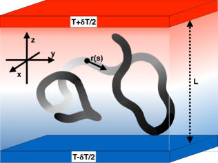
We develop a theory to assess the effects of GCF on a self-avoiding homopolymer with $N$ monomers of size $a_{0}$ confined between two parallel thermal conducting plates separated by a distance $L$ with a uniform temperature gradient, $\nabla T$ (Fig. 1). We assume that the fluid is a good solvent for the polymer, implying that the radius of gyration of the polymer is $R_{g}\sim a_{0}N^{\nu}$ with $\nu\approx 0.6$ if $\nabla T=0$; furthermore, we ignore the effect of confinement, which is to say that $\frac{L}{R_{g}}\gg 1$. In this setup the polymer behaves as a Flory random coil. We show that the presence of the GCF induces an intramolecular attraction, which we predict to be sufficiently strong to overcome the conformational entropy of the polymer, thus inducing a genuine NE coil to globule transition. Such a transition, which is akin to a phase transition  de Gennes (1979), occurs in equilibrium ($\nabla T=0$) only when the solvent quality is changed from good to poor. For a fixed $N$, we predict that there is a critical temperature gradient, $\nabla T_{c}$, above which the polymer undergoes a coil $\rightarrow$ globule transition. The critical temperature gradient at which the monomer-solvent energetics nearly compensates for the monomer-monomer interactions is defined as the NE $\Theta$-point.

Consider a polymer chain (Fig. 1) dissolved in a fluid confined between two horizontal thermal conducting plates, located at $z=0$ and $z=L$ with stationary temperature gradient $\nabla T$ (The local average temperature, $T(z)$, is a linear function of the coordinate $z$). We ignore the presence of convection in the fluid, which is achieved by setting the temperature of the upper plate at a larger value than the the temperature of the lower plate.

We start with the Edwards Hamiltonian for a polymer chain,

$$\mathcal{H}_{E}=\frac{3k_{B}T}{2a_{0}^{2}}\int\limits_{0}^{N}\left(\frac{\partial{\bf r}}{\partial s}\right)^{2}ds+k_{B}T\mathcal{V}({\bf r}(s)),$$ (1)

where, ${\bf r}(s)$ is the position of the monomer $s$ (Fig. 1), $a_{0}$ is the monomer size, and $N$ is the number of monomers. The first term in Eq. (1) accounts for chain connectivity, and the second term represents volume interactions given by $\mathcal{V}({\bf r}(s))=\frac{v}{(2\pi a_{0}^{2})^{3/2}}\sum\limits_{s,s^{\prime}=0}^{N}\text{exp}[{-\frac{({\bf r}(s)-{\bf r}(s^{\prime}))^{2}}{2a_{0}^{2}}}]$. We consider a long polymer whose size, $R_{g}$, is much less than $L$. In this limit, it is known that $R_{g}\approx a_{0}N^{\nu}$ with $\nu\approx 0.6$ provided $v>0$ i.e., the polymer is in a good solvent. If $L/R_{g}\ll 1$ then the polymer swells with $R_{g}\sim a_{0}N^{\nu}$ with $\nu=3/4$ Corderio et al. (1997); Daoud and De Gennes (1977), a situation not considered here. In the presence of $\nabla T$, the interaction between two monomers at ${\bf r}_{1}={\bf r}(s_{1})$ and ${\bf r}_{2}={\bf r}(s_{2})$, is altered due to fluctuation-induced non-equilibrium forces. The additional effective pair potential due to GCF is $V({\bf r}_{1},{\bf r}_{2})$, which could be attractive or repulsive depending on the thermodynamic properties of the fluid.

In the presence of $\nabla T$, the non-equilibrium fluctuations in fluids are large and long ranged Dorfman et al. (1994). The NE fluctuations arise due to the coupling between the heat and the viscous modes. The former is caused by temperature fluctuations whereas the latter is due to velocity fluctuations, which is accounted by the convective term in the fluctuating-hydrodynamics equations Croccolo et al. (2016). In a one component fluid, two sound modes are encountered, associated with pressure fluctuations, in addition to heat and viscous mode Ortiz de Zárate and Sengers (2006); Chandrasekhar (1981). In normal fluids, sound modes are fast propagating, while the heat mode is the slow diffusive mode. Therefore, to deal with slow diffusive temperature fluctuations, we may neglect pressure fluctuations.

For a quiescent fluid, in the presence of a uniform temperature gradient $\nabla T$, the non-equilibrium contribution to the intensity of the temperature fluctuations varies with the wave number $k$, diverging as $k^{-4}$ in the limit $k\rightarrow 0$, as predicted theoretically Kirkpatrick et al. (1982); Law and Sengers (1989); Law and Nieuwoudt (1989); Belitz et al. (2005) and confirmed experimentally Law et al. (1990); Segre et al. (1992, 1993); Li et al. (1994); Vailati and Giglio (1996, 1997); Takacs et al. (2011); Cerbino et al. (2015). As a consequence, the long-range NE fluctuations induce significant Casimir-like forces in fluids, in the presence of temperature gradient. Such a GCF should have a dramatic effect on the size of the polymer.

The $L$-dependent NE fluctuation contribution to pressure, $P_{NE}(L)$, is given by Kirkpatrick et al. (2013, 2014, 2016a),

$$P_{NE}(L)=k_{B}T~{}A~{}L(\frac{\nabla T}{T})^{2}=k_{B}T\frac{A}{L}(\frac{\delta T}{T})^{2},~{}\text{with},$$ (2)

$$A=\frac{C_{P}T(\gamma-1)}{96\pi D_{T}(\nu+D_{T})}\left[1-\frac{1}{\alpha C_{p}}\left(\frac{\partial C_{P}}{\partial T}\right)_{P}+\frac{1}{\alpha^{2}}\left(\frac{\partial\alpha}{\partial T}\right)_{P}\right]$$

where, $\delta T$ is the temperature difference between the two plates (Fig. 1), $C_{P}$ is the isobaric specific heat capacity, $D_{T}$ is the thermal diffusivity, $\gamma$ is the ratio of isobaric and isochoric heat capacities, and $\alpha$ is the thermal expansion coefficient. For a fixed value of the temperature gradient, the NE pressure grows with increasing $L$. This anomalous behavior is a reflection of the very long-range spatial correlations in a fluid, in the presence of a temperature gradient. For a fixed value of the temperature difference $\delta T$ between the plates, the giant NE Casimir pressure varies as $L^{-1}$, which is much longer ranged than the $f_{EM}\sim L^{-4}$ dependence for electromagnetic Casimir forces, or a $f_{c}\sim L^{-3}$ dependence for the critical Casimir forces Fisher and de Gennes (1978).

If a polymer is inserted between the plates then the average force between two monomers, which are at a distance $\mid z_{1}-z_{2}\mid$ apart, is given by  Kirkpatrick et al. (2016b),

$$\mathcal{F}_{12}=-4\pi a_{0}^{2}P_{NE}(L)\frac{|z_{1}-z_{2}|}{L},$$ (3)

where $a_{0}^{2}$ is the size of the monomer and $z_{1}$ and $z_{2}$ are the positions of the two monomers on polymer chain. We assume that $\nabla T$ acts over a distance $|z_{1}-z_{2}|$ such that $z_{1}=L/2-\delta/2$ and $z_{2}=L/2-\delta/2$ with $a_{0}\ll\delta\ll L$. The force can be attractive or repulsive depending on the nature of the fluid, which we discuss further below.

In order to calculate the $R_{g}$ of the polymer in the slit with $\nabla T$ we use an approximate method introduced by Edwards and Singh (ES) Edwards and Singh (1979). The ES method is a variational type calculation that represents the exact Hamiltonian by a Gaussian chain. The effective monomer size in the variational Hamiltonian is determined as follows. Consider a virtual chain without excluded volume interactions, with the radius of gyration $\langle R_{g}^{2}\rangle=Na^{2}/6$ Edwards and Singh (1979), described by the Hamiltonian

$$\mathcal{H}_{v}=\frac{3k_{B}T}{2a^{2}}\int\limits_{0}^{N}\left(\frac{\partial{\bf r}}{\partial s}\right)^{2}ds,$$ (4)

where $a$ is the effective monomer size. We split the deviation $\mathcal{W}$ between the virtual chain Hamiltonian and the exact Hamiltonian as,

$$\mathcal{H}-\mathcal{H}_{v}=k_{B}T\mathcal{W}=k_{B}T(\mathcal{W}_{1}+\mathcal{W}_{2}),$$ (5)

where

$$\mathcal{W}_{1}=\frac{3}{2}\left(\frac{1}{a_{0}^{2}}-\frac{1}{a^{2}}\right)\int\limits_{0}^{N}\left(\frac{\partial{\bf r}}{\partial s}\right)^{2}ds,$$ (6)

$$\mathcal{W}_{2}=\mathcal{V}({\bf r}(s))+\sum\limits_{s,s^{\prime}=0}^{N}V({\bf r}(s)-{\bf r}(s^{\prime})).$$

The term $V({\bf r}(s)-{\bf r}(s^{\prime}))$ in Eq. (6) is the contribution from the GCF, and is obtained by integrating $\mathcal{F}_{12}$ in Eq.  (3) with respect to the $z$-variable. The radius of gyration is $R_{g}^{2}=\frac{1}{N}\int\limits_{0}^{N}\langle{\bf r}^{2}(s)\rangle ds$, with the average being $\langle{\bf r}^{2}(s)\rangle=\frac{\int r^{2}e^{-\mathcal{H}_{v}/k_{B}T}e^{\mathcal{-W}}\delta{\bf r}}{\int e^{-\mathcal{H}_{v}/k_{B}T}e^{\mathcal{-W}}\delta{\bf r}}=\frac{\langle{\bf r}^{2}(s)e^{\mathcal{-W}}\rangle_{v}}{\langle e^{\mathcal{-W}}\rangle_{v}}$, where, $\langle\cdots\rangle_{v}$ denotes the average over $\mathcal{H}_{v}$.

Assuming that the deviation $\mathcal{W}$ is ’small’, we can calculate the average $R_{g}$ to first order in $\mathcal{W}$. The result is, $\langle{\bf r}^{2}(s)\rangle\approx\frac{\langle{\bf r}^{2}(s)(1-\mathcal{W})\rangle_{v}}{\langle(1-\mathcal{W})\rangle_{v}}\approx\langle{\bf r}^{2}(s)(1-\mathcal{W})\rangle_{v}\langle(1+\mathcal{W})\rangle_{v}$, leading to,

$$\langle R_{g}^{2}\rangle=\frac{1}{N}\int\limits_{0}^{N}\langle{\bf r}^{2}(s)\rangle ds$$ (7)

$$=\frac{1}{N}\int\limits_{0}^{N}[\langle{\bf r}^{2}(s)\rangle_{v}+\langle{\bf r}^{2}(s)\rangle_{v}\langle\mathcal{W}\rangle_{v}-\langle{\bf r}^{2}(s)\mathcal{W}\rangle_{v}]ds.$$

If we choose the effective monomer size $a$ in $\mathcal{H}_{v}$ such that the first order correction (second and third terms in the second line of Eq. (7)) vanishes, then the size of the chain is, $\langle R_{g}^{2}\rangle=Na^{2}/6$. This is an estimate of the exact $\langle R_{g}^{2}\rangle$, and is an approximation as we have neglected $\mathcal{W}^{2}$ and higher powers of $\mathcal{W}$. However, following the analysis in  Edwards and Singh (1979) we can assume that inclusion of higher order terms merely renormalizes the coefficients of the dependence of $R_{g}$ on $N$ and $\nabla T$ without altering the essential qualitative results. Thus, in the ES theory, we find $a$ by setting the first order correction (second and third terms in the second line of Eq. (7)) to zero. The resulting equation should be solved in a self-consistent manner for $a$, and is given by Edwards and Singh (1979):

$$\frac{1}{a_{0}^{2}}-\frac{1}{a^{2}}=\frac{\frac{1}{N}\int\limits_{0}^{N}[\langle{\bf r}^{2}(s)\rangle_{v}\langle\mathcal{W}_{2}\rangle_{v}-\langle{\bf r}^{2}(s)\mathcal{W}_{2}\rangle_{v}]ds}{\frac{a^{2}}{N}\int_{0}^{N}ds\ \langle{\bf r}^{2}(s)\rangle_{v}}.$$ (8)

Calculating the averages in the Fourier space (${\bf r}_{n}=\frac{1}{N}\int\limits_{1}^{N}\cos\left({\frac{\pi ns}{N}}\right){\bf r}(s)ds$; ${\bf r}(s)=2\sum\limits_{n=1}^{N}\cos\left({\frac{\pi ns}{N}}\right){\bf r}_{n}$; $R_{g}^{2}=2\sum\limits_{n}\langle|{{\bf r}_{n}}^{2}|\rangle$), we obtain

$$\frac{1}{a_{0}^{2}}-\frac{1}{a^{2}}=\sum\limits_{s,s^{\prime}=0}^{N}\left[v\frac{C^{ss^{\prime}}_{1}}{(C^{ss^{\prime}})^{5/2}}-A\left(\frac{\nabla T}{T}\right)^{2}C^{ss^{\prime}}_{2}\right]$$ (9)

where, $C^{ss^{\prime}}_{1}=\frac{\sqrt{2}N}{3a^{5}\pi^{5/2}\sum\limits_{n=1}^{N}\frac{1}{n^{2}}}\sum\limits_{n=1}^{N}2\frac{1-\cos[n\pi(s-s^{\prime})/N]}{n^{4}}$, $C^{ss^{\prime}}=\frac{2N}{3\pi^{2}}\sum\limits_{n=1}^{N}\frac{1-\cos[n\pi(s-s^{\prime})/N]}{n^{2}}+\frac{a_{0}^{2}}{a^{2}}$, $C^{ss^{\prime}}_{2}=\frac{4a_{0}^{2}N}{{9\pi\sum\limits_{n=1}^{N}\frac{1}{n^{2}}}}\sum\limits_{n=1}^{N}2\frac{1-\cos[n\pi(s-s^{\prime})/N]}{n^{4}}$, and $v=\frac{4}{3}\pi a_{0}^{3}$.

The best estimate for the effective monomer size $a$ can be obtained using Eq. (9). The $\Theta$-point signals the transition from a coil to a globule. We use the definition of the $\Theta$-point to assess the condition for collapse in terms of temperature gradient, instead of solving the complicated Eq. (9) numerically. The volume interactions are on the right hand side of Eq. (9). At the $\Theta$-point, the $v$-term should exactly balance the GCF term. Since at the $\Theta$-point the dimensions of the chain is ideal, implying $a=a_{0}$, we can substitute this value for $a$ in the $v$- and the GCF terms, and equate the two . The result yields an expression for the $\Theta$-point as a function of $\nabla T$. Thus, from Eq. (9) the temperature gradient at which two body repulsion ($v$-term) equals two body interaction (Casimir-term) is,

$$\Big{(}\frac{\nabla T_{c}}{T}\Big{)}^{2}=\frac{\sum\limits_{s,s^{\prime}=0}^{N}v\frac{C^{ss^{\prime}}_{1}}{(C^{ss^{\prime}})^{5/2}}}{A\sum\limits_{s,s^{\prime}=0}^{N}C^{ss^{\prime}}_{2}}.$$ (10)

The numerator in Eq. (10) is a consequence of chain connectivity, and the denominator encodes the fluctuation induced effect, determining the extent to which the sizes in extended states change with temperature gradient. Clearly, $\nabla T_{c}$ is determined by the fluid properties through $A$. The results in Eq. (9) can be used to obtain the dependence of $\nabla T_{c}$ on $N$. Scaling $n$ by $N$, it can be shown that $C^{ss^{\prime}}_{1}\sim N$. Similarly, $C^{ss^{\prime}}_{2}\sim N$ and $C^{ss^{\prime}}\sim N$. From these results it follows that

$$\nabla T_{c}\sim N^{-\frac{5}{4}}.$$ (11)

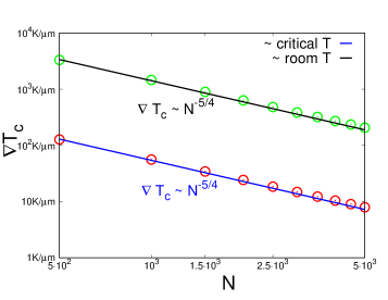
To estimate the critical temperature gradient $\nabla T_{c}$, implied by Eq. (10), we consider the example of fluid neopentane, for which accurate light scattering experiments of the non-equilibrium temperature fluctuations are available Lem (Eq2). Using available data for the thermodynamic and transport properties for neopentane [described in the Supplementary Information (SI) Lem (Eq2)], we calculated the numerical value of temperature gradient $\nabla T$ using Eq. (10) at the $\Theta$ transition. As an example consider the parameters given in Table S1 in the SI Lem (Eq2). The predicted value (Eq. 10) for $\nabla T_{c}$ near the critical temperature for neopentane ranges from $\approx(35-8)~{}K\cdot{\mu m}^{-1}$ for $N$ between 1500 to 5000 (see the red line in Fig. 2). This falls within the experimentally achievable range of temperature gradient Talbot et al. (2017).

Figure 2: The critical temperature gradient $\nabla T_{c}$ decreases with $N$ as $N^{-5/4}$. Red and green circles are the predicted values for $\nabla T_{c}$ for neopentane fluid at temperature 433K and 300K respectively for different polymer chains. The calculations are done for polystyrene for which $a_{0}$, the monomer size, is $\approx$ 17Å Suzuki et al. (2013).

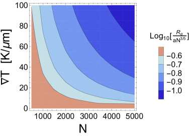
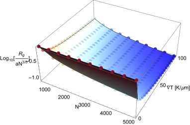
The GCF term is negative for the fluid neopentane, implying that a polymer for which neopentane is a good solvent (such as polyisoprene or polystyrene) is predicted to undergo a coil to globule transition when $\nabla T$ exceeds $\nabla T_{c}$. Fig. 3 shows that the size of the chain ($R_{g}$) decreases continuously with increasing $\nabla T$, implying non-equilibrium fluctuations driven collapse of a polymer chain in a fluid. The GCF term is very sensitive to the thermodynamic properties of the relevant fluid. For example, for toluene, the GCF is positive for temperature below 310K at 26 MPa pressure, implying fluctuation-induced interactions between monomers are repulsive (see the SI for the values for toluene). In this case, the chain is in a good solvent even if $\nabla T\neq 0$, and we predict that there ought to be no coil-globule transition for any value of $\nabla T$. Above 310K temperature, GCF term is negative, implying fluctuation induced interactions between monomers are attractive and the coil-globule transition would occur when $\nabla T$ exceeds $\nabla T_{c}$. These spectacularly contrasting predictions can be verified using currently available techniques using standard polymers (polystyrene or polyisoprene) in organic solvents.

(a)

(b)

Figure 3: The top panel shows that the radius of gyration ($R_{g}$) for ten different chain lengths (from N= 500 to N=5000). decreases continuously with increasing temperature gradient. The bottom panel is a three dimensional plot displaying $R_{g}$ as a function of $N$ and $\nabla T$. These figures show significant contraction of the chain over the span of experimentally realizable values of the temperature gradient.

In summary, we predict that the non-equilibrium giant Casimir force between monomers in a homopolymer could induce a coil to globule transition in a polymer that exists in a swollen random coil state in the absence of the temperature gradient. The interactions leading to the predicted dramatic transition is due to attractive long ranged interactions between the monomers due thermal fluctuations in the NE steady state. The fluctuation induced force could be attractive or repulsive depending on the thermodynamic properties of the relevant fluid. Our theory predicts that above a critical value of the temperature gradient monomer-monomer attractive interactions will overcome the chain conformational entropy, inducing a coil to globule transition in certain solvents. The easiest experiment to imagine is a polymer in a custom-made cell in a fluid with the system initially in thermal equilibrium. A vertical temperature difference $\Delta T$ across the cell is then imposed. Assuming the temperature gradient in the solvent is quickly established, we predict that the polymer will respond to it and collapse or not according to our theoretical considerations. We should emphasize that because our predictions suggest a large change in the size of the polymer the effects are far from being subtle. Consequently, we envision that our predictions are amenable to test by standard light scattering experiments. Finally we note that a polymer in liquid mixtures can also be profoundly affected by concentration fluctuations. In this case, a temperature gradient induces long-range concentration fluctuations through the Soret effect. We hope to report the consequences of the Soret effect on the size of a polymer elsewhere.

I Acknowledgements

This work was supported by the National Science Foundation under Grant Nos. DMR-1401449 and CHE-16-36424. DT acknowledges additional support from the Collie-Welch Regents Chair (F-0019).

II Sign of the Force and Value of the Critical Temperature Gradient in Neopentane and Toluene.

In order to establish whether the long-range interactions induced by the thermal gradient are attractive or repulsive, we need to evaluate the sign of the parameter $A$ [see Eq. (2) in the main text]. Because $C_{P},\nu,D_{T},(\gamma-1)>0$, the sign of $A$ depends on,

$$\bar{A}=\Big{[}1-\frac{1}{\alpha C_{P}}\Big{(}\frac{\partial C_{P}}{\partial T}\Big{)}_{P}+\frac{1}{\alpha^{2}}\Big{(}\frac{\partial\alpha}{\partial T}\Big{)}_{P}\Big{]}.$$ (S1)

The value of $\bar{A}$ depends on the thermodynamic state of the system (namely, temperature and density) and on the nature of the solvent. We consider the fluids neopentane and toluene. The Helmholtz free energy [$F=F(V,T)$] for both of these solvents are provided in Lemmon and Span (2006) as a function of volume and temperature. Because to evaluate $\bar{A}$ we need derivatives of $C_{P}$ and $\alpha$ as a function of $T$ along an isobaric path, we derived an equation to extract $\Big{(}\frac{\partial C_{P}}{\partial T}\Big{)}_{P}$ and $\Big{(}\frac{\partial\alpha}{\partial T}\Big{)}_{P}$ as a function of terms involving only derivatives with respect to $T$ and $V$ along isochoric and isothermal paths, respectively. Let $\phi=\phi(V,T)$ be any function of $V$ and $T$. We show below that,

$$\Big{(}\frac{\partial\phi}{\partial T}\Big{)}_{P}=\Big{(}\frac{\partial\phi}{\partial T}\Big{)}_{V}-\Big{(}\frac{\partial\phi}{\partial V}\Big{)}_{T}\frac{\Big{[}\frac{\partial}{\partial V}\Big{(}\frac{\partial F}{\partial T}\Big{)}_{V}\Big{]}_{T}}{\Big{(}\frac{\partial^{2}F}{\partial V^{2}}\Big{)}_{T}}.$$ (S2)

Plugging in Eq. S2 $C_{P}$ and $\alpha$ in place for $\phi$, and using the data in Lemmon and Span (2006) we obtain $\bar{A}$ (note that in Lemmon and Span (2006) there is an expression for the molar heat capacity at constant pressure, but not for $\alpha$; we can use Eq. S2 to extract $\alpha$ by substituting $\phi$ with $V$ and dividing the result by the volume; furthermore, to avoid confusion note that $\alpha$ is used in Lemmon and Span (2006) to indicate the Helmholtz free energy).

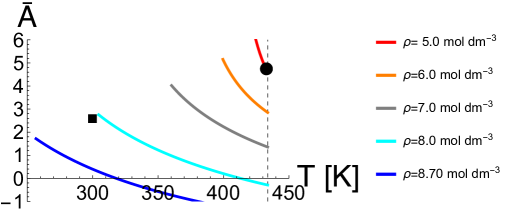
The value of $\bar{A}$ for neopentane is shown in Fig. S1 as a function of temperature at different concentrations. Clearly, we can find thermodynamic states for fluid neopentane with $\bar{A}>0$, which implies that the force is attractive and thus that for a supercritical thermal gradient the fluctuations in the NESS should induce the collapse of the polymer. Note also that at large concentrations of neopentane it is possible to manipulate the sign of $\bar{A}$ by changing the overall temperature of the system.

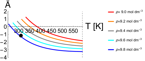
In contrast, for toluene we can readily find $\bar{A}<0$, although small changes in the temperature change the sign of $\bar{A}$. Hence, small changes in the average temperature at constant thermal gradient can change the sign of the fluctuation-induced force from attractive to repulsive (see blue line in Fig. S1, and Fig. S2), thus effectively changing the quality of the solvent from bad to good, which is triggered by non-equilibrium fluctuations.

To provide a numerical estimate of the critical gradient, we need to compute the coefficient $A$, which requires estimating also the kinematic viscosity and thermal diffusivity. We considered neopentane at room temperature ($T=300\mathrm{K}$) and $\rho=8.0927~{}\mathrm{mol}\cdot\mathrm{dm^{-3}}$ (see black square in Fig. S1), and at a lower density ($\rho=4.2647~{}\mathrm{mol}\cdot\mathrm{dm^{-3}}$) close to the critical temperature ($T=433\mathrm{K}$) (see black circle in Fig. S1). The thermodynamic and transport coefficients were obtained from the online server of the National Institute of Standards and Technology (NIST) NIS . The resulting parameters (see Table 1) yield $A\approx 85~{}\mathrm{nm^{-2}}$ in near-critical conditions, and $A\approx 6.0\cdot 10^{-2}~{}\mathrm{nm^{-2}}$ at room temperature. The larger value of $A$ close to the critical point accounts for the smaller critical gradient estimated in the main text (see Fig. 2). Similarly, we report thermodynamics and transport coefficients for liquid toluene at $T=310\mathrm{K}$ and $\rho=9.75~{}\mathrm{mol}\cdot\mathrm{dm^{-3}}$ (see Table 1), which results in a negative value of $A$ ($A\approx-5.8\cdot 10^{-3}~{}\mathrm{nm^{-2}}$) indicating that in this thermodynamic state the presence of the thermal gradient does not modify the quality of the solvent.

III Derivation of Eq. S2.

In order to derive Eq. S2, we consider the following three identities, which hold for any function $\phi=\phi(x,y)$,

$$\Big{(}\frac{\partial\phi}{\partial u}\Big{)}_{y}=\Big{(}\frac{\partial\phi}{\partial x}\Big{)}_{y}\Big{(}\frac{\partial x}{\partial u}\Big{)}_{y};$$ (S3)

$$\Big{(}\frac{\partial\phi}{\partial x}\Big{)}_{v}=\Big{(}\frac{\partial\phi}{\partial x}\Big{)}_{y}+\Big{(}\frac{\partial\phi}{\partial y}\Big{)}_{x}\Big{(}\frac{\partial y}{\partial x}\Big{)}_{v};\\$$ (S4)

$$\Big{(}\frac{\partial\phi}{\partial x}\Big{)}_{y}=\frac{1}{\Big{(}\frac{\partial x}{\partial\phi}\Big{)}_{y}}.$$ (S5)

Let $x=T$, $y=V$, and $v=P$, then from Eq. S4,

$$\Big{(}\frac{\partial\phi}{\partial T}\Big{)}_{P}=\Big{(}\frac{\partial\phi}{\partial T}\Big{)}_{V}+\Big{(}\frac{\partial\phi}{\partial V}\Big{)}_{T}\Big{(}\frac{\partial V}{\partial T}\Big{)}_{P}.$$ (S6)

With the aid of the Maxwell relation $\Big{(}\frac{\partial V}{\partial T}\Big{)}_{P}=-\Big{(}\frac{\partial S}{\partial P}\Big{)}_{T}$ (see Callen (1960)) we get,

$$\Big{(}\frac{\partial\phi}{\partial T}\Big{)}_{P}=\Big{(}\frac{\partial\phi}{\partial T}\Big{)}_{V}-\Big{(}\frac{\partial\phi}{\partial V}\Big{)}_{T}\Big{(}\frac{\partial S}{\partial P}\Big{)}_{T},$$ (S7)

where $S$ is the entropy.

Let $\phi=S$, $x=V$, $u=P$, and $y=T$, then from Eq. S3,

$$\Big{(}\frac{\partial S}{\partial P}\Big{)}_{T}=\Big{(}\frac{\partial S}{\partial V}\Big{)}_{T}\Big{(}\frac{\partial V}{\partial P}\Big{)}_{T},$$ (S8)

and using Eq. S5 for the second term on the r.h.s. we obtain,

$$\Big{(}\frac{\partial S}{\partial P}\Big{)}_{T}=\frac{\Big{(}\frac{\partial S}{\partial V}\Big{)}_{T}}{\Big{(}\frac{\partial P}{\partial V}\Big{)}_{T}}.$$ (S9)

Let $F=F(V,T)$ be the Helmholtz free energy, then by plugging Eq. S9 in Eq. S7 and substituting $P=-\Big{(}\frac{\partial F}{\partial V}\Big{)}_{T}$ and $S=-\Big{(}\frac{\partial F}{\partial T}\Big{)}_{V}$ we obtain Eq. S2.

III.1

III.1.1

Figure S1: (a) The value of $\bar{A}$ as a function of density and temperature for fluid neopentane. Different lines correspond to different densities. Each curve is shown in the temperature range corresponding to the fluid phase web . The dot and the square correspond to the values at which the evaluation of $A$ was performed; the dot has been obtained using ($T=433\mathrm{K}$, $\rho=4.2647~{}\mathrm{mol}\cdot\mathrm{dm^{-3}}$), and the value of $A$ for the thermodynamic state ($T=300\mathrm{K}$, $\rho=8.0927~{}\mathrm{mol}\cdot\mathrm{dm^{-3}}$) is shown as a square. The dashed vertical line shows the critical temperature, $T_{c}=433.74\mathrm{K}$ web .

Figure S2: Same as Fig. S1, but for toluene. The critical temperature is $T_{c}=591.75~{}\mathrm{K}$ web ). The dot shows the thermodynamic state ($T=310\mathrm{K}$, $\rho=9.75~{}\mathrm{mol}\cdot\mathrm{dm^{-3}}$).

Table 1: Parameters for liquid neopentane and toluene. The first column indicates the thermodynamic or transport coefficient. $\eta$ is the viscosity; the kinematic viscosity is $\nu=\eta/\rho_{m}$, with $\rho_{m}$ mass density. $k$ is the thermal conductivity, which is related to the thermal diffusivity by $D_{T}=k/(\rho C_{P})$. $c_{P}$ and $c_{V}$ are the molar heat capacities at constant pressure and volume, respectively, and $C_{P}$ is the specific heat capacity. The second column reports the values of the coefficients at $T=300\mathrm{K}$ and $\rho=8.0927~{}\mathrm{mol}\cdot\mathrm{dm^{-3}}$ for neopentane. The coefficients for neopentane in near-critical conditions are reported in the third column ($T=433\mathrm{K}$, $\rho=4.2647~{}\mathrm{mol}\cdot\mathrm{dm^{-3}}$). The last column shows the parameters for toluene at $T=310\mathrm{K}$ and $\rho=9.75~{}\mathrm{mol}\cdot\mathrm{dm^{-3}}$. The symbol “^†” indicates a quantity obtained from the NIST website NIS . If a coefficient was computed using the Helmholtz free energy from Lemmon and Span (2006), the symbol “^‡” is used. If a coefficient has been obtained in two different ways, the result from NIST are displayed; the value yielded by the Helmholtz free energy from Lemmon and Span (2006) is within the error bar reported. The results from NIST have been obtained at fixed temperature and pressure, while those using the Helmholtz free energy imposing the density and temperature. For both thermodynamic states (second and third column), the density computed with the NIST website was within error bar from the density used for the Helmholtz free energy.

	Neopentane	Neopentane	Toluene
parameter	$T=300\mathrm{K}$ $\rho=8.0927~{}\mathrm{mol}\cdot\mathrm{dm^{-3}}$	$T=433\mathrm{K}$ $\rho=4.2647~{}\mathrm{mol}\cdot\mathrm{dm^{-3}}$	$T=310\mathrm{K}$ $\rho=9.75~{}\mathrm{mol}\cdot\mathrm{dm^{-3}}$
$\eta^{\dagger}~{}~{}[\mathrm{Pa}\cdot\mathrm{s}]$	$(2.4141\pm 0.0061)\cdot 10^{-4}$	$(3.75\pm 0.23)\cdot 10^{-5}$	$(7.90\pm 0.13)\cdot 10^{-4}$
$k^{\dagger}~{}~{}[\mathrm{W}\cdot\mathrm{m^{-1}}\cdot\mathrm{K^{-1}}]$	$(9.333\pm 0.015)\cdot 10^{-2}$	$(6.68\pm 0.30)\cdot 10^{-2}$	$0.14856\pm 0.00067$
$c_{P}^{\dagger,\ddagger}~{}[\mathrm{J}\cdot\mathrm{mol^{-1}}\cdot\mathrm{K^{-1}}]$	$167.0\pm 2.0$	$770\pm 320$	$156.7\pm 4.1$
$c_{V}^{\ddagger}~{}~{}[\mathrm{J}\cdot\mathrm{mol^{-1}}\cdot\mathrm{K^{-1}}]$	$124.7$	$176$	$122.2$
$\alpha^{\dagger,\ddagger}~{}[\mathrm{K^{-1}}]$	$(1.898\pm 0.051)\cdot 10^{-3}$	$(7.6\pm 4.4)\cdot 10^{-2}$	$(7.97\pm 0.17)\cdot 10^{-4}$

References

- Casimir (1948) H. B. G. Casimir, Proc. K. Ned. Akad. Wet. 51, 793 (1948).
- Kardar and Golestanian (1999) M. Kardar and R. Golestanian, Rev. Mod. Phys. 71, 1233 (1999).
- Lifshitz (1956) E. M. Lifshitz, Sov. Phys. JETP 2, 73 (1956).
- Dzyaloshinskii et al. (1961) I. Dzyaloshinskii, E. Lifshitz, and L. Pitaevskii, Adv. Phys. 10, 165 (1961).
- Fisher and de Gennes (1978) M. Fisher and P. G. de Gennes, C. R. Seances Acad. Sci. B 287, 207 (1978).
- Krech (1994) M. Krech, The Casimir Effect in Critical Systems (World Scientific, Singapore, 1994).
- Kirkpatrick et al. (2013) T. R. Kirkpatrick, J. M. Ortiz de Zárate, and J. V. Sengers, Phys. Rev. Lett. 110, 235902 (2013).
- Kirkpatrick et al. (2014) T. R. Kirkpatrick, J. M. Ortiz de Zárate, and J. V. Sengers, Phys. Rev. E 89, 022145 (2014).
- Kirkpatrick et al. (2016a) T. R. Kirkpatrick, J. M. Ortiz de Zárate, and J. V. Sengers, Phys. Rev. E 93, 012148 (2016a).
- Giddings (1993) J. C. Giddings, Science 260, 1456 (1993).
- Baaske et al. (2007) P. Baaske, F. Weinert, S. Duhr, M. R. K. Lemke, and D. Braun, Proc. Natl. Acad. Sci. 104, 9346 (2007).
- Budin et al. (2009) I. Budin, R. Bruckner, and J. Szostak, J. Am. Chem. Soc. 131, 9628 (2009).
- Jiang et al. (2009) H.-R. Jiang, H. Wada, N. Yoshinaga, and M. Sano, Phys. Rev. Lett. 102, 208301 (2009).
- Kumaki et al. (1996) J. Kumaki, T. Hashimoto, and S. Granick, Phys. Rev. Lett. 77, 1990 (1996).
- Toda et al. (2012) A. Toda, K. Taguchi, and H. Kajioka, Macromolecules 45, 852 (2012).
- Piazza and Parola (2008) R. Piazza and A. Parola, J. Phys.: Condens. Matter 20, 153102 (2008).
- de Gennes (1979) P. G. de Gennes, Scaling Concepts in Polymer Physics (Cornell University Press, 1979).
- Corderio et al. (1997) C. Corderio, M. Molisana, and D. Thirumalai, J. Phys. II France 7, 433 (1997).
- Daoud and De Gennes (1977) M. Daoud and P.-G. De Gennes, J. Phys. (Paris) 38(1), 85 (1977).
- Dorfman et al. (1994) J. R. Dorfman, T. R. Kirkpatrick, and J. V. Sengers, Annu. Rev. Phys. Chem. 45, 213 (1994).
- Croccolo et al. (2016) F. Croccolo, J. M. Ortiz de Zárate, and J. Sengers, Eur. Phys. J. E 39, 125 (2016).
- Ortiz de Zárate and Sengers (2006) J. M. Ortiz de Zárate and J. V. Sengers, Hydrodynamic Fluctuations in Fluids and Fluid Mixtures (Elsevier, Amsterdam, 2006).
- Chandrasekhar (1981) S. Chandrasekhar, Hydrodynamic and Hydromagnetic Stability (Oxford University Press/Dover, Oxford, 1981).
- Kirkpatrick et al. (1982) T. R. Kirkpatrick, E. G. D. Cohen, and J. R. Dorfman, Phys. Rev. A 26, 995 (1982).
- Law and Sengers (1989) B. M. Law and J. V. Sengers, J. Stat. Phys. 57, 531 (1989).
- Law and Nieuwoudt (1989) B. M. Law and J. C. Nieuwoudt, Phys. Rev. A 40, 3880 (1989).
- Belitz et al. (2005) D. Belitz, T. R. Kirkpatrick, and T. Votja, Rev. Mod. Phys. 77, 579 (2005).
- Law et al. (1990) B. M. Law, P. N. Segre, R. W. Gammon, and J. V. Sengers, Phys. Rev. A 41, 816 (1990).
- Segre et al. (1992) P. N. Segre, R. W. Gammon, J. V. Sengers, and B. M. Law, Phys. Rev. A 45, 714 (1992).
- Segre et al. (1993) P. N. Segre, R. W. Gammon, and J. V. Sengers, Phys. Rev. E 47, 1026 (1993).
- Li et al. (1994) W. B. Li, P. N. Segre, R. W. Gammon, and J. V. Sengers, Physica A 204, 399 (1994).
- Vailati and Giglio (1996) A. Vailati and M. Giglio, Phys. Rev. Lett. 77, 1484 (1996).
- Vailati and Giglio (1997) A. Vailati and M. Giglio, Nature (London) 390, 262 (1997).
- Takacs et al. (2011) C. J. Takacs, A. Vailati, R. Cerbino, S. Mazzoni, M. Giglio, and D. S. Cannell, Phys. Rev. Lett. 106, 244502 (2011).
- Cerbino et al. (2015) R. Cerbino, Y. Sun, A. Donev, and A. Vailati, Sci. Rep. 5, 14486 (2015).
- Kirkpatrick et al. (2016b) T. R. Kirkpatrick, J. M. Ortiz de Zárate, and J. V. Sengers, Phys. Rev. E 93, 032117 (2016b).
- Edwards and Singh (1979) S. F. Edwards and P. Singh, J. Chem. Soc., Faraday Trans. 2 75, 1001 (1979).
- Lem ( Eq2) (See Supplemental Material at http://link.aps.org/ for available data for thermodynamic and transport properties for neopentane and toluene, as well as the details of the calculation of the parameter in Eq.(2).).
- Talbot et al. (2017) E. L. Talbot, J. Kotar, L. Parolini, L. Di Michele, and P. Cicuta, Nature Communications 8, 15351 (2017).
- Suzuki et al. (2013) J. Suzuki, A. Takano, and Y. Matsushita, J. Chem. Phys. 139, 184904 (2013).
Supplemental Materials:
- Lemmon and Span (2006) E. W. Lemmon and R. Span, Journal of Chemical & Engineering Data 51, 785 (2006).
- (2) “National institute of standards and technology,” http://wtt-pro.nist.gov/.
- Callen (1960) H. Callen, Thermodynamics (John Wiley & Sons, INC, 1960).
- (4) “National institute of standards and technology,” http://webbook.nist.gov/.