Robust Hypothesis Test for Nonlinear Effect
with Gaussian Processes
Abstract
This work constructs a hypothesis test for detecting whether an data-generating function belongs to a specific reproducing kernel Hilbert space , where the structure of is only partially known. Utilizing the theory of reproducing kernels, we reduce this hypothesis to a simple one-sided score test for a scalar parameter, develop a testing procedure that is robust against the mis-specification of kernel functions, and also propose an ensemble-based estimator for the null model to guarantee test performance in small samples. To demonstrate the utility of the proposed method, we apply our test to the problem of detecting nonlinear interaction between groups of continuous features. We evaluate the finite-sample performance of our test under different data-generating functions and estimation strategies for the null model. Our results reveal interesting connections between notions in machine learning (model underfit/overfit) and those in statistical inference (i.e. Type I error/power of hypothesis test), and also highlight unexpected consequences of common model estimating strategies (e.g. estimating kernel hyperparameters using maximum likelihood estimation) on model inference.
1 Introduction
We study the problem of constructing a hypothesis test for an unknown data-generating function , when is estimated with a black-box algorithm (specifically, Gaussian Process regression) from observations . Specifically, we are interested in testing for the hypothesis:
where are the function spaces for under the null and the alternative hypothesis. We assume only partial knowledge about . For example, we may assume is the space of functions depend only on , while claiming no knowledge about other properties (linearity, smoothness, etc) about . We pay special attention to the setting where the sample size is small.
This type of tests carries concrete significance in scientific studies. In areas such as genetics, drug trials and environmental health, a hypothesis test for feature effect plays a critical role in answering scientific questions of interest. For example, assuming for simplicity , an investigator might inquire the effect of drug dosage on patient’s biometric measurement (corresponds to the null hypothesis ), or whether the adverse health effect of air pollutants is modified by patients’ nutrient intake (corresponds to the null hypothesis ). In these studies, usually represents some complex, nonlinear biological process whose exact mathematical properties are not known. Sample size in these studies are often small , due to the high monetary and time cost in subject recruitment and the lab analysis of biological samples.
There exist two challenges in designing such a test. The first challenge arises from the low interpretability of the blackbox model. It is difficult to formulate a hypothesis about feature effect in these models, since the blackbox models represents implicitly using a collection of basis functions constructed from the entire feature vector , rather than a set of model parameters that can be interpreted in the context of some effect of interest. For example, consider testing for the interaction effect between and . With linear model , we can simply represent the interaction effect using a single parameter , and test for . On the other hand, Gaussian process (GP) (rasmussen_gaussian_2006, ) models using basis functions defined by the kernel function . Since is an implicit function that takes the entire feature vector as input, it is not clear how to represent the interaction effect in GP models. We address this challenge assuming belongs to a reproducing kernel Hilbert space (RKHS) governed by the kernel function , such that when , and otherwise. In this way, encode exactly the feature effect of interest, and the null hypothesis can be equivalently stated as . To test for the hypothesis, we re-formulate the GP estimates as the variance components of a linear mixed model (LMM) (liu_semiparametric_2007, ), and derive a variance component score test which requires only model estimates under the null hypothesis.
Clearly, performance of the hypothesis test depends on the quality of the model estimate under the null hypothesis, which give rise to the second challenge: estimating the null model when only having partial knowledge about . In the case of Gaussian process, this translates to only having partial knowledge about the kernel function . The performance of Gaussian process is sensitive to the choices of the kernel function . In principle, the RKHS generated by a proper kernel function should be rich enough so it contains the data-generating function , yet restrictive enough such that does not overfit in small samples. Choosing a kernel function that is too restrictive or too flexible will lead to either model underfit or overfit, rendering the subsequent hypothesis tests not valid. We address this challenge by proposing an ensemble-based estimator for we term Cross-validated Kernel Ensemble (CVEK). Using a library of base kernels, CVEK learns a proper from data by directly minimizing the ensemble model’s cross-validation error, therefore guaranteeing robust test performance for a wide range of data-generating functions.
The rest of the paper is structured as follows. After a brief review of Gaussian process and its connection with linear mixed model in Section 2, we introduce the test procedure for general hypothesis in Section 3, and its companion estimation procedure CVEK in Section 4. To demonstrate the utility of the proposed test, in section 5, we adapt our test to the problem of detecting nonlinear interaction between groups of continuous features, and in section 6 we conduct simulation studies to evaluate the finite-sample performance of the interaction test, under different kernel estimation strategies, and under a range of data-generating functions with different mathematical properties. Our simulation study reveals interesting connection between notions in machine learning and those in statistical inference, by elucidating the consequence of model estimation (underfit overfit) on the Type I error and power of the subsequent hypothesis test. It also cautions against the use of some common estimation strategies (most notably, selecting kernel hyperparameters using maximum likelihood estimation) when conducting hypothesis test in small samples, by highlighting inflated Type I errors from hypothesis tests based on the resulting estimates. We note that the methods and conclusions from this work is extendable beyond the Gaussian Process models, due to GP’s connection to other blackbox models such as random forest (davies_random_2014, ) and deep neural network wilson_deep_2015 .
2 Background on Gaussian Process
Assume we observe data from independent subjects. For the subject, let be a continuous response, be the set of continuous features that has nonlinear effect on . We assume that the outcome depends on features through below data-generating model:
| (1) |
and follows the Gaussian process prior governed by the positive definite kernel function , such that the function evaluated at the observed record follows the multivariate normal (MVN) distribution:
with covariance matrix . Under above construction, the predictive distribution of evaluated at the samples is also multivariate normal:
To understand the impact of and on , recall that Gaussian process can be understood as the Bayesian version of the kernel machine regression, where equivalently arise from the below optimization problem:
where is the RKHS generated by kernel function . From this perspective, is the element in a spherical ball in that best approximates the observed data . The norm of , , is constrained by the tuning parameter , and the mathematical properties (e.g. smoothness, spectral density, etc) of are governed by the kernel function . It should be noticed that although may arise from , the probability of the Gaussian Process is 0 (lukic_stochastic_2001).
Gaussian Process as Linear Mixed Model
liu_semiparametric_2007 argued that if define , can arise exactly from a linear mixed model (LMM):
| (2) |
Therefore can be treated as part of the LMM’s variance components parameters. If is correctly specified, then the variance components parameters can be estimated unbiasedly by maximizing the Restricted Maximum Likelihood (REML)(lin_variance_1997, ):
| (3) |
where , and a vector whose all elements are 1. However, it is worth noting that REML is a model-based procedure. Therefore improper estimates for may arise when the family of kernel functions are mis-specified.
3 A recipe for general hypothesis
The GP-LMM connection introduced in Section 2 opens up the arsenal of statistical tools from Linear Mixed Model for inference tasks in Gaussian Process. Here, we use the classical variance component test (lin_variance_1997, ) to construct a testing procedure for the hypothesis about Gaussian process function:
| (4) |
We first translate above hypothesis into a hypothesis in terms of model parameters. The key of our approach is to assume that lies in a RKHS generated by a garrote kernel function (maity_powerful_2011, ), which is constructed by including an extra garrote parameter to a given kernel function. When , the garrote kernel function generates exactly , the space of functions under the null hypothesis. In order to adapt this general hypothesisio to their hypothesis of interest, practitioners need only to specify the form of the garrote kernel so that corresponds to the null hypothesis. For example, If , corresponds to the null hypothesis , i.e. the function does not depend on . (As we’ll see in section 5, identifying such is not always straightforward). As a result, the general hypothesis (4) is equivalent to
| (5) |
We now construct a test statistic for (5) by noticing that the garrote parameter can be treated as a variance component parameter in the linear mixed model. This is because the Gaussian process under garrote kernel can be formulated into below LMM:
where is the kernel matrix generated by . Consequently, we can derive a variance component test for by calculating the square derivative of with respect under (lin_variance_1997, ):
| (6) |
where . In this expression, , and is the null derivative kernel matrix whose entry is .
As discussed previously, misspecifying the null kernel function negatively impacts the performance of the resulting hypothesis test. To better understand the mechanism at play, we express the test statistic from (6) in terms of the model residual :
| (7) |
where we have used the fact harville_maximum_1977 . As shown, the test statistic is a scaled quadratic-form statistic that is a function of the model residual. If is too restrictive, model estimates will underfit the data even under the null hypothesis, introducing extraneous correlation among the ’s, therefore leading to overestimated and eventually underestimated p-value under the null. In this case, the test procedure will frequently reject the null hypothesis (i.e. suggest the existence of nonlinear interaction) even when there is in fact no interaction, yielding an invalid test due to inflated Type I error. On the other hand, if is too flexible, model estimates will likely overfit the data in small samples, producing underestimated residuals, an underestimated test statistic, and overestimated p-values. In this case, the test procedure will too frequently fail to reject the null hypothesis (i.e. suggesting there is no interaction) when there is in fact interaction, yielding an insensitive test with diminished power.
The null distribution of can be approximated using a scaled chi-square distribution using Satterthwaite method (zhang_hypothesis_2003, ) by matching the first two moments of :
with solution (see Appendix for derivation):
where and are the submatrices of the REML information matrix. Numerically more accurate, but computationally less efficient approximation methods are also available (bodenham_comparison_2016).
Finally, the p-value of this test is calculated by examining the tail probability of :
A complete summary of the proposed testing procedure is available in Algorithm 1.
Input: Null Kernel Matrix , Derivative Kernel Matrix , Data
Output: Hypothesis Test p-value
Step 1: Estimate Null Model using REML
Step 3: Compute p-value and reach conclusion
In light of the discussion about model misspecification in Introduction section, we highlight the fact that our proposed test (6) is robust against model misspecification under the alternative (lin_variance_1997, ), since the calculation of test statistics do not require detailed parametric assumption about . However, the test is NOT robust against model misspecification under the null, since the expression of both test statistic and the null distribution parameters still involve the kernel matrices generated by (see Algorithm 1). In the next section, we address this problem by proposing a robust estimation procedure for the kernel matrices under the null.
4 Estimating Null Kernel Matrix using Cross-validated Kernel Ensemble
Observation in (7) motivates the need for a kernel estimation strategy that is flexible so that it does not underfit under the null, yet stable so that it does not overfit under the alternative. To this end, we propose estimating using the ensemble of a library of fixed base kernels :
| (8) |
where is the kernel predictor generated by base kernel . In order to maximize model stability, the ensemble weights are estimated to minimize the overall cross-validation error of . We term this method the Cross-Validated Kernel Ensemble (CVEK). Our proposed method belongs to the well-studied family of algorithms known as ensembles of kernel predictors (EKP) evgeniou_bounds_2000 ; evgeniou_leave_2004 ; cortes_two-stage_2010 ; cortes_ensembles_2012 , but with specialized focus in maximizing the algorithm’s cross-validation stability. Furthermore, in addition to producing ensemble estimates , CVEK will also produce the ensemble estimate of the kernel matrix that is required by Algorithm 1. The exact algorithm proceeds in three stages as follows:
Stage 1: For each basis kernel in the library , we first estimate , the prediction based on kernel, where the tunning parameter is selected by minimizing the leave-one-out cross validation (LOOCV) error (elisseeff_leave-one-out_2002, ):
| (9) |
We denote estimate the final LOOCV error for kernel .
Stage 2: Using the estimated LOOCV errors , estimate the ensemble weights such that it minimizes the overall LOOCV error:
and produce the final ensemble prediction:
where is the ensemble hat matrix.
Stage 3: Using the ensemble hat matrix , estimate the ensemble kernel matrix by solving:
Specifically, if we denote and the eigenvector and eigenvalues of , then adopts the form (see Appendix for derivation):
5 Application: Testing for Nonlinear Interaction
Recall in Section 3, we assume that we are given a that generates exactly . However, depending on the exact hypothesis of interest, identifying such is not always straightforward. In this section, we revisit the example about interaction testing discussed in challenge 1 at the Introduction section, and consider how to build a for below hypothesis of interest
where is the "pure interaction" function that is orthogonal to main effect functions and . Recall as discussed previously, this hypothesis is difficult to formulate with Gaussian process models, since the kernel functions in general do not explicitly separate the main and the interaction effect. Therefore rather than directly define , we need to first construct and that corresponds to the null and alternative hypothesis, and then identify the garrote kernel function such it generates exactly when and when .
We build using the tensor-product construction of RKHS on the product domain (gu_smoothing_2013, ), due to this approach’s unique ability in explicitly characterizing the space of "pure interaction" functions. Let be the RKHS of constant functions, and be the RKHS of centered functions for , respectively. We can then define the full space as . describes the space of functions that depends jointly on , and adopts below orthogonal decomposition:
where we have denoted and , respectively. We see that is indeed the space of“pure interaction" functions , since contains functions on the product domain , but is orthogonal to the space of additive main effect functions . To summarize, we have identified two function spaces and that has the desired interpretation:
We are now ready to identify the garrote kernel . To this end, we notice that both and are composite spaces built from basis RKHSs using direct sum and tensor product. If denote the reproducing kernel associated with , we can construct kernel functions for composite spaces and as (aronszajn_theory_1950, ):
and consequently, the garrote kernel function for :
| (10) |
Finally, using the chosen form of the garrote kernel function, the element of the null derivative kernel matrix is , i.e. the null derivative kernel matrix is simply the kernel matrix that corresponds to the interaction space. Therefore the score test statistic in (6) simplifies to:
| (11) |
where .
6 Simulation Experiment
We evaluated the finite-sample performance of the proposed interaction test in a simulation study that is analogous to a real nutrition-environment interaction study. We generate two groups of input features independently from standard Gaussian distribution, representing normalized data representing subject’s level of exposure to environmental pollutants and the levels of a subject’s intake of nutrients during the study. Throughout the simulation scenarios, we keep , and . We generate the outcome as:
| (12) |
where are sampled from RKHSs and , generated using a ground-truth kernel . We standardize all sampled functions to have unit norm, so that represents the strength of interaction relative to the main effect.
For each simulation scenario, we first generated data using and as above, then selected a to estimate the null model and obtain p-value using Algorithm 1. We repeated each scenario 1000 times, and evaluate the test performance using the empirical probability . Under null hypothesis , estimates the test’s Type I error, and should be smaller or equal to the significance level 0.05. Under alternative hypothesis , estimates the test’s power, and should ideally approach 1 quickly as the strength of interaction increases.
In this study, we varied to produce data-generating functions with different smoothness and complexity properties, and varied to reflect different common modeling strategies for the null model in addition to using CVEK. We then evaluated how these two aspects impact the hypothesis test’s Type I error and power.
Data-generating Functions
We sampled the data-generate function by using from Matérn kernel family (rasmussen_gaussian_2006, ):
with two non-negative hyperparameters . For a function sampled using Matérn kernel, determines the function’s smoothness, since is -times mean square differentiable if and only if . In the case of , Matérn kernel reduces to the Gaussian RBF kernel which is infinitely differentiable. determines the function’s complexity, this is because in Bochner’s spectral decomposition(rasmussen_gaussian_2006, )
| (13) |
determines how much weight the spectral density puts on the slow-varying, low-frequency basis functions. In this work, we vary to generate once-, twice, and infinitely-differentiable functions, and vary to generate functions with varying degree of complexity.
Modeling Strategies
Polynomial Kernels is a family of simple parametric kernels that is equivalent to the polynomial ridge regression model favored by statisticians due to its model interpretability. In this work, we use the linear kernel and quadratic kernel which are common choices from this family.
Gaussian RBF Kernels is a general-purpose kernel family that generates nonlinear, but infinitely differentiable (therefore very smooth) functions. Under this kernel, we consider two hyperparameter selection strategies common in machine learning applications: RBF-Median where we set to the sample median of , and RBF-MLE who estimates by maximizing the model likelihood.
Matérn and Neural Network Kernels are two flexible kernels favored by machine learning practitioners for their expressiveness. Matérn kernels generates functions that are more flexible compared to that of Gaussian RBF due to the relaxed smoothness constraint (snoek_practical_2012, ). In order to investigate the consequences of added flexibility relative to the true model, we use Matern 1/2, Matern 3/2 and Matern 5/2, corresponding to Matérn kernels with 1/2, 3/2, and 5/2. Neural network kernels (rasmussen_gaussian_2006, ) , on the other hand, represent a 1-layer Bayesian neural network with infinite hidden unit and probit link function, with being the prior variance on hidden weights. Therefore is flexible in the sense that it is an universal approximator for arbitrary continuous functions on the compact domain (hornik_approximation_1991, ). In this work, we denote NN 0.1, NN 1 and NN 10 to represent Bayesian networks with different prior constraints .
Result
The simulation results are presented graphically in Figure 1 and documented in detail in the Appendix. We first observe that for reasonably specified , the proposed hypothesis test always has the correct Type I error and reasonable power. We also observe that the complexity of the data-generating function (12) plays a role in test performance, in the sense that the power of the hypothesis tests increases as the Matérn ’s complexity parameter becomes larger, which corresponds to functions that put more weight on the complex, fast-varying eigenfunctions in (13).
We observed clear differences in test performance from different estimation strategies. In general, polynomial models (linear and quadratic) are too restrictive and appear to underfit the data under both the null and the alternative, producing inflated Type I error and diminished power. On the other hand, lower-order Matérn kernels (Matérn 1/2 and Matérn 3/2, dark blue lines) appear to be too flexible. Whenever data are generated from smoother , Matérn 1/2 and 3/2 overfit the data and produce deflated Type I error and severely diminished power, even if the hyperparameter are fixed at true value. Therefore unless there’s strong evidence that exhibits behavior consistent with that described by these kernels, we recommend avoid the use of either polynomial or lower-order Matérn kernels for hypothesis testing. Comparatively, Gaussian RBF works well for a wider range of ’s, but only if the hyperparameter is selected carefully. Specifically, RBF-Median (black dashed line) works generally well, despite being slightly conservative (i.e. lower power) when the data-generation function is smooth and of low complexity. RBF-MLE (black solid line), on the other hand, tends to underfit the data under the null and exhibits inflated Type I error, possibly because of the fact that is not strongly identified when the sample size is too small (wahba_spline_1990, ). The situation becomes more severe as becomes rougher and more complex, in the moderately extreme case of non-differentiable with , the Type I error is inflated to as high as 0.238. Neural Network kernels also perform well for a wide range of , and its Type I error is more robust to the specification of hyperparameters.
Finally, the two ensemble estimators CVEK-RBF (based on ’s with ) and CVEK-NN (based on ’s with ) perform as well or better than the non-ensemble approaches for all ’s, despite being slightly conservative under the null. As compared to CVEK-NN, CVEK-RBF appears to be slightly more powerful.
7 Conclusions
We have constructed a suite of estimation and testing procedure for the hypothesis based on Gaussian process. Our procedure is robust against model misspecification, and performs well in small samples. It is therefore particularly suitable for scientific studies with limited sample size. We investigated the consequence of model estimation (underfit overfit) on the Type I error and power of the subsequent hypothesis test, thereby revealing interesting connection between common notions in machine learning and notions in statistical inference. Due to the theoretical generalizability of Gaussian process model, methods and conclusions from this work can be potentially extended to other blackbox models such as random forests (davies_random_2014, ) and deep neural networks wilson_deep_2015 .
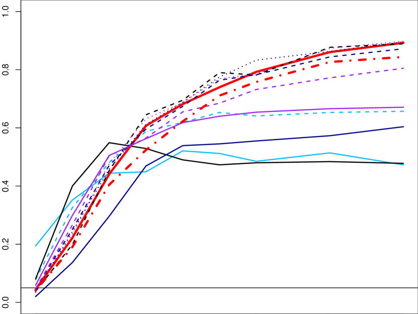
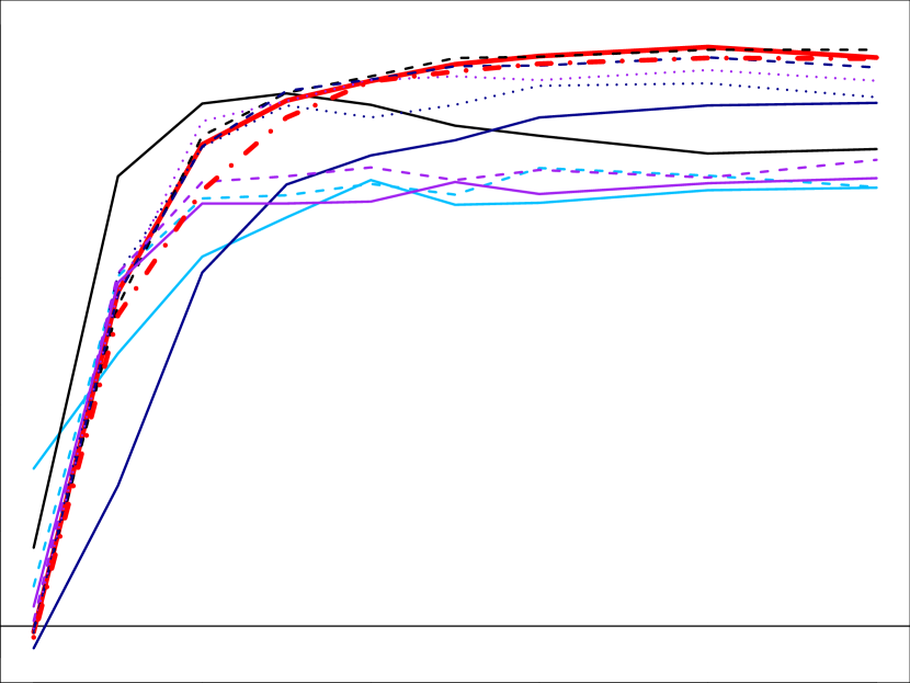
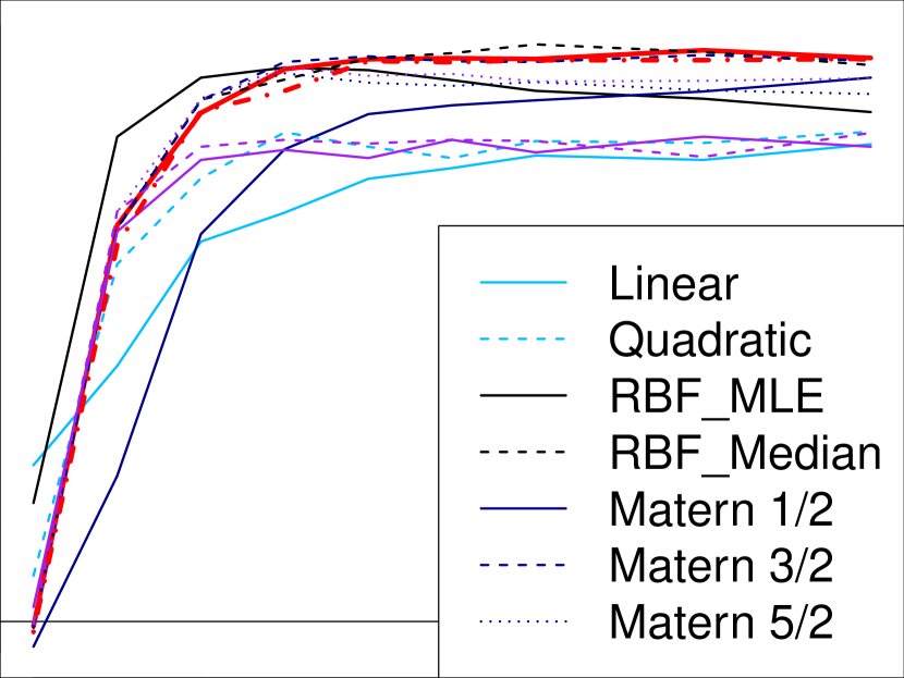
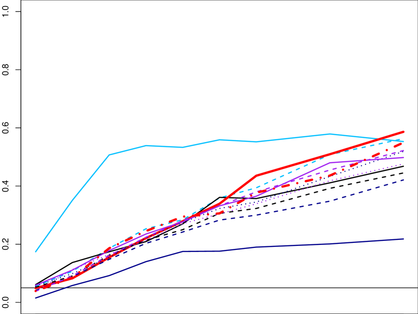
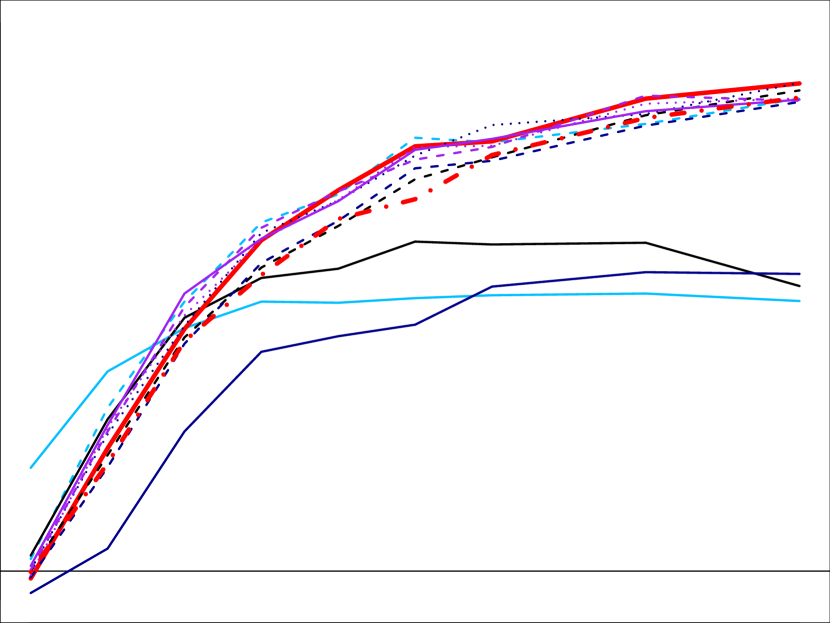
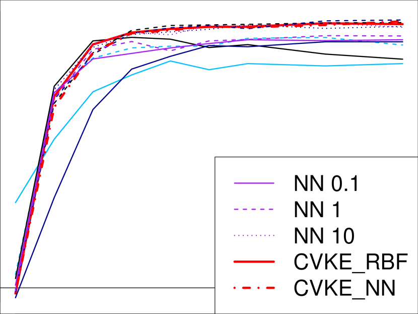
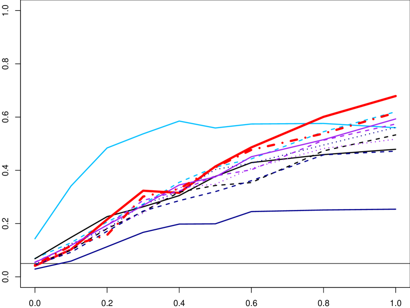
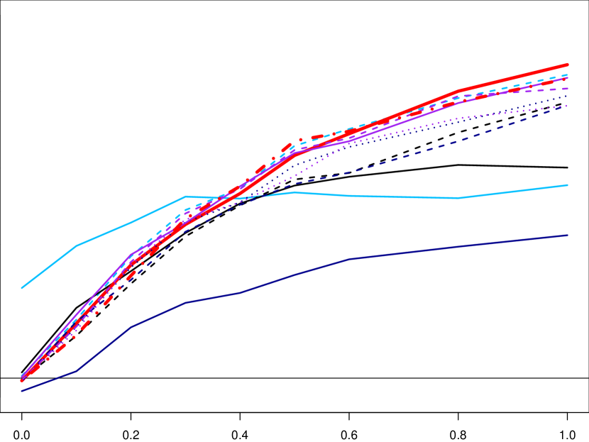
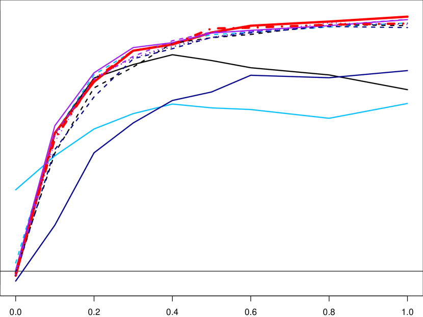
Skype Blue: Linear (Solid) and Quadratic (Dashed) Kernels, Black: RBF-Median (Solid) and RBF-MLE (Dashed), Dark Blue: Matérn Kernels with , Purple: Neural Network Kernels with , Red: CVEK based on RBF (Solid) and Neural Networks (Dashed).
Horizontal line marks the test’s significance level (0.05). When , should be below this line.
References
- [1] N. Aronszajn. Theory of reproducing kernels. Transactions of the American Mathematical Society, 68(3):337–404, 1950.
- [2] C. Cortes, M. Mohri, and A. Rostamizadeh. Two-Stage Learning Kernel Algorithms. 2010.
- [3] C. Cortes, M. Mohri, and A. Rostamizadeh. Ensembles of Kernel Predictors. arXiv:1202.3712 [cs, stat], Feb. 2012. arXiv: 1202.3712.
- [4] A. Davies and Z. Ghahramani. The Random Forest Kernel and other kernels for big data from random partitions. arXiv:1402.4293 [cs, stat], Feb. 2014. arXiv: 1402.4293.
- [5] A. Elisseeff and M. Pontil. Leave-one-out Error and Stability of Learning Algorithms with Applications. In J. Suykens, G. Horvath, S. Basu, C. Micchelli, and J. Vandewalle, editors, Learning Theory and Practice. IOS Press, 2002.
- [6] T. Evgeniou, L. Perez-Breva, M. Pontil, and T. Poggio. Bounds on the Generalization Performance of Kernel Machine Ensembles. In Proceedings of the Seventeenth International Conference on Machine Learning, ICML ’00, pages 271–278, San Francisco, CA, USA, 2000. Morgan Kaufmann Publishers Inc.
- [7] T. Evgeniou, M. Pontil, and A. Elisseeff. Leave One Out Error, Stability, and Generalization of Voting Combinations of Classifiers. Machine Learning, 55(1):71–97, Apr. 2004.
- [8] C. Gu. Smoothing Spline ANOVA Models. Springer Science & Business Media, Jan. 2013. Google-Books-ID: 5VxGAAAAQBAJ.
- [9] D. A. Harville. Maximum Likelihood Approaches to Variance Component Estimation and to Related Problems. Journal of the American Statistical Association, 72(358):320–338, 1977.
- [10] K. Hornik. Approximation capabilities of multilayer feedforward networks. Neural Networks, 4(2):251–257, 1991.
- [11] X. Lin. Variance component testing in generalised linear models with random effects. Biometrika, 84(2):309–326, June 1997.
- [12] D. Liu, X. Lin, and D. Ghosh. Semiparametric Regression of Multidimensional Genetic Pathway Data: Least-Squares Kernel Machines and Linear Mixed Models. Biometrics, 63(4):1079–1088, Dec. 2007.
- [13] A. Maity and X. Lin. Powerful tests for detecting a gene effect in the presence of possible gene-gene interactions using garrote kernel machines. Biometrics, 67(4):1271–1284, Dec. 2011.
- [14] C. E. Rasmussen and C. K. I. Williams. Gaussian Processes for Machine Learning. University Press Group Limited, Jan. 2006. Google-Books-ID: vWtwQgAACAAJ.
- [15] J. Snoek, H. Larochelle, and R. P. Adams. Practical Bayesian Optimization of Machine Learning Algorithms. arXiv:1206.2944 [cs, stat], June 2012. arXiv: 1206.2944.
- [16] G. Wahba. Spline Models for Observational Data. SIAM, Sept. 1990. Google-Books-ID: ScRQJEETs0EC.
- [17] A. G. Wilson, Z. Hu, R. Salakhutdinov, and E. P. Xing. Deep Kernel Learning. arXiv:1511.02222 [cs, stat], Nov. 2015. arXiv: 1511.02222.
- [18] D. Zhang and X. Lin. Hypothesis testing in semiparametric additive mixed models. Biostatistics (Oxford, England), 4(1):57–74, Jan. 2003.