Strong convergence of the linear implicit Euler method for the finite element discretization of semilinear SPDEs driven by multiplicative or additive noise

Abstract

This paper aims to investigate the numerical approximation of a general second order parabolic stochastic partial differential equation(SPDE) driven by multiplicative or additive noise. The linear operator is not necessary self-adjoint, so more useful in concrete applications. The SPDE is discretized in space by the finite element method and in time by the linear implicit Euler method. The corresponding scheme is more stable and efficient to solve stochastic advection-dominated reactive transport in porous media. This extends the current results in the literature to not necessary self-adjoint operator. As a challenge, key part of the proof does not rely anymore on the spectral decomposition of the linear operator. The results reveal how the convergence orders depend on the regularity of the noise and the initial data. In particular for multiplicative trace class noise, we achieve optimal convergence order $\mathcal{O}(h^{2}+\Delta t^{1/2})$ and for additive trace class noise, we achieve optimal convergence order in space and sup-optimal convergence order in time of the form $\mathcal{O}(h^{2}+\Delta t^{1-\epsilon})$, for an arbitrarily small $\epsilon>0$. Numerical experiments to sustain our theoretical results are provided.

1 Introduction

We consider numerical approximation of SPDE defined in $\Lambda\subset\mathbb{R}^{d}$, $d=1,2,3$, with initial value and boundary conditions (Dirichlet, Neumann or Robin boundary conditions). We consider the parabolic SPDE of the form

$$dX(t)+AX(t)dt=F(X(t))dt+B(X(t))dW(t),\quad X(0)=X_{0},\quad t\in(0,T]$$ (1)

on the Hilbert space $L^{2}(\Lambda)$. We denote by $T>0$ the final time, $F$ and $B$ are nonlinear functions, $X_{0}$ is the initial data which is random, $A$ is a linear operator, unbounded, not necessarily self-adjoint, and $-A$ is assumed to be a generator of an analytic semigroup $S(t)=:e^{-tA}$, $t\geq 0.$ The noise $W(t)=W(x,t)$ is a $Q$-Wiener process defined in a filtered probability space $\left(\Omega,\mathcal{F},\mathbb{P},\{\mathcal{F}_{t}\}_{t\geq 0}\right)$. The filtration is assumed to fulfill the usual conditions (see [20, Definition 2.1.11]). It is well known that the noise can be represented as follows

$$W(x,t)=\sum_{i\in\mathbb{N}^{d}}\sqrt{q_{i}}e_{i}(x)\beta_{i}(t),\quad t\in[0,T],$$ (2)

where $q_{i}$, $e_{i}$, $i\in\mathbb{N}^{d}$ are respectively the eigenvalues and the eigenfunctions of the covariance operator $Q$, and $\beta_{i}$ are independent and identically distributed standard Brownian motions. Precise assumptions on $F$, $B$, $X_{0}$ and $A$ will be given in the next section to ensure the existence of the unique mild solution $X$ of (1), which has the following representation (see [18, 20])

$$X(t)=S(t)X_{0}+\int_{0}^{t}S(t-s)F(X(s))ds+\int_{0}^{t}S(t-s)B(X(s))dW(s),\quad t\in(0,T].$$ (3)

Equations of type (1) are used to model different real world phenomena in different fields such as biology, chemistry, physics etc [21, 22, 4]. In more cases explicit solutions of SPDEs are unknown, therefore numerical methods are powerful tools appropriated for their approximations. Numerical approximation of SPDE of type (1) is therefore an active research area and have attracted a lot of attentions since two decades, see e.g., [15, 27, 28, 11, 6, 7, 30, 29, 21, 19, 9] and references therein. Due to the time step restriction of the explicit Euler method, linear implicit Euler method is used in many situations. Linear implicit Euler method have been investigated in the literature, see e.g., [11, 28, 16]. The work in [16] deals with the case of additive noise with self-ajoint operator and uses the spectral Galerkin method for the space discretization while the work in [11] still deals with self-adjoint operator, multiplicative noise and uses the standard finite element method for space discretization. The work in [28] considers the case of additive noise with self-adjoint operator and also uses finite element method for space dicretization. Note that the proofs of the results in [11, 28, 16] are heavily based on the spectral decomposition of the unbounded linear operator $A$, see e.g., [11, Lemma 4.4, Lemma 4.3, Lemma 4.2 & Lemma 4.1]. In fact, the proof of [11, Lemma 4.1] and [11, Lemma 4.2] use respectively [26, Theorem 3.4] and [26, Theorem 3.3], which are based on the self-adjoint assumption [26, (i), Page 40, Chapter 3]. Note also that that the proof of [11, Lemma 4.3 (i)-(ii)] rely on [26, Theorem 7.7 & Theorem 7.8], which is based on the spectral decomposition. More precisely, the proof of [26, Theorem 7.7 & Theorem 7.8] are based on [26, Theorem 7.2 & Theorem 7.3], which use the spectral decomposition. The proof of [11, Lemma 4.3 (iii)] also uses the spectral decomposition. The proof of the results in [28] are also strongly based on [26, Theorem 7.7 & Theorem 7.8] and some preparatory results for self adjoint operator in [11]. Therefore results in [11, 28, 16] cannot be easily extended to the case of non self-adjoint operator. Our aim in this work is to fill that gap and investigate the case of not necessary self-adjoint operator, more useful in concrete applications, which has not yet been investigated in the literature to best of our knowledge. Note that although the work in [11] solves general second order stochastic parabolic PDEs considered here by adding the advection term on nonlinear function $F$, the linear implicit Euler method in such approach behaves as the unstable explicit Euler method for strong advection term. An illustrative example is the stochastic dominated transport flow in porous media with high Péclet number [4]. In such cases, to stablilize the implicit scheme, it is important to include the advection term in the linear operator, which is treated implicitly in the linear implicit method, but current works in [11, 28, 16] are not longer applicable since the linear operator is not longer self-adjoint. Our goal here is to fill this gap and provide strong convergence results for multiplicative and additive noise for SPDE with not necessary self-adjoint operator. Note that numerical schemes for problem (1) with not necessary self-adjoint operator $A$ have been performed in [15, 17] for exponential integrators. Since solving linear systems are more straightforward than computing the exponential of matrix, it is important to develop alternative methods based on the resolution of linear systems, which may be more efficient if the appropriate preconditionners are used. The analysis of the linear implicit Euler scheme with not necessary self-adjoint operator is more difficult than those of an exponential schemes since the errors estimates in the corresponding determistic linear problem (Section 3.1) are extremely complex for non self-adjoint operator. Keys part of this work are based on those errors estimates with elegant properties of the semi-group and its approximation, in opposite of the spectral decomposition currently used in the literature [11, 28]. The results indicate how the convergence orders depend on the regularity of the initial data and the noise. In particular, we achieve the optimal convergence orders $\mathcal{O}\left(h^{\beta}+\Delta t^{\min(\beta,1)/2}\right)$ for multiplicative noise; the optimal convergence order in space and sup-optimal convergence order in time of the form $\mathcal{O}\left(h^{\beta}+\Delta t^{\min({\beta/2},1-\epsilon)}\right)$ for additive noise, where $\beta$ is the regularity’s parameter of the noise (see Assumption 2.1) and $\epsilon>0$ is an arbitrarily real number small enough. It is worth to mention that these optimal convergence orders were also achieved in [11, 28] with self-adjoint operator, where the convergence analysis was heavily based on the spectral decomposition of the linear operator $A$.

The rest of this paper is organized as follows. Section 2 deals with the well posedness problem, the numerical scheme and the main results. In section 3, we first provide some error estimates for the deterministic homogeneous problem as preparatory results and we provide the proof of the main results. Section 4 provides some numerical experiments to sustain the theoretical results.

2 Mathematical setting and main results

2.1 Setting and assumptions

Let us define functional spaces, norms and notations that will be used in the rest of the paper. Let $(H,\langle.,.\rangle_{H},\|.\|)$ be a separable Hilbert space. For $p\geq 2$ and for a Banach space $U$, we denote by $L^{p}(\Omega,U)$ the Banach space of all equivalence classes of $p$ integrable $U$-valued random variables. We denote by $L(U,H)$ the space of bounded linear mappings from $U$ to $H$ endowed with the usual operator norm $\|.\|_{L(U,H)}$. By $\mathcal{L}_{2}(U,H):=HS(U,H)$, we denote the space of Hilbert-Schmidt operators from $U$ to $H$. We equip $\mathcal{L}_{2}(U,H)$ with the norm

$$\|l\|^{2}_{\mathcal{L}_{2}(U,H)}:=\sum_{i=1}^{\infty}\|l\psi_{i}\|^{2},\quad l\in\mathcal{L}_{2}(U,H),$$ (4)

where $(\psi_{i})_{i=1}^{\infty}$ is an orthonormal basis of $U$. Note that (4) is independent of the orthonormal basis of $U$. For simplicity we use the notations $L(U,U)=:L(U)$ and $\mathcal{L}_{2}(U,U)=:\mathcal{L}_{2}(U)$. It is well known that for all $l\in L(U,H)$ and $l_{1}\in\mathcal{L}_{2}(U)$, $ll_{1}\in\mathcal{L}_{2}(U,H)$ and

$$\|ll_{1}\|_{\mathcal{L}_{2}(U,H)}\leq\|l\|_{L(U,H)}\|l_{1}\|_{\mathcal{L}_{2}(U)}.$$ (5)

We assume that the covariance operator $Q:H\longrightarrow H$ is positive and self-adjoint. The space of Hilbert-Schmidt operators from $Q^{1/2}(H)$ to $H$ is denoted by $L^{0}_{2}:=\mathcal{L}_{2}(Q^{1/2}(H),H)=HS(Q^{1/2}(H),H)$ with the corresponding norm $\|.\|_{L^{0}_{2}}$ defined by

$$\|l\|_{L^{0}_{2}}:=\|lQ^{1/2}\|_{HS}=\left(\sum_{i=1}^{\infty}\|lQ^{1/2}e_{i}\|^{2}\right)^{1/2},\quad l\in L^{0}_{2},$$ (6)

where $(e_{i})_{i=1}^{\infty}$ is an orthonormal basis of $H$. Note that (6) is independent of the orthonormal basis of $H$. In the rest of this paper, we take $H=L^{2}(\Lambda)$.

Throughout this paper, we assume that $\Lambda$ is bounded and has smooth boundary or is a convex polygon of $\mathbb{R}^{d}$, $d=1,2,3$. In the rest of this paper we consider the SPDE (1) to be of the following form

$$dX(t,x)+[-\nabla\cdot\left(\mathbf{D}\nabla X(t,x)\right)+\mathbf{q}\cdot\nabla X(t,x)]dt=f(x,X(t,x))dt+b(x,X(t,x))dW(t,x),$$ (7)

$x\in\Lambda$, $t\in[0,T]$, where the function $f:\Lambda\times\mathbb{R}\longrightarrow\mathbb{R}$ is continuously twice differentiable and the function $b:\Lambda\times\mathbb{R}\longrightarrow\mathbb{R}$ is continuously differentiable with globally bounded derivatives. In the abstract framework (1), the linear operator $A$ takes the form

$$Au=-\sum_{i,j=1}^{d}\dfrac{\partial}{\partial x_{i}}\left(D_{ij}(x)\dfrac{\partial u}{\partial x_{j}}\right)+\sum_{i=1}^{d}q_{i}(x)\dfrac{\partial u}{\partial x_{i}},\quad\mathbf{D}=\left(D_{i,j}\right)_{1\leq i,j\leq d},\,\,\,\,\,\,\,\mathbf{q}=\left(q_{i}\right)_{1\leq i\leq d}.$$ (8)

where $D_{ij}\in L^{\infty}(\Lambda)$, $q_{i}\in L^{\infty}(\Lambda)$. We assume that there exists a constant $c_{1}>0$ such that

$$\sum_{i,j=1}^{d}D_{ij}(x)\xi_{i}\xi_{j}\geq c_{1}|\xi|^{2},\quad\forall\xi\in\mathbb{R}^{d},\quad x\in\overline{\Omega}.$$ (9)

The functions $F:H\longrightarrow H$ and $B:H\longrightarrow HS\left(Q^{1/2}(H),H\right)$ are defined by

$$\left(F(v)\right)(x)=f\left(x,v(x)\right)\quad\text{and}\quad\left(B(v)u\right)(x)=b\left(x,v(x)\right).u(x),$$ (10)

for all $x\in\Lambda$, $v\in H$, $u\in Q^{1/2}(H)$, with $H=L^{2}(\Lambda)$. For an appropriate family of eigenfunctions $(e_{i})$ such that $\sup\limits_{i\in\mathbb{N}^{d}}\left[\sup\limits_{x\in\Lambda}\|e_{i}(x)\|\right]<\infty$, it is well known [8, Section 4] that the Nemytskii operator $F$ related to $f$ and the multiplication operator $B$ associated to $b$ defined in (10) satisfy Assumption 2.2, Assumption 2.3 and Assumption 2.4. As in [15, 3] we introduce two spaces $\mathbb{H}$ and $V$, such that $\mathbb{H}\subset V$; the two spaces depend on the boundary conditions and the domain of the operator $A$. For Dirichlet (or first-type) boundary conditions we take

$$V=\mathbb{H}=H^{1}_{0}(\Lambda)=\overline{C^{\infty}_{c}(\Lambda)}^{H^{1}(\Lambda)}=\{v\in H^{1}(\Lambda):v=0\quad\text{on}\quad\partial\Lambda\}.$$

For Robin (third-type) boundary condition and Neumann (second-type) boundary condition, which is a special case of Robin boundary condition, we take $V=H^{1}(\Lambda)$

$$\mathbb{H}=\{v\in H^{2}(\Lambda):\partial v/\partial\mathtt{v}_{A}+\alpha_{0}v=0,\quad\text{on}\quad\partial\Lambda\},\quad\alpha_{0}\in\mathbb{R},$$

where $\partial v/\partial\mathtt{v}_{A}$ is the normal derivative of $v$ and $\mathtt{v}_{A}$ is the exterior pointing normal at $n=(n_{i})$ to the boundary of $A$, given by

$$\partial v/\partial\mathtt{v}_{A}=\sum_{i,j=1}^{d}n_{i}(x)D_{ij}(x)\dfrac{\partial v}{\partial x_{j}},\,\,\qquad x\in\partial\Lambda.$$

Using the Green’s formula and the boundary conditions, the corresponding bilinear form associated to $A$ is given by

$$a(u,v)=\int_{\Lambda}\left(\sum_{i,j=1}^{d}D_{ij}\dfrac{\partial u}{\partial x_{i}}\dfrac{\partial v}{\partial x_{j}}+\sum_{i=1}^{d}q_{i}\dfrac{\partial u}{\partial x_{i}}v\right)dx,\quad u,v\in V,$$

for Dirichlet and Neumann boundary conditions, and

$$a(u,v)=\int_{\Lambda}\left(\sum_{i,j=1}^{d}D_{ij}\dfrac{\partial u}{\partial x_{i}}\dfrac{\partial v}{\partial x_{j}}+\sum_{i=1}^{d}q_{i}\dfrac{\partial u}{\partial x_{i}}v\right)dx+\int_{\partial\Lambda}\alpha_{0}uvdx,\quad u,v\in V,$$

for Robin boundary conditions. Using the Gårding’s inequality (see e.g. [22]), it holds that there exist two constants $c_{0}$ and $\lambda_{0}\geq 0$ such that

$$a(v,v)\geq\lambda_{0}\|v\|^{2}_{H^{1}(\Lambda)}-c_{0}\|v\|^{2},\quad v\in V.$$ (11)

By adding and substracting $c_{0}Xdt$ in both sides of (1), we have a new linear operator still denoted by $A$, and the corresponding bilinear form is also still denoted by $a$. Therefore, the following coercivity property holds

$$a(v,v)\geq\lambda_{0}\|v\|^{2}_{1},\quad v\in V.$$ (12)

Note that the expression of the nonlinear term $F$ has changed as we included the term $c_{0}X$ in a new nonlinear term that we still denote by $F$. The coercivity property (12) implies that $-A$ is sectorial in $L^{2}(\Lambda)$, i.e. there exist $C_{1},\,\theta\in(\frac{1}{2}\pi,\pi)$ such that

$$\|(\lambda I+A)^{-1}\|_{L(L^{2}(\Lambda))}\leq\dfrac{C_{1}}{|\lambda|},\;\quad\quad\lambda\in S_{\theta},$$

where $S_{\theta}=\left\{\lambda\in\mathbb{C}:\lambda=\rho e^{i\phi},\;\rho>0,\;0\leq|\phi|\leq\theta\right\}$ (see [5]). Then $-A$ is the infinitesimal generator of a bounded analytic semigroup $S(t)=e^{-tA}$ on $L^{2}(\Lambda)$ such that

$$S(t)=e^{-tA}=\dfrac{1}{2\pi i}\int_{\mathcal{C}}e^{t\lambda}(\lambda I+A)^{-1}d\lambda,\;\;\;\;\;\;\;\;t>0,$$

where $\mathcal{C}$ denotes a path that surrounds the spectrum of $-A$. The coercivity property (12) also implies that $A$ is a positive operator and its fractional powers are well defined for any $\alpha>0,$ by

$$\left\{\begin{array}[]{rcl}A^{-\alpha}&=&\frac{1}{\Gamma(\alpha)}\displaystyle\int_{0}^{\infty}t^{\alpha-1}{\rm e}^{-tA}dt,\\ A^{\alpha}&=&(A^{-\alpha})^{-1},\end{array}\right.$$ (13)

where $\Gamma(\alpha)$ is the Gamma function (see [5]).

Under condition (9), it is well known (see e.g. [3]) that the linear operator $-A$ given by (8) generates an analytic semigroup $S(t)\equiv e^{-tA}$. Following [1, 14, 15, 3], we characterize the domain of the operator $A^{r/2}$ denoted by $\mathcal{D}(A^{r/2})$, $r\in\{1,2\}$ with the following equivalence of norms, useful in our convergence proofs

$$\|v\|_{H^{1}(\Lambda)}\equiv\|A^{r/2}v\|=:\|v\|_{r},\quad v\in\mathcal{D}(A^{r/2}),$$

$$\mathcal{D}(A^{r/2})=\mathbb{H}\cap H^{r}(\Lambda),\quad\text{ (for Dirichlet boundary conditions)},$$

$$\mathcal{D}(A)=\mathbb{H},\quad\mathcal{D}(A^{1/2})=H^{1}(\Lambda),\quad\text{(for Robin boundary conditions)}.$$

Remark 2.1

For Dirichlet boundary conditions, if $\bigtriangledown\cdot\mathbf{q}=0$, as we can see in [24], the coercivity (12) is obtained with $c_{0}=0$, and Gårding’s inequality is not needed. We can aslo notice from [24] that the constant $c_{0}$ depends only on $\bigtriangledown\cdot\mathbf{q}$. Indeed for $\mathbf{q}$ smooth enough, $\mathbf{q}\cdot\nabla X=\nabla\cdot(\mathbf{q}X)-(\bigtriangledown\cdot\mathbf{q})X$, so adding and subtracting $c_{0}Xdt$ in both sides of (1), should in many realistic cases always weaken the advection term even for strong divergence flow ($c_{0}$ large), and therefore stabilize the semi implicit scheme more than the work in [11] where the whole advection term is kept in the nonlinear function $F$.

In order to ensure the existence and the uniqueness of solution for SPDE (1) and for the purpose of the convergence analysis, we make the following assumptions.

Assumption 2.1

[Initial value $X_{0}$] Let $p\in[2,\infty)$. We assume that the initial data $X_{0}$ belongs to $L^{p}(\Omega,\mathcal{D}((-A)^{\beta/2}))$, $0<\beta\leq 2$.

Assumption 2.2

[Nonlinear term $F$] The nonlinear function $F:H\longrightarrow H$ is Lipschitz continuous, i.e. there exists a constant $C>0$ such that

$$\|F(0)\|\leq C,\quad\|F(Y)-F(Z)\|\leq C\|Y-Z\|,\quad Y,Z\in H.$$ (14)

As a consequence of (14), it holds that

$$\|F(Z)\|\leq C(1+\|Z\|),\quad Z\in H.$$

Following [18, Chapter 7] or [29, 15, 8, 11], we make the following assumption on the diffusion term.

Assumption 2.3

[Diffusion term ] We assume that the operator $B:H\longrightarrow L^{0}_{2}$ satisfies the global Lipschitz condition, i.e. there exists a positive constant $C$ such that

$$\|B(0)\|_{L^{0}_{2}}\leq C,\quad\|B(Y)-B(Z)\|_{L_{2}^{0}}\leq C\|Y-Z\|,\quad Y,Z\in H.$$

As a consequence, it holds that

$$\|B(Z)\|_{L^{0}_{2}}\leq L(1+\|Z\|),\quad Z\in H.$$

We equip $V_{\alpha}:=\mathcal{D}(A^{\alpha/2})$, $\alpha\in\mathbb{R}$ with the norm $\|v\|_{\alpha}:=\|A^{\alpha/2}v\|$, for all $v\in H$. It is well known that $(V_{\alpha},\|.\|_{\alpha})$ is a Banach space [5].

To establish our $L^{p}$ strong convergence result when dealing with multiplicative noise, we will also need the following further assumption on the diffusion term when $\beta\in[1,2]$, which was also used in [8, 12] to achieve optimal order regularity and in [15, 11, 17] to achieve optimal convergence order in space and time.

Assumption 2.4

There exists a positive constant $c>0$ such that $B\left(\mathcal{D}\left(A^{(\beta-1)/2}\right)\right)\subset HS\left(Q^{1/2}(H),\mathcal{D}\left(A^{(\beta-1)/2}\right)\right)$ and $\left\|A^{(\beta-1)/2}B(v)\right\|_{L^{0}_{2}}\leq c\left(1+\|v\|_{\beta-1}\right)$ for all $v\in\mathcal{D}\left(A^{(\beta-1)/2}\right)$, where $\beta$ comes from Assumption 2.1.

Typical examples which fulfill Assumption 2.4 are stochastic reaction diffusion equations (see [8, Section 4]).

When dealing with additive noise (i.e. when the nonlinear function $B$ is independent of $X$), the strong convergence proof will make use of the following assumption, also used in [28, 27, 17].

Assumption 2.5

We assume that the covariance operator $Q$ satisfy the following estimate

$$\left\|A^{\frac{\beta-1}{2}}Q^{\frac{1}{2}}\right\|_{\mathcal{L}_{2}(H)}<C,$$

where $\beta$ comes from Assumption 2.1.

When dealing with additive noise, to achieve higher order convergence in time, we assume the nonlinear function to satisfy the following assumption, also used in [27, 28, 17].

Assumption 2.6

The deterministic mapping $F:H\longrightarrow H$ is twice differentiable and there exist constants $L\geq 0$ and $\eta\in[0,1)$ such that

$$\|F^{\prime}(u)v\|\leq L\|v\|,\quad\|F^{\prime\prime}(u)(v_{1},v_{2})\|_{-\eta}\leq L\|v_{1}\|.\|v_{2}\|,\quad u,v,v_{1},v_{2}\in H.$$ (15)

Let us recall the following proposition which provides some smooth properties of the semigroup $S(t)$ generated by $-A$, that will be useful in the rest of the paper.

Proposition 2.1

[Smoothing properties of the semigroup][5] Let $\alpha>0$, $\delta\geq 0$ and $0\leq\gamma\leq 1$, then there exists a constant $C>0$ such that

$$\|A^{\delta}S(t)\|_{L(H)}\leq Ct^{-\delta},\quad t>0,\quad\|A^{-\gamma}\left(\mathbf{I}-S(t)\right)\|_{L(H)}\leq Ct^{\gamma},\quad t\geq 0$$

$$A^{\delta}S(t)=S(t)A^{\delta},\quad\text{on}\quad\mathcal{D}(A^{\delta}),\quad\|D^{l}_{t}S(t)v\|_{\delta}\leq Ct^{-l-(\delta-\alpha)/2}\|v\|_{\alpha},\quad t>0,\quad v\in\mathcal{D}(A^{\alpha}),$$

where $l=0,1$, and $D^{l}_{t}=\dfrac{d^{l}}{dt^{l}}$. If $\delta\geq\gamma$ then $\mathcal{D}(A^{\delta})\subset\mathcal{D}(A^{\gamma})$.

Theorem 2.1

[18, Theorem 7.2]
Let Assumption 2.2 and Assumption 2.3 be satisfied. If $X_{0}$ is a $\mathcal{F}_{0}$- measurable $H$ valued random variable, then there exists a unique mild solution $X$ of the problem (1) represented by (3) and satisfying

$$\mathbb{P}\left[\int_{0}^{T}\|X(s)\|^{2}ds<\infty\right]=1,$$

and for any $p\geq 2$, there exists a constant $C=C(p,T)>0$ such that

$$\sup_{t\in[0,T]}\mathbb{E}\|X(t)\|^{p}\leq C(1+\mathbb{E}\|X_{0}\|^{p}).$$

2.2 Fully discrete scheme and main results

Let us start with the space discretization of our problem (1). We start by splitting the domain $\Lambda$ in finite triangles. Let $\mathcal{T}_{h}$ be the triangulation with maximal length $h$ satisfying the usual regularity assumptions, and $V_{h}\subset V$ be the space of continuous functions that are piecewise linear over the triangulation $\mathcal{T}_{h}$. We consider the projection $P_{h}$ from $H=L^{2}(\Lambda)$ to $V_{h}$ defined by

$$\langle P_{h}u,\chi\rangle_{H}=\langle u,\chi\rangle_{H},\quad u\in H,\quad\chi\in V_{h}.$$ (16)

The discrete operator $A_{h}:V_{h}\longrightarrow V_{h}$ is defined by

$$\langle A_{h}\phi,\chi\rangle_{H}=\langle A\phi,\chi\rangle_{H}=a(\phi,\chi),\quad\phi,\chi\in V_{h},$$ (17)

Like $-A$, $-A_{h}$ is also a generator of an analytic semigroup $S_{h}(t)=:e^{-tA_{h}}$, see e.g. [14, 3]. As any analytic semigroup and their generator, $-A_{h}$ and $S_{h}(t)$ satisfy the smoothing properties of Proposition 2.1 with a uniform constant $C$ (i.e. independent of $h$), see e.g. [14, 3]. The semi-discrete version of problem (1) consists of finding $X^{h}(t)\in V_{h}$, $t\in(0,T]$ such that

$$dX^{h}(t)+A_{h}X^{h}(t)dt=P_{h}F(X^{h}(t))dt+P_{h}B(X^{h}(t))dW(t),\quad X^{h}(0)=P_{h}X_{0},\quad t\in(0,T].$$ (18)

Applying the linear implict Euler method to (18) gives the following fully discrete scheme

$$\left\{\begin{array}[]{ll}X^{h}_{0}=P_{h}X_{0},\\ X^{h}_{m+1}=S_{h,\Delta t}X^{h}_{m}+\Delta tS_{h,\Delta t}P_{h}F(X^{h}_{m})+S_{h,\Delta t}P_{h}B(X^{h}_{m})\Delta W_{m},\end{array}\right.$$ (21)

where $\Delta W_{m}$ and $S_{h,\Delta t}$ are defined respectively by

$$\Delta W_{m}:=W_{t_{m+1}}-W_{t_{m}}\quad\text{and}\quad S_{h,\Delta t}:=(\mathbf{I}+\Delta tA_{h})^{-1}.$$ (22)

Having the numerical method (21) in hand, our goal is to analyze its strong convergence toward the exact solution in the $L^{p}$ norm for multiplicative and additive noise.

Throughout this paper we take $t_{m}=m\Delta t\in[0,T]$, where $T=M\Delta t$ for $m,M\in\mathbb{N}$, $m\leq M$, $T$ is fixed, $C$ is a generic constant that may change from one place to another. The main results of this paper are formulated in the following theorems.

Theorem 2.2

Let $X(t_{m})$ and $X^{h}_{m}$ be respectively the mild solution given by (3) and the numerical approximation given by (21) at $t_{m}=m\Delta t$. Let Assumptions 2.1, 2.2 and 2.3 be fulfilled.

• If $0<\beta<1$, then the following error estimate holds

  $$\|X(t_{m})-X^{h}_{m}\|_{L^{p}(\Omega,H)}\leq C\left(h^{\beta}+\Delta t^{\beta/2}\right).$$

• If $1\leq\beta\leq 2$ and if Assumption 2.4 is fulfilled, then the following error estimate holds

  $$\|X(t_{m})-X^{h}_{m}\|_{L^{p}(\Omega,H)}\leq C\left(h^{\beta}+\Delta t^{1/2}\right).$$

For additive noise, we have the following convergence result.

Theorem 2.3

In the case of additive noise, if Assumptions 2.1, 2.2, 2.5 with $\beta\in[0,2)$ and Assumption 2.6 are fulfilled, then the following error estimate holds for the mild solution $X(t)$ of (1) and the numerical approximation (21)

$$\|X(t_{m})-X^{h}_{m}\|_{L^{p}(\Omega,H)}\leq C\left(h^{\beta}+\Delta t^{\beta/2}\right).$$

Moreover, if Assumptions 2.5 and 2.1 are fulfilled with $\beta=2$, then the following holds

$$\|X(t_{m})-X^{h}_{m}\|_{L^{p}(\Omega,H)}\leq C\left(h^{\beta}+\Delta t^{1-\epsilon}\right),$$

for an arbitrarily small $\epsilon>0$.

3 Proof of the main results

The proof of the main results requires some preparatory results.

3.1 Errors estimates for deterministic problem

This section extends results in [11, Section 4], [28, Section 3] and some results in [26] to the case of not necessary self-adjoint operator. As we are dealing with not necessary self-adjoint operator, the proof of our estimates does not make use of the spectral decomposition of the linear operator $A$. Let us start by introducing the Ritz representation operator $R_{h}:V\longrightarrow V_{h}$ defined by

$$\langle AR_{h}v,\chi\rangle_{H}=\langle Av,\chi\rangle_{H}=a(v,\chi),\quad v\in V,\quad\chi\in V_{h}.$$ (23)

Under the regularity assumptions on the triangulation and in view of the $V$-ellipticity (9), it is well known (see e.g. [3, 14]) that for all $r\in\{1,2\}$ the following error estimates hold

$$\|R_{h}v-v\|+h\|R_{h}v-v\|_{H^{1}(\Lambda)}\leq Ch^{r}\|v\|_{H^{r}(\Lambda)},\quad v\in V\cap H^{r}(\Lambda).$$ (24)

Let us consider the following deterministic linear problem : Find $u\in V$ such that

$$\dfrac{du}{dt}+Au=0,\quad u(0)=v,\quad t\in(0,T].$$ (25)

The corresponding semi-discrete problem in space consists of finding $u_{h}\in V_{h}$ such that

$$\dfrac{du_{h}}{dt}+A_{h}u_{h}=0,\quad u_{h}(0)=P_{h}v,\quad t\in(0,T].$$ (26)

Let us define the following operator

$$G_{h}(t):=S(t)-S_{h}(t)P_{h}=e^{-At}-e^{-A_{h}t}P_{h},$$

so that $u(t)-u_{h}(t)=G_{h}(t)v$. The estimate (24) was used in [15, 17] to prove the following lemma, with the prove available in [15, Lemma 3.1] or [17, Lemma 7].

Lemma 3.1

Under the setting in Section 2.1, the following estimate holds

$$\|G_{h}(t)v\|\leq Ch^{r}t^{-(r-\alpha)/2}\|v\|_{\alpha},\quad r\in[0,2],\quad\alpha\leq r,\,\,t\in(0,T].$$ (27)

Lemma 3.2

• Let $0\leq\rho\leq 1$. Then there exists a constant $C$ such that

  $$\|G_{h}(t)v\|\leq Ct^{-\rho/2}\|v\|_{-\rho},\quad v\in\mathcal{D}(A^{-\rho}),\quad t>0.$$ (28)

• Let $r\in[1,2]$, $1\leq\alpha\leq r$ and $v\in\mathcal{D}(A^{\alpha/2})$. Then there exists a constant $C\geq 0$ such that

  $$\|D_{t}(S(t)-S_{h}(t)P_{h})v\|\leq Ch^{\alpha}t^{-1}\|v\|_{\alpha}+Ch^{r}t^{-1-(r-\alpha)/2}\|v\|_{\alpha},$$

  for all $t>0$, where $D_{t}:=\frac{d}{dt}$.

• Let $0\leq\rho\leq 1$. Then there exists a constant $C$ such that

  $$\|G_{h}(t)v\|\leq Ch^{2-\rho}t^{-1}\|v\|_{-\rho},\quad v\in\mathcal{D}(A^{-\rho}),\quad t>0.$$ (29)

• Let $0\leq\rho\leq 1$. Then there exists a constant $C$ such that

  $$\left\|\int_{0}^{t}G_{h}(s)vds\right\|\leq Ch^{2-\rho}\|v\|_{-\rho},\quad v\in\mathcal{D}(A^{-\rho}),\quad t>0.$$ (30)

• Let $0\leq\gamma\leq 2$. Then the following estimate holds

  $$\left(\int_{0}^{t}\|G_{h}(s)v\|^{2}ds\right)^{1/2}\leq Ch^{\gamma}\|v\|_{\gamma-1},\quad v\in\mathcal{D}(A^{\gamma-1}),\quad t>0.$$

Proof.

• The proof of (i) is similar to [11, Lemma 4.1 (ii)] by using Lemma 3.2 instead of [11, Lemma 4.1 (i)].

• As in [15], we write

  $$u_{h}(t)-u(t)=(u_{h}(t)-R_{h}u(t))+(R_{h}u(t)-u(t))=:\theta(t)+\rho(t).$$ (31)

  Therefore the following estimate holds

  $$\|D_{t}(S(t)-S_{h}(t)P_{h})v\|\leq\|D_{t}\theta(t)\|+\|D_{t}\rho(t)\|.$$ (32)

  From [15], we have

  $$A_{h}R_{h}=P_{h}A,\quad\text{and}\quad\theta_{t}=A_{h}\theta(t)-P_{h}D_{t}\rho(t).$$ (33)

  Taking the derivative in both sides of the second expression of (33) and using the fact that $D_{t}P_{h}=P_{h}D_{t}$ (see e.g. [13, Page 16]), we obtain

  $$\theta_{tt}=A_{h}\theta_{t}-P_{h}D_{tt}\rho(t).$$ (34)

  Therefore, by Duhamel’s principle we have

  $$\theta_{t}(t)=S_{h}(t)\theta_{t}(0)-\int_{0}^{t}S_{h}(t-s)P_{h}D_{ss}\rho(s)ds.$$ (35)

  Splitting the integral part of (35) into two intervals and integrating by parts over the first interval yields

  $$\theta_{t}(t) = S_{h}(t)\theta_{t}(0)+S_{h}(t)P_{h}D_{t}\rho(0)-S_{h}(t/2)P_{h}D_{t}\rho(t/2)$$ (36)

  $$+ \int_{0}^{t/2}(D_{s}S_{h}(t-s))P_{h}D_{s}\rho(s)ds-\int_{t/2}^{t}S_{h}(t-s)P_{h}D_{ss}\rho(s)ds.$$

  From (33) it holds that $S_{h}(t)\theta_{t}(0)+S_{h}(t)P_{h}D_{t}\rho(0)=S_{h}(t)A_{h}\theta(0)$. Therefore (36) becomes

  $$\theta_{t}(t) = S_{h}(t)A_{h}\theta(0)-S_{h}(t/2)P_{h}D_{s}\rho(t/2)+\int_{0}^{t/2}(D_{s}S_{h}(t-s))P_{h}D_{s}\rho(s)ds$$ (37)

  $$- \int_{t/2}^{t}S_{h}(t-s)P_{h}D_{ss}\rho(s)ds.$$

  Taking the norm in both sides of (37), using the stability properties of the semigroup and the boundedness of $P_{h}$ yields

  $$\|\theta_{t}(t)\| \leq Ct^{-1}\|\theta(0)\|+C\|D_{t}\rho(t/2)\|+\left\|\int_{0}^{t/2}(D_{s}S_{h}(t-s))P_{h}D_{s}\rho(s)ds\right\|$$ (38)

  $$+ C\int_{t/2}^{t}\|D_{ss}\rho(s)\|ds.$$

  Using the definition of $\theta(t)$, the boundedness of $P_{h}$ and (24), it holds that

  $$\|\theta(0)\|=\|P_{h}v-R_{h}v\|=\|P_{h}v-P_{h}R_{h}v\|\leq\|v-R_{h}v\|\leq Ch^{\alpha}\|v\|_{\alpha}.$$ (39)

  Using (24) and Proposition 2.1 as in [15], we obtain

  $$\|D_{t}\rho(t)\|\leq Ch^{r}\|D_{t}u\|_{r}=Ch^{r}\|D_{t}S(t)v\|_{r}\leq Ch^{r}t^{-1-(r-\alpha)/2}\|v\|_{\alpha}.$$ (40)

  Using again (24) and Proposition 2.1, the following estimate holds

  $$\|D_{ss}\rho(s)\|\leq Ch^{r}\|D_{ss}u\|_{r}=Ch^{r}\|D_{ss}S(s)v\|_{r}\leq Ch^{r}s^{-2-(r-\alpha)/2}\|v\|_{\alpha}.$$ (41)

  Substituting (41), (40) and (39) in (38), it holds

  $$\|\theta_{t}(t)\|$$ (42)

  $$\leq Ch^{\alpha}t^{-1}\|v\|_{\alpha}+\left\|\int_{0}^{t/2}(D_{s}(S_{h}(t-s))P_{h}D_{s}\rho(s)ds\right\|+Ch^{r}\int_{t/2}^{t}s^{-2-(r-\alpha)/2}\|v\|_{\alpha}ds$$

  $$\leq Ch^{\alpha}t^{-1}\|v\|_{\alpha}+\left\|\int_{0}^{t/2}(D_{s}(S_{h}(t-s))P_{h}D_{s}\rho(s)ds\right\|+Ch^{r}t^{-1-(r-\alpha)/2}\|v\|_{\alpha}.$$

  Using the second relation of (33) and triangle inequality, it holds that

  $$\left\|\int_{0}^{t/2}\left(D_{s}S_{h}(t-s)\right)P_{h}D_{s}\rho(s)ds\right\|$$ (43)

  $$= \left\|\int_{0}^{t/2}\left(D_{s}S_{h}(t-s)\right)\left(A_{h}\theta(s)-\theta_{s}(s)\right)ds\right\|$$

  $$\leq \left\|\int_{0}^{t/2}\left(D^{2}_{s}(S_{h}(t-s)\right)\theta(s)ds\right\|+\left\|\int_{0}^{t/2}D_{s}S_{h}(t-s)\theta_{s}(s)ds\right\|.$$

  Note that

  $$D_{s}S_{h}(t-s)\theta_{s}(s)=D_{s}\left(D_{s}S_{h}(t-s)\theta(s)\right)-D^{2}_{s}S_{h}(t-s)\theta(s).$$ (44)

  Substituting (44) in (42) yields

  $$\left\|\int_{0}^{t/2}D_{s}S_{h}(t-s)\theta_{s}(s)ds\right\|$$ (45)

  $$\leq \left\|\int_{0}^{t/2}D_{s}\left(A_{h}S_{h}(t-s)\theta(s)\right)ds\right\|+\int_{0}^{t/2}\left\|D^{2}_{s}S_{h}(t-s)\theta(s)\right\|ds$$

  $$\leq \|A_{h}S_{h}(t/2)\theta(t/2)\|+\|A_{h}S_{h}(t)\theta(0)\|$$

  $$+ \int_{0}^{t/2}(t-s)^{-2}\|\theta(s)\|ds.$$

  We recall that from [15], we have the following estimate

  $$\|\theta(s)\|\leq Ch^{r}t^{-(r-\alpha)/2}\|v\|_{\alpha},\quad s>0.$$ (46)

  Substituting (46) and (39) in (45) and using the smooth properties of the semigroup yields

  $$\left\|\int_{0}^{t/2}D_{s}S_{h}(t-s)\theta(s)ds\right\|$$ (47)

  $$\leq Ch^{r}t^{-1-(r-\alpha)/2}\|v\|_{\alpha}+Ch^{\alpha}t^{-1}\|v\|_{\alpha}+C\int_{0}^{t/2}(t-s)^{-2}s^{-(r-\alpha)/2}\|v\|_{\alpha}ds$$

  $$\leq Ch^{r}t^{-1-(r-\alpha)/2}\|v\|_{\alpha}+Ch^{\alpha}t^{-1}\|v\|_{\alpha}+Ct^{-2}\int_{0}^{t/2}s^{-(r-\alpha)/2}\|v\|_{\alpha}ds$$

  $$\leq Ch^{r}t^{-1-(r-\alpha)/2}\|v\|_{\alpha}+Ch^{\alpha}t^{-1}\|v\|_{\alpha}.$$

  Using (46) and the stability property of the semigroup, it holds that

  $$\left\|\int_{0}^{t/2}\left(D_{s}^{2}S_{h}(t-s)\right)\theta(s)ds\right\| \leq \int_{0}^{t/2}\|D^{2}_{s}S_{h}(t-s)\theta(s)\|ds$$ (48)

  $$\leq C\int_{0}^{t/2}(t-s)^{-2}\|\theta(s)\|ds$$

  $$\leq C\int_{0}^{t/2}(t-s)^{-2}s^{-(r-\alpha)/2}\|v\|_{\alpha}ds$$

  $$\leq Ct^{-2}\int_{0}^{t/2}s^{-(r-\alpha)/2}\|v\|_{\alpha}ds$$

  $$\leq Ch^{r}t^{-1-(r-\alpha)/2}\|v\|_{\alpha}.$$

  Substituting (48) and (47) in (43) gives

  $$\left\|\int_{0}^{t/2}(D_{s}S_{h}(t-s))P_{h}D_{s}\rho(s)ds\right\| \leq Ch^{\alpha}t^{-1}\|v\|_{\alpha}+Ch^{r}t^{-1-(r-\alpha)/2}\|v\|_{\alpha}.$$ (49)

  Substituting (49) in (42) gives

  $$\|\theta_{t}(t)\|\leq Ch^{\alpha}t^{-1}\|v\|_{\alpha}+Ch^{r}t^{-1-(r-\alpha)/2}\|v\|_{\alpha}.$$ (50)

  Substituting (50) and (40) in (32) gives

  $$\|D_{t}(u_{h}(t)-u(t))\|\leq Ch^{\alpha}t^{-1}\|v\|_{\alpha}+Ch^{r}t^{-1-(r-\alpha)/2}\|v\|_{\alpha}.$$ (51)

  This completes the proof of (ii).

• Applying Lemma 3.1 with $r=\alpha=0$ shows that (29) holds for $\rho=0$. Using the first relation of (33), the stability property of the semigroup and (24) with $r=1$ yields

  $$\|G_{h}(t)v\| = \|A_{h}S_{h}(t)A_{h}^{-1}P_{h}v-AS(t)A^{-1}v\|$$ (52)

  $$\leq \|A_{h}S_{h}(t)P_{h}(R_{h}A^{-1}v-A^{-1}v)\|+\|[A_{h}S_{h}(t)P_{h}-AS(t)]A^{-1}v\|$$

  $$\leq Ct^{-1}h\|A^{-1}v\|_{1}+C\|D_{t}G_{h}(t)A^{-1}v\|$$

  $$= Ct^{-1}h\|v\|_{-1}+C\|D_{t}G_{h}(t)A^{-1}v\|.$$

  Applying Lemma 3.2 (ii) with $r=\alpha=1$ gives

  $$\|D_{t}G_{h}(t)A^{-1}v\|\leq Cht^{-1}\|A^{-1}v\|_{1}=Cht^{-1}\|A^{-1/2}v\|=Cht^{-1}\|v\|_{-1}.$$ (53)

  Substituting (53) in (52) yields

  $$\|G_{h}(t)v\|\leq Cht^{-1}\|v\|_{-1}.$$ (54)

  Therefore (29) holds for $\rho=1$. Hence the proof of (iii) is completed by interpolation theory.

• Note that

  $$\int_{0}^{t}G_{h}(s)vds = \int_{0}^{t}A^{-1}AS(s)vds-\int_{0}^{t}A_{h}^{-1}A_{h}S_{h}(s)P_{h}vds$$ (55)

  $$= A^{-1}(S(t)-\mathbf{I})v-A_{h}^{-1}(S_{h}(t)-\mathbf{I})P_{h}v.$$

  Taking the norm in (55) yields

  $$\left\|\int_{0}^{t}G_{h}(s)vds\right\|\leq\|(A_{h}^{-1}P_{h}-A^{-1})v\|+\|(S(t)A^{-1}-S_{h}(t)A_{h}^{-1}P_{h})v\|.$$ (56)

  Using the first relation of (33) and (24) with $r=2-\rho$ yields

  $$\|(A_{h}^{-1}P_{h}-A^{-1})v\| = \|(R_{h}A^{-1}-A^{-1})v\|=\|(R_{h}-\mathbf{I})A^{-1}v\|$$ (57)

  $$\leq Ch^{2-\rho}\|A^{-1}v\|_{2-\rho}=Ch^{2-\rho}\|A^{-\rho/2}v\|$$

  $$\leq Ch^{2-\rho}\|v\|_{-\rho}.$$

  Using again the first relation of (33) and triangle inequality, it holds that

  $$\|S(t)A^{-1}v-S_{h}(t)A_{h}^{-1}P_{h}v\| = \|S(t)A^{-1}v-S_{h}(t)R_{h}A^{-1}v\|$$ (58)

  $$\leq \|S(t)A^{-1}v-S_{h}(t)P_{h}A^{-1}v\|$$

  $$+ \|S_{h}(t)(P_{h}A^{-1}v-R_{h}A^{-1}v)\|.$$

  Aplying Lemma 3.1 with $r=\alpha=2-\rho$ yields

  $$\|S(t)A^{-1}v-S_{h}(t)P_{h}A^{-1}v\|\leq Ch^{2-\rho}\|A^{-1}v\|_{2-\rho}=Ch^{2-\rho}\|v\|_{-\rho}.$$ (59)

  Using the boundedness of $S_{h}(t)$, the triangle inequality, the best approximation property of the orthogonal projector $P_{h}$ and the relation (24) with $r=\alpha=2-\rho$, it holds that

  $$\|S_{h}(t)(P_{h}A^{-1}v-R_{h}A^{-1}v)\| \leq \|P_{h}A^{-1}v-R_{h}A^{-1}v\|$$ (60)

  $$\leq \|P_{h}A^{-1}v-A^{-1}v\|+\|A^{-1}v-R_{h}A^{-1}v\|$$

  $$= \|(P_{h}-\mathbf{I})A^{-1}v\|+\|(R_{h}-\mathbf{I})A^{-1}v\|$$

  $$\leq \|(R_{h}-\mathbf{I})A^{-1}v\|+\|(R_{h}-\mathbf{I})A^{-1}v\|$$

  $$= 2\|(R_{h}-\mathbf{I})A^{-1}v\|$$

  $$\leq Ch^{2-\rho}\|A^{-1}v\|_{2-\rho}\leq Ch^{2-\rho}\|v\|_{-\rho}.$$

  Substituting (60) and (59) in (58) yields

  $$\|S(t)A^{-1}v-S_{h}(t)A_{h}^{-1}P_{h}v\|\leq Ch^{2-\rho}\|v\|_{-\rho}.$$ (61)

  Substituting (61) and (57) in (56) yields

  $$\left\|\int_{0}^{t}G_{h}(s)vds\right\|\leq Ch^{2-\rho}\|v\|_{-\rho}.$$ (62)

  This completes the proof of (iv).

• The proof of (v) can be found in [25, Lemma 6.1 (ii)].

 

Applying the implicit Euler scheme to (26) gives the following fully discrete scheme for (25)

$$U^{h}_{m}+\Delta tA_{h}U^{h}_{m}=U^{h}_{m-1},\quad m=1,\cdots,M,\quad U^{h}_{0}=P_{h}v.$$ (63)

The numerical scheme (63) can be written as follows:

$$U^{h}_{m}=S_{h,\Delta t}^{m}P_{h}v,\quad m=0,1\cdots,M,$$ (64)

where $S_{h,\Delta t}$ is defined by (22).

Lemma 3.3

• The backward difference (64) is unconditionally stable. More precisely, for any $m$, $h$ and $\Delta t$ the following estimate holds

  $$\|(\mathbf{I}+\Delta tA_{h})^{-m}\|_{L(H)}\leq 1.$$

• Let $0\leq q\leq 1$. Then for all $u\in H$, the following estimate holds

  $$\|(S_{h}(t_{m})-S_{h,\Delta t}^{m})P_{h}u\|\leq C\Delta t^{q}t_{m}^{-q}\|u\|,\quad m=1,\cdots,M.$$

• For all $u\in\mathcal{D}(A^{\gamma-1})$, $0\leq\gamma\leq 2$, the following estimate holds

  $$\|(S_{h,\Delta t}^{m}-S_{h}(t_{m}))P_{h}u\|\leq Ct_{m}^{-1/2}\Delta t^{\gamma/2}\|u\|_{\gamma-1}.$$

• If $u\in\mathcal{D}(A^{\mu/2})$, $0\leq\mu\leq 2$. Then the following error estimate holds

  $$\|(S_{h}(t_{m})-S_{h,\Delta t}^{m})P_{h}u\|\leq C\Delta t^{\mu/2}\|u\|_{\mu},\quad m=0,\cdots,M.$$

• For $u\in\mathcal{D}(A^{-\sigma})$, $0\leq\sigma\leq 1$, the following estimate holds

  $$\|(S_{h,\Delta t}^{m}-S_{h}(t_{m}))P_{h}u\|\leq Ct_{m}^{-1}\Delta t^{(2-\sigma)/2}\|u\|_{-\sigma}.$$

Proof.

• The proof of (i) can be found in [2, Theorem 6.1].

• Note that

  $$\|(S_{h}(t_{m})-S_{h,\Delta t}^{m})P_{h}u\|\leq\|K_{h}(m)\|_{L(H)}\|P_{h}u\|,$$ (65)

  where $K_{h}(m):=S_{h,\Delta t}^{m}-S_{h}(t_{m})$. Then from [2, (6.3)] and using the fact $\Delta t^{1-q}t_{m}^{-1+q}\leq 1$ we obtain

  $$\|K_{h}(m)\|_{L(H)}\leq C\Delta tt_{m}^{-1}\leq C\Delta t^{q}t_{m}^{-q}.$$ (66)

  Substituting (66) in (65) yields

  $$\|(S_{h}(t_{m})-S_{h,\Delta t}^{m}P_{h})u\|\leq C\Delta t^{q}t_{m}^{-q}\|u\|.$$ (67)

  This completes the proof of (ii).

• If $0\leq\gamma\leq 1$, then it follows from [25, (70)] (by taking $\alpha=\frac{1-\gamma}{2}$) that

  $$\left\|A_{h}^{\frac{\gamma-1}{2}}P_{h}u\right\|\leq C\left\|A^{\frac{\gamma-1}{2}}u\right\|.$$ (68)

  If $1\leq\gamma\leq 2$, then it follows from [17, Lemma 1] (by taking $\alpha=\frac{\gamma-1}{2}$) that

  $$\left\|A_{h}^{\frac{\gamma-1}{2}}P_{h}u\right\|\leq C\left\|A^{\frac{\gamma-1}{2}}u\right\|.$$ (69)

  Combining (68) and (69), it holds that

  $$\left\|A_{h}^{\frac{\gamma-1}{2}}P_{h}u\right\|\leq C\left\|A^{\frac{\gamma-1}{2}}u\right\|,\quad 0\leq\gamma\leq 2.$$ (70)

  Inserting $A_{h}^{\frac{1-\gamma}{2}}A_{h}^{\frac{\gamma-1}{2}}$ and using (70) it holds that

  $$\left\|\left(S^{m}_{h,\Delta t}-S_{h}(t_{m})\right)P_{h}u\right\|\leq\left\|K_{h}(m)A_{h}^{\frac{1-\gamma}{2}}\right\|_{L(H)}\|u\|_{\gamma-1}.$$ (71)

  As in [2, (6.4)] we can easily check that

  $$-K_{h}(m)A_{h}^{\frac{1-\gamma}{2}} = \int_{0}^{\Delta t}\frac{d}{ds}\left((\mathbf{I}+sA_{h})^{-m}e^{-m(\Delta t-s)A_{h}}\right)A_{h}^{\frac{1-\gamma}{2}}ds$$ (72)

  $$= m\int_{0}^{\Delta t}sA_{h}^{2}(\mathbf{I}+sA_{h})^{-m-1}e^{-m(\Delta t-s)A_{h}}A_{h}^{\frac{1-\gamma}{2}}ds$$

  $$= m\int_{0}^{\Delta t}sA_{h}^{\frac{4-\gamma}{2}}(\mathbf{I}+sA_{h})^{-(m+1)}e^{-m(\Delta t-s)A_{h}}A_{h}^{\frac{1}{2}}ds.$$

  Using the stability property of the semigroup, it holds that

  $$\left\|e^{-m(\Delta t-s)A_{h}}A_{h}^{1/2}\right\|_{L(H)}\leq C(m(\Delta t-s))^{-1/2}.$$ (73)

  Using [2, (6.6)] with $\alpha=\frac{4-\gamma}{2}$, it holds that

  $$\left\|A_{h}^{\frac{4-\gamma}{2}}(\mathbf{I}+sA_{h})^{-(m+1)}\right\|_{L(H)}\leq C((m+1)s)^{\frac{-4+\gamma}{2}}\leq C(ms)^{\frac{-4+\gamma}{2}}.$$ (74)

  Substituting (74) and (73) in (72) yields

  $$\left\|K_{h}(m)A_{h}^{\frac{1-\gamma}{2}}\right\|_{L(H)} \leq Cm\int_{0}^{\Delta t}s(ms)^{-2+\gamma/2}(m(\Delta t-s))^{-1/2}ds$$ (75)

  $$\leq Cm^{-3/2+\gamma/2}\int_{0}^{\Delta t}s^{-1+\gamma/2}(\Delta t-s)^{-1/2}ds$$

  $$\leq Cm^{-3/2+\gamma/2}\Delta t^{-1/2+\gamma/2}=Ct_{m}^{-3/2+\gamma/2}\Delta t=Ct_{m}^{-1/2}t_{m}^{-1+\gamma/2}\Delta t$$

  $$\leq Ct_{m}^{-1/2}t_{1}^{-1+\gamma/2}\Delta t=Ct_{m}^{-1/2}\Delta t^{\gamma/2}.$$

  Substituting (75) in (71) completes the proof of (iii).

• Let us recall that for all $u\in\mathcal{D}(A^{\mu/2})$ the following estimate holds (see [17, Lemma 1])

  $$\left\|A_{h}^{\mu/2}P_{h}u\right\|\leq C\left\|A^{\mu/2}u\right\|,\quad 0\leq\mu\leq 2.$$ (76)

  Inserting $A_{h}^{-\mu/2}A_{h}^{\mu/2}$ and using (76) yields

  $$\left\|\left(S_{h}(t_{m})-S_{h,\Delta t}^{m}\right)P_{h}u\right\| \leq \left\|\left(S_{h}(t_{m})-S_{h,\Delta t}^{m}\right)A_{h}^{-\mu/2}\right\|_{L(H)}\left\|A_{h}^{\mu/2}P_{h}u\right\|$$ (77)

  $$\leq C\left\|K_{h}(m)A_{h}^{-\mu/2}\right\|_{L(H)}\|u\|_{\mu}.$$

  Following the same as the estimate (75), one can easily prove that

  $$\|K_{h}(m)A^{-\mu/2}\|_{L(H)}\leq C\Delta t^{\mu/2}.$$ (78)

  Substituting (78) in (77) yields

  $$\left\|\left(S_{h}(t_{m})-S_{h,\Delta t}^{m}\right)P_{h}u\right\|\leq C\Delta t^{\mu/2}\|u\|_{\mu}.$$ (79)

  This completes the proof of (iv).

• Inserting $A_{h}^{-\sigma/2}A_{h}^{\sigma/2}$ and using [25, (70)] with $\alpha=\sigma$, we obtain

  $$\left\|\left(S_{h,\Delta t}^{m}-S_{h}(t_{m})\right)P_{h}u\right\| = \left\|\left(S_{h,\Delta t}^{m}-S_{h}(t_{m})\right)A_{h}^{\sigma/2}A_{h}^{-\sigma/2}P_{h}v\right\|$$ (80)

  $$\leq \left\|K_{h}(m)A^{\sigma/2}\right\|_{L(H)}\|u\|_{-\sigma}.$$

  Along the same lines as the estimate (75), one can easily show that

  $$\|K_{h}(m)A^{\sigma/2}\|_{L(H)}\leq Ct_{m}^{-1}\Delta t^{(2-\sigma)/2}.$$ (81)

  Substituting (81) in (80) completes the proof of (v).

 

Remark 3.1

Lemma 3.3 (ii) and (iv) generalise respectively [26, Theorem 7.7] and [26, Theorem 7.8] to general second-order homogeneous parabolic equations.

Let us introduce the error operator $G_{h,\Delta t}$ defined for all $t\in[0,T]$ by

$$G_{h,\Delta t}(t):=S_{h,\Delta t}^{m}P_{h}-S_{h}(t)P_{h}\quad\text{if}\quad t\in[t_{m-1},t_{m}],\quad m=1,\cdots M.$$

Lemma 3.4

Let $h,\Delta t\in(0,1]$. Then the following estimates hold

• Let $0\leq\rho\leq 1$. Then there exists a constant $C$ such that

  $$\|G_{h,\Delta t}(t)u\|\leq Ct^{-\rho/2}\|u\|_{-\rho},\quad u\in\mathcal{D}(A^{-\rho}),\quad t>0.$$

• Let $0\leq\rho\leq 1$. Then there exists a constant $C$ such that

  $$\|G_{h,\Delta t}(t)u\|\leq C\Delta t^{\frac{(2-\rho)}{2}-\epsilon}t^{-1+\epsilon}\|u\|_{-\rho},\quad u\in\mathcal{D}(A^{-\rho}),$$ (82)

  for all $t>0$ and $\epsilon>0$ small enough.

• Let $\mu\in[0,2]$ and $u\in\mathcal{D}(A^{\mu-1})$. Then the following estimate holds

  $$\|G_{h,\Delta t}(t)u\|\leq C\Delta t^{\frac{\mu}{2}-\epsilon}t^{-\frac{1}{2}+\epsilon}\|u\|_{\mu-1}.$$ (83)

Proof.

• The proof of (i) follows the sames lines as [11, Lemma 4.3 (ii)], which does not make use of the spectral decomposition and works for general linear operator.

• Using triangle inequality yields

  $$\|G_{h,\Delta t}(t)u\| \leq \|(S_{h,\Delta t}^{m}-S_{h}(t_{m}))P_{h}u\|+\|(S_{h}(t_{m})-S_{h}(t_{m}))P_{h}u\|=:T_{1}+T_{2}.$$ (84)

  Applying Lemma 3.3 (v) with $\sigma=1$ yields

  $$T_{1}\leq Ct_{m}^{-1}\Delta t^{(2-\rho)/2}\|u\|_{-\rho}\leq Ct^{-1}\Delta t^{\frac{(2-\rho)}{2}-\epsilon}\|u\|_{-\rho}.$$ (85)

  Using the stability properties of the semigroup, it holds that

  $$T_{2} = \left\|S_{h}(t)(S_{h}(t_{m}-t)-\mathbf{I})A_{h}^{\rho/2}A_{h}^{-\rho/2}u\right\|$$ (86)

  $$\leq \left\|A_{h}S_{h}(t)(S_{h}(t_{m}-t)-\mathbf{I})A_{h}^{\rho/2}\right\|_{L(H)}\left\|A_{h}^{-\rho/2}u\right\|$$

  $$\leq \|A_{h}S_{h}(t)\|_{L(H)}\left\|(S_{h}(t_{m}-t)-\mathbf{I})A_{h}^{(\rho-2)/2}\right\|_{L(H)}\|u\|_{-\rho}$$

  $$\leq Ct^{-1}(t_{m}-t)^{(2-\rho)/2}\|u\|_{-\rho}\leq Ct^{-1}\Delta t^{(2-\rho)/2}\|u\|_{-\rho}.$$

  Substituting (86) and (85) in (84) proves (82) for $\rho=1$. The proof of (ii) is completed by interpolation theory.

• We have the following decomposition

  $$\|G_{h,\Delta t}(t)u\| \leq \|(S_{h,\Delta t}^{m}-S_{h}(t_{m}))P_{h}u\|+\|(S_{h}(t_{m})-S_{h}(t))P_{h}u\|.$$ (87)

  Inserting $A^{\frac{1-\mu}{2}}A^{\frac{\mu-1}{2}}$ and using the stability property of the semigroup, we obtain

  $$\|(S_{h}(t_{m})-S_{h}(t))P_{h}u\| \leq \|\left(\mathbf{I}-S_{h}(t_{m}-t)\right)S_{h}(t)u\|$$ (88)

  $$\leq \left\|(\mathbf{I}-S_{h}(t_{m}-t))S_{h}(t)A_{h}^{\frac{1-\mu}{2}}A_{h}^{\frac{\mu-1}{2}}u\right\|$$

  $$\leq \left\|\left(\mathbf{I}-S_{h}(t_{m}-t)\right)A_{h}^{-\mu/2}S_{h}(t)A_{h}^{1/2}\right\|_{L(H)}\|u\|_{\mu-1}$$

  $$\leq \left\|(\mathbf{I}-S_{h}(t_{m}-t))A_{h}^{-\mu/2}\right\|_{L(H)}\left\|S_{h}(t)A_{h}^{1/2}\right\|_{L(H)}\|u\|_{\mu-1}$$

  $$\leq C(t_{m}-t)^{\mu/2}t^{-1/2}\|u\|_{\mu-1}$$

  $$\leq C\Delta t^{\mu/2}t^{-1/2}\|u\|_{\mu-1}.$$

  Following closely Lemma 3.3 (iii) one can show that

  $$\left\|\left(S^{m}_{h,\Delta t}-S_{h}(t_{m})\right)P_{h}u\right\|\leq Ct_{m}^{-1/2}\Delta t^{\mu/2}\|u\|_{\mu-1}\leq C\Delta t^{\mu/2}t^{-1/2}\|u\|_{\mu-1}.$$ (89)

  Substituting (89) and (88) in (87) completes the proof of (iii).

 

Lemma 3.5

Let $0\leq\rho\leq 1$ and and $\epsilon>0$ an arbitrarily small number.

• For all $u\in\mathcal{D}(A^{-\rho})$ there exists a positive constant $C$ such that

  $$\left\|\sum_{j=1}^{m}\int_{t_{j-1}}^{t_{j}}\left(S_{h,\Delta t}^{j}P_{h}-S_{h}(s)P_{h}\right)uds\right\|\leq C\Delta t^{\frac{2-\rho}{2}-\epsilon}\|u\|_{-\rho}.$$

• For any $\gamma\in[0,2]$ and $u\in\mathcal{D}(A^{\gamma-1})$, the following estimate holds

  $$\left(\sum_{j=1}^{m}\int_{t_{j-1}}^{t_{j}}\left\|\left(S_{h,\Delta t}^{j}P_{h}-S_{h}(s)P_{h}\right)u\right\|^{2}ds\right)^{1/2}\leq C\Delta t^{\frac{\gamma}{2}-\epsilon}\|u\|_{\gamma-1}.$$ (90)

Proof.

• Using triangle inequality we obtain

  $$\left\|\sum_{j=1}^{m}\int_{t_{j-1}}^{t_{j}}\left(S_{h,\Delta t}^{j}P_{h}-S_{h}(s)P_{h}\right)uds\right\|$$ (91)

  $$\leq \left\|\int_{0}^{\Delta t}\left(S_{h,\Delta t}^{1}P_{h}-S_{h}(s)P_{h}\right)uds\right\|+\left\|\sum_{j=2}^{m}\int_{t_{j-1}}^{t_{j}}\left(S_{h,\Delta t}^{j}P_{h}-S_{h}(s)P_{h}\right)uds\right\|$$

  $$:= T_{4}+T_{5}.$$

  Using again triangle inequality, we obtain

  $$T_{4} \leq \int_{0}^{\Delta t}\left\|\left(S_{h,\Delta t}^{1}-S_{h}(t_{1})\right)P_{h}u\right\|ds+\int_{0}^{\Delta t}\left\|\left(S_{h}(t_{1})P_{h}-S_{h}(s)P_{h}\right)u\right\|ds$$ (92)

  $$:= T_{41}+T_{42}.$$

  Applying Lemma 3.3 (v) with $\sigma=\rho$ yields

  $$T_{41}\leq C\int_{0}^{\Delta t}t_{1}^{-1}\Delta t^{(2-\rho)/2}\|u\|_{-\rho}ds\leq C\Delta t^{(2-\rho)/2}\|u\|_{-\rho}.$$ (93)

  Using triangle inequality, inserting an appropriate power of $A_{h}$, using the stability properties of the semigroup and [25, (70)], it holds that

  $$T_{42} \leq \int_{0}^{\Delta t}\left\|\left(S_{h}(t_{1})-S_{h}(s)\right)P_{h}u\right\|ds$$ (94)

  $$= \int_{0}^{\Delta t}\left\|\left(S_{h}(t_{1}-s)-\mathbf{I}\right)S_{h}(s)A_{h}^{\rho/2}A_{h}^{-\rho/2}P_{h}u\right\|ds$$

  $$\leq C\int_{0}^{\Delta t}\left\|\left(S_{h}(t_{1}-s)-\mathbf{I}\right)A_{h}^{\frac{-2+\rho}{2}+\epsilon}\right\|_{L(H)}\|S_{h}(s)A_{h}^{1-\epsilon}\|_{L(H)}\|u\|_{-\rho}ds$$

  $$\leq C\int_{0}^{\Delta t}(\Delta t-s)^{\frac{(2-\rho)}{2}-\epsilon}s^{-1+\epsilon}\|u\|_{-\rho}ds$$

  $$\leq C\Delta t^{\frac{(2-\rho)}{2}-\epsilon}\|u\|_{-\rho}\int_{0}^{\Delta t}s^{-1+\epsilon}ds$$

  $$\leq C\Delta t^{\frac{(2-\rho)}{2}-\epsilon}\|u\|_{-\rho}.$$

  Substituting (94) and (93) in (92) yields

  $$T_{4}\leq C\Delta t^{\frac{2-\rho}{2}-\epsilon}\|u\|_{-\rho}.$$ (95)

  Introducing the error operator $G_{h,\Delta t}$ in $T_{5}$, using triangle inequality and Lemma 3.4 (ii), we obtain

  $$T_{5} = \left\|\sum_{j=2}^{m}\int_{t_{j-1}}^{t_{j}}G_{h,\Delta t}(s)uds\right\|\leq\sum_{j=2}^{m}\int_{t_{j-1}}^{t_{j}}\|G_{h,\Delta t}(s)u\|ds$$ (96)

  $$\leq C\Delta t^{\frac{2-\rho}{2}-\epsilon}\|u\|_{-\rho}\sum_{j=2}^{m}\int_{t_{j-1}}^{t_{j}}s^{-1+\epsilon}ds=C\Delta t^{\frac{2-\rho}{2}-\epsilon}\|u\|_{-\rho}\int_{\Delta t}^{t_{m}}s^{-1+\epsilon}ds$$

  $$\leq C\Delta t^{\frac{2-\rho}{2}-\epsilon}\|u\|_{-\rho}.$$

  Substituting (96) and (95) in (91) completes the proof of (i).

• Using triangle inequality and the estimate $(a+b)^{2}\leq 2a^{2}+2b^{2}$, we obtain

  $$\sum_{j=1}^{m}\int_{t_{j-1}}^{t_{j}}\left\|\left(S_{h,\Delta t}^{j}P_{h}-S_{h}(s)P_{h}\right)u\right\|^{2}ds$$ (97)

  $$\leq 2\int_{0}^{\Delta t}\left\|\left(S_{h,\Delta t}^{1}-S_{h}(s)\right)P_{h}u\right\|^{2}ds+2\sum_{j=2}^{m}\int_{t_{j-1}}^{t_{j}}\left\|\left(S_{h,\Delta t}^{j}P_{h}-S_{h}(s)P_{h}\right)u\right\|^{2}ds$$

  $$:= 2T_{6}+2T_{7}.$$

  Using triangle inequality and the estimate $(a+b)^{2}\leq 2a^{2}+2b^{2}$, we obtain

  $$T_{6} \leq 2\int_{0}^{\Delta t}\left\|\left(S^{1}_{h,\Delta t}P_{h}-S_{h}(t_{1})\right)P_{h}u\right\|^{2}ds+2\int_{0}^{\Delta t}\left\|\left(S_{h}(t_{1})P_{h}-S_{h}(s)P_{h}\right)u\right\|^{2}ds$$ (98)

  $$:= 2T_{61}+2T_{62}.$$

  Using Lemma 3.3 (iii) yields

  $$T_{61} \leq C\int_{0}^{\Delta t}t_{1}^{-1}\Delta t^{\gamma}\|u\|^{2}_{\gamma-1}ds\leq C\Delta t^{\gamma}\|u\|^{2}_{\gamma-1}.$$ (99)

  Inserting an appropriate power of $A_{h}$, using (70) and the stability properties of the semigroup yields

  $$T_{62} \leq \int_{0}^{\Delta t}\left\|\left(S_{h}(t_{1}-s)-\mathbf{I}\right)S_{h}(s)A_{h}^{(1-\gamma)/2}\right\|^{2}_{L(H)}\left\|A_{h}^{(\gamma-1)/2}P_{h}u\right\|^{2}ds$$ (100)

  $$\leq C\int_{0}^{\Delta t}\left\|\left(S_{h}(t_{1}-s)-\mathbf{I}\right)A_{h}^{-\frac{\gamma}{2}+\epsilon}\right\|^{2}_{L(H)}\left\|S_{h}(s)A_{h}^{\frac{1}{2}-\epsilon}\right\|^{2}_{L(H)}\|u\|^{2}_{\gamma-1}ds$$

  $$\leq C\int_{0}^{\Delta t}(t_{1}-s)^{\gamma-2\epsilon}\left\|S_{h}(s)A_{h}^{\frac{1}{2}-\epsilon}\right\|^{2}_{L(H)}\|u\|^{2}_{\gamma-1}ds$$

  $$\leq C\Delta t^{\gamma-2\epsilon}\|u\|_{\gamma-1}^{2}\int_{0}^{\Delta t}s^{-1+2\epsilon}ds$$

  $$\leq C\Delta t^{\gamma-2\epsilon}\|u\|_{\gamma-1}^{2}.$$

  Substituting (100) and (99) in (98) yields

  $$T_{6}\leq C\Delta t^{\gamma-2\epsilon}\|u\|^{2}_{\gamma-1}.$$ (101)

  Introducing the error operator $G_{h,\Delta t}$ in $T_{7}$ and using Lemma 3.4 (iii) yields

  $$T_{7} = \sum_{j=2}^{m}\int_{t_{j-1}}^{t_{j}}\|G_{h,\Delta t}(s)u\|^{2}ds=C\Delta t^{\gamma-2\epsilon}\|u\|^{2}_{\gamma-1}\sum_{j=2}^{m}\int_{t_{j-1}}^{t_{j}}s^{-1+2\epsilon}ds$$ (102)

  $$= C\Delta t^{\gamma-2\epsilon}\|u\|^{2}_{\gamma-1}\int_{\Delta t}^{t_{m}}s^{-1+2\epsilon}ds\leq C\Delta t^{\gamma-2\epsilon}\|u\|^{2}_{\gamma-1}.$$

  Substituting (102) and (101) in (97) completes the proof of (ii).

 

Remark 3.2

The above error estimate for deterministic problem can also be used to extend the result in [10] to the case of not necessarily self-adjoint operator.

Lemma 3.6

[Space error] Let Assumption 2.1, Assumption 2.2, Assumption 2.3 and Assumption 2.4 be fulfilled, then the following error estimate holds for the mild solution (3) and the mild solution of the semidiscrete problem (18)

$$\|X(t)-X^{h}(t)\|_{L^{p}(\Omega,H)}\leq Ch^{\beta},\quad t\in[0,T].$$ (103)

Moreover, for additive noise, if we replace Assumption 2.4 by Assumption 2.6, then the error estimate (103) holds.

Proof. The proof follows the same lines as [11, Theorem 1.1]. Note that the proof of [11, Theorem 1.1] uses many preparatory results which are heavily based on the spectral decomposition of the linear operator. This is to achieve optimal convergence order without any logarithmic perturbation. With our above preparatory results, the proof of Lemma 3.6 is straightforward. Lemma 3.6 improves [17, Lemma 8] in the case $\beta=2$. Although the case of not necessary self-adjoint operator were analysed in [25, Theorem 6.1], the crucial case $\beta=2$ were not studied.  

3.2 Proof of Theorem 2.2 and Theorem 2.3

With the above new preparatory results, the proof of Theorem 2.2 follows the same lines as that of [11, Theorem 1.2]. The proof of Theorem 2.3 follows the same lines as [28, Theorem 4.1]. As mentioned in the introduction, the proof of [11, Theorem 1.2] and [28, Theorem 4.1] use many preparatory results which are heavily based on the spectral decomposition of the linear self-adjoint operator $A$.

4 Numerical simulations

We consider the stochastic dominated advection diffusion reaction SPDE (1) with constant diagonal difussion tensor $\mathbf{D}=10^{-2}\mathbf{I}_{2}=(D_{i,j})$ in (8), and mixed Neumann-Dirichlet boundary conditions on $\Lambda=[0,L_{1}]\times[0,L_{2}]$. The Dirichlet boundary condition is $X=1$ at $\Gamma=\{(x,y):\;x=0\}$ and we use the homogeneous Neumann boundary conditions elsewhere. The eigenfunctions $\{e_{i,j}\}=\{e_{i}^{(1)}\otimes e_{j}^{(2)}\}_{i,j\geq 0}$ of the covariance operator $Q$ are the same as for Laplace operator $-\varDelta$ with homogeneous boundary condition, given by

$$e_{0}^{(l)}(x)=\sqrt{\dfrac{1}{L_{l}}},\qquad e_{i}^{(l)}(x)=\sqrt{\dfrac{2}{L_{l}}}\cos\left(\dfrac{i\pi}{L_{l}}x\right),\,i=\mathbb{N}$$

where $l\in\left\{1,2\right\},\,x\in\Lambda$. We assume that the noise can be represented as

$$W(x,t)=\underset{i\in\mathbb{N}^{2}}{\sum}\sqrt{\lambda_{i,j}}e_{i,j}(x)\beta_{i,j}(t),$$ (104)

where $\beta_{i,j}(t)$ are independent and identically distributed standard Brownian motions, $\lambda_{i,j}$, $(i,j)\in\mathbb{N}^{2}$ are the eigenvalues of $Q$, with

$$\lambda_{i,j}=\left(i^{2}+j^{2}\right)^{-(\beta+\delta)},\,\beta>0,$$ (105)

in the representation (104) for some small $\delta>0$. For additive noise, we take $B(u)=2$, so Assumption 2.5 is obviously satisfied for $\beta=(0,2]$. For multiplicative noise, we take $b(u)=2u$ in (10). Therefore, from [8, Section 4] it follows that the operators $B$ defined by (10) fulfills obviously Assumption 2.3 and Assumption 2.4. For both additive and multiplicative noise, we consider the function $f$ used in (10) to be $f(x,z)=\frac{z}{1+z^{2}}$ for all $(x,z)\in\Lambda\times\mathbb{R}$. Therefore the corresponding Nemytskii operator defined by (10) is given by $F(v)=\dfrac{v}{1+v^{2}}$, $v\in H$. We can easily check that

$$|f(x,z)|\leq C(1+|z|),\quad\frac{\partial f}{\partial z}(x,z)=\frac{1-z^{2}}{(1+z^{2})^{2}},\quad\left|\frac{\partial f}{\partial z}(x,z)\right|\leq C,\quad(x,z)\in\Lambda\times\mathbb{R},$$ (106)

$$\frac{\partial^{2}f}{\partial z^{2}}(x,z)=\frac{-6z+2z^{3}}{(1+z^{2})^{3}},\quad\frac{\partial^{2}f}{\partial x_{i}\partial z}(x,z)=0,\quad\left|\frac{\partial^{2}f}{\partial x_{i}\partial z}(x,z)\right|\leq C,\quad(x,z)\in\Lambda\times\mathbb{R}.$$ (107)

Classical estimates yield

$$\left|\frac{\partial^{2}f}{\partial z^{2}}(x,z)\right|\leq\frac{6|z|}{(1+|z|^{2})^{3}}+\frac{2|z|^{3}}{(1+|z|^{2})^{3}}\leq 8,\quad x\in\Lambda,\quad z\in\mathbb{R}.$$ (108)

One can also easily check that the Nemytskii operator $F(v)(x)=f(x,v(x))$, $x\in\Lambda$, $v\in H$ is twice differentiable, and the derivatives are given by

$$F^{\prime}(v)(u)(x)=\frac{\partial f}{\partial z}(x,v(x))u(x),\quad x\in\Lambda,\quad u,v\in H,$$ (109)

$$F^{\prime\prime}(v)(u_{1},u_{2})(x)=\frac{\partial^{2}f}{\partial z^{2}}(x,v(x))u_{1}(x)u_{2}(x),\quad x\in\Lambda,\quad u_{1},u_{2},v\in H.$$ (110)

Using (106) and (109) it holds that

$$\|F^{\prime}(v)u\| \leq C\|u\|,\quad u,v\in H.$$ (111)

Using Cauchy-Schwartz inequality and (108), it follows from (110) that

$$\|F^{\prime\prime}(v)(u_{1},u_{2})\|_{L^{1}(\Lambda,H)} = \int_{\Lambda}|F^{\prime\prime}(v)(u_{1},u_{2})(x)|dx$$ (112)

$$\leq C\int_{\Lambda}|u_{1}(x)||u_{2}(x)|dx\leq C\|u_{1}\|\|u_{2}\|.$$

Employing (112), it holds that

$$\left\|A^{-\eta}F^{\prime\prime}(v)(u_{1},u_{2})\right\| = \sup_{\|w\|\leq 1}\left|\left\langle A^{-\eta}F^{\prime\prime}(v)(u_{1},u_{2}),w\right\rangle\right|$$ (113)

$$= \sup_{\|w\|\leq 1}\left|\left\langle F^{\prime\prime}(v)(u_{1},u_{2}),(A^{*})^{-\eta}w\right\rangle\right|$$

$$\leq \left\|F^{\prime\prime}(v)(u_{1},u_{2})\right\|_{L^{1}(\Lambda,\mathbb{R})}\times\sup_{\|w\|\leq 1}\left\|(A^{*})^{-\eta}w\right\|_{L^{\infty}(\Lambda,\mathbb{R})}$$

$$\leq C\|v_{1}\|\|v_{2}\|\sup_{\|w\|\leq 1}\left\|(A^{*})^{-\eta}w\right\|_{L^{\infty}(\Lambda,\mathbb{R})}.$$

Using the Sobolev embedding

$$H^{2\eta}(\Lambda)\hookrightarrow L^{\infty}(\Lambda,\mathbb{R}),\quad\eta>\frac{d}{4},\;d=1,2,3,$$ (114)

it holds that

$$\left\|(A^{*})^{-\eta}w\right\|_{L^{\infty}(\Lambda,\mathbb{R})} \leq C\left\|(A^{*})^{-\eta}w\right\|_{H^{2\eta}}\leq C\left\|(A)^{\eta}(A^{*})^{-\eta}w\right\|$$ (115)

$$\leq C\left\|(A)^{\eta}(A^{*})^{-\eta}\right\|_{L(H)}\|w\|\leq C\|w\|,$$

where at the last step we have used [25, Lemma 3.1]. Substituting (115) in (113) yields

$$\left\|(A)^{-\eta}F^{\prime\prime}(v)(u_{1},u_{2})\right\|\leq C\|u_{1}\|\|u_{2}\|.$$

Therefore Assumptions 2.2 and 2.6 are fulfilled. We obtain the Darcy velocity field $\mathbf{q}=(q_{i})$ by solving the following system

$$\nabla\cdot\mathbf{q}=0,\qquad\mathbf{q}=-\mathbf{k}\nabla p,$$ (116)

with Dirichlet boundary conditions on $\Gamma_{D}^{1}=\left\{0,L_{1}\right\}\times\left[0,L_{2}\right]$ and Neumann boundary conditions on $\Gamma_{N}^{1}=\left(0,L_{1}\right)\times\left\{0,L_{2}\right\}$ such that

$$p = \left\{\begin{array}[]{l}1\quad\text{in}\quad\left\{0\right\}\times\left[0,L_{2}\right]\\ 0\quad\text{in}\quad\left\{L_{1}\right\}\times\left[0,L_{2}\right]\end{array}\right.$$

and $-\mathbf{k}\,\nabla p(\mathbf{x},t)\,\cdot\mathbf{n}=0$ in $\Gamma_{N}^{1}$. Note that $\mathbf{k}$ is the permeability tensor. We use a random permeability field as in [23, Figure 6]. Note that in the coercivity inequality (11), we have $c_{0}=0$, and that keeping the advection term in the nonlinear function $F$ as in [11] was very unstable in our numerical experiments. The permeability field and the streamline of the velocity field $\mathbf{q}$ are given in Figure 1(b) and Figure 1(c) respectively. To deal with high Péclet number, we discretise in space using finite volume method, viewed as a finite element method (see [24]). We take $L_{1}=3$ and $L_{2}=2$ and our reference solutions samples are numerical solutions using at time step of $\Delta t=1/2048$. The errors are computed at the final time $T=1$. The initial solution is $X_{0}=0$, so we can therefore expect high orders convergence, which depend only on the noise term. For both additive and multiplicative noise, we use $\beta=2$ and $\delta=10^{-3}$. In Figure 1(a), the order of convergence is $0.55$ for multiplicative noise and $0.95$ for additive noise, which are close to $0.5$ and $1$ in our theoretical results in Theorem 2.2 and Theorem 2.3 respectively. The mean of the solution is given in Figure 1(d).

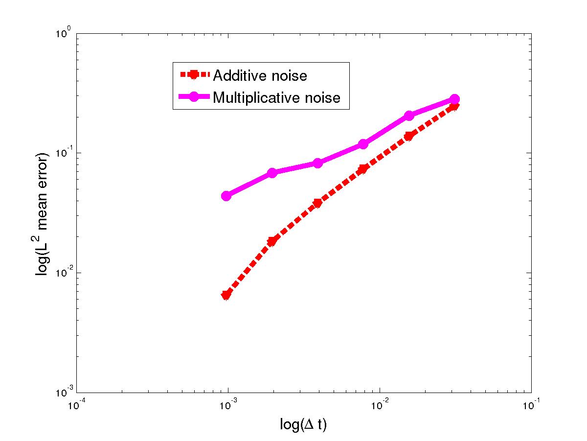
Figure 1: (a) Convergence in the root mean square $L^{2}$ norm at $T=1$ as a function of $\Delta t$. We show convergence for noise where $\beta=2$, and $\delta=10^{-3}$ in relation (105). We have used here 30 realizations. The order of convergence is $0.55$ for multiplicative noise and $0.95$ for additive noise. Graph (b) is the permeability field and graph (c) is the streamline of the velocity field $\mathbf{q}$. The mean of the solution is given in (d).

References

- [1] C. M. Elliot, S. Larsson, Error estimates with smooth and nonsmooth data for a finite element method for the Cahn-Hilliard equation, Math. Comput. 58 (1992) 603-630.
- [2] H. Fujita, A. Mizutani, On the finite element method for parabolic equation, I; approximation of holomorphic semi-groups, J. Math. Soc. Japan. 28(4)(1976) 749-771.
- [3] F. Fujita, T. Suzuki, Evolution problems (Part 1). Handbook of Numerical Analysis (P. G. Ciarlet and J.L. Lions eds), vol. 2. Amsterdam, The Netherlands: North-Holland, 1991, pp. 789-928.
- [4] S. Geiger, G. Lord, A. Tambue, Exponential time integrators for stochastic partial differential equations in 3D reservoir simulation, Computational Geosciences 16(2)(2012) 323-334.
- [5] D. Henry, Geometric Theory of semilinear parabolic Equations, Lecture notes in Mathematics, vol. 840. Berlin : Springer, 1981.
- [6] A. Jentzen, P. E. Kloeden, Overcoming the order barrier in the numerical approximation of stochastic partial differential equations with additive space–time noise, Proc. R. Soc. Lond. Ser. A Math. Phys. Eng. Sci. 465(2102) (2009) 649-667.
- [7] A. Jentzen, P. E. Kloeden, G. Winkel, Efficient simulation of nonlinear parabolic SPDEs with additive noise, Ann. Appl. Probab. 21(3)(2011) 908-950.
- [8] A. Jentzen, M. Röckner, Regularity analysis for stochastic partial differential equations with nonlinear multiplicative trace class noise, J. Diff. Equat. 252(1)(2012) 114-136.
- [9] M. Kovács, S. Larsson, F Lindgren, Strong convergence of the finite element method with truncated noise for semilinear parabolic stochastic equations with additive noise, Numer. Algor. 53(2010) 309-220.
- [10] R. Kruse, Consistency and stability of a Milstein-Galerkin finite element scheme for semilinear SPDE, Stoch. PDE: Anal. Comp. 2(2014) 471-516.
- [11] R. Kruse, Optimal error estimates of Galerkin finite element methods for stochastic partial differential equations with multiplicative noise, IMA J. Numer. Anal. 34(1)(2014) 217-251.
- [12] R. Kruse, S. Larsson, Optimal regularity for semilinear stochastic partial differential equations with multiplicative noise, Electron. J. Probab. 17(65)(2012) 1-19.
- [13] L. Lang, Adaptive Multilevel Solution of Nonlinear Parabolic PDE Systems. Theory, Algorithm, and Applications, Lecture Notes in Computational Sciences and Engineering, Vol. 16, 2000, Springer Verlag.
- [14] S. Larsson, Nonsmooth data error estimates with applications to the study of the long-time behavior of finite element solutions of semilinear parabolic problems Preprint 1992-36, Department of Mathematics, Chalmers University of Technology, 1992.
- [15] G. L. Lord, A. Tambue, Stochastic exponential integrators for the finite element discretization of SPDEs for multiplicative & additive noise, IMA J. Numer. Anal. 2(2013) 515-543.
- [16] G. L. Lord, A. Tambue, A modified semi-implicit Euler-Maruyama scheme for finite element discretization of SPDEs with additive noise, Appl. Math. Comput. 332(2018) 105-122.
- [17] J. D. Mukam, A. Tambue, Strong convergence analysis of the stochastic exponential Rosenbrock scheme for the finite element discretization of semilinear SPDEs driven by multiplicative and additive noise, J. Sci. Comput. 74(2018) 937-978.
- [18] D. Prato, G. J. Zabczyk, Stochastic equations in infinite dimensions, vol 152, 2014, Cambridge, United Kingdom: Cambrige University Press.
- [19] J. Printems, On the discretization in time of parabolic stochastic partial differential equations, Math. modelling and numer. Anal. 35(6)(2001) 1055-1078.
- [20] C. Prévôt, M. Röckner, A Concise Course on Stochastic Partial Differential Equations, Lecture Notes in Mathematics, vol. 1905, 2007, Springer, Berlin.
- [21] T. Shardlow, Numerical simulation of stochastic PDEs for excitable media, J. Comput. Appl. Math. 175(2)(2005) 429-446.
- [22] A. Tambue, Efficient Numerical Schemes for Porous Media Flow, PhD Thesis, Department of Mathematics, Heriot-Watt University, 2010.
- [23] A. Tambue, G. J. Lord, S. Geiger, An exponential integrator for advection-dominated reactive transport in heterogeneous porous media, J.Comput. Phys. 229(10)(2010) 3957-3969.
- [24] A. Tambue, An exponential integrator for finite volume discretization of a reaction-advection-diffusion equation, Comput. Math. Appl. 71(9)(2016) 1875-1897.
- [25] A. Tambue, J. M. T. Ngnotchouye, Weak convergence for a stochastic exponential integrator and finite element discretization of stochastic partial differential equation with multiplicative & additive noise, Appl. Num. Math. 108(2016) 57-86.
- [26] V. Thomée, Galerkin Finite Element Methods for Parabolic Problems, Springer-Verlag, Berlin, 1997.
- [27] X. Wang, Q. Ruisheng, A note on an accelerated exponential Euler method for parabolic SPDEs with additive noise, Appl. Math. Lett. 46(2015) 31-37.
- [28] X. Wang, Strong convergence rates of the linear implicit Euler method for the finite element discretization of SPDEs with additive noise, IMA J. Numer. Anal. 37(2017) 965-985.
- [29] Y. Yan, Galerkin finite element methods for stochastic parabolic partial differential equations, SIAM J. Num. Anal. 43(4)(2005) 1363-1384.
- [30] Y. Yan, Semidiscrete Galerkin approximation for a linear stochastic parabolic partial differential equation driven by an additive noise, BIT Numer. Math. 44(4)(2004) 829-847.