Synthetic space with arbitrary dimensions in a few rings undergoing dynamic modulation
Abstract
We show that a single ring resonator undergoing dynamic modulation can be used to create a synthetic space with an arbitrary dimension. In such a system the phases of the modulation can be used to create a photonic gauge potential in high dimensions. As an illustration of the implication of this concept, we show that the Haldane model, which exhibits non-trivial topology in two dimensions, can be implemented in the synthetic space using three rings. Our results point to a route towards exploring higher-dimensional topological physics in low-dimensional physical structures. The dynamics of photons in such synthetic spaces also provides a mechanism to control the spectrum of light.
I Introduction
It is well known that the property of a physical system depends critically on its dimension. Moreover, it has been recognized that for a lattice system, its dimension can be controlled by designing the coupling constants, i.e. the connectivity, between different sites. This has led to the development of the concept of synthetic dimension, where one explores the physics in higher dimensions using lower-dimensional physical structures tsomokos10 ; boada12 ; jukic13 ; boada15 ; suszalski16 ; taddia17 ; celi14 ; luo14 ; qi08 ; kraus13 ; lian16 ; lian17 .
As one significant recent development, it has been recognized that ring resonators provide a natural platform to explore various synthetic dimension concepts yuanOL ; yuanOptica ; ozawa16 ; qianweyl . A ring resonator supports multiple resonant modes at different frequencies. By modulating the ring dynamically, there modes can couple with one another, forming a lattice system along the frequency axis. With a particular choice of the modulation format, a ring resonator, which can be thought of conceptually as a zero-dimensional object, is described by a one-dimensional tight binding model. Consequently, one can use a -dimensional array of dynamically modulated rings to study the physics in dimension.
In this paper, we take a step further in the development of the concept of synthetic dimension using ring resonators. In a dynamically modulated ring resonator, the coupling between different modes is controlled by the modulation format yuanOptica . We show that a choice of modulation format that is different from Ref. yuanOL ; yuanOptica ; ozawa16 ; qianweyl can enable us to use a single ring to explore physics at arbitrary dimensions. And moreover, the phase degrees of freedom in the modulation naturally lead to a photonic gauge potential and associated non-trivial topology in such higher dimensional synthetic dimension yuanOL . As an example, we show that one can implement the Haldane model haldane88 , which is an important model with non-trivial topology in two-dimensions, using only three dynamically modulated resonators. Our work points to a route of exploring the very rich fundamental physics of higher dimensional system in practical physical structures. The use of the frequency axis in this implementation also leads to enhanced capability for manipulating the spectrum of light.
The paper is organized as follows: In Sec. II, we show that with a properly chosen modulation format, a single ring undergoing dynamic modulation can be mapped into a Hamiltonian that describes a lattice in arbitrary dimensions. In Sec. III, building upon the concept developed in Sec. II, we show that we can realize the Haldane model using only three ring resonators undergoing dynamic modulation. In Sec. IV, we provide a detailed simulations of the proposal in Sec. III, and highlight the experimental signature associated with this proposal. We conclude our paper in Sec. V.
II Single ring resonator supporting a synthetic two-dimensional space
We start with a single ring resonator consisting of a single-mode waveguide. Such a ring resonator supports multiple resonant modes. For the -th resonant mode, its wavevector along the waveguide needs to satisfy:
| (1) |
where is the circumference for the ring. Assuming zero group velocity dispersion in the waveguide, the resonant frequency is
| (2) |
where is the free-spectral-range of the ring. Suppose we place in the ring a phase modulator, which has a time-dependent transmission coefficient
| (3) |
where we choose the modulation frequency to be equal to and the modulation strength . is the modulation phase. In the presence of an incident wave , the transmitted wave has the form , which to the lowest order of can be approximated as . Therefore, this system can be described by the Hamiltonian
| (4) |
where is the annihilation (creation) operator for the -th mode. With , Eq. (4) becomes
| (5) |
under the rotating wave approximation. The ring resonator under modulation in the form of Eq. (3) is therefore described by the simple tight-binding model with nearest-neighbor coupling along the frequency dimension yuanOL ; yuanOptica (Figure 1(b)). As have been noted in Refs. yuanOL ; yuanOptica ; ozawa16 , the modulation phase is a gauge potential for photon. For the discussion in this section we will set to zero for simplicity.
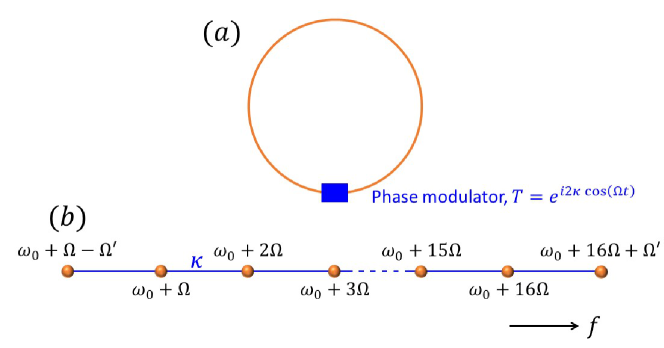
When the group velocity dispersion is not zero, the modes in the ring are no longer equally spaced and hence the modulation no longer induces on-resonance coupling. The group velocity dispersion thus results in a natural “boundary” in the frequency space yuanOL . As an illustration, in Figure 1(b), by choosing , we form a finite one-dimensional lattice with 16 resonant modes.
We now show that a more complex lattice geometry in the frequency space can be achieved by choosing other modulation formats. As an illustration, consider instead a phase modulator with the following transmission coefficient:
| (6) |
where is an integer. The additional modulation term with a modulation frequency provides a long-range coupling along the frequency axis between the -th and -th modes with the strength (see Figure 2(b)). Thus the system is now described by the Hamiltonian
| (7) |
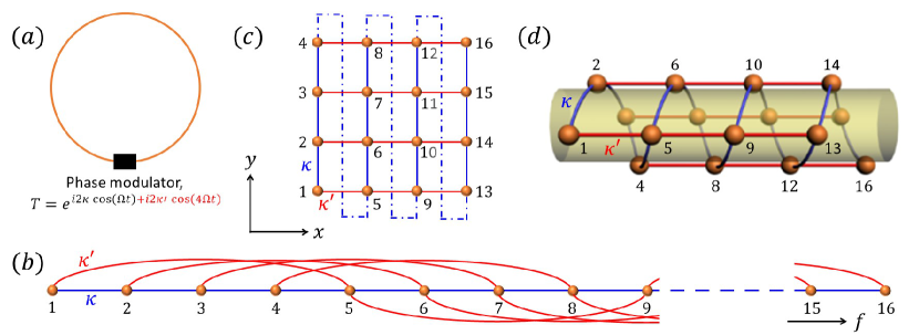
The Hamiltonian in Eq. (7) in fact represents a two-dimensional system with a twisted boundary condition. To illustrate this in details, we provide an alternative graphic representation of this Hamiltonian in Figure 2(c), for the case of , in the ring with the underlying modal structure shown in Figure 1(b) which has a boundary along the frequency axis. In this representation, the long-range coupling as described by the second term in Eq. (7), is represented by bonds along the -direction. Most of the short-range coupling as described by the first term in Eq. (7) is represented by bonds along the -direction, with the exception of the coupling between the and modes, which are represented by a “twisted” coupling between the lower and upper edge of the lattices. This “twisted” coupling can also be represented by Figure 2(d) where we see that a ring modulated with two commensurate modulation frequency can be represented by a two-dimensional lattice arranged on the surface of cylinder with a twisted periodic boundary condition. Such a geometry has a screw symmetry along the axis of the cylinder.
As illustrated above, a single ring resonator under the dynamic modulation with two modulation frequencies corresponds to a two-dimensional synthetic space. One can synthesize a higher-dimensional lattice by adding additional modulation frequencies.
III Realization of the Haldane model in the two-dimensional synthetic space with ring resonators
In the previous section, we have shown that by choosing a modulation format having two commensurate modulation frequencies, one can use a single ring resonator to achieve a synthetic two-dimensional lattice. In previous works yuanOL ; yuanOptica ; ozawa16 ; qianweyl , it was also noted that the phase of the modulation corresponds to a gauge potential in the synthetic space. In this section, as the main illustration of the paper, we show that one can combine these two ideas to realize the Haldane model using only three resonators.
The Haldane model is one of the most important models that exhibits non-trivial topological effects haldane88 . There have been several pervious works implementing the Haldane model in photonics jotzu14 ; xiao15 ; minkov16 , all of which relies upon complex lattice structures. To show that the physics of the Haldane model can be implemented in synthetic space, here we seek to implement a Hamiltonian on the honeycomb lattice:
| (8) |
where , , , and is the lattice constant. A single unit cell for this Hamiltonian is shown in Figure 3(a). The subscripts and denote the and sites of the honeycomb lattice, respectively. The terms in the first parenthesis in Eq. (8) describes nearest-neighbor coupling on a honeycomb lattice with a coupling strength . The terms in the second parenthesis in Eq. (8) describe coupling between two next-nearest-neighbor sites along the -direction, with a coupling strength and a phase .
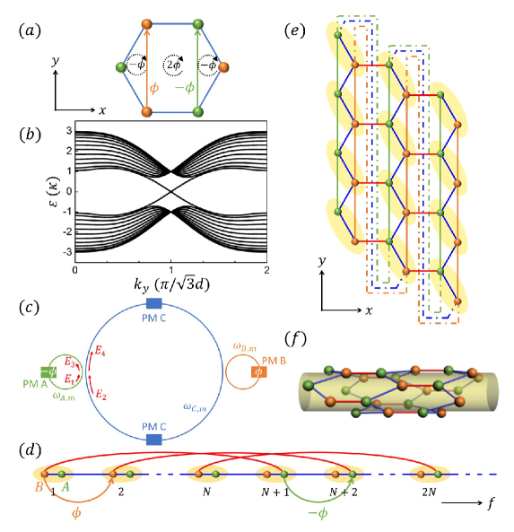
This model is a slight variant of the original model in Ref. haldane88 . The key feature of the Haldane model, which is the presence of a local magnetic field that averages to zero in each unit cell, is preserved in this Hamiltonian. As a result, the two models have very similar topologically non-trivial band structures. To illustrate the topological properties of Eq. (8), we consider a stripe that is infinite along the axis (which makes a good quantum number) and has unit cells along the axis. We set and . In the bandstructure plotted in Figure 3(b), one can see that there is a topologically nontrivial gap between the upper (and lower) bulk bands, which has Chern number +1 and -1, respectively, as evidenced by a pair of topologically-protected one-way edge states inside the gap. Such a band structure is very similar to that of the original Haldane model in Ref. haldane88 . Therefore, for the rest of the paper, we refer to the Hamiltonian of Eq. (8) as the Haldane model.
To implement the Hamiltonian in Eq. (8), we consider the geometry as shown in Figure 3(c). The geometry consists of two rings having the same circumference , labelled as and respectively. Each ring has a phase modulator inside it. The two rings also couple with each other through an auxiliary ring which has two phase modulators in it. Ring has modes with resonant frequencies . These modes corresponds to the sites in the Haldane model. Ring has modes with resonant frequencies , corresponding to the sites. Such a mode structure can be achieved, for example, by choosing an appropriate waveguide design for the ring , such that its dispersion relation is a constant shift in wavevector space with respect to that of the waveguide forming ring , i.e. . Each pair of the -th resonant mode in two rings comprises a unit cell (labelled as a pair of and sites) along the one-dimensional frequency axis in Figure 3(d).
The modulator in ring has a transmission coefficient
| (9) |
which couples two nearest-neighbor resonant modes of type . In-between two rings, we place an auxiliary ring that couples rings A and B together, as shown in Figure 3(c). The circumference of the auxiliary ring is set to be , which gives the resonance condition . The dispersion relation for the waveguide forming the ring is chosen as . Hence the resonant frequency for the ring is . Therefore, the modes in both rings and are not resonant with the modes in ring . Ring is coupled with ring with the coupling matrix
| (10) |
where is the coupling strength and () is the electric field amplitudes in both rings labelled in Figure 3(c). Ring is also coupled with ring with the same coupling matrix. On each arm of ring , we place a modulator with a time-dependent transmission coefficient:
| (11) |
Each modulator is localized at a distance away from the couplers between the rings. Referring to the one-dimensional lattice in Figure 3(d), the modulation with frequency provides the intra-cell coupling between modes inside each unit cell, the modulation with frequency provides the inter-cell coupling between and types of modes in neighbor cells, and the modulation with frequency provides a long-range coupling between the site in the -th unit cell and the site in the -th unit cell. This system can therefore be described by the Hamiltonian
| (12) |
where in the tight-binding limit.
Following the same procedure in Sec. II, one can alternatively represent the Hamiltonian (12) on a two-dimensional lattice. Mathematically, by relabelling the mode indices with respect to the honeycomb lattice, we can rewrite Eq. (12) as:
| (13) |
A specific example corresponding to 12 modes per ring, and with in Eq. (11), is shown in Figure 3(e). This Hamiltonian therefore represents a finite strip of a system described by the Haldane Hamiltonian, placed on the surface of a cylinder with a twisted boundary condition (Figure 3(f)). The system has two edges at the end of the cylinder. Therefore, we expect that one-way edge modes can exist on these edges.
IV Realistic realization in ring resonators under dynamic modulations
In the previous section we have provided a discussion for the construction of a Haldane model in synthetic space. In this section, we provide a detailed discussion of a possible experimental implementation. In particular, in the previous section we have described the effect of modulators in a simple tight-binding model, which is valid only when the modulation strength is sufficient small. In this section, we provide a more realistic description of the field propagation inside the ring under dynamic modulation. We also provide experimental signatures of one-way edge states in the synthetic space. We show that such one-way edge states can be probed by coupling input/output waveguides to the system, and by analyzing the resulting output spectrum.
To simulate the evolution of the resonant modes in both the rings and , we can expand the electric field inside the ring as hausbook
| (14) |
where the propagation direction inside the ring is given by , denotes the direction perpendicular to , is the modal profile for the ring , and gives the modal amplitude associated with the -th resonant mode. With this expansion, the Maxwell’s equations can then be converted into a set of dynamic equations for the modal amplitudes . The effect of the modulators is taken into account as a discontinuity condition for at the location of modulators in the ring. The coupling between the rings are implemented using the coupling matrix (10) at the location of the waveguide couplers. Rings and couple to external waveguides and respectively with the coupling strength with the same form of coupling matrix in Eq. (10). This procedure is described in details in Refs. yuanOL ; yuanOptica and we briefly summarize it in the Appendix.
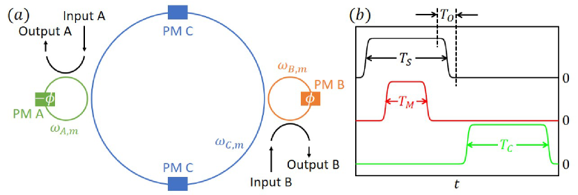
In the simulation, we assume that both rings and support 66 resonant modes (). The group velocity dispersion beyond this range provides the “boundary” along the frequency axis yuanOL . In Eq. (11), which describes the modulators inside the ring , we choose . Therefore, our design gives a two-dimensional lattice in the synthetic space. The parameters for the system in Figure 4(a) are set as , , , and . The source is injected into the system and the signal is detected through the external waveguides.
In the proposed set of experiments, we turn on the source first. After the source is turned on, we turn on the modulation over a duration of , and then turn the modulation off. Afterwards we turn off the source. The duration of the source is . After the source is turned off, we collect the output signal over a duration of in both waveguides and . We then Fourier transform the collected signal to obtain the output spectrum. We smooth all the process of turning on and off over a period of . A schematic showing this sequence of events is shown in Figure 4(b). In the following simulations, we choose and . We choose , respectively, where . And we set for each . We excite the system by an input source at the single frequency through the waveguide . We collect the output at the external waveguides and . The output spectra are then calculated by Fourier transform . The output spectra typically consist of peaks at the frequencies and for the two output waveguides, respectively.
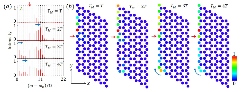
The simulation results are shown in Figure 5. As we increase , the output spectra show the signature of one-way frequency transport in the synthetic space. At , only frequency components higher than the input frequency at the 6th resonant mode are generated. At , the 11th resonant mode is significantly excited. At , the first resonant mode is excited. The spectrum then again shifts to the higher frequency direction at . This process can be also represented on the synthetic lattice as shown in Figure 5(b), where we plot the different frequency components of the and output waveguides on a honeycomb lattice as described in Section III. In this synthetic lattice, at , the light propagates along the left edge unidirectionally upward. At , it reaches the upper end of the lower edge. Due to the twisted connections between the upper and lower boundaries, once the light reaches to the left-upper corner, it transports back to the lower edge, as seen at . After that, it again travels upward, as seen in . This trajectory corresponds to one-way transport of light along the left boundary in a finite structure with a twisted boundary condition (Figure 3(f)), and represent the signature that a Haldane model can be realized in synthetic dimensional using three resonators.
To accomplish the proposed experiment above, one can use either silicon or lithium niobate ring resonators with radius of approximately with a free-spectral-range GHz. For modulation, the value of and corresponds to the efficiency for conversion to other frequencies after an incident wave with a certain frequency passes through the modulator. Our choice of and above corresponds to a conversion efficiency of and , which is reasonable for electro-optic modulators tzuangnp14 ; tzuang14 ; wang17 ; reed14 . To observe the signal with the modulation in a time scale at the order of in Figure 5 requires a loss in energy per round trip. This corresponds to a ring resonator of a quality factor up to , which is challenging but possibly achievable under the current photonic technology ilchenko04 ; savchenkov08 ; wang15 . Following this proposal, the entire structure fits into a mm2 photonic chip.
V Conclusion
In summary, we have proposed that one can achieve arbitrary dimensions in a single dynamically modulated ring resonator by choosing a particular modulation format. In addition, we find that one can construct the Haldane model in a synthetic frequency space with three dynamically modulated rings. Our study suggests that a “zero-dimensional” geometric structure can exhibit topological physics in two or even higher dimensions. The dynamic of light in this synthetic space may also provide new capabilities for the control of the spectrum of light.
Acknowledgements.
This work is supported by U.S. Air Force Office of Scientific Research Grants No. FA9550-12-1-0488, and FA9550-17-1-0002, as well as the U. S. National Science Foundation Grant No. CBET-1641069.References
- (1) D. I. Tsomokos, S. Ashhab, and F. Nori, Phys. Rev. A 82, 052311 (2010).
- (2) O. Boada, A. Celi, J. I. Latorre, and M. Lewenstein, Phys. Rev. Lett. 108, 133001 (2012).
- (3) D. Jukić and H. Buljan, Phys. Rev. A 87, 013814 (2013).
- (4) O. Boada, A. Celi, J. Rodríguez-Laguna, J. I. Latorre, and M. Lewenstein, New J. Phys. 17, 045007 (2015).
- (5) D. Suszalski and J. Zakrzewski, Phys. Rev. A 94, 033602 (2016).
- (6) L. Taddia, E. Cornfeld, D. Rossini, L. Mazza, E. Sela, and R. Fazio, Phys. Rev. Lett. 118, 230402 (2017).
- (7) A. Celi, P. Massignan, J. Ruseckas, N. Goldman, I. B. Spielman, G. Juzeliūnas, and M. Lewenstein, Phys. Rev. Lett. 112, 043001 (2014).
- (8) X.-W. Luo, X. Zhou, C.-F. Li, J.-S. Xu, G.-C. Guo, and Z.-W. Zhou, Nat. Commun. 6, 7704 (2014).
- (9) X. Qi, T. L. Hughes, and S. Zhang, Phys. Rev. B 78, 195424 (2008).
- (10) Y. E. Kraus, Z. Ringel, and O. Zilberberg, Phys. Rev. Lett. 111, 226401 (2013).
- (11) B. Lian and S. Zhang, Phys. Rev. B 94, 041105R (2016).
- (12) B. Lian and S. Zhang, Phys. Rev. B 95, 235106 (2017).
- (13) L. Yuan, Y. Shi, and S. Fan, Opt. Lett. 41, 741 (2016).
- (14) L. Yuan and S. Fan, Optica 3, 1014 (2016).
- (15) T. Ozawa, H. M. Price, N. Goldman, O. Zilberberg, and I. Carusotto, Phys. Rev. A 93, 043827 (2016).
- (16) Q. Lin, M. Xiao, L. Yuan, and S. Fan, Nat. Commun. 7, 13731 (2016).
- (17) F. D. M. Haldane, Phys. Rev. Lett. 61, 2015 (1988).
- (18) G. Jotzu, M. Messer, R. Desbuquois, M. Lebrat, T. Uehlinger, D. Greif, and T. Esslinger, Nature 515, 237 (2014).
- (19) M. Xiao, W.-J. Chen, W.-Y. He, and C. T. Chan, Nat. Phys. 11, 920 (2015).
- (20) M. Minkov and V. Savona, Optica 3, 200 (2016).
- (21) H. A. Haus, Waves and fields in optoelectronics (Prentice-Hall, Inc., Englewood Cliffs, NJ, 1984).
- (22) L. D. Tzuang, K. Fang, P. Nussenzveig, S. Fan, and M. Lipson, Nat. Photonics 8, 701 (2014).
- (23) L. D. Tzuang, M. Soltani, Y. H. D. Lee, and M. Lipson, Opt. Lett. 39, 1799 (2014).
- (24) C. Wang, M. Zhang, B. Stern, M. Lipson, M. Loncar, arXiv:1701.06470.
- (25) G. T. Reed, G. Z. Mashanovich, F. Y. Gardes, M. Nedeljkovic, Y. Hu, D. J. Thomson, K. Li, P. R. Wilson, S. Chen, and S. S. Hsu, Nanophotonics 3, 229 (2014).
- (26) V. S. Ilchenko, A. A. Savchenkov, A. B. Matsko, and L. Maleki, Phys. Rev. Lett. 92, 043903 (2004).
- (27) A. A. Savchenkov, A. B. Matsko, V. S. Ilchenko, I. Solomatine, D. Seidel, and L. Maleki, Phys. Rev. Lett. 101, 093902 (2008).
- (28) J. Wang, F. Bo, S. Wan, W. Li, F. Gao, J. Li, G. Zhang, and J. Xu, Opt. Express 23, 23072 (2015).
Appendix — simulation method based on the modal expansion of the electric field
We study the evolution of the resonant modes in both the rings and . The modal amplitude at the -th resonant mode defined in Eq. (14) obeys the equation hausbook2 ; yuanOL2 ; yuanOptica2
| (A-1) |
under the slowly-varying-envelope approximation and the boundary condition . Here is the group index and is assumed to be constant in the regime with the zero group velocity dispersion.
The resonant modes in and are off resonance from the modes in , since light is injected into ring only through rings and , we therefore expand the field inside ring with only the field components that are resonant in the ring :
| (A-2) |
The associated mode amplitude satisfies
| (A-3) |
under the slowly-varying-envelope approximation and .
The modulators in the rings have transmission coefficients described by Eqs. (9) and (11). At the location of these modulators, the modal amplitudes satisfy Saleh :
| (A-4) |
| (A-5) |
| (A-6) |
where the rotating wave approximation is used. is the -th order Bessel function and . denote the position of the modulators in each ring in Figure 4(a). In Eq. (A-4), which describes the modulators in rings and , we expand the transmission coefficient as described by Eq. (9) to all orders of its Fourier coefficients. On the other hand, in Eqs. (A-5) and (A-6), which describes the modulators in ring , we expand the transmission coefficient of Eq. (11) and keep only the lowest frequency components to the 1st order. We also keep only the contributions from the field components that are resonant in the ring . This expansion is reasonable since ring is non-resonant.
The coupling between rings or and ring is described by:
| (A-7) |
| (A-8) |
where is the coupling strength between rings. The s denote the positions of the coupler in the rings as specfied by the subscript. The coupling between the rings () and the external waveguides () is given by
| (A-9) |
| (A-10) |
where is the input/output amplitude of the field component at the frequency mode in the external waveguides () and is the coupling strength. The s denote the position of the coupler between the external waveguides and the rings.
References
- (1) H. A. Haus, Waves and fields in optoelectronics (Prentice-Hall, Inc., Englewood Cliffs, NJ, 1984).
- (2) L. Yuan, Y. Shi, and S. Fan, Opt. Lett. 41, 741 (2016).
- (3) L. Yuan and S. Fan, Optica 3, 1014 (2016).
- (4) B. E. A. Saleh, M. C. Teich, Fundamentals of Photonics, 2nd ed. (Wiley-Interscience, Hoboken, N.J. 2007).