Heat transfer in a one-dimensional harmonic crystal in a viscous environment subjected to an external heat supply

Abstract

We consider unsteady heat transfer in a one-dimensional harmonic crystal surrounded by a viscous environment and subjected to an external heat supply. The basic equations for the crystal particles are stated in the form of a system of stochastic differential equations. We perform a continualization procedure and derive an infinite set of linear partial differential equations for covariance variables. An exact analytic solution describing unsteady ballistic heat transfer in the crystal is obtained. It is shown that the stationary spatial profile of the kinetic temperature caused by a point source of heat supply of constant intensity is described by the Macdonald function of zero order. A comparison with the results obtained in the framework of the classical heat equation is presented. We expect that the results obtained in the paper can be verified by experiments with laser excitation of low-dimensional nanostructures.

1 Introduction

An understanding of heat transfer at the microlevel is essential to obtain a link between the microscopic and the macroscopic descriptions of solids. As far as the macroscopic level is concerned, Fourier’s law of heat conduction is widely and successfully used to describe heat transfer processes. However, it is well known that for one-dimensional crystals substantial deviations from Fourier’s law are observed rieder1967properties ; bonetto2000mathematical ; lepri2003thermal ; 0295-5075-43-3-271 ; dhar2008heat . Extensive investigations over the last decades were devoted to resolving these anomalies, many of the recent developments in this area are reviewed in book Lepri2016thermal . One of the possible solutions is to use special laws of particle interactions casati1984one ; aoki2000bulk ; gendelman2014normal ; savin2014thermal ; gendelman2016heat , in particular, systems on a nonlinear elastic support with no momentum conservation aoki2000bulk , or systems possessing the possibility of bond break gendelman2014normal ; savin2014thermal ; gendelman2016heat . Such systems under certain conditions demonstrate normal heat conductivity even in one dimension. As it is shown in spohn2016fluctuating , one-dimensional case is still very specific, therefore, another way to avoid anomalies is to use sufficiently complex structures and increase the system dimensionality bonetto2004fourier ; le2008molecular . However, recent experimental observations demonstrate that Fourier’s law is indeed violated in low-dimensional nanostructures chang2008breakdown ; xu2014length ; hsiao2015micron ; cahill2003nanoscale ; liu2012anomalous ; lepri2016thermal8 , where the ballistic heat transfer is realized. This fact is in agreement with the phonon theory peierls1955quantum ; ziman1960electrons , which relates the heat conductivity with the phonon mean free path. At the macroscale, the phonon mean free path is a small quantity in comparison with the characteristic size of the system, but this is not true for microscale and nanoscale systems hsiao2013observation . This motivates the interest in the simplest lattice models, in particular, in harmonic one-dimensional crystals (chains), where these anomalies are most prominent kannan2012nonequilibrium ; dhar2015heat . Problems of this type were previously addressed mainly in the context of steady-state heat conduction bonetto2000mathematical ; lepri2003thermal ; 0295-5075-43-3-271 ; dhar2008heat ; rieder1967properties ; allen1969energy ; nakazawa1970lattice ; lee2005heat ; kundu2010heat ; lepri2016thermal2 ; bernardin2012harmonic ; freitas2014analytic ; freitas2014erratum ; hoover2013hamiltonian ; lukkarinen2016harmonic , unsteady conduction regimes came into the focus in le2008molecular ; gendelman2012nonstationary ; tsai1976molecular ; ladd1986lattice ; volz1996transient ; daly2002molecular ; gendelman2010nonstationary ; babenkov2016energy ; krivtsov2015heat ; krivtsov2014energy .

Simple lattice models can be used for the analytical investigation of the thermomechanical processes in solids at the microscale hoover2015simulation ; daly2002molecular ; krivtsov2003nonlinear ; berinskii2016elastic ; kuzkin2016lattice , and, in particular, in the carbon nanostructures berinskii2015linear ; berinskii2016hyperboloid . One-dimensional systems due to their simplicity can be used to obtain analytical solutions in a closed form without loss of generality krivtsov2003nonlinear ; dhar2008heat ; Gavrilov-Shishkina-MMS ; gendelman2010nonstationary , or to get the asymptotic description of non-stationary processes in media with complex structure Gavrilov_SN–ZAMM87N2-2007-p117_127 ; Gavrilov_SN-Shishkina_EV–CMT22-2010-p299_316 ; Gavrilov-Shishkina-ZAMM ; Gavrilov-Shishkina-MMS ; shishkina2017stiff ; Gavrilov-JSV-2012 . In previous studies krivtsov2014energy ; krivtsov2015heat ; krivtsov2017heat , a new approach was suggested which allows one to solve analytically non-stationary thermal problems for a one-dimensional harmonic crystal — an infinite ordered chain of identical material particles, interacting via linear (harmonic) forces. In particular, a heat transfer equation was obtained that differ from the extended heat transfer equations suggested earlier chandrasekharalah1986thermoelasticity ; tzou2014macro ; cattaneo1958forme ; vernotte1958paradoxes ; however, it is in an excellent agreement with molecular dynamics simulations and previous analytical estimates gendelman2012nonstationary . Later this approach was generalized to a number of systems, namely, to a one-dimensional crystal on an elastic substrate babenkov2016energy , and to two and three-dimensional harmonic crystals kuzkin2017analytical ; Kuzkin-Krivtsov-accepted . In the most of above mentioned papers krivtsov2014energy ; krivtsov2015heat ; babenkov2016energy ; kuzkin2017analytical ; Kuzkin-Krivtsov-accepted only isolated systems were considered. The motivation for this paper is to consider a system that can exchange energy with its surroundings. Therefore, now we assume that the crystal is surrounded by a viscous environment (a gas or a liquid) which causes an additional dissipative term in the equations of stochastic dynamics for the particles. Additionally, we take into account sources of heat supply. This is a more realistic model, and thus we expect that the theoretical results obtained in the paper can be verified by experiments with laser excitation of low-dimensional nanostructures lepri2016thermal8 ; liu2012anomalous ; cahill2003nanoscale ; indeitsev2017two .

The paper is organized as follows. In Section 2, we consider the formulation of the problem. In Section 2.1, some general notation is introduced. In Section 2.2, we state the basic equations for the crystal particles in the form of a system of stochastic differential equations. In Section 2.3, we introduce and deal with infinite set of covariance variables. These are the mutual covariances of the particle velocities and the displacements for all pairs of particles. We use the Itô lemma to derive (see Appendix A) an infinite deterministic system of ordinary differential equations which follows from the equations of stochastic dynamics. This system can be transformed into an infinite system of differential-difference equations involving only the covariances for the particle velocities. In Section 3, we introduce a continuous spatial variable and write the finite difference operators involved in the equation for covariances as compositions of finite difference operators and operators of differentiation. To do this, we use some identities of the calculus of finite differences (see Appendix B). In Section 4, we perform an asymptotic uncoupling of the equation for covariances. Provided that the introduced continuous spatial variable can characterize the behavior of the crystal, one can distinguish between slow motions, which are related to the heat propagation, and vanishing fast motions krivtsov2014energy ; babenkov2016energy , which are not considered in the paper. Slow motions can be described by a coupled infinite system of second-order hyperbolic partial differential equations for quantities which we call the non-local temperatures. The zero-order non-local temperature, which is proportional to the statistical dispersion of the particle velocities, is the classical kinetic temperature. In Section 5, we obtain an expression for the fundamental solution for the kinetic temperature and solve the non-stationary problem of the heat propagation from a suddenly applied point source of constant intensity. In contrast to the case of a crystal without viscous environment (Section 5.1), in the case of a crystal surrounded by a viscous environment (Section 5.2) there exists a steady-state solution describing the kinetic temperature distribution caused by a constant point source. In Section 6, we present the results of the numerical solution of the initial value problem for the system of stochastic differential equations and compare them with the obtained analytical solution. In Section 7, we compare our results with the classical results obtained in the framework of the heat equation based on Fourier’s law. In the conclusion (Section 8), we discuss the basic results of the paper.

2 Mathematical formulation

2.1 Notation

In the paper, we use the following general notation:

$t$

the time;

$H(\cdot)$

the Heaviside function;

$\delta(\cdot)$

the Dirac delta function;

$\langle\cdot\rangle$

the expected value for a random quantity;

$\delta_{pq}$

is the Kronecker delta ($\delta_{pq}=1$ if $p=q$, and $\delta_{pq}=0$ otherwise);

$\delta_{n}$

$\delta_{n}=1$ if $n=0$ and $\delta_{n}=0$ otherwise;

$J_{0}(\cdot)$

the Bessel function of the first kind of zero order andrewsspecial ;

$I_{0}(\cdot)$

the modified Bessel function of the first kind of zero order andrewsspecial ;

$K_{0}(\cdot)$

the Macdonald function (the modified Bessel function of the second kind) of zero order andrewsspecial ;

$\operatorname{erfc}(\cdot)$

the complementary error function andrewsspecial .

2.2 Stochastic crystal dynamics

Consider the following system of stochastic ordinary differential equations kloeden1999 ; stepanov2013stochastic :

$$dv_{i}=F_{i}dt+b_{i}dW_{i},\qquad du_{i}=v_{i}dt,$$ (2.1)

where

$$F_{i}={\color[rgb]{0,0,0}\omega_{0}^{2}{\mathcal{L}}}_{i}u_{i}-\eta v_{i},$$ (2.2)

$$dW_{i}=\rho_{i}\sqrt{dt},$$ (2.3)

$$\omega_{0}\stackrel{{\scriptstyle\mbox{\scriptsize def}}}{{=}}\sqrt{C/m},$$ (2.4)

Here $i$ is an arbitrary integer which describes the position of a particle in the chain; the stochastic processes $u_{i}(t)$ and $v_{i}(t)$ are the displacement and the particle velocity, respectively; $F_{i}$ is the specific force on the particle; $W_{i}$ are Wiener processes; $b_{i}(t)$ is the intensity of the random external excitation; $\eta$ is the specific viscosity for the environment; $C$ is the bond stiffness; $m$ is the mass of a particle; ${\mathcal{L}}_{i}$ is the linear finite difference operator:

$${\mathcal{L}}_{i}u_{i}=u_{i+1}-2u_{i}+u_{i-1}.$$ (2.5)

Note that the results of the paper can be generalized for more complex finite difference operators and related physical systems (e.g. a crystal on an elastic support, next neighbour interactions etc).

The normal random variables $\rho_{i}$ are such that

$$\langle{\rho_{i}}\rangle=0,\qquad\langle{\rho_{i}\rho_{j}}\rangle=\delta_{ij},$$ (2.6)

and they are assumed to be independent of $u_{i}$ and $v_{i}$. The initial conditions are zero: for all $i$,

$$u_{i}(0)=0,\qquad v_{i}(0)=0.$$ (2.7)

In the case $b_{i}\equiv b$, equations (2.1) are the Langevin equations langevin1908theorie ; lemons1997paul for a one-dimensional harmonic crystal (an ordered chain of identical interacting material particles, see Fig. 1) surrounded by a viscous environment (e.g., a gas or a liquid). Assuming that $b_{i}$ may depend on $i$, we introduce a natural generalization of the Langevin equation which allows one to describe the possibility of an external heat excitation (e.g., laser excitation). This external excitation is assumed to be localized in space (in the paper we mostly consider the case of a point heat source) and much more intensive than the stochastic influence caused by a non-zero temperature of the environment. Therefore, we neglect in (2.1) the constant stochastic term that does not depend on $i$. Note that since $b_{i}$ do not depend on $u_{j}$ and $v_{j}$ for all $i,j$, it is not necessary to distinguish between the Stratonovich and Itô formalism kloeden1999 in the case of equation (2.1).

Figure 1: A one-dimensional harmonic crystal.

2.3 The dynamics of covariances

According to (2.2), $F_{i}$ are linear functions of $u_{i},\ v_{i}$. Taking this fact into account together with (2.6) and (2.7), we see that for all $t$

$$\langle{u_{i}}\rangle=0,\qquad\langle{v_{i}}\rangle=0.$$ (2.8)

Following krivtsov2016ioffe , consider the infinite sets of covariance variables

$$\xi_{p,q}\stackrel{{\scriptstyle\mbox{\scriptsize def}}}{{=}}\langle{u_{p}u_{q}}\rangle,\qquad\nu_{p,q}\stackrel{{\scriptstyle\mbox{\scriptsize def}}}{{=}}\langle{u_{p}v_{q}}\rangle,\qquad\kappa_{p,q}\stackrel{{\scriptstyle\mbox{\scriptsize def}}}{{=}}\langle{v_{p}v_{q}}\rangle,$$ (2.9)

and the quantities

$$\beta_{p,q}\stackrel{{\scriptstyle\mbox{\scriptsize def}}}{{=}}\delta_{pq}\,b_{p}b_{q}.$$ (2.10)

In the last equation, we take into account the second equation of (2.6). Thus the variables $\xi_{p,q},\ \nu_{p,q},\ \kappa_{p,q}$ and $\beta_{p,q}$ are defined for any pair of crystal particles. For simplicity, in what follows we drop the subscripts $p$ and $q$, i.e., $\xi\stackrel{{\scriptstyle\mbox{\scriptsize def}}}{{=}}\xi_{p,q}$ etc. By definition, we also put $\xi^{\top}\stackrel{{\scriptstyle\mbox{\scriptsize def}}}{{=}}\xi_{q,p}$ etc. Now we differentiate the variables (2.9) with respect to time taking into account the equations of motion (2.1). This yields the following closed system of differential equations for the covariances (see Appendix A):

$$\begin{gathered}\partial_{t}\xi=\nu+\nu^{\top},\\ \partial_{t}\nu+\eta\nu={\color[rgb]{0,0,0}\omega_{0}^{2}{\mathcal{L}}}_{q}\xi+\kappa,\\ \partial_{t}\kappa+2\eta\kappa={\color[rgb]{0,0,0}\omega_{0}^{2}{\mathcal{L}}}_{p}\nu+{\color[rgb]{0,0,0}\omega_{0}^{2}{\mathcal{L}}}_{q}\nu^{\top}+\beta,\end{gathered}$$ (2.11)

where $\partial_{t}$ is the operator of differentiation with respect to time; ${\mathcal{L}}_{p}$ and ${\mathcal{L}}_{q}$ are the linear difference operators defined by (2.5) that act on $\xi_{p,q},\ \nu_{p,q},\ \kappa_{p,q},\ \beta_{p,q}$ with respect to the first index subscript $p$ and the second one $q$, respectively. Now we introduce the symmetric and antisymmetric difference operators

$$2{\mathcal{L}}^{\mathrm{S}}\stackrel{{\scriptstyle\mbox{\scriptsize def}}}{{=}}{\mathcal{L}}_{p}+{\mathcal{L}}_{q},\qquad 2{\mathcal{L}}^{\mathrm{A}}\stackrel{{\scriptstyle\mbox{\scriptsize def}}}{{=}}{\mathcal{L}}_{p}-{\mathcal{L}}_{q},$$ (2.12)

and the symmetric and antisymmetric parts of the variable $\nu$:

$$2\nu^{\mathrm{S}}\stackrel{{\scriptstyle\mbox{\scriptsize def}}}{{=}}\nu+\nu^{\top},\qquad 2\nu^{\mathrm{A}}\stackrel{{\scriptstyle\mbox{\scriptsize def}}}{{=}}\nu-\nu^{\top}.$$ (2.13)

Note that $\xi$ and $\kappa$ are symmetric variables. Now equations (2.11) can be rewritten as follows:

$$\partial_{t}\xi=2\nu^{\mathrm{S}},\qquad(\partial_{t}+2\eta)\kappa=2{\color[rgb]{0,0,0}\omega_{0}^{2}{\mathcal{L}}}^{\mathrm{S}}\nu^{\mathrm{S}}+2{\color[rgb]{0,0,0}\omega_{0}^{2}{\mathcal{L}}}^{\mathrm{A}}\nu^{\mathrm{A}}+\beta,$$ (2.14)

$$(\partial_{t}+\eta)\nu^{\mathrm{A}}=-{\color[rgb]{0,0,0}\omega_{0}^{2}{\mathcal{L}}}^{\mathrm{A}}\xi,\qquad(\partial_{t}+\eta)\nu^{\mathrm{S}}={\color[rgb]{0,0,0}\omega_{0}^{2}{\mathcal{L}}}^{\mathrm{S}}\xi+\kappa.$$ (2.15)

Applying the operator $\partial_{t}+\eta$ to Eqs. (2.14) and substituting expressions (2.15) yields a closed system of two equations of second order in time:

$$\partial_{t}(\partial_{t}+\eta)\xi=2({\color[rgb]{0,0,0}\omega_{0}^{2}{\mathcal{L}}}^{\mathrm{S}}\xi+\kappa),$$ (2.16)

$$(\partial_{t}+\eta)(\partial_{t}+2\eta)\kappa=2\big{(}({\color[rgb]{0,0,0}\omega_{0}^{2}{\mathcal{L}}}^{\mathrm{S}})^{2}-({\color[rgb]{0,0,0}\omega_{0}^{2}{\mathcal{L}}}^{\mathrm{A}})^{2}\big{)}\xi+2{\color[rgb]{0,0,0}\omega_{0}^{2}{\mathcal{L}}}^{\mathrm{S}}\kappa+(\partial_{t}+\eta)\beta.$$ (2.17)

We can express $\kappa$ in terms of $\xi$ using Eq. (2.16):

$$\kappa=\frac{1}{2}(\partial_{t}^{2}+\eta\partial_{t}-2{\color[rgb]{0,0,0}\omega_{0}^{2}{\mathcal{L}}}^{\mathrm{S}})\xi,$$ (2.18)

and substitute the result into Eq. (2.17). This yields

$$\frac{1}{2}\Big{(}\big{(}(\partial_{t}+\eta)(\partial_{t}+2\eta)-2{\color[rgb]{0,0,0}\omega_{0}^{2}{\mathcal{L}}}^{\mathrm{S}}\big{)}(\partial_{t}^{2}+\eta\partial_{t}-2{\color[rgb]{0,0,0}\omega_{0}^{2}{\mathcal{L}}}^{\mathrm{S}})-4\big{(}({\color[rgb]{0,0,0}\omega_{0}^{2}{\mathcal{L}}}^{\mathrm{S}})^{2}-({\color[rgb]{0,0,0}\omega_{0}^{2}{\mathcal{L}}}^{\mathrm{A}})^{2}\Big{)}\xi\\ =(\partial_{t}+\eta)\beta.$$ (2.19)

Simplifying the left-hand side of Eq. (2.19) results in an equation of fourth order in time for $\xi$:

$$\big{(}(\partial_{t}+\eta)^{2}(\partial_{t}^{2}+2\eta\partial_{t}-4{\color[rgb]{0,0,0}\omega_{0}^{2}{\mathcal{L}}}^{\mathrm{S}})+4({\color[rgb]{0,0,0}\omega_{0}^{2}{\mathcal{L}}}^{\mathrm{A}})^{2}\big{)}\xi=2(\partial_{t}+\eta)\beta.$$ (2.20)

Now we apply the operator $\frac{1}{2}(\partial_{t}^{2}+\eta\partial_{t}-2{\color[rgb]{0,0,0}\omega_{0}^{2}{\mathcal{L}}}^{\mathrm{S}})$ to Eq. (2.20). Taking into account (2.18), this yields a fourth-order equation for the covariances of the particle velocities $\kappa$:

$$\left((\partial_{t}+\eta)^{2}(\partial_{t}^{2}+2\eta\partial_{t}-4{\color[rgb]{0,0,0}\omega_{0}^{2}{\mathcal{L}}}^{\mathrm{S}})+4({\color[rgb]{0,0,0}\omega_{0}^{2}{\mathcal{L}}}^{\mathrm{A}})^{2}\right)\kappa=(\partial_{t}+\eta)(\partial_{t}^{2}+\eta\partial_{t}-2{\color[rgb]{0,0,0}\omega_{0}^{2}{\mathcal{L}}}^{\mathrm{S}})\beta.$$ (2.21)

In what follows, we deal with Eq. (2.21). According to Eqs. (2.7), (2.9), we supplement Eq. (2.21) with zero initial conditions. We state these conditions in the following form, which is conventional for distributions (or generalized functions) Vladimirov1971 :

$$\kappa\big{|}_{t<0}\equiv 0.$$ (2.22)

To take into account non-zero classical initial conditions, one needs to add the corresponding singular terms (in the form of a linear combination of $\delta(t)$ and its derivatives) to the right-hand sides of the corresponding equations Vladimirov1971 .

Let us note that equation (2.21) is a determenistic equation. What is also important is that (2.21) is a closed equation. Thus the thermal processes do not depend on any property of the cumulative distribution functions for the displacements and the particle velocities other than the covariance variables used above.

3 Continualization of the finite difference operators

In this section, we use some identities of the calculus of finite differences (see Appendix B). Following krivtsov2015heat ; krivtsov2016ioffe , we introduce the discrete spatial variable

$$k\stackrel{{\scriptstyle\mbox{\scriptsize def}}}{{=}}p+q$$ (3.1)

and the discrete correlational variable

$$n\stackrel{{\scriptstyle\mbox{\scriptsize def}}}{{=}}q-p$$ (3.2)

instead of discrete variables $p$ and $q$. We can also formally introduce the continuous spatial variable

$$x\stackrel{{\scriptstyle\mbox{\scriptsize def}}}{{=}}\frac{ak}{2},$$ (3.3)

where $a$ is the lattice constant (the distance between neighboring particles). We have

$$q=\frac{x}{a}+\frac{n}{2},\qquad p=\frac{x}{a}-\frac{n}{2}.$$ (3.4)

To perform the continualization, we assume that the lattice constant is an infinitesimal quantity and introduce a dimensionless formal small parameter $\epsilon$ in the following way:

$$a=\epsilon\hat{a},$$ (3.5)

where $\hat{a}=O(1)$. To preserve the speed of sound in the crystal $c\stackrel{{\scriptstyle\mbox{\scriptsize def}}}{{=}}a\omega_{0}$ as a quantity of order $O(1)$, we additionally assume that

$$\omega_{0}=\epsilon^{-1}\hat{\omega}_{0},$$ (3.6)

where $\hat{\omega}_{0}=O(1)$. Thus $c=\hat{a}\hat{\omega}_{0}=O(1)$. The basic assumption that allows one to perform the continualization is that any quantity $\zeta_{p,q}$ defined by (2.9) or (2.10), where $p$ and $q$ are defined by (3.4), can be calculated as a value of a smooth function $\hat{\zeta}_{n}(x)$ of the continuous spatial slowly varying coordinate

$$x=\frac{\epsilon\hat{a}k}{2}$$ (3.7)

and the discrete correlational variable $n$:

$$\hat{\zeta}_{n}(x)\stackrel{{\scriptstyle\mbox{\scriptsize def}}}{{=}}\zeta_{k+\tfrac{n}{2},k-\tfrac{n}{2}}=\zeta_{p,q}.$$ (3.8)

In accordance with (3.8), one has

$$\begin{gathered}{\mathcal{L}}_{p}\zeta_{p,q}=\hat{\zeta}_{n-1}\left(x+\tfrac{a}{2}\right)-2\hat{\zeta}_{n}(x)+\hat{\zeta}_{n+1}\left(x-\tfrac{a}{2}\right),\\ {\mathcal{L}}_{q}\zeta_{p,q}=\hat{\zeta}_{n+1}\left(x+\tfrac{a}{2}\right)-2\hat{\zeta}_{n}(x)+\hat{\zeta}_{n-1}\left(x-\tfrac{a}{2}\right).\end{gathered}$$ (3.9)

Applying the Taylor theorem to these formulas yields

$${\mathcal{L}}_{p}\zeta_{p,q}={\mathcal{L}}_{n}\hat{\zeta}_{n}+\tfrac{a}{2}\,\partial_{x}(\hat{\zeta}_{n-1}-\hat{\zeta}_{n+1})$$ (3.10)

$$\qquad\qquad\qquad+\tfrac{a^{2}}{8}\,\partial_{x}^{2}(\hat{\zeta}_{n-1}+\hat{\zeta}_{n+1})+o(\epsilon^{2}),$$

$${\mathcal{L}}_{q}\zeta_{p,q}={\mathcal{L}}_{n}\hat{\zeta}_{n}+\tfrac{a}{2}\,\partial_{x}(\hat{\zeta}_{n+1}-\hat{\zeta}_{n-1})$$

$$\qquad\qquad\qquad+\tfrac{a^{2}}{8}\,\partial_{x}^{2}(\hat{\zeta}_{n+1}+\hat{\zeta}_{n-1})+o(\epsilon^{2}).$$

An alternative way of continualization can be realized by letting the number of particles diverge, rather than invoking an increasingly small separation lepri2010nonequilibrium . Despite the algorithmic difference, these approaches lead to the same result.

Now we perform the continualization of the operators ${\mathcal{L}}^{\mathrm{S}},\ {\mathcal{L}}^{\mathrm{A}}$. Using (3.10), we obtain

$${\mathcal{L}}^{\mathrm{S}}={\mathcal{L}}_{n}+O(\epsilon^{2}),$$ (3.11)

$${\mathcal{L}}^{\mathrm{A}}=-\tfrac{a}{2}\,\mathscr{D}_{n}\partial_{x}+O(\epsilon^{2}),$$ (3.12)

where

$$\mathscr{D}_{n}f_{n}=f_{n+1}-f_{n-1}.$$ (3.13)

Now we calculate $({\mathcal{L}}^{\mathrm{A}})^{2}$ using (3.12), (B.6), (B.10). This yields

$$({\mathcal{L}}^{\mathrm{A}})^{2}=a^{2}{\cal M}+o(\epsilon^{2}),$$ (3.14)

$${\cal M}\stackrel{{\scriptstyle\mbox{\scriptsize def}}}{{=}}-\frac{1}{4}{\mathcal{L}}_{n}(-1)^{n}{\mathcal{L}}_{n}(-1)^{n}\partial_{x}^{2}.$$ (3.15)

4 Slow motions

Taking into account assumption (3.6), Eq. (2.21) can be rewritten in the following form:

$$\bigg{(}(\partial_{t}+\eta)^{2}\big{(}\epsilon^{2}(\partial_{t}^{2}+2\eta\partial_{t})-4\hat{\omega}_{0}^{2}{\mathcal{L}}^{\mathrm{S}}\big{)}+4\frac{\hat{\omega}_{0}^{4}}{\epsilon^{2}}({\mathcal{L}}^{\mathrm{A}})^{2}\bigg{)}\kappa\\ =(\partial_{t}+\eta)\big{(}\epsilon^{2}(\partial_{t}^{2}+\eta\partial_{t})-2\hat{\omega}_{0}^{2}{\mathcal{L}}^{\mathrm{S}}\big{)}\beta.$$ (4.1)

Equation (4.1) is a differential equation whose highest derivative with respect to $t$ is multiplied by a small parameter. Therefore, one can expect the existence of two types of solutions, namely, solutions slowly varying in time and fast varying in time nayfeh2008perturbation . The presence of fast and slow motions is a standard property of statistical systems. Fast motions are oscillations of temperature caused by equilibration of kinetic and potential energies. Slow motions are related with macroscopic heat propagation.

Considering slow motions, we assume that

$$\epsilon^{2}(\partial_{t}^{2}+2\eta\partial_{t})\kappa\ll\hat{\omega}_{0}^{2}{\mathcal{L}}^{\mathrm{S}}\kappa,\qquad\epsilon^{2}(\partial_{t}^{2}+\eta\partial_{t})\beta\ll\hat{\omega}_{0}^{2}{\mathcal{L}}^{\mathrm{S}}\beta.$$ (4.2)

Vanishing solutions that characterize fast motions, which do not satisfy (4.2), are not considered in this paper. In krivtsov2014energy , the properties of fast motions are investigated in the case of the system under consideration without viscous environment ($\eta=0$) and external heating ($\beta=0$). In babenkov2016energy , fast motions in a one-dimensional harmonic crystal on an elastic substrate are considered (again under the zero external action condition).

Now, taking into account (3.14), we drop the higher order terms and rewrite equation (4.1) in the form of an equation for slow motions:

$$2\big{(}(\partial_{t}+\eta)^{2}{\mathcal{L}}^{\mathrm{S}}-c^{2}{\cal M}\big{)}\kappa=(\partial_{t}+\eta){\mathcal{L}}^{\mathrm{S}}\beta.$$ (4.3)

Applying the operator $({\mathcal{L}}^{\mathrm{S}})^{-1}$ to Eq. (4.3) results in

$$\ddot{\kappa}+2\eta\dot{\kappa}+\big{(}\eta^{2}-c^{2}({\mathcal{L}}^{\mathrm{S}})^{-1}{\cal M}\big{)}\kappa=\frac{1}{2}(\dot{\beta}+\eta\beta)+C,$$ (4.4)

where ${\mathcal{L}}^{\mathrm{S}}C\equiv 0$. Here and in what follows we use more compact notaton: the overdot means $\partial_{t}$, the prime means $\partial_{x}$. Taking into account the initial conditions in the form of Eq. (2.22), one can show that $C=0$.

Now we perform the continualization of the equations. According to Eqs. (3.11), (3.14), (3.15), we have

$$({\mathcal{L}}^{\mathrm{S}})^{-1}{\cal M}=-\frac{1}{4}(-1)^{n}{\mathcal{L}}_{n}(-1)^{n}\partial_{x}^{2}+o(\epsilon^{2}).$$ (4.5)

Now we multiply (4.4) by $(-1)^{n}mk_{B}^{-1}$ (here $k_{\!B}$ is the Boltzmann constant), and rewrite Eq. (4.4) in the following form:

$$\textstyle\ddot{\theta}_{n}+2\eta\dot{\theta}_{n}+\eta^{2}\theta_{n}+\frac{c^{2}}{4}{\mathcal{L}}_{n}\theta_{n}^{\prime\prime}=(\dot{\chi}+\eta\chi)\delta_{n},$$ (4.6)

where, according to (3.8), we introduce the following quantities depending on the continual spatial variable $x$:

$$\theta_{n}(x,t)\stackrel{{\scriptstyle\mbox{\scriptsize def}}}{{=}}(-1)^{n}mk_{B}^{-1}\hat{\kappa}_{n}(x,t),$$ (4.7)

$$\chi(x,t)\stackrel{{\scriptstyle\mbox{\scriptsize def}}}{{=}}\tfrac{1}{2}mk_{B}^{-1}\hat{\beta}_{0}(x,t).$$ (4.8)

We call $\theta_{n}$ the non-local temperatures and identify $\chi$ as the heat supply intensity (note that $\hat{\beta}_{n}\equiv 0$ for $n\geq 1$ due to (2.10)). Also, we identify $T\stackrel{{\scriptstyle\mbox{\scriptsize def}}}{{=}}\theta_{n}\big{|}_{n=0}$ as the kinetic temperature, since in the framework of the kinetic theory of gases expression (4.7) for $\theta_{0}$ coincides with the expression for the temperature of an ideal gas consisting of particles with one degree of freedom. Now we recall the explicit form (2.5) for ${\mathcal{L}}_{n}$ and rewrite Eq. (4.6) as the infinite system of partial differential equations

$$\ddot{\theta}_{n}+2\eta\dot{\theta}_{n}+\eta^{2}\theta_{n}+\frac{c^{2}}{4}\big{(}\theta_{n-1}-2\theta_{n}+\theta_{n+1}\big{)}^{\prime\prime}=\phi(x,t)\delta_{n},$$ (4.9)

$$\phi=\dot{\chi}+\eta\chi,$$ (4.10)

which describe the heat propagation in the crystal. The particular case of this equation for the case $\eta=0,\ \chi\equiv 0$ was obtained previously in krivtsov2015unsteady .

Note that equations (4.9) for slow motions involve only the product $c=\omega_{0}a$ and do not involve the quantities $\omega_{0}$ and $a$ separately, so they do not involve $\epsilon$. Provided that the initial conditions also do not involve $\epsilon$, the solution of the corresponding initial value problem and all its derivatives are quantities of order $O(1)$. The rate of vanishing for fast motions depends on $\epsilon$: the smaller $\epsilon$, the higher the rate. Thus, for sufficiently small $\epsilon$, exact solutions of Eq. (2.21) quickly transform into slow motions.

5 Solution of the equations for slow motions

In what follows, we investigate the initial value problem for the system of partial differential equations (4.9) where the heat supply is given in the form of a point source

$$\chi={\bar{\chi}}(t)\delta(x),$$ (5.1)

$$\bar{\chi}(t)\big{|}_{t<0}\equiv 0,$$ (5.2)

supplemented with zero initial conditions stated in the following form (see (2.22)):

$$\theta_{n}(x,t)\big{|}_{t<0}\equiv 0.$$ (5.3)

5.1 The case $\eta=0$

In this section, we consider a crystal without viscous environment and assume that $\eta=0$. First, take ${\bar{\chi}}(t)=\bar{\chi}_{1}\delta(t)$, where $\bar{\chi}_{1}$ is a constant. This corresponds to the choice of heat supply in the form of a point pulse source. Thus, in accordance with Eq. (4.10),

$$\phi(x,t)=\bar{\chi}_{1}\delta(x)\dot{\delta}(t).$$ (5.4)

Now we apply the discrete Fourier transform $\mathscr{F}_{n}^{y}$ brigham1974fast ; Slepian1980 with respect to the variable $n$ to Eq. (4.9). This yields

$$\ddot{\theta}_{{\mathscr{F}_{n}^{y}}}-{\mathscr{C}^{2}}\theta_{{\mathscr{F}_{n}^{y}}}^{\prime\prime}=\bar{\chi}_{1}\delta(x)\dot{\delta}(t),$$ (5.5)

where

$$\theta_{{\mathscr{F}_{n}^{y}}}({y},x,t)=\sum_{n}\theta_{n}\exp(-\mathrm{i}n{y}),$$ (5.6)

$$\mathscr{C}=c\Big{|}\sin\frac{{y}}{2}\Big{|},$$ (5.7)

and ${y}$ is the Fourier transform parameter. Here we have used the shift property brigham1974fast ; Slepian1980 of the discrete Fourier transform:

$$\theta_{{\mathscr{F}_{n\pm 1}^{y}}}({y},x,t)=\exp(\pm\mathrm{i}{y})\,\theta_{{\mathscr{F}_{n}^{y}}}({y},x,t).$$ (5.8)

Equation (5.5) is the inhomogeneous one-dimensional wave equation. Therefore, the solution can be written as the convolution of the right-hand side of (5.5) with the corresponding fundamental solution Vladimirov1971 :

$$\theta_{{\mathscr{F}_{n}^{y}}}=\bar{\chi}_{1}\delta(x)\dot{\delta}(t)\ast\frac{1}{2\mathscr{C}}\,H(\mathscr{C}t-|x|)=\frac{\bar{\chi}_{1}}{2}\delta(\mathscr{C}t-|x|).$$ (5.9)

The inverse of $\theta_{{\mathscr{F}_{0}^{y}}}$ (the kinetic temperature $T=\theta_{0}$) can be expressed in the following form brigham1974fast ; Slepian1980 :

$$\theta_{0}=\frac{1}{2\pi}\int_{-\pi}^{\pi}\theta_{{\mathscr{F}_{n}^{y}}}\exp(\mathrm{i}ny)\,dy\,\bigg{|}_{n=0}=\frac{\bar{\chi}_{1}}{4\pi}\int_{-\pi}^{\pi}\delta\bigg{(}ct\Big{|}\sin\frac{{y}}{2}\Big{|}-|x|\bigg{)}\,d{y}.$$ (5.10)

To calculate the right-hand side of Eq. (5.10), one needs to use the formula (see G-Sh-1 )

$$\int_{I}\delta(f({y}))\,d{y}=\sum_{i}\frac{1}{|f^{\prime}({y}_{i})|},$$ (5.11)

where ${y}_{i}$ are the roots of $f({y})$ lying inside the interval $I$. Taking

$$f({y})=ct\Big{|}\sin\frac{{y}}{2}\Big{|}-|x|,$$ (5.12)

one can find the corresponding roots

$${y}_{1,2}=\pm 2\arcsin\frac{|x|}{ct},\quad ct\geq|x|.$$ (5.13)

For $ct<|x|$, there are no roots. One has

$$f^{\prime}({y}_{1,2})=\frac{ct}{2}\cos\frac{{y}_{1,2}}{2}=\frac{1}{2}\sqrt{c^{2}t^{2}-x^{2}}.$$ (5.14)

Applying (5.11), one gets

$$T=\bar{\chi}_{1}\mathfrak{F}_{1}(x,t)\stackrel{{\scriptstyle\mbox{\scriptsize def}}}{{=}}\frac{\bar{\chi}_{1}H(ct-|x|)}{\pi\sqrt{c^{2}t^{2}-x^{2}}}.$$ (5.15)

Formula (5.15) demonstrates that heat propagates at a finite speed $c$.

Now take ${\bar{\chi}}(t)=\bar{\chi}_{0}H(t)$, where $\bar{\chi}_{0}$ is a constant. This corresponds to the choice of heat supply in the form of a suddenly applied point source of constant intensity. Thus

$$\phi(x,t)=\bar{\chi}_{0}\delta(x)\delta(t),$$ (5.16)

in accordance with Eq. (4.10). In this case, an expression for the kinetic temperature can be obtained by integrating the right-hand side of Eq. (5.15) with respect to time:

$$T=\bar{\chi}_{0}\mathfrak{F}_{0}\stackrel{{\scriptstyle\mbox{\scriptsize def}}}{{=}}\frac{\bar{\chi}_{0}}{\pi}\int_{|x|/c}^{t}\frac{d\tau}{\sqrt{c^{2}\tau^{2}-x^{2}}}=\frac{\bar{\chi}_{0}\,H(ct-|x|)}{\pi c}\,\ln\frac{ct+\sqrt{c^{2}t^{2}-x^{2}}}{|x|}.$$ (5.17)

The formula obtained agrees with previous results krivtsov2017heat . Note that for fixed $x\neq 0$, we have $\mathfrak{F}_{0}\propto\ln t$ ($\mathfrak{F}_{0}$ is proportional to $\ln t$) as $t\to\infty$. The solution $\mathfrak{F}_{0}$ is self-similar (it depends only on $x/ct$).

The function $\mathfrak{F}_{0}$ is the fundamental solution for the operator in the left-hand side of Eq. (4.9) (for $n=0$ and $\eta=0$). The function $\mathfrak{F}_{1}=\dot{\mathfrak{F}_{0}}$ plays the role of the fundamental solution for the problem of the heat propagation in a crystal without environment caused by a source of heat supply $\chi(x,t)$. The expressions for $\mathfrak{F}_{1}$ were earlier obtained in krivtsov2015heat ; krivtsov2015unsteady ; krivtsov2016ioffe with a slightly different approach. Thus, in the case of an arbitrary function $\chi(x,t)$, the solution $\theta_{0}$ of Eq. (4.10) that satisfies the zero initial condition in the form of Eq. (5.3) can be written as the convolution

$$\theta_{0}=\chi\ast\mathfrak{F}_{1}=\iint_{-\infty}^{\infty}\chi(\xi,\tau)\,\mathfrak{F}_{1}(x-\xi,t-\tau)\,d\xi\,d\tau=\\ =\dot{\chi}\ast\mathfrak{F}_{0}=\iint_{-\infty}^{\infty}\dot{\chi}(\xi,\tau)\,\mathfrak{F}_{0}(x-\xi,t-\tau)\,d\xi\,d\tau.$$ (5.18)

Here $\ast$ stands for the convolution of functions of two variables $x$ and $t$. Using formulas (5.18) in practical applications one should remember that the time derivative $\dot{\chi}$ must be calculated in the sense of distributions (or generalized functions) Vladimirov1971 . Also note that the inegration interval in (5.18) is in fact finite due to (5.2), (5.17).

5.2 The case $\eta>0$

In this section, we consider a crystal in a viscous environment and assume that $\eta>0$. First, take ${\bar{\chi}}(t)=\bar{\chi}_{1}\delta(t)$. This corresponds to the choice of heat supply in the form of a point pulse source. Thus

$$\phi(x,t)=\phi_{0}\stackrel{{\scriptstyle\mbox{\scriptsize def}}}{{=}}\bar{\chi}_{1}\delta(x)\big{(}\dot{\delta}(t)+\eta\delta(t)\big{)},$$ (5.19)

in accordance with Eq. (4.10). Applying the discrete Fourier transform $\mathscr{F}_{n}^{y}$ with respect to the variable $n$ to Eq. (4.9) and using the shift property (5.8) yields the following equation:

$$\ddot{\theta}_{{\mathscr{F}_{n}^{y}}}+2\eta\dot{\theta}_{{\mathscr{F}_{n}^{y}}}-{\mathscr{C}^{2}}\theta_{{\mathscr{F}_{n}^{y}}}^{\prime\prime}+\eta^{2}\theta_{{\mathscr{F}_{n}^{y}}}=\bar{\chi}_{1}\delta(x)\big{(}\dot{\delta}(t)+\eta\delta(t)\big{)},$$ (5.20)

where the symbols $\theta_{{\mathscr{F}_{n}^{y}}}(y,x,t)$ and $\mathscr{C}$ are defined by Eq. (5.6) and Eq. (5.7), respectively. The homogeneous equation that corresponds to Eq. (5.20) is a particular case of the telegraph equation

$$\ddot{W}+2\eta\dot{W}-\mathscr{C}^{2}W^{\prime\prime}+\mathscr{B}W=0.$$ (5.21)

The fundamental solution for the operator in the left-hand side of Eq. (5.21) is (see polyanin2002handbook )

$$\Phi=\frac{e^{-\eta t}H(\mathscr{C}t-|x|)J_{0}\big{(}\sqrt{|\alpha|(t^{2}-x^{2}/\mathscr{C}^{2})}\big{)}}{2\mathscr{C}}, \alpha<0,$$ (5.22)

$$\Phi=\frac{e^{-\eta t}H(\mathscr{C}t-|x|)I_{0}\big{(}\sqrt{|\alpha|(t^{2}-x^{2}/\mathscr{C}^{2})}\big{)}}{2\mathscr{C}}, \alpha>0,$$

where $\alpha\equiv\eta^{2}-\mathscr{B}$. The values of the coefficients in Eq. (5.20) correspond to the special limiting case of Eq. (5.21) where $\alpha=0$ and the fundamental solution is given by the simple formula

$$\Phi=\frac{1}{2\mathscr{C}}\exp(-\eta t)H(\mathscr{C}t-|x|).$$ (5.23)

Calculating the convolution of the right-hand side of (5.19) with the fundamental solution (5.23) yields

$$\theta_{{\mathscr{F}_{n}^{y}}}=\bar{\chi}_{1}(\dot{\Phi}+\eta\Phi)=\frac{\bar{\chi}_{1}}{2}\exp(-\eta t)\delta(\mathscr{C}t-|x|),$$ (5.24)

therefore,

$$T=\theta_{0}=\bar{\chi}_{1}\mathfrak{F}_{1}^{\eta}(x,t)\stackrel{{\scriptstyle\mbox{\scriptsize def}}}{{=}}\frac{\bar{\chi}_{1}\exp(-\eta t)}{4\pi}\int_{-\pi}^{\pi}\delta\bigg{(}ct\Big{|}\sin\frac{y}{2}\Big{|}-|x|\bigg{)}\,dy\\ =\frac{\bar{\chi}_{1}H(ct-|x|)\exp(-\eta t)}{\pi\sqrt{c^{2}t^{2}-x^{2}}}.$$ (5.25)

The function $\mathfrak{F}_{1}^{\eta}$ plays the role of the fundamental solution for the problem of the heat propagation in a crystal surrounded by a viscous environment caused by a source of heat supply $\chi(x,t)$.

Now take ${\bar{\chi}}(t)=\bar{\chi}_{0}H(t)$. This corresponds to the choice of heat supply in the form of a suddenly applied point source of constant intensity. Thus

$$\phi(x,t)=\phi_{1}\stackrel{{\scriptstyle\mbox{\scriptsize def}}}{{=}}\bar{\chi}_{0}\delta(x)\big{(}\delta(t)+\eta H(t)\big{)},$$ (5.26)

in accordance with Eq. (4.10). Since $\dot{\phi}_{1}=\phi_{0}$, the non-stationary solution can be obtained by integrating the right-hand side of Eq. (5.25) with respect to time:

$$T(x,t)=\frac{\bar{\chi}_{0}H(ct-|x|)}{\pi}\int_{|x|/c}^{t}\frac{\exp(-\eta\tau)}{\sqrt{c^{2}\tau^{2}-x^{2}}}\,d\tau.$$ (5.27)

In contrast to the case $\eta=0$, for $\eta>0$ there exists a stationary solution which according to PBM1 ; aleixo2008green can be expressed in a closed form:

$$T(x,\infty)=\frac{\bar{\chi}_{0}}{\pi}\int_{|x|/c}^{\infty}\frac{\exp(-\eta\tau)}{\sqrt{c^{2}\tau^{2}-x^{2}}}\,d\tau=\frac{\bar{\chi}_{0}}{\pi c}\,K_{0}\left(\frac{\eta|x|}{c}\right).$$ (5.28)

Thus, the stationary spatial profile of the kinetic temperature caused by a point source of heat supply of constant intensity is described by the Macdonald function (the modified Bessel function of the second kind) of zero order.

It may be noted that, using the discrete Fourier transform, the steady-state solution (5.28) can be obtained as the solution $\theta_{0}(x)$ of the problem for the static equations

$$\eta^{2}\theta_{n}+\frac{c^{2}}{4}(\theta_{n-1}-2\theta_{n}+\theta_{n+1})^{\prime\prime}=\eta\bar{\chi}_{0}\delta(x)\delta_{n}$$ (5.29)

that correspond to (4.9) with the boundary conditions at $x\to\infty$

$$\theta_{n}(x)\to 0.$$ (5.30)

In the case of an arbitrary function $\chi(x,t)$, the solution $\theta_{0}$ of Eq. (4.10) that satisfies the zero initial condition in the form of Eq. (5.3) can be written as the convolution of $\chi$ with the fundamental solution $\mathfrak{F}_{1}^{\eta}$ (5.25):

$$\theta_{0}=\chi\ast\mathfrak{F}_{1}^{\eta}=\iint_{-\infty}^{\infty}\chi(\xi,\tau)\,\mathfrak{F}_{1}^{\eta}(x-\xi,t-\tau)\,d\xi\,d\tau.$$ (5.31)

Thus, we have obtained the analytical solution of the problem.

6 Numerics

In this section, we present the results of the numerical solution of the system of stochastic differential equations (2.1)–(2.3) with initial conditions (2.7). It is useful to rewrite Eqs. (2.1)–(2.3) in the dimensionless form

$$d{\tilde{v}}_{i}=({\mathcal{L}}_{i}{\tilde{u}}_{i}-\eta{\tilde{v}}_{i})d\tilde{t}+\tilde{b}_{i}\rho_{i}\sqrt{d\tilde{t}},$$ (6.1)

$$d{\tilde{u}}_{i}={\tilde{v}}_{i}d\tilde{t},$$

where

$$\tilde{u}\stackrel{{\scriptstyle\mbox{\scriptsize def}}}{{=}}\frac{u}{a},\quad\tilde{v}\stackrel{{\scriptstyle\mbox{\scriptsize def}}}{{=}}\frac{v}{c},\quad\tilde{t}\stackrel{{\scriptstyle\mbox{\scriptsize def}}}{{=}}{\omega_{0}}t,\quad\tilde{b}\stackrel{{\scriptstyle\mbox{\scriptsize def}}}{{=}}\frac{b}{c\sqrt{\omega_{0}}},\quad\tilde{\eta}\stackrel{{\scriptstyle\mbox{\scriptsize def}}}{{=}}\frac{\eta}{\omega_{0}}.$$ (6.2)

We consider the chain of $2N+1$ particles and the periodic boundary conditions

$$u_{-N} =u_{N-1}, u_{-N+1}=u_{N},$$ (6.3)

$$v_{-N} =v_{N-1}, v_{-N+1}=v_{N}.$$

To obtain a numerical solution in the case of the point source of the heat supply located at $i=0$, we assume that $\tilde{b}_{i}\rho_{i}=\delta_{i0}\tilde{b}\rho_{i}$ and use the scheme

$$\Delta{\tilde{v}}_{i}^{j} =({\mathcal{L}}_{i}{\tilde{u}}_{i}^{j}-\eta{\tilde{v}}_{i}^{j})\Delta{\tilde{t}}+\tilde{b}\delta_{i0}\rho^{j}\sqrt{\Delta{\tilde{t}}},$$ (6.4)

$$\Delta{\tilde{u}}_{i}^{j} ={\tilde{v}}_{i}^{j+1}\Delta{\tilde{t}},$$

$$\tilde{v}^{j+1}_{i} =\tilde{v}^{j}_{i}+\Delta\tilde{v}^{j}_{i},$$

$$\tilde{u}^{j+1}_{i} =\tilde{u}^{j}_{i}+\Delta\tilde{u}^{j}_{i},$$

where $i=\overline{-N,N}$. Here the symbols with superscript $j$ denote the corresponding quantities at $\tilde{t}=\tilde{t}^{j}\stackrel{{\scriptstyle\mbox{\scriptsize def}}}{{=}}j\Delta\tilde{t}$: ${\tilde{u}}_{i}^{j}={\tilde{u}}_{i}(\tilde{t}^{j}),\ \tilde{v}_{i}^{j}=\tilde{v}_{i}(\tilde{t}^{j})$; $\rho^{j}$ are normal random numbers that satisfy (2.6) generated for all $\tilde{t}^{j}$. Without loss of generality we can take $\tilde{b}=1$.

We perform a series of $r=1\dots R$ realizations of these calculations (with various independent $\rho^{j}_{(r)}$) and get the corresponding particle velocities $\tilde{v}^{j}_{i(r)}$. In accordance with (4.7), in order to obtain the dimensionless kinetic temperature

$$\tilde{T}=\frac{Tk_{B}}{mc^{2}},$$ (6.5)

we should average the doubled dimensionless kinetic energies:

$$\tilde{T}_{i}^{j}=\frac{1}{R}\sum_{r=1}^{R}(\tilde{v}^{j}_{i(r)})^{2}.$$ (6.6)

Numerical results (6.6) for the kinetic temperature can be compared with the analytical unsteady solutions (5.27), (5.17), and steady-state solution (5.28) expressed in the dimensionless form:

$$\tilde{T}({\tilde{x}},\tilde{t})=\frac{\tilde{b}^{2}H(\tilde{t}-{\tilde{x}})}{2\pi}\int_{{\tilde{x}}}^{\tilde{t}}\frac{\exp(-\tilde{\eta}\tau)}{\sqrt{\tau^{2}-{\tilde{x}}^{2}}}\,d\tau,$$ (6.7)

$$\tilde{T}({\tilde{x}},\tilde{t})\big{|}_{\eta=0}=\frac{\tilde{b}^{2}\,H(\tilde{t}-{\tilde{x}})}{2\pi}\,\ln\frac{\tilde{t}+\sqrt{\tilde{t}^{2}-{\tilde{x}}^{2}}}{|{\tilde{x}}|},$$ (6.8)

$$\tilde{T}({\tilde{x}},\infty)=\frac{\tilde{b}^{2}}{2\pi}\,K_{0}\big{(}\tilde{\eta}|{\tilde{x}}|\big{)},$$ (6.9)

where

$$\tilde{x}\stackrel{{\scriptstyle\mbox{\scriptsize def}}}{{=}}\frac{x}{a}=i.$$ (6.10)

Note that the factor $1/2$ in right-hand sides of Eqs. (6.7)–(6.9) appears according to Eq. (4.8).

A comparison between the analytical and numerical solutions is presented in Figures 2–4.

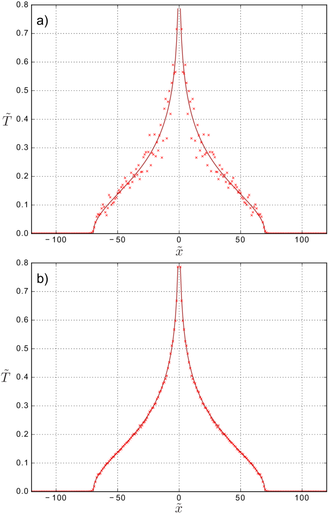
Figure 2: Comparing the analytical solution (6.8) for a crystal without viscous environment (the brown solid line) and the numerical solution (the red crosses) in the case $N=1000$, $\tilde{t}=70$. a) $R=100$, b) $R=10000$.

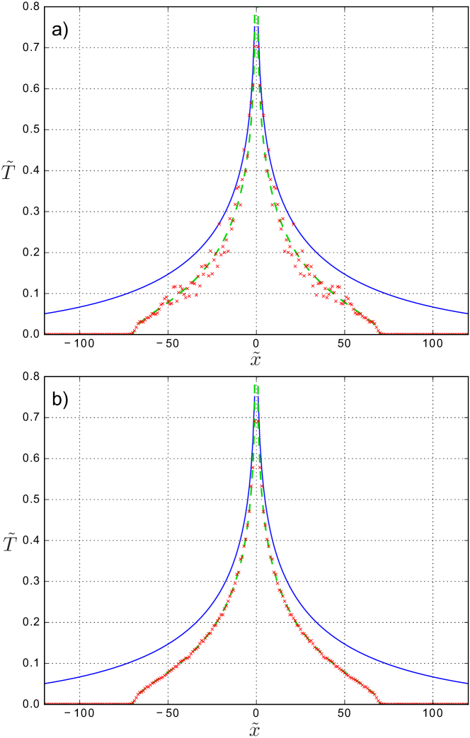
Figure 3: Comparing the unsteady analytical solution (6.7) for a crystal in a viscous environment (the green dashed line), the corresponding steady-state analytical solution (6.9) in the form of the Macdonald function (the blue solid line), and the numerical solution (the red crosses) in the case $\tilde{\eta}=0.01$, $N=1000$, $\tilde{t}=70$. a) $R=100$, b) $R=10000$.

Figure 2 corresponds to a crystal without viscous environment. Figure 3 correspond to a crystal in a viscous environment in the case where $\tilde{t}=70$ is small enough for the solution to be regarded as an unsteady one. Figure 4 correspond to a crystal in a viscous environment in the case where $\tilde{t}=500$ is large enough for the solution to be regarded as a steady-state one. All figures are presented for two numbers of realizations: a) $R=100$ and b) $R=10000$. One can see that in all cases, for sufficiently large $R=10000$ the analytical and numerical solutions are in a very good agreement.

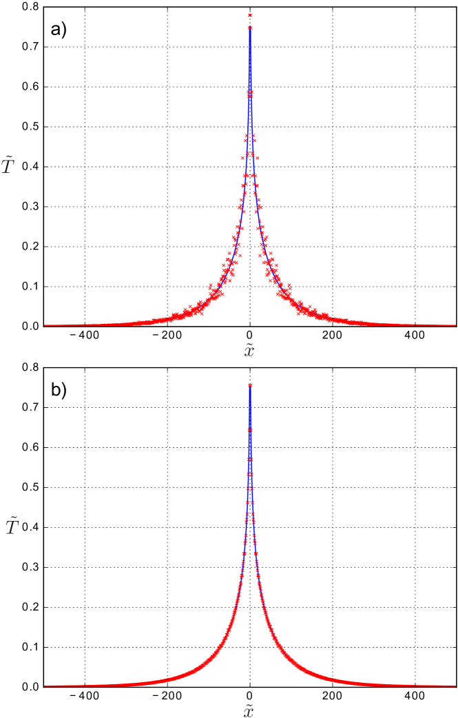
Figure 4: Comparing the steady-state analytical solution (6.9) in the form of the Macdonald function (the blue solid line) and the numerical solution (the red crosses) in the case $\tilde{\eta}=0.01$, $N=1000$, $\tilde{t}=500$. a) $R=100$, b) $R=10000$.

7 Comparison with the Fourier thermal conductivity

Let us compare our results with the classical results obtained in the framework of the heat equation based on Fourier’s law. Consider the case of the non-stationary temperature distribution caused by a suddenly applied point source of heat supply. For a crystal in an environment, the solution is given by formula (5.27). For large times, there exists a steady-state solution (see (5.28)), in contrast to the case $\eta=0$ of a crystal without environment, where the solution (5.17) of the same problem grows logarithmically. The dimensionless forms of solutions (5.27), (5.28), (5.17) are (6.7), (6.9), (6.8), respectively.

Introducing the dimensionless quantities $\tilde{t},\ \tilde{T},\tilde{x}$ according to (6.2), (6.5), and (6.10), respectively, the classical heat equation in the case under consideration can be formulated in the following form

$$\frac{\partial\tilde{T}}{\partial\tilde{t}}-\varkappa\frac{\partial^{2}\tilde{T}}{\partial^{2}\tilde{x}}=\lambda H(\tilde{t})\delta(\tilde{x}),$$ (7.1)

where $\varkappa,\ \lambda$ are positive dimensionless constants. The solution of (7.1) that equals zero for $\tilde{t}<0$ is (see Vladimirov1971 )

$$\tilde{T}=\frac{\lambda H(\tilde{t})}{2\sqrt{\varkappa\pi}}\int_{0}^{\tilde{t}}\frac{\exp\left(-\frac{|\tilde{x}|^{2}}{4\varkappa\tau}\right)}{\sqrt{\tau}}\,d\tau\\ =\lambda H(\tilde{t})\left(\sqrt{\frac{\tilde{t}}{\pi\varkappa}}\exp\left(-\frac{\tilde{x}^{2}}{4\varkappa\tilde{t}}\right)-\frac{|\tilde{x}|}{2\varkappa}\operatorname{erfc}\frac{|\tilde{x}|}{2\sqrt{\mathstrut\varkappa\tilde{t}}}\right).$$ (7.2)

For $\tilde{t}\to\infty$ the right-hand side of (7.2) grows proportionally to $\sqrt{\tilde{t}}$ being bounded at $\tilde{x}=0$.

Now we want to compare qualitatively the solutions (6.7) or (6.8) from the one hand, and (7.2) from the other hand. At first, we need to choose the reasonable values for material constants $\varkappa$ and $\lambda$ in (7.2). In order to make the solutions corresponding to different physical models more similar in some sense, for certain $\tilde{t}=\tilde{t}_{0}$ we take constants $\varkappa=\varkappa_{0}(\tilde{t}_{0})$ and $\lambda=\lambda_{0}(\tilde{t}_{0})$ such that the following pairs of the quantities

$$\int_{-\infty}^{\infty}\tilde{T}(\tilde{x},\tilde{t}_{0})\,d\tilde{x}\quad\text{and}\quad\int_{-\infty}^{\infty}\tilde{x}^{2}\tilde{T}(\tilde{x},\tilde{t}_{0})\,d\tilde{x}$$ (7.3)

calculated by virtue of (6.8) and (7.2), respectively, are mutually equal. In such a way we get that $\lambda_{0}=1/2$ and does not depend on $\tilde{t}_{0}$, while the quantity $\varkappa_{0}$ depends on $\tilde{t}_{0}$.

The comparison between unsteady solutions for the crystal and the solution of the heat equation is given in Figure 5 (all plots are calculated for $\tilde{t}_{0}=30$).

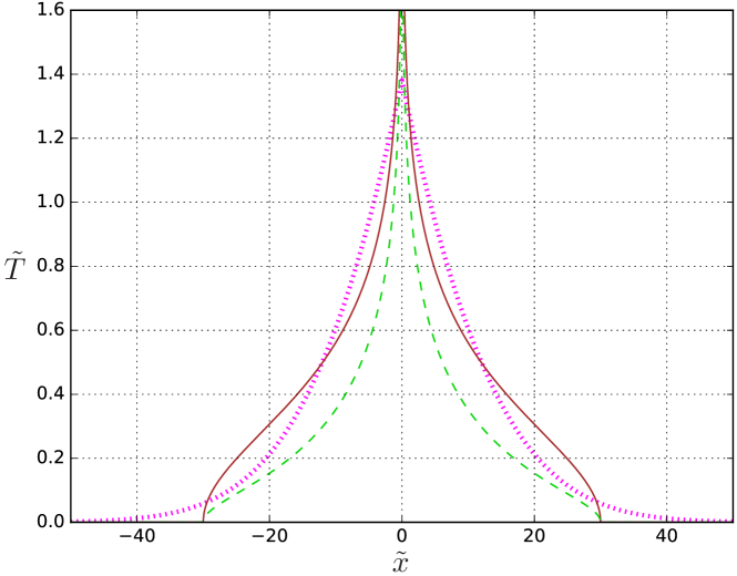
Figure 5: A qualitative comparison between the non-stationary analytical solution (6.7) for a crystal in a viscous environment ($\tilde{\eta}=0.03$, the green dashed line), the non-stationary analytical solution (6.8) for a crystal without viscous environment (the brown solid line), and the solution (7.2) of the heat equation ($\varkappa=5.00$, the magenta dotted line).

Certainly, the most important difference here is that according to (6.7) & (6.8) the heat propagates at a finite speed. Both solutions for the crystal are unbounded at $x=0$, while the solution of the heat equation (7.2) remains to be finite.

8 Conclusion

In the paper, we started with equations (2.1) for stochastic dynamics of a one-dimensional harmonic crystal in a viscous environment. We introduced in the standard way the kinetic temperature in the crystal as a quantity proportional to the statistical dispersion of the particle velocities. The most important results of the paper are the differential-difference equation (4.9) for the heat propagation in the crystal and the analytical formulas (5.17), (5.25), and (5.28) describing the ballistic heat propagation in the crystal from a point heat source. Formula (5.17) gives the non-stationary kinetic temperature distribution in a crystal without viscous environment caused by a point source of constant intensity. Formulas (5.25) and (5.28) correspond to the case of a crystal in a viscous environment. Formula (5.25) gives the non-stationary kinetic temperature distribution caused by a point pulse source (i.e., the fundamental solution). Formula (5.28) shows that the steady-state kinetic temperature distribution caused by a point source of constant intensity is described by the Macdonald function of zero order. The comparison between numerical solution of equations (2.1) and analytic solution of differential-difference equation (4.9) demonstrates a good agreement (see Figures 2–4). In the case of the heat source of general structure the formula for the kinetic temperature can be obtained as the convolution of the heat source function with the corresponding fundamental solution (see Eqs. (5.18), (5.31)).

A comparison of our results with the classical model based on the heat equation and Fourier’s law demonstrates an essential difference in the kinetic temperature distribution near a point source of heat supply (see Section 7 and Fig. 5). In the framework of our model the heat propagates at the speed of sound for the crystal. We expect that the results obtained in the paper can be used to describe the heat transfer in low-dimensional nanostructures and ultra-pure materials chang2008breakdown ; xu2014length ; goldstein2007mechanics . On the other hand, we expect that the theoretical result expressed by formula (5.28) can be verified by experiments with laser excitation of nanostructures.

Appendix A The derivation of the dynamic equations for the covariances

Consider a system of stochastic differential equations

$$dx_{i}=a_{i}(\mathbf{x},t)\,dt+\sum_{\alpha}b_{i\alpha}(\mathbf{x},t)\,dW_{\alpha}\,,\qquad i=1,...,n,$$ (A.1)

where $\mathbf{x}=[x_{1},\dots,x_{n}]^{\top}$ and $W_{\alpha}$ is a vector of uncorrelated Wiener variables. According to stepanov2013stochastic (Chapter 6, formulas (6.4)–(6.17)), it follows from the Itô lemma that the following equation for the covariance variables holds:

$$\left\langle x_{p}x_{q}\right\rangle^{\cdot}=\left\langle x_{p}a_{q}+x_{q}a_{p}+b_{q\alpha}b_{p\alpha}\right\rangle.$$ (A.2)

In the particular case (2.1), we have $b_{i\alpha}(\mathbf{x},t)=\delta_{\alpha i}b_{i}(\mathbf{x},t)$, whence

$$\langle{x_{p}x_{q}}\rangle^{\cdot}=\langle{x_{p}a_{q}+x_{q}a_{p}}\rangle+\delta_{pq}\langle{b_{p}b_{q}}\rangle.$$ (A.3)

Now we apply (A.3) to (2.1) and obtain

$$\begin{gathered}\langle{u_{p}u_{q}}\rangle^{\cdot}=\langle{u_{p}v_{q}}\rangle+\langle{v_{p}u_{q}}\rangle,\\ \langle{u_{p}v_{q}}\rangle^{\cdot}=\langle{u_{p}F_{q}}\rangle+\langle{v_{p}v_{q}}\rangle,\\ \langle{v_{p}v_{q}}\rangle^{\cdot}=\langle{v_{p}F_{q}}\rangle+\langle{F_{p}v_{q}}\rangle+\delta_{pq}\langle{b_{p}b_{q}}\rangle.\end{gathered}$$ (A.4)

Applying these formulas to the particular case where $F_{i}$ are given by Eq. (2.2) yields formula (2.11).

Appendix B Some identities of the calculus of finite differences

Consider an infinite sequence $f_{p}$, where $p$ is an arbitrary integer. Introduce the left and right shift operators $h$ and $\nu$, respectively:

$$hf_{p}\stackrel{{\scriptstyle\mbox{\scriptsize def}}}{{=}}f_{p+1}\,,\qquad\nu f_{p}\stackrel{{\scriptstyle\mbox{\scriptsize def}}}{{=}}f_{p-1}.$$ (B.1)

Clearly,

$$h\nu=1\qquad\Longleftrightarrow\qquad\nu=h^{-1}.$$ (B.2)

One has

$${\cal L}=h+\nu-2,$$ (B.3)

$$\mathscr{D}=h-\nu.$$ (B.4)

By definition, put

$$\varSigma\stackrel{{\scriptstyle\mbox{\scriptsize def}}}{{=}}h+\nu+2={\cal L}+4.$$ (B.5)

One has

$${\cal L}\varSigma f_{p}=f_{p+2}-2f_{p}+f_{p-2}=\mathscr{D}^{2}f_{p}.$$ (B.6)

Introduce the sign change operator $(-1)^{p}$. One has

$$h(-1)^{p}=(-1)^{p+1}h,$$ (B.7)

$$\nu(-1)^{p}=(-1)^{p+1}\nu,$$ (B.8)

$${\cal L}(-1)^{p}=(-1)^{p+1}\varSigma,$$ (B.9)

$$\varSigma=(-1)^{p+1}{\cal L}(-1)^{p}.$$ (B.10)

References

- (1) Rieder, Z., Lebowitz, J., Lieb, E.: Properties of a harmonic crystal in a stationary nonequilibrium state. Journal of Mathematical Physics 8(5), 1073–1078 (1967)
- (2) Bonetto, F., Lebowitz, J., Rey-Bellet, L.: Fourier’s law: A challenge to theorists. In: A. Fokas, A. Grigoryan, T. Kibble, B. Zegarlinski (eds.) Mathematical physics 2000. World Scientific (2000)
- (3) Lepri, S., Livi, R., Politi, A.: Thermal conduction in classical low-dimensional lattices. Physics reports 377(1), 1–80 (2003)
- (4) Lepri, S., Livi, R., Politi, A.: On the anomalous thermal conductivity of one-dimensional lattices. Europhysics Letters 43(3), 271 (1998)
- (5) Dhar, A.: Heat transport in low-dimensional systems. Advances in Physics 57(5), 457–537 (2008)
- (6) Lepri, S.: Thermal transport in low dimensions: from statistical physics to nanoscale heat transfer. Springer (2016)
- (7) Casati, G., Ford, J., Vivaldi, F., Visscher, W.: One-dimensional classical many-body system having a normal thermal conductivity. Physical review letters 52(21), 1861–1864 (1984)
- (8) Aoki, K., Kusnezov, D.: Bulk properties of anharmonic chains in strong thermal gradients: non-equilibrium theory. Physics Letters A 265(4), 250–256 (2000)
- (9) Gendelman, O., Savin, A.: Normal heat conductivity in chains capable of dissociation. Europhysics Letters 106(3), 34,004 (2014)
- (10) Savin, A., Kosevich, Y.: Thermal conductivity of molecular chains with asymmetric potentials of pair interactions. Physical Review E 89(3), 032,102 (2014)
- (11) Gendelman, O., Savin, A.: Heat conduction in a chain of colliding particles with a stiff repulsive potential. Physical Review E 94(5), 052,137 (2016)
- (12) Spohn, H.: Fluctuating hydrodynamics approach to equilibrium time correlations for anharmonic chains. In: S. Lepri (ed.) Thermal transport in low dimensions: from statistical physics to nanoscale heat transfer, Lecture Notes in Physics, pp. 107–158. Springer (2016)
- (13) Bonetto, F., Lebowitz, J., Lukkarinen, J.: Fourier’s law for a harmonic crystal with self-consistent stochastic reservoirs. Journal of statistical physics 116(1), 783–813 (2004)
- (14) Le-Zakharov, A., Krivtsov, A.: Molecular dynamics investigation of heat conduction in crystals with defects. Doklady Physics 53(5), 261–264 (2008)
- (15) Chang, C., Okawa, D., Garcia, H., Majumdar, A., Zettl, A.: Breakdown of Fourier’s law in nanotube thermal conductors. Physical review letters 101(7), 075,903 (2008)
- (16) Xu, X., Pereira, L., Wang, Y., Wu, J., Zhang, K., Zhao, X., Bae, S., Bui, C., Xie, R., Thong, J., Hong, B., Loh, K., Donadio, D., Li, B., Özyilmaz, B.: Length-dependent thermal conductivity in suspended single-layer graphene. Nature communications 5 (2014)
- (17) Hsiao, T., Huang, B., Chang, H., Liou, S., Chu, M., Lee, S., Chang, C.: Micron-scale ballistic thermal conduction and suppressed thermal conductivity in heterogeneously interfaced nanowires. Physical Review B 91(3), 035,406 (2015)
- (18) Cahill, D., Ford, W., Goodson, K., Mahan, G., Majumdar, A., Maris, H., Merlin, R., Phillpot, S.: Nanoscale thermal transport. Journal of Applied Physics 93(2), 793–818 (2003)
- (19) Liu, S., Xu, X., Xie, R., Zhang, G., Li, B.: Anomalous heat conduction and anomalous diffusion in low dimensional nanoscale systems. The European Physical Journal B 85(337) (2012)
- (20) Chang, C.: Experimental probing of non-Fourier thermal conductors. In: S. Lepri (ed.) Thermal transport in low dimensions: from statistical physics to nanoscale heat transfer, Lecture Notes in Physics, vol. 921, pp. 305–338. Springer (2016)
- (21) Peierls, R.: Quantum theory of solids. Oxford University Press (1955)
- (22) Ziman, J.: Electrons and phonons: the theory of transport phenomena in solids. Oxford University Press (1960)
- (23) Hsiao, T., Chang, H., Liou, S., Chu, M., Lee, S., Chang, C.: Observation of room-temperature ballistic thermal conduction persisting over 8.3 m in SiGe nanowires. Nature nanotechnology 8(7), 534–538 (2013)
- (24) Kannan, V., Dhar, A., Lebowitz, J.: Nonequilibrium stationary state of a harmonic crystal with alternating masses. Physical Review E 85(4), 041,118 (2012)
- (25) Dhar, A., Dandekar, R.: Heat transport and current fluctuations in harmonic crystals. Physica A 418, 49–64 (2015)
- (26) Allen, K., Ford, J.: Energy transport for a three-dimensional harmonic crystal. Physical Review 187(3), 1132 (1969)
- (27) Nakazawa, H.: On the lattice thermal conduction. Progress of Theoretical Physics Supplement 45, 231–262 (1970)
- (28) Lee, L., Dhar, A.: Heat conduction in a two-dimensional harmonic crystal with disorder. Physical review letters 95(9), 094,302 (2005)
- (29) Kundu, A., Chaudhuri, A., Roy, D., Dhar, A., Lebowitz, J., Spohn, H.: Heat conduction and phonon localization in disordered harmonic crystals. Europhysics Letters 90(4), 40,001 (2010)
- (30) Dhar, A., Saito, K.: Heat transport in harmonic systems. In: S. Lepri (ed.) Thermal transport in low dimensions: from statistical physics to nanoscale heat transfer, Lecture Notes in Physics, vol. 921, pp. 39–106. Springer (2016)
- (31) Bernardin, C., Kannan, V., Lebowitz, J., Lukkarinen, J.: Harmonic systems with bulk noises. Journal of Statistical Physics 146(4), 800–831 (2012)
- (32) Freitas, N., Paz, J.: Analytic solution for heat flow through a general harmonic network. Physical Review E 90(4), 042,128 (2014)
- (33) Freitas, N., Paz, J.: Erratum: Analytic solution for heat flow through a general harmonic network. Physical Review E 90(6), 069,903 (2014)
- (34) Hoover, W., Hoover, C.: Hamiltonian thermostats fail to promote heat flow. Communications in Nonlinear Science and Numerical Simulation 18(12), 3365–3372 (2013)
- (35) Lukkarinen, J., Marcozzi, M., Nota, A.: Harmonic chain with velocity flips: thermalization and kinetic theory. Journal of Statistical Physics 165(5), 809–844 (2016)
- (36) Gendelman, O., Shvartsman, R., Madar, B., Savin, A.: Nonstationary heat conduction in one-dimensional models with substrate potential. Physical Review E 85(1), 011,105 (2012)
- (37) Tsai, D., MacDonald, R.: Molecular-dynamical study of second sound in a solid excited by a strong heat pulse. Physical Review B 14(10), 4714 (1976)
- (38) Ladd, A., Moran, B., Hoover, W.: Lattice thermal conductivity: A comparison of molecular dynamics and anharmonic lattice dynamics. Physical Review B 34(8), 5058 (1986)
- (39) Volz, S., Saulnier, J.B., Lallemand, M., Perrin, B., Depondt, P., Mareschal, M.: Transient Fourier-law deviation by molecular dynamics in solid argon. Physical review B 54(1), 340 (1996)
- (40) Daly, B., Maris, H., Imamura, K., Tamura, S.: Molecular dynamics calculation of the thermal conductivity of superlattices. Physical review B 66(2), 024,301 (2002)
- (41) Gendelman, O., Savin, A.: Nonstationary heat conduction in one-dimensional chains with conserved momentum. Physical Review E 81(2), 020,103 (2010)
- (42) Babenkov, M., Krivtsov, A., Tsvetkov, D.: Energy oscillations in a one-dimensional harmonic crystal on an elastic substrate. Physical Mesomechanics 19(3), 282–290 (2016)
- (43) Krivtsov, A.: Heat transfer in infinite harmonic one-dimensional crystals. Doklady Physics 60(9), 407–411 (2015)
- (44) Krivtsov, A.: Energy oscillations in a one-dimensional crystal. Doklady Physics 59(9), 427–430 (2014)
- (45) Hoover, W., Hoover, C.: Simulation and Control of Chaotic Nonequilibrium Systems. World Scientific (2015)
- (46) Krivtsov, A.: From nonlinear oscillations to equation of state in simple discrete systems. Chaos, Solitons & Fractals 17(1), 79–87 (2003)
- (47) Berinskii, I.: Elastic networks to model auxetic properties of cellular materials. International Journal of Mechanical Sciences 115, 481–488 (2016)
- (48) Kuzkin, V., Krivtsov, A., Podolskaya, E., Kachanov, M.: Lattice with vacancies: elastic fields and effective properties in frameworks of discrete and continuum models. Philosophical Magazine 96(15), 1538–1555 (2016)
- (49) Berinskii, I., Krivtsov, A.: Linear oscillations of suspended graphene. In: Shell and Membrane Theories in Mechanics and Biology, pp. 99–107. Springer (2015)
- (50) Berinskii, I., Krivtsov, A.: A hyperboloid structure as a mechanical model of the carbon bond. International Journal of Solids and Structures 96, 145–152 (2016)
- (51) Shishkina, E., Gavrilov, S.: A strain-softening bar with rehardening revisited. Mathematics and Mechanics of Solids 21(2), 137–151 (2016)
- (52) Gavrilov, S.: Dynamics of a free phase boundary in an infinite bar with variable cross-sectional area. ZAMM — Journal of Applied Mathematics and Mechanics / Zeitschrift für Angewandte Mathematik und Mechanik 87(2), 117–127 (2007)
- (53) Gavrilov, S., Shishkina, E.: On stretching of a bar capable of undergoing phase transitions. Continuum Mechanics and Thermodynamics 22, 299–316 (2010)
- (54) Gavrilov, S., Shishkina, E.: A strain-softening bar revisited. ZAMM — Journal of Applied Mathematics and Mechanics / Zeitschrift für Angewandte Mathematik und Mechanik 95(12), 1521–1529 (2015)
- (55) Shishkina, E., Gavrilov, S.: Stiff phase nucleation in a phase-transforming bar due to the collision of non-stationary waves. Archive of Applied Mechanics 87(6), 1019–1036 (2017)
- (56) Gavrilov, S., Herman, G.: Wave propagation in a semi-infinite heteromodular elastic bar subjected to a harmonic loading. Journal of Sound and Vibration 331(20), 4464–4480 (2012)
- (57) Krivtsov, A.: On heat transfer in a thermally perturbed harmonic chain. arXiv:1709.07924 (2017)
- (58) Chandrasekharalah, D.: Thermoelasticity with second sound: a review. Appl. Mech. Rev. 39(3), 355 (1986)
- (59) Tzou, D.: Macro-to microscale heat transfer: the lagging behavior. John Wiley & Sons (2014)
- (60) Cattaneo, C.: Sur une forme de l’équation de la chaleur éliminant le paradoxe d’une propagation instantanée. Comptes Rendus de L’Academie des Sciences 247(4), 431–433 (1958)
- (61) Vernotte, P.: Les paradoxes de la théorie continue de léquation de la chaleur. Comptes Rendus de L’Academie des Sciences 246(22), 3154–3155 (1958)
- (62) Kuzkin, V., Krivtsov, A.: An analytical description of transient thermal processes in harmonic crystals. Physics of the Solid State 59(5), 1051–1062 (2017)
- (63) Kuzkin, V., Krivtsov, A.: Fast and slow thermal processes in harmonic scalar lattices. Journal of Physics: Condensed Matter 29(50), 505,401 (2017)
- (64) Indeitsev, D., Osipova, E.: A two-temperature model of optical excitation of acoustic waves in conductors. Doklady Physics 62(3), 136–140 (2017)
- (65) Andrews, L.: Special Functions of Mathematics for Engineers. SPIE Publications (1997)
- (66) Kloeden, P., Platen, E.: Numerical solution of stochastic differential equations. Springer (1999)
- (67) Stepanov, S.: Stochastic world. Springer (2013)
- (68) Langevin, P.: Sur la théorie du mouvement brownien. Comptes Rendus de L’Academie des Sciences 146(530-533), 530 (1908)
- (69) Lemons, D., Gythiel, A.: Paul Langevin’s 1908 paper “On the theory of Brownian motion”[“Sur la théorie du mouvement brownien”], CR Acad. Sci.(Paris) 146, 530–533 (1908)]. American Journal of Physics 65(11), 1079–1081 (1997)
- (70) Krivtsov, A.: Dynamics of heat processes in one-dimensional harmonic crystals. In: Problems of mathematical physics and applied mathematics: Proceedings of the Seminar in Honor of Prof. E.A. Tropp’s 75th Anniversary, pp. 63–81. Ioffe Institute, St. Petersburg (2016). In Russian
- (71) Vladimirov, V.: Equations of Mathematical Physics. Marcel Dekker, New York (1971)
- (72) Lepri, S., Mejía-Monasterio, C., Politi, A.: Nonequilibrium dynamics of a stochastic model of anomalous heat transport. Journal of Physics A 43(6), 065,002 (2010)
- (73) Nayfeh, A.: Perturbation methods. John Wiley & Sons (2008)
- (74) Krivtsov, A.: On unsteady heat conduction in a harmonic crystal. arXiv:1509.02506 (2015)
- (75) Brigham, E.: The fast Fourier transform and its applications. Prentice Hall (1974)
- (76) Slepyan, L., Yakovlev, Y.: Integral transform in non-stationary problems of mechanics. Sudostroenie (1980). In Russian
- (77) Gel’fand, I., Shilov, G.: Generalized Functions. Volume I: Properties and Operations. Academic Press, New York (1964)
- (78) Polyanin, A.: Handbook of linear partial differential equations for engineers and scientists. Chapman & Hall/CRC (2002)
- (79) Prudnikov, A., Brychkov, Y., Marichev, O.: Integrals and Series, Vol. 1, Elementary Functions. Gordon & Breach, New York (1986)
- (80) Aleixo, R., Oliveira, E.: Green’s function for the lossy wave equation. Revista Brasileira de Ensino de Fisica 30(1), 1302 (2008)
- (81) Goldstein, R., Morozov, N.: Mechanics of deformation and fracture of nanomaterials and nanotechnology. Physical Mesomechanics 10(5-6), 235–246 (2007)