Quadrupolar power radiation by a binary system in de Sitter background

Abstract

Cosmological observations over past couple of decades favor our universe with a tiny positive cosmological constant. Presence of cosmological constant not only imposes theoretical challenges in gravitational wave physics, it has also observational relevance. Inclusion of cosmological constant in linearized theory of gravitational waves modifies the power radiated quadrupole formula. There are two types of observations which can be impacted by the modified quadrupole formula. One is the orbital decay of an inspiraling binary and other is the modification of the waveform at the detector. Modelling a compact binary system in an elliptic orbit on de Sitter background we obtain energy and angular momentum radiation due to emission of gravitational waves. We also investigate evolution of orbital parameters under back reaction and its impact on orbital decay rate. In the limit to circular orbit our result matches to that obtained in ref. Bonga .

I Introduction

Two years after the completion of general relativity, in 1918, Einstein derived power radi- ated quadrupole formula in Minkowski background. Einstein’s quadrupole formula was the first quantitative estimate of the power radiated in the form of gravitational radiation. It was also shown that to the leading order the emitted power due to gravitational radiation is proportional to the square of the third derivative of mass quadrupole moment of the source Einstein . This power loss would cause binary system to shrink slowly. Such a secular change in the orbital period of Hulse-Taylor binary pulsar was confirmed by observation to the accuracy of $10^{-3}$, thereby providing an indirect affirmation of gravitational waves TaylorI ; TaylorII ; Damour . Einstein’s theory also passed with flying colors in the direct observation of newly opened gravitational wave astronomy - gravitational wave template predicted by Einstein’s theory matches with observed signal GWI ; GWII ; GWIII ; GWIV .

All these theoretical frameworks assume a vanishing cosmological constant. However, by now cosmological observations (e.g. red shift of type Ia supernovae) have established that our universe favors a positive cosmological constant ($\Lambda$). Inclusion of cosmological constant not only posits theoretical challenges, it could also potentially provide an independent estimate of $\Lambda$ from the current accuracy of observation. It is natural to ask how does the presence of cosmological constant affect orbital decay of a binary system. Change in orbital decay also induces a change in orbital phase which is sensitive to current gravitational wave detectors. The aim of this work is to get an estimate of quadrupolar power loss by an elliptic binary system in de Sitter background. A priori the order of magnitude of corrections over Minkowski background is not clear. Even if it is negligible, it needs to be demonstrated as there are many conceptual and technical difficulties in the theory of gravitational waves in de Sitter space-time compared to Minkowski space-time. This work is a part of AA’s M.Sc. thesis Ankit and the case of circular orbit has been discussed in JH’s Ph.D. thesis Jahanur .

While it is well recognized that there is no tensorial (which is both local and generally covariant) definition of stress tensor for gravitational field, it is possible to construct meaningful, quasi-local quantities to represent total energy/momentum in specific contexts. One of the earliest such proposals is by Isaacson tailored for the context in which there are two widely separated spatio-temporal scales. For sources which are rapidly varying (relative to the length scale set by cosmological constant), there is an identification of gravitational waves as ripple on a background within the so called ‘short wave approximation’. Let $L_{B}$ denote the length scale of variation of the background and $\lambda$ the length scale of the ripple with $\lambda\ll L_{B}$. In this context Isaacson defined an effective gravitational stress tensor for the ripples which is gauge invariant to leading order in the ratio of the two scales Isaacson . In a recent paper DateJH2 co-authored by one of the authors of this paper, it has been discussed how Isaacson prescription can be adapted to compute quadrupolar power, radiated by a rapidly varying compact source in de Sitter background. Quadrupole formula on de Sitter background can also be obtained using covariant phase formalism ABKII ; ABKIII ; JHIII . It exploits the phase space structure of the space of linearized solutions and defines a gauge invariant and conserved charges corresponding to the isometries of de Sitter background. Compact binary system is the natural test-bed to apply the new quadrupole formula.

This paper is organized as follows. In section II, we recall the power radiated quadrupole formula from DateJH2 . The modified quadrupole formula involves mass quadrupole moment as well as pressure quadrupole moment of the source. As for non-relativistic (weakly stressed) compact source we can neglect the pressure term, in section III, we discuss the derivation of mass quadrupole moment of a point particle in de Sitter background. In section IV, we spell out the assumptions made to model an elliptic binary in de Sitter background. Given these assumptions, the quadrupolar energy flux radiated by an elliptic binary system is presented in section V, while section VI contains a discussion of angular momentum loss . In section VII, we discuss decay of orbital parameters due to energy and angular momentum loss. This is a new result. The final section IX concludes with a summary and discussion. Some of the technical details are given in an appendix. We set $c=1$ throughout.

II Preliminaries

Cosmological observations over the decades have indicated that our universe is undergoing an accelerated expansion, which is most simply modelled by a positive cosmological constant. In this light, the weak gravitational field should be re-looked at as ripples on the de Sitter background. To compute quadrupolar power radiation due to a elliptic binary system in de Sitter background we follow the framework developed in DateJH2 . In this section we review the work and give relevant expressions.

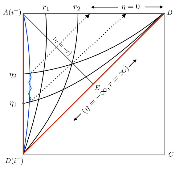
Figure 1: The full square is the Penrose diagram of de Sitter space-time with generic point representing a 2-sphere. The blue line denotes trajectory of spatially compact source in de Sitter background. ABD part is the the future Poincaré patch, covered by the conformal chart $(\eta,r,\theta,\phi)$. The line AB denotes the future null infinity, $\mathcal{J}^{+}$ while the line AE denotes the cosmological horizon, $\mathcal{H}^{+}$. Two constant $\eta$ space-like hypersurfaces are shown with $\eta_{2}>\eta_{1}$. The two constant $r$, time-like hypersurfaces have $r_{2}>r_{1}$. The two dotted lines denote the out-going null rays emanating from $\eta=\eta_{1},\eta_{2}$ on the world line through the source.

The de Sitter space-time defined as the hyperboloid in five dimensional Minkowski space- time, has a conformal chart of coordinates ($\eta,r,\theta,\phi$), as shown in figure 1. To be definite, let us take the world-tube of the spatially compact source to be around the line AD for all times. In this case source world-tube has future and past time-like infinity, denoted by $i^{\pm}$. Causal future of the compact source is only the future Poincaré patch (ABD) of full de Sitter. No observer whose world-line is confined to the past Poincaré patch (BCD) can detect the radiation emitted by the gravitating source. Therefore, to study gravitational radiation due to compact sources, it is sufficient to restrict oneself to future Poincaré Patch rather than full de Sitter space-time DateJHI ; ABKII . There are two natural coordinate charts for the future Poincaré patch, i.e., a conformal chart: $(\eta,x^{i})$ and a cosmological chart: $(t,x^{i})$. In the conformal chart ($\eta,x^{i})$ the background de Sitter metric takes the form,

$$ds^{2}=~{}a^{2}(\eta)~{}\bigg{[}-d\eta^{2}+\sum_{i}(dx^{i})^{2}\bigg{]}\ ,~{}~{}a(\eta)=-(H\eta)^{-1}~{},~{}\eta\in(-\infty,0)~{},~{}H:=\sqrt{\frac{\Lambda}{3}}.$$ (1)

While conformal coordinates are convenient in detailed calculations of gravitational perturbations, they are not suitable for taking the limit $\Lambda\rightarrow 0$ ABKIII . To take that limit we have to use proper time $t$, which is related to conformal time $\eta$ via $\eta:=-H^{-1}e^{-Ht}$. In these coordinates ($t,x^{i}$), line element becomes,

$$ds^{2}=-dt^{2}+e^{2Ht}\sum_{i=2}^{4}(dx^{i})^{2}$$ (2)

Poincaré patch has seven dimensional symmetry group - 3 spatial rotations, 3 spatial translations and 1 time translation. For computing power radiated quadrupole formula in de Sitter background, it suffices to focus on the time translational Killing field. In order to find the Killing vector field of time translations we let $t\rightarrow t+\delta t$ in the above metric. This leads to

$$ds^{2}\rightarrow-dt^{2}+e^{2Ht}(1+2H~{}\delta t)\sum_{i=2}^{4}(dx^{i})^{2}$$ (3)

To make the metric invariant under this time translation, the spatial coordinates, $x^{i}$, must be transformed as $x^{i}\rightarrow x^{i}-Hx^{i}\delta t$. In general, a Killing vector $\xi^{\alpha}$ is an infinitesimal generator of isometry, i.e., for $x^{\alpha}\rightarrow x^{\alpha}+\epsilon\xi^{\alpha}$, the metric remains invariant. Identifying $\epsilon=\delta t$, the Killing vector which generates time translation in the cosmological coordinate system is $T^{\mu}=(1,-Hx^{i})$. We will work with this time-translational Killing field to compute quadrupolar radiation.

We briefly recall the derivation of quadrupole formula in de Sitter background from DateJH2 . Under the ‘short wavelength approximation’ for rapidly varying compact source, we visualize gravitational waves as high frequency ripple over a slowly varying background space-time. Let $L_{B}$ be the length scale variation of background and $\lambda$ be the length scale of ripple. In the present context of de Sitter background, $L_{B}$ length scale is set by the cosmological constant, $L_{B}\sim\frac{1}{\sqrt{\Lambda}}$. To maintain a clear cut separation between background and ripple for all time, we demand that $\lambda\ll L_{B}$. In this context, it is possible to define Isaacson effective gravitational stress tensor, $t_{\mu\nu}$ for the ripples . To obtain Isaacson stress tensor, one begins with an expansion of the form $g_{\mu\nu}=\bar{g}_{\mu\nu}+\epsilon h_{\mu\nu}$ and writes the Einstein equation in source free region as,

$$R_{\mu\nu}(\bar{g}+\epsilon h) = \Lambda(\bar{g}_{\mu\nu}+\epsilon h_{\mu\nu})$$

$$\therefore R^{(0)}_{\mu\nu}(\bar{g})+\epsilon R^{(1)}_{\mu\nu}(\bar{g},h)+\epsilon^{2}R^{(2)}_{\mu\nu}(\bar{g},h) = \Lambda(\bar{g}_{\mu\nu}+\epsilon h_{\mu\nu})$$ (4)

Introduce an averaging over an intermediate scale $\ell$, $\lambda\ll\ell\ll L_{B}$, which satisfies the properties: (i) average of odd powers of $h$ vanishes and (ii) average of space-time divergence of tensors is sub-leading to the ratio of two length scales, $\lambda/L_{B}$ MTW ; Stein . Taking the average of the above equation gives,

$$\langle R^{(0)}_{\mu\nu}\rangle+\epsilon^{2}\langle R^{(2)}_{\mu\nu}\rangle=\Lambda\bar{g}_{\mu\nu}.$$ (5)

Notice that $R^{(2)}$, which is quadratic in $h$, can have $L_{B}$ - scale variations and hence non-zero average. Thus it incorporates back reaction of ripple on the background and modifies the background equation as,

$$8\pi t_{\mu\nu} = \bar{R}_{\mu\nu}-\frac{1}{2}\bar{g}_{\mu\nu}\bar{R}+\Lambda\bar{g}_{\mu\nu}$$ (6)

This can be appropriately termed as ‘coarse-grained’ form of Einstein equation in source free region, where

$$t_{\mu\nu}(\bar{g},h) := ~{}-\frac{\epsilon^{2}}{8\pi}\left[\langle R^{(2)}_{\mu\nu}\rangle-\frac{1}{2}\bar{g}_{\mu\nu}\bar{g}^{\alpha\beta}\langle R^{(2)}_{\alpha\beta}\rangle\right]$$ (7)

is the effective stress-energy tensor of ripple. It should be noted that the stress tensor is symmetric and conserved with respect to background. Given a symmetric, conserved stress tensor and time-translational Killing vector of de Sitter background, one can construct conserved current $J^{\mu}_{T}:=-t^{\mu}_{\nu}~{}T^{\nu}$. From the conservation equation it follows,

$$0~{}=~{}\int_{\mathcal{V}}d^{4}x\sqrt{\bar{g}}\bar{\nabla}_{\mu}J_{\xi}^{\mu}=\int_{\mathcal{V}}d^{4}x\partial_{\mu}(\sqrt{\bar{g}}J_{\xi}^{\mu})=\int_{\partial\cal V}d\sigma_{\mu}J_{\xi}^{\mu},$$ (8)

For linearized retarded solution in de Sitter background, computing the energy flux ($\int_{\Sigma}d\sigma_{\mu}J^{\mu}_{T}$) integral across killing hypersurfaces, we obtain the power radiated quadrupole formula DateJH2 ,

$$\mathcal{P}~{}=~{}\frac{G}{8\pi}\int_{S^{2}}d^{2}s\langle\mathcal{Q}_{ij}^{tt}\mathcal{Q}^{ij}_{tt}\rangle$$ (9)

where, $\mathcal{Q}_{ij}:=\left[\mathcal{L}_{T}^{3}{Q}_{ij}+3H\mathcal{L}_{T}^{2}{Q}_{ij}+2H^{2}\mathcal{L}_{T}{Q}_{ij}+H\mathcal{L}_{T}^{2}{\bar{Q}}_{ij}+3H^{2}\mathcal{L}_{T}{\bar{Q}}_{ij}+2H^{3}\bar{Q}_{ij}\right](t_{ret})$ and $\mathcal{L}_{T}$ denotes Lie derivative with respect to time translational Killing vector. We would like to express this quantity in proper time coordinate $t$, of matter source. As moments are function of $t_{ret}$, using $\mathcal{L}_{T}:=\partial_{t}-2H$ on $Q_{ij}$ and $\bar{Q}_{ij}$, we can express $\mathcal{Q}_{ij}$ as,

$$\mathcal{Q}_{ij}=\left[\partial_{t}^{3}{Q}_{ij}-3H\partial_{t}^{2}{Q}_{ij}+2H^{2}\partial_{t}{Q}_{ij}+H\partial_{t}^{2}{\bar{Q}}_{ij}-H^{2}\partial_{t}{\bar{Q}}_{ij}\right](t_{ret}).$$ (10)

In these expressions, $Q_{ij}$ and $\bar{Q}_{ij}$ are mass quadrupole moment and pressure quadrupole moment respectively (see below), while $t_{ret}$ is defined as $\eta-r=-\frac{1}{H}~{}e^{-Ht_{ret}}$. The label tt denotes algebraically projected part of tensor field and is defined as $\mathcal{Q}_{ij}^{tt}:=\Lambda_{ij}^{kl}~{}\mathcal{Q}_{kl}$. $\Lambda_{ij}^{kl}$ is the algebraic projection operator which projects spatial components of a tensor to a plane orthogonal to radial direction and makes it traceless. The projection operator is defined as $\Lambda_{ij}^{kl}:=\frac{1}{2}(P_{i}^{k}P_{j}^{l}+P_{i}^{l}P_{j}^{k}-P_{ij}P^{kl}),\mbox{with}~{}P_{i}^{j}=\delta_{i}^{j}-\hat{x}_{i}\hat{x}^{j}$.

Let us take a quick detour to the definition of moments in de Sitter background. To maintain coordinate invariance and moment integrals to be well-defined, the moment variables must be coordinate scalars. The natural choice is to write moment variables in terms of tetrad components. The conformal form of de Sitter metric in eq. (1) suggests a natural choice DateJHI ,

$$f^{\alpha}_{~{}\underline{0}}~{}:=~{}-H\eta~{}(1,\vec{0})~{}~{},~{}~{}f^{\alpha}_{~{}\underline{m}}~{}:=~{}-H\eta\ \delta^{\alpha}_{~{}\underline{m}}\hskip 19.91684pt\Longleftrightarrow\hskip 19.91684ptf^{\alpha}_{~{}\underline{a}}:=-H\eta\delta^{\alpha}_{~{}\underline{a}}$$ (11)

The corresponding components of the stress tensor are given by, $\rho:=P_{\underline{00}}=T_{\alpha\beta}f^{\alpha}_{~{}\underline{0}}f^{\beta}_{~{}\underline{0}}~{}=~{}H^{2}\eta^{2}T_{00}\delta^{0}_{~{}\underline{0}}\delta^{0}_{~{}\underline{0}},P_{\underline{ij}}~{}:=~{}T_{\alpha\beta}f^{\alpha}_{~{}\underline{i}}f^{\beta}_{~{}\underline{j}}~{}=~{}H^{2}\eta^{2}T_{ij}\delta^{i}_{~{}\underline{i}}\delta^{j}_{~{}\underline{j}}\ ;\pi:=P_{\underline{ij}}\delta^{\underline{ij}}\ .$ The quadrupole moments of the two rotational scalars, $\rho,\pi$, are defined by integrating over the source distribution at $t=const.$ hypersurface,

$${Q}^{{i}{j}}(t) := \int_{Source(t)}d^{3}{x}\ a^{3}(t)\rho(t,\vec{x})~{}\bar{x}^{{i}}\bar{x}^{{j}}~{}~{},$$ (12)

$$\bar{Q}^{{i}{j}}(t) := \int_{Source(t)}d^{3}{x}\ a^{3}(t)\pi(t,\vec{x})~{}\bar{x}^{{i}}\bar{x}^{{j}}~{}.~{}$$ (13)

The determinant of the induced metric on $t=const.$ hypersurfaces is $a^{3}(t)$. The tetrad components of the moment variable are given by, $\bar{x}^{{i}}:=f^{\underline{i}}_{\alpha}x^{\alpha}=-(\eta H)^{-1}\delta^{{i}}_{~{}j}x^{j}=a(t)x^{{i}}$. It should be noted that the tetrad components measure the physical distance and $d^{3}x~{}a^{3}(t)=d^{3}\bar{x}$. Thus, effectively, moment variable is computed in a tetrad frame attached with source.

III Mass quadrupole moment of a point particle in de Sitter

To proceed let us investigate quadrupole moment of a point particle of mass $m$ in de Sitter background. For a compact, non-relativistic source, we can neglect pressure with respect to energy density and it is sufficient to compute only mass quadrupole moment. Let a point particle of mass $m$ is moving on a worldline $\gamma$ in a curved space-time with metric $g_{\alpha\beta}$. Action functional of the particle is given by Gravity ,

$$S_{p}=-m\int_{\gamma}\sqrt{-g_{\mu\nu}~{}\dot{x}^{\mu}\dot{x}^{\nu}}~{}d\sigma$$ (14)

where $\sigma$ is an arbitrary parameter along worldline of particle (which can be taken as proper time for convenience). We assume that the $m$ is small, so that perturbation $h_{\mu\nu}$ created by the particle can also be considered to be small. Now, as usual, decompose $g_{\mu\nu}=\bar{g}_{\mu\nu}+h_{\mu\nu}$. The background metric $\bar{g}_{\mu\nu}$ is independent of $m$ while the perturbation $h_{\mu\nu}$ contains dependence of $m$. To the leading order in $m$, particle’s energy-momentum tensor in background space-time is given by Poisson ; Straumann ,

$$T^{\mu\nu}=\frac{m}{\sqrt{-\bar{g}}}\int_{\gamma}u^{\mu}u^{\nu}\delta^{4}(x-x_{p})~{}d\tau$$ (15)

where $u^{\mu}$ denotes particle’s four velocity in background space-time and $x_{p}$ is the position of the particle. In conformal chart ($\eta,x^{i}$) of de Sitter background proper time, $d\tau=\sqrt{\bar{g}_{\mu\nu}~{}dx^{\mu}dx^{\nu}}=a\sqrt{\eta_{\mu\nu}~{}dx^{\mu}dx^{\nu}}=a~{}\gamma^{-1}d\eta$, where $\gamma^{-1}=\sqrt{1-(\frac{d\vec{x}}{d\eta})^{2}}$. For computing mass quadrupole moment, let us concentrate on $T^{00}$,

$$T^{00} =\frac{m}{a^{4}}\int\bigg{(}\frac{d\eta}{d\tau}\bigg{)}^{2}~{}\delta^{4}\big{(}x-x_{p}(\eta)\big{)}~{}\frac{d\tau}{d\eta}~{}d\eta$$ (16)

$$=\frac{m}{a^{5}}\gamma~{}\delta^{3}\big{(}\vec{x}-\vec{x}_{p}(\eta)\big{)}$$ (17)

$$\therefore T^{00} \approx\frac{m}{a^{5}}~{}\delta^{3}\big{(}\vec{x}-\vec{x}_{p}(\eta)\big{)}$$ (18)

In the last line we have dropped the Lorentz factor $\gamma$ assuming the source is non- relativistic. As the tetrad frame (11) is defined in ($\eta,x^{i}$) coordinates, we compute $\rho$ in conformal coordinates, after that we convert it in ($t,x^{i}$) coordinates. Hence,

$$\rho:=a^{-2}(\eta)T_{00}~{}\delta^{0}_{\underline{0}}\delta^{0}_{\underline{0}}=a^{-2}(\eta)~{}\frac{m}{a(\eta)}\delta^{3}\big{(}\vec{x}-\vec{x}_{p}(\eta)\big{)}~{}\delta^{0}_{\underline{0}}\delta^{0}_{\underline{0}}=\frac{m}{a^{3}(t)}\delta^{3}\big{(}\vec{x}-\vec{x}_{p}(t)\big{)}~{}\delta^{0}_{\underline{0}}\delta^{0}_{\underline{0}}$$ (19)

In the intermediate step we have used conformally flat metric in $(\eta,x^{i})$ to lower the indices of $T^{00}$. Plugging this expression in eqn. (12), we obtain mass quadrupole moment of a point particle in de Sitter background,

$${Q}^{{i}{j}}(t) = m~{}\bar{x}^{{i}}_{p}~{}\bar{x}^{{j}}_{p}~{}~{}.$$ (20)

In the final expression we have suppressed the constant tetrad $\delta^{0}_{\underline{0}}$. It should be noted that the mass quadrupole moment is expressed in terms of tetrad components. In terms of coordinates $(\eta,x^{i})$, tetrad components $\bar{x}^{{i}}:=a(\eta)\delta^{\underline{i}}_{j}x^{j}$, represent physical distance.

IV source modelling in de Sitter background

To model the binary system in de Sitter background, we follow the strategy of flat background Maggiore ; Bounanno . In Minkowski space-time the ultimate destination of all $r=constant$ hypersurface is future timelike infinity, $i^{+}$. However in de Sitter background, $r=constant$ hypersurface intersects future null infinity, $\mathcal{J}^{+}$. Any two points on $\mathcal{J}^{+}$ are physically infinitely separated. Hence, to maintain finite separation between source components, compact source should be within the cosmological horizon and converges on $\mathcal{J}^{+}$ exactly at $i^{+}$ (see fig. 2). For example, a circular orbit in de Sitter background is defined by the $r_{ph}=constant$ curve.

These orbits are not necessarily the physical ones, nor do they follow the geodesics of background geometry (in fact there is no closed geodesic in de Sitter or flat background). For a more realistic scenario, one should investigate the motion of a test particle in Schwarzschild de Sitter background. In principle, one can define source moment in Schwarzschild de Sitter background and obtain the linearized field in terms of moments using the conservation of stress tensor. In the far zone, this solution is expected to match with that of linearized field solution of de Sitter background.

We visualize orbital decay of binary system as an iterative process. To start with, say, the system is conservative and we assume that the orbit is pre-assigned to the de Sitter background. There is no orbital decay then and the orbital parameters remain constant forever. Now from linearized perturbation theory, we obtain the gravitational field using conservation of stress-energy tensor of matter source with respect to de Sitter background. As the gravitational radiation carries energy it causes the orbit to shrink. Hence, we equate the power lost by source to that power associated with gravitational waves.

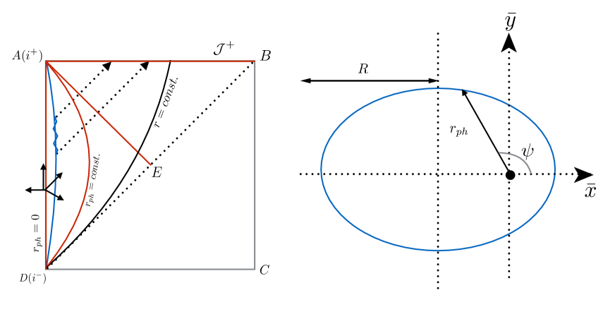
Figure 2: In de Sitter background $r=consant.$ hypersurfaces intersect $\mathcal{J}^{+}$. Red lines denote $r_{ph}:=ar=consant$ surfaces, which are also Killing surfaces. AE denotes the cosmological horizon ($r_{ph}=H^{-1}$) of the source. The spatially compact source is well inside the cosmological horizon. Blue line is the worldline of source trajectory which follows an elliptic orbit in de Sitter background. A tetrad frame is attached to the focus of ellipse.

We will consider a binary system in an elliptic Keplerian orbit. Therefore in the center of mass frame of binary, this system is equivalent to an effective one body problem with reduced mass $\mu=\frac{m_{1}m_{2}}{M}$ following an elliptic trajectory, where $M=m_{1}+m_{2}$ is the total mass of the system. As source moment is defined in tetrad variable, we will attach the tetrad system of conformal chart to the center of mass of the system and assign $r_{ph}=0$ to the focus of ellipse. We also want to express orbital parameters in terms of physical variables. As tetrad component measures physical distance, the orbital parameters should also be expressed in tetrad variable (this automatically incorporates the effect of scale factor in the orbit). In terms of orbital parameters, eccentricity ($\epsilon$) and semi-major axis ($R$), the equation of orbit in de Sitter background is defined by,

$$r_{ph}=\frac{R(1-\epsilon^{2})}{1+\epsilon\cos\psi}$$ (21)

$r_{ph}$ denotes relative physical separation between two components of binary. This definition of the orbit is motivated by the fact that any frame observer of de Sitter background measures the orbital separation as an ellipse.

As discussed earlier, moments should be defined in the tetrad frame. We choose the time direction of tetrad frame along the worldline (measures the proper time $t$) of source and a triad frame $(\bar{x},\bar{y},\bar{z})$ is attached to the focus of the ellipse such that the orbit is restricted to $(\bar{x},\bar{y})$ plane and is given by,

$$\bar{x}(t)=r_{ph}~{}\cos{\psi}~{}~{},~{}~{}~{}\bar{y}(t)=r_{ph}~{}\sin{\psi}~{}~{},~{}~{}~{}\bar{z}(t)=0$$ (22)

Hence, from eq. (12) the mass quadrupole moment of the binary system can be written in a matrix form ,

$${Q}^{ij}=\mu{r_{ph}^{2}}~{}\begin{pmatrix}\cos^{2}\psi&\sin\psi\cos\psi&0\\ \sin\psi\cos\psi&\sin^{2}\psi&0\\ 0&0&0\end{pmatrix}$$ (23)

We restrict our analysis to the adiabatic limit, i.e., the time scale for orbital parameters to change is much longer than orbital time period. For example, this is equivalent to saying $\mid\frac{\Delta E}{E}\mid\ll 1$, where $\Delta{E}$ denotes change in energy of the system over one period and $E$ is the total energy of the system. This can be seen easily from the leading term of eq. (26), $\mid\frac{\Delta E}{E}\mid=\mid\frac{\langle P\rangle T_{P}}{E}\mid\sim\frac{\mu}{M}\big{(}\frac{GM}{R}\big{)}^{5/2}\ll 1$. At this point, it is worthy to mention that to study the secular change in orbital parameters one needs to investigate the change over a period, only instantaneous change does not help. For a circular orbit, instantaneous power does not have angular dependence (see eq. (57)), hence average over one time period is same as the unaveraged answer. But for elliptic orbit instantaneous power has angular dependence, hence averaging plays a crucial role. In adiabatic approximation, the orbital parameters, semi-major axis and eccentricity of elliptic orbit (or equivalently energy and angular momentum) are assumed to be constant of motion over one orbital time period. The system spends many periods near any point of its phase space trajectory. As the gravitational radiation carries both energy and angular momentum, the binary system undergoes secular changes, both in its semi-major axis and eccentricity. For our purpose, in the next section, we concentrate on energy loss and consequent orbital decay rate (time derivative of the period).

V Power radiation from inspiraling binary

At first we would like to compute power radiated by an elliptic inspiraling binary system due to new quadrupole formula in eq. (9). Now using $\Lambda$ projection, $\mathcal{Q}_{ij}^{tt}\mathcal{Q}^{ij}_{tt}:=\Lambda_{~{}ij}^{kl}\mathcal{Q}_{kl}\Lambda^{ij}_{~{}mn}\mathcal{Q}^{mn}=\Lambda^{kl}_{~{}mn}\mathcal{Q}_{kl}\mathcal{Q}^{mn}$, eq. (9) can be written as,

$$\mathcal{P}=\frac{G}{5}\big{\langle}\mathcal{Q}_{ij}\mathcal{Q}^{ij}-\frac{1}{3}\mathcal{Q}^{2}\big{\rangle},$$ (24)

where $\mathcal{Q}:=\delta^{ij}\mathcal{Q}_{ij}$. In deriving this expression we have used the identity for $\Lambda$ projector, $\int d^{2}S~{}\Lambda^{ij}_{~{}kl}=\frac{2\pi}{15}~{}\bigg{[}11\delta^{i}_{k}\delta^{j}_{l}-4\delta^{ij}_{kl}+\delta^{i}_{l}\delta^{j}_{k}\bigg{]}$. For a weakly stressed non-relativistic system, as for Newtonian fluids, pressure can be neglected compared to the energy density, so we can neglect the pressure quadrupole moment terms in eq. (10). Hence neglecting the pressure quadrupole moment terms, power radiated by binary system can be expressed as,

$$\mathcal{P} =\frac{G}{5}\big{\langle}\mathcal{Q}_{ij}\mathcal{Q}^{ij}-\frac{1}{3}\mathcal{Q}^{2}\big{\rangle}$$ (25)

$$\approx\frac{32G^{4}\mu^{2}M^{3}}{5R^{5}}~{}f(\epsilon)+~{}\frac{8H^{2}G^{3}\mu^{2}M^{2}}{R^{2}}~{}g(\epsilon)+~{}\frac{8H^{4}G^{2}\mu^{2}MR}{5}~{}h(\epsilon)$$ (26)

where $f(\epsilon),g(\epsilon),h(\epsilon)$ are

$$f(\epsilon) =(1-\epsilon^{2})^{-7/2}~{}\bigg{(}1+\frac{73}{24}\epsilon^{2}+\frac{37}{96}\epsilon^{4}\bigg{)},$$ (27)

$$g(\epsilon) =(1-\epsilon^{2})^{-1/2}~{}\bigg{[}\frac{4-\sqrt{1-\epsilon^{2}}}{3}\bigg{]},$$ (28)

$$h(\epsilon) =1-\frac{\epsilon^{2}}{3}.$$ (29)

Note that each of these functions approaches unity as $\epsilon\rightarrow 0$. Schematics of the quadrupolar power computation are given in appendix A. Order $H$ and $H^{3}$ terms exactly vanish, after taking time average over orbital period. This can also be understood by the following observation. When direction of time is reversed, orbit goes from anticlockwise to clockwise direction and radiated energy does not depend on the orientation of revolution. The order $H$ and $H^{3}$ terms in (57) have been generated from odd number of time derivatives of moment and thus have odd parity under time reversal and therefore have to vanish. For $\Lambda\rightarrow 0$, this formula reduces to the usual formula for quadrupolar power radiation by the binary system in an elliptic orbit Peters .

To know the order of magnitude, for simplicity let us take a look at power radiated by a circular orbit. Taking $\epsilon\rightarrow 0$ in the eq. (26) we obtain the expression for circular orbit,

$$\mathcal{P}\approx\frac{32G^{4}\mu^{2}M^{3}}{5~{}R^{5}}~{}\bigg{[}1+\frac{5}{4}~{}\frac{H^{2}R^{3}}{GM}+\frac{1}{4}~{}\frac{H^{4}R^{6}}{G^{2}M^{2}}~{}\bigg{]}$$ (30)

This expression has the dimensionless expansion parameter $\frac{H^{2}R^{3}}{GM}$. As mentioned in Satya , a compact binary that coalesces after passing through the last stable orbit is a powerful source of gravitational waves, we assume $R=r_{LSO}=3R_{S}$. Take $m_{1}=m_{2}=1M_{\odot}$ and using Schwarzschild radius of sun, $R_{S}=2GM_{\odot}=3\times 10^{3}meters$,

$$\frac{H^{2}R^{3}}{GM}=\frac{2H^{2}R_{S}^{3}}{R_{S}}\times 27=H^{2}R_{S}^{2}\times 54\approx 10^{-52}\times 10^{6}\times 10^{2}\approx 10^{-44}$$ (31)

It is customary and convenient to express (30) in terms of chirp mass and gravitational wave frequency. For circular orbit substituting $\omega_{s}=\sqrt{\frac{GM}{{R}^{3}}}$. Hence, power loss due to gravitational radiation from a circular binary orbit can be expressed as,

$$\mathcal{P} \approx\frac{32G\mu^{2}R^{4}\omega_{s}^{6}}{5}~{}\bigg{(}1+\frac{5}{4}H^{2}\omega_{s}^{-2}+\frac{1}{4}{H^{4}\omega_{s}^{-4}}\bigg{)}$$

$$=\frac{32}{5G}~{}\bigg{(}\frac{GM_{c}~{}\omega_{gw}}{2}\bigg{)}^{10/3}\bigg{[}1+5H^{2}\omega_{gw}^{-2}+{4}H^{4}\omega_{gw}^{-4}\bigg{]}$$ (32)

where we introduce the chirp mass $M_{c}:={\mu}^{3/5}{M}^{2/5}$ and $\omega_{gw}=2\omega_{s}$. This result matches with that of Bonga (see eq. (25) of the reference). It is also clear from eq. (V) - correction terms are down by $H^{2}/\omega_{gw}^{2}$, e.g., for LIGO (frequency band $f\sim 10^{2}-10^{3}$ Hz), $H^{2}/\omega^{2}_{gw}\sim(\lambdabar/L_{B})^{2}\sim 10^{-42}-10^{-44}$, while for PTA ($f\sim 10^{-6}-10^{-9}$ Hz), the order of magnitude of leading order correction term is $10^{-20}-10^{-26}$. Though the correction terms are more significant for low frequency band detectors, they are still negligible.

VI angular momentum radiation

It is well known that Isaacson stress-energy tensor does not suffice to capture flux of angular momentum even in Minkowski background Gravity . Nevertheless, one can employ the formalism of covariant phase space to get a correct expression for angular momentum flux. We use the formalism developed in ABKIII to compute angular momentum flux radiated by a binary system in de Sitter background. The instantaneous angular momentum radiation in de Sitter background is given byABKIII ,

$$\dot{L}_{k}=\frac{G}{4\pi}\ \epsilon_{ik}\ ^{m}\int d^{2}S\big{(}\mathcal{Q}^{ij}\big{)}\big{(}\mathcal{L}_{T}^{2}Q_{jm}+H\mathcal{L}_{T}Q_{jm}+H\mathcal{L}_{T}\bar{Q}_{jm}+H^{2}\bar{Q}_{jm}\big{)}^{TT}$$ (33)

Average angular momentum radiated by an elliptic binary over a orbital time period is given by after performing an $S^{2}$ integral,

$$\big{\langle}\dot{L}_{k}\big{\rangle}=\frac{2G}{5}\epsilon_{ik}\ ^{m}\Big{\langle}\big{(}\mathcal{Q}^{ij}\big{)}\big{(}\mathcal{L}_{T}^{2}Q_{jm}+H\mathcal{L}_{T}Q_{jm}+H\mathcal{L}_{T}\bar{Q}_{jm}+H^{2}\bar{Q}_{jm}\big{)}\Big{\rangle},$$ (34)

where in deriving this expression we have used local projector to extract the TT part. Neglecting the pressure quadrupole moments, the expression for angular momentum radiation can be found in the same manner as energy radiation. As the binary system is restricted in $x-y$ plane, the $z$ component of emitted angular momentum flux (over an orbital period) is given by,

$$\big{\langle}\dot{L}_{z}\big{\rangle} =\frac{2G}{5}\epsilon_{iz}\ ^{m}\Big{\langle}\big{(}\mathcal{Q}^{ij}\big{)}\big{(}\mathcal{L}_{T}^{2}Q_{jm}+H\mathcal{L}_{T}Q_{jm}+H\mathcal{L}_{T}\bar{Q}_{jm}+H^{2}\bar{Q}_{jm}\big{)}\Big{\rangle}$$ (35)

$$\approx\frac{32G^{7/2}\mu^{2}M^{5/2}}{5R^{7/2}}~{}F(\epsilon)+~{}\frac{8H^{2}G^{5/2}\mu^{2}M^{3/2}}{R^{1/2}}~{}G(\epsilon)+~{}\frac{8H^{4}G^{3/2}\mu^{2}M^{1/2}R^{5/2}}{5}~{}H(\epsilon)$$ (36)

where $F(\epsilon),G(\epsilon),H(\epsilon)$ are

$$F(\epsilon) =\frac{1}{(1-\epsilon^{2})^{2}}~{}\big{(}1+\frac{7}{8}\epsilon^{2}\big{)},$$ (37)

$$G(\epsilon) =(1-\epsilon^{2})^{1/2},$$ (38)

$$H(\epsilon) =(1-\epsilon^{2})^{1/2}(1+\frac{3}{2}\epsilon^{2}).$$ (39)

It should be noted that each of these functions approaches unity as $\epsilon\rightarrow 0$. Further details of the above computation are given in appendix A. Here also order $H$ and $H^{3}$ do not contribute. For $t\rightarrow-t$, the direction of angular momentum gets flipped. The order $H$ and $H^{3}$ terms in angular momentum flux computation have been generated from even number of time derivatives of moment and thus have even parity under time reversal and therefore have to vanish. From eq. (26) and (36) it is evident that for circular case $\langle\dot{E}\rangle=\omega_{s}\langle\dot{L}_{z}\rangle$.

VII evolution of orbital parameters

The results of previous two sections can be applied to compute secular change in orbital parameters. A priori it is not clear whether the conservative dynamics of binary is governed by Newtonian Potential. We assume that near the source the space-time geometry is Schwarzschild de Sitter. In the weak field limit around flat background repulsive nature of de Sitter potential comes into play and correction terms generated by this potential is also of same order $\frac{H^{2}r_{ph}^{3}}{GM}$ (it is clear from eq. (80) in appendix B). But we are analyzing perturbation around de Sitter background and we relate field solution in terms of source moments using conservation equation on de Sitter background. Therefore, it is necessary to investigate weak field limit on pure de Sitter background. A full resolution of this problem requires expansion over Schwarzschild de Sitter metric using the technique of black hole perturbation theory which is beyond the scope of this work. In appendix B, we have argued that in the weak field limit on de Sitter background the potential can be still be assumed to be Newtonian. The repulsive nature of de Sitter potential can be absorbed in background itself. Hence the orbital parameters $R,\epsilon$ are related to $E$ and $L$ through following equations,

$$R=-\frac{GM\mu}{2E},$$ (40)

$$\epsilon^{2}=1+\frac{2EL^{2}}{G^{2}M^{2}\mu^{3}}$$ (41)

Using equations (26), (36) we obtain $\langle\dot{R}\rangle$ and $\langle\dot{\epsilon}\rangle$,

$$\langle{\dot{R}}\rangle = -\bigg{(}\frac{64}{5}\frac{G^{3}\mu M^{2}}{R^{3}}f(\epsilon)+16H^{2}G^{2}\mu Mg(\epsilon)+\frac{16}{5}H^{4}G\mu R^{3}h(\epsilon)\bigg{)}$$ (42)

$$\langle\dot{\epsilon}\rangle= - \frac{304}{15}\frac{G^{3}\mu M^{2}}{R^{4}}\frac{\epsilon}{(1-\epsilon^{2})^{5/2}}\Big{(}1+\frac{121}{304}\epsilon^{2}\Big{)}$$ (43)

$$- \frac{32}{3}\frac{H^{2}G^{2}\mu M}{R}\frac{(1-\epsilon^{2})^{1/2}}{\epsilon}\big{(}1-\sqrt{1-\epsilon^{2}}\big{)}+\frac{44}{15}H^{4}G\mu R^{2}\epsilon(1-\epsilon^{2})$$

For $H\rightarrow 0$, these results match with usual flat space results. From eq. (43) we see that for $\epsilon\rightarrow 0$, $\langle\dot{\epsilon}\rangle=0$. Therefore, circular orbit remains circular. It should also be noted that the contribution from $H^{4}$ term is positive but the smallness of $H^{2}R^{3}/GM$ ensures that $H^{2}$ term dominates making the overall contribution negative. For an elliptic orbit $0<\epsilon<1$, eq. (43) gives $\langle\dot{\epsilon}\rangle<0$. Therefore, elliptic orbit becomes more and more circular due to emission of gravitational waves. To get the time to coalescence for circular orbit one needs to integrate eq. (42). We do not give the full expression to avoid the cluttering, in this case also leading order correction term is of the order $H^{2}R^{3}/GM$.

Now, let us investigate an observable parameter $\dot{P_{b}}$ (time derivative of orbital period) for elliptic orbit. Orbital period $P_{b}$ is related to orbital energy as $P_{b}=constant\times(-E)^{3/2}$. Hence,

$$\frac{\dot{P}_{b}}{P_{b}} =-\frac{3}{2}~{}\frac{\dot{E}}{E}$$ (44)

Assuming that the binary system is loosing energy entirely due to quadrupolar radiation, substituting eq. (26) in $\dot{E}$, we find

$${\dot{P}_{b}}=-\frac{192\pi}{5}~{}{G^{5/3}\mu M^{2/3}}~{}\bigg{(}\frac{P_{b}}{2\pi}\bigg{)}^{-5/3}f(\epsilon)\times\bigg{[}1+{\frac{5}{4}}H^{2}\bigg{(}\frac{P_{b}}{2\pi}\bigg{)}^{2}~{}\frac{g(\epsilon)}{f(\epsilon)}+{\frac{1}{4}}H^{4}\bigg{(}\frac{P_{b}}{2\pi}\bigg{)}^{4}~{}\frac{h(\epsilon)}{f(\epsilon)}\bigg{]},$$ (45)

where the average over an orbital period is understood. In the intermediate step we have also used $E=-\frac{G\mu M}{2R}$ and $P_{b}=2\pi\sqrt{\frac{R^{3}}{GM}}$. For Hulse-Taylor Pulsar the values of relevant parameters are: $m_{1}=1.4414M_{\odot},m_{2}=1.3867M_{\odot},\epsilon=0.617338,P_{b}=2.790698\times 10^{4}s$ Satya . Hence, for Hulse-Taylor binary first order correction for orbital decay rate,

$$\frac{5}{4}H^{2}\bigg{(}\frac{P_{b}}{2\pi}\bigg{)}^{2}~{}\frac{g(\epsilon)}{f(\epsilon)}=\frac{5}{4}\times\frac{10^{-35}}{3}\times\bigg{(}\frac{P_{b}}{2\pi}\bigg{)}^{2}~{}\frac{g(\epsilon)}{f(\epsilon)}\sim 10^{-29}$$ (46)

Current accuracy level of the observation of orbital decay rate of Hulse-Taylor pulsar is at $10^{-3}$. Hence correction terms due to $\Lambda$ are utterly negligible in the current observational context.

VIII Comparision between TT vs tt

In this section, we compare our result with that of obtained in a recent paper Bonga . The procedure to obtain power emitted by elliptic orbit in our work is completely different from the ref. Bonga . In our paper we use local algebraic tt projector to obtain the power radiation while ref. Bonga relies on extracting transverse traceless (TT) part of source quqdrupole moment. For clarity, let us recall that any symmetric rank-2 tensor field can be decomposed as Gravity ,

$$Q_{ij}=\frac{1}{3}\delta_{ij}\delta^{kl}Q_{kl}+(\partial_{i}\partial_{j}-\frac{1}{3}\delta_{ij}\nabla^{2})B+\partial_{i}B_{j}^{T}+\partial_{j}B_{i}^{T}+Q_{ij}^{TT}.$$

$Q_{ij}^{TT}$ refers to the transverse-traceless part of the field, so that $\partial^{i}Q_{ij}^{TT}=0=\delta^{ij}Q_{ij}^{TT}$. Algebraically projected tt fields are is defined as $Q_{ij}^{tt}:=\Lambda_{ij}^{kl}Q_{kl}$, with $\Lambda_{ij}^{kl}:=\frac{1}{2}(P_{i}^{k}P_{j}^{l}+P_{i}^{l}P_{j}^{k}-P_{ij}P^{kl})\ \mbox{and}~{}P_{i}^{j}=\delta_{i}^{j}-\hat{x}_{i}\hat{x}^{j}$. $\Lambda$ projected tensor fields satisfy spatial transversality and tracelessness (TT) condition to the leading order in $r^{-1}$ DateJH2 . For a detailed analysis between tt vs. TT in the context of asymptotically flat space-time, see ABI ; ABII . A priori these two notions are distinct and inequivalent. Although these two notions match at future null infinity for Minkowski space-time, they are quite different in de Sitter space-time. The tt-projection is well tailored to the $1/r$ expansion commonly used for asymptotically flat spacetimes. As the global structure of de Sitter spacetime is different from Minkowski spacetime, expansion in powers of $1/r$ is not a useful tool to analyse asymptotically de Sitter spacetimes. In particular, the tt-projection is not a valid operation to extract the transverse-traceless part of a rank-2 tensor on the full $\mathcal{J}^{+}$. The TT-tensor is the correct notion of transverse traceless tensors. However, if one restricts oneself to large radial distances away from the source, one may expect that the tt-projection also gives useful answers. We stick to tt projection throughout our paper and emphasize that in the context of power radiated by a circular binary system in de Sitter background the answer exactly matches with that of computation done in ref Bonga using TT (see eq. (25) of the reference). Though explicit expression of $Q_{ij}^{TT}$ and $Q_{ij}^{tt}$ are quite different (see eq. (20) of ref. Bonga ) even in $\mathcal{J}^{+}$ of de Sitter space-time, after integration over two-sphere in energy flux formula the resulting expression for power is the same. This observation is new and indicates that for energy flux computation by a circular binary, TT vs tt does not matter in de Sitter background. We also compare our angular momentum flux expression to the leading order expression obtained in Bonga (see eq. (26) of the reference) for circular orbit. To the leading order in $H^{0}$ it matches exactly. We expect the higher order correction terms in $H$ will also match as the tt operation generates an overall factor.

IX summary and discussion

In this short paper, we obtain quadrupolar energy and angular momentum loss due to gravitational radiation for a generic elliptic binary system in de Sitter background. We also discuss the decay of eccentricity and semi-major axis due to gravitational radiation. As noted earlier, the modified quadrupole formula can impact both direct and indirect observations of gravitational waves. While indirect observations track orbital decay rate of the binary system, direct observation in gravitational wave astronomy is sensitive to changes in the orbital phase. This paper focuses on the former and concludes that impact of $\Lambda$ in orbital decay is negligible in the context of current accuracy of observations. From dimensional analysis one may argue that correction terms due to $\Lambda$ should be $\sqrt{\Lambda}\times lengthscale$. This correction may be relevant over cosmological distances, e.g. mega-parsec. There are two natural length scales - one is observational distance and another is source dimension. It should be noted that though linearized field expression depends on observational length scale, energy and angular momentum flux are independent of observational length scale. Hence, only available length scale is orbital length scale which enters into the expression via the definition of source quadrupole moments. A typical compact object has orbital extension to the order of $10^{6}~{}m$. Hence, this crude analysis also suggests that the correction terms should be of the order of $\sqrt{\Lambda}\times orbital~{}lengthscale\sim 10^{-26}\times 10^{6}=10^{-20}$. In our case, the correction terms are even smaller as order $H(\sqrt{\Lambda/3})$ term drops out and leading correction term is of the order $H^{2}$.

In this paper we also emphasize that for power radiated by a circular binary in de Sitter background, identification of TT vs tt does not matter. Why these two completely distinct notions give the same answer for energy flux of circular orbit in de Sitter space-time is still needed to be understood clearly. Whether this result generalizes to ellipitic orbit case or for other sources is still needed to be investigated.

Appendix A Energy and angular momentum radiated by an elliptic binary

As computation of radiated energy and angular momentum need derivative of moments, let us give the expressions for derivative of moments. Taking the quadrupolar mass moment tensor (23) for elliptic orbit, derivatives of different components are given by,

$$\dot{Q}_{11} =\dfrac{-\alpha}{1+\epsilon\cos\psi}\sin{2\psi},$$ (47)

$$\dot{Q}_{12} =\dfrac{\alpha}{1+\epsilon\cos\psi}(\epsilon\cos\psi+\cos{2\psi}),$$ (48)

$$\dot{Q}_{22} =\dfrac{2\alpha}{1+\epsilon\cos\psi}(\epsilon\sin{\psi}+\sin{\psi}\cos{\psi}),~{}~{}~{}~{}~{}~{}~{}~{}~{}~{}~{}~{}~{}~{}~{}~{}\mbox{ with $\alpha=\mu\sqrt{GMR(1-\epsilon^{2})}.$}$$ (49)

$$\ddot{Q}_{11} =-\beta[2\cos{2\psi}(1+\epsilon\cos\psi)+e\sin{2\psi}\sin\psi)],$$ (50)

$$\ddot{Q}_{12} =-2\beta[\sin{2\psi}+\epsilon\sin{\psi}(1+\cos^{2}\psi)],$$ (51)

$$\ddot{Q}_{22} =2\beta[\cos{2\psi}+\epsilon\cos{\psi}(1+\cos^{2}\psi)+\epsilon^{2}],~{}~{}~{}~{}~{}~{}~{}~{}~{}~{}~{}~{}~{}~{}~{}~{}~{}~{}~{}~{}~{}~{}~{}~{}~{}\mbox{ with $\beta=\frac{\mu GM}{R(1-\epsilon^{2})}.$}$$ (52)

$$\dddot{Q}_{11} =\gamma(1+\epsilon\cos\psi)^{2}[2\sin{2\psi}+3\epsilon\,\sin\psi\,\cos^{2}\psi],$$ (53)

$$\dddot{Q}_{12} =\gamma(1+\epsilon\cos\psi)^{2}[-2\cos{2\psi}+\epsilon\cos\psi(1-3\cos^{2}\psi)],$$ (54)

$$\dddot{Q}_{22} =-\gamma(1+\epsilon\cos\psi)^{2}[2\sin{2\psi}+\epsilon\sin\psi(1+3\cos^{2}\psi)],~{}~{}~{}~{}~{}~{}\mbox{ with $\gamma=\frac{2\mu(GM)^{3/2}}{R^{5/2}(1-\epsilon^{2})^{5/2}}.$}$$ (55)

The expression for radiated power is given by (24),

$$\mathcal{P}=\frac{G}{5}\big{\langle}\mathcal{Q}_{ij}\mathcal{Q}_{ij}-\frac{1}{3}\mathcal{Q}^{2}\big{\rangle}:=\langle P(\psi)\rangle$$ (56)

Now we plug the derivatives of moments in computing unaveraged quantity $P(\psi)$ and express our result order by order in $H$.

$$P(\psi)\approx \frac{8G^{4}}{15}~{}\frac{\mu^{2}M^{3}}{R^{5}(1-\epsilon^{2})^{5}}(1+\epsilon\cos{\psi})^{4}~{}\big{[}12(1+\epsilon\cos{\psi})^{2}+\epsilon^{2}\sin^{2}{\psi}\big{]}$$ (57)

$$+ \frac{4G^{7/2}H}{5}~{}\frac{\epsilon~{}\mu^{2}M^{5/2}}{R^{7/2}(1-\epsilon^{2})^{7/2}}~{}\sin{\psi}(1+\epsilon\cos{\psi})^{2}~{}[18+13\epsilon^{2}+40\epsilon\cos{\psi}+9\epsilon^{2}\cos{2\psi}]$$

$$+ \frac{2G^{3}H^{2}}{15}~{}\frac{\mu^{2}M^{2}}{(1-\epsilon^{2})^{2}~{}R^{2}}~{}\big{[}60+100\epsilon^{2}+36\epsilon^{4}+\epsilon(180+113\epsilon^{2})\cos\psi+116\epsilon^{2}\cos 2\psi+19\epsilon^{3}\cos 3\psi\big{]}$$

$$- \frac{32G^{5/2}H^{3}}{5}~{}\frac{\epsilon^{2}\mu^{2}M^{3/2}}{\sqrt{R(1-\epsilon^{2})}}~{}\frac{\sin\psi(\epsilon+\cos\psi)}{1+\epsilon\cos\psi}$$

$$+ \frac{4G^{2}H^{4}}{15}~{}\frac{\mu^{2}MR(1-\epsilon^{2})}{(1+\epsilon\cos\psi)^{2}}~{}\big{[}6+7\epsilon^{2}+12\epsilon\cos\psi{-}\epsilon^{2}\cos 2\psi\big{]}$$

In the intermediate step we have neglected pressure quadrupole moment term in eq. (10) and used $\mathcal{Q}_{ij}\approx\partial_{t}^{3}Q_{ij}-3H\partial_{t}^{2}Q_{ij}+2H^{2}\partial_{t}Q_{ij}$. To get the expression for power we have to perform an averaging integral of (57). An explicit averaging procedure is illustrated in the appendix of DateJH2 . It permits to split four-dimensional averaging integral into an integral over $r_{ph}=constant$ hypersurface and a three dimensional flux integral. The averaging integral over $r_{ph}=constant$ hypersurface and angular integral can be done explicitly, leaving the four-dimensional averaging integral to a time-averaged quantity only. Hence average power over an orbital period is given by

$$\mathcal{P}= \frac{1}{T}\int_{0}^{T}dtP(\psi)=\frac{\omega_{s}}{2\pi}\int_{0}^{2\pi}\frac{d\psi}{\dot{\psi}}P(\psi)$$ (58)

$$= \bigg{(}\frac{GM}{R^{3}}\bigg{)}^{1/2}\times\frac{1}{2\pi}\int_{0}^{2\pi}\frac{d\psi}{\dot{\psi}}P(\psi)$$ (59)

Using 57 we obtain,

$$\mathcal{P}=\frac{32G^{4}\mu^{2}M^{3}}{5R^{5}}~{}f(\epsilon)+~{}\frac{8H^{2}G^{3}\mu^{2}M^{2}}{R^{2}}~{}g(\epsilon)+~{}\frac{8{H^{4}G^{2}\mu^{2}MR}}{5}~{}h(\epsilon)$$ (60)

where,

$$f(\epsilon) =(1-\epsilon^{2})^{-7/2}~{}\bigg{(}1+\frac{73}{24}\epsilon^{2}+\frac{37}{96}\epsilon^{4}\bigg{)},$$ (61)

$$g(\epsilon) =(1-\epsilon^{2})^{-1/2}~{}\bigg{[}\frac{4-\sqrt{1-\epsilon^{2}}}{3}\bigg{]},$$ (62)

$$h(\epsilon) =1-\frac{\epsilon^{2}}{3}.$$ (63)

Deriving this expression we have used $\dot{\psi}=\frac{\sqrt{GMR(1-\epsilon^{2})}}{r_{ph}^{2}}$ for elliptic Keplerian orbit.
      We follow the same procedure for angular momentum flux. Neglecting pressure quadrupole moments and writing $\mathcal{L}_{T}$ in terms of $\partial_{t}$ the equation (34) becomes,

$$\Big{\langle}\dot{L}_{z}\Big{\rangle}\approx\frac{2G}{5}\ \epsilon_{iz}\ ^{m}\Big{\langle}\big{(}\partial_{t}^{3}Q_{ij}-3H\partial_{t}^{2}Q_{ij}+2H^{2}\partial_{t}Q_{ij}\big{)}\big{(}\partial_{t}^{2}Q_{ij}-3H\partial_{t}Q_{ij}+2H^{2}Q_{ij}\big{)}\Big{\rangle}$$ (64)

Plugging the derivatives of moments, the unaveraged quantity becomes,

$$\dot{L}_{z}\approx \frac{4G^{7/2}}{5}~{}\frac{\mu^{2}M^{5/2}}{R^{7/2}(1-\epsilon^{2})^{7/2}}(1+\epsilon\cos{\psi})^{3}~{}\big{[}8+\epsilon^{2}+12\epsilon\cos\psi+3\epsilon^{2}\cos 2\psi\big{]}$$ (65)

$$+ \frac{36G^{3}H}{5}~{}\frac{\epsilon~{}\mu^{2}M^{2}}{R^{2}(1-\epsilon^{2})^{2}}~{}\sin{\psi}(1+\epsilon\cos{\psi})^{2}~{}$$

$$+ \frac{4G^{5/2}H^{2}}{5}~{}\frac{\mu^{2}M^{3/2}}{(1-\epsilon^{2})^{1/2}~{}R^{1/2}}~{}\big{[}10+7\epsilon^{2}+17\epsilon\cos\psi\big{]}$$

$$- \frac{24G^{2}H^{3}}{5}~{}\frac{\epsilon\mu^{2}MR\sin\psi}{1+\epsilon\cos\psi}+\frac{8G^{3/2}H^{4}}{5}~{}\frac{\mu^{2}M^{1/2}R^{5/2}(1-\epsilon^{2})^{5/2}}{(1+\epsilon\cos\psi)^{2}}~{}$$

Therefore, average angular momentum radiation over an orbital time period is given by,

$$\Big{\langle}\dot{L}_{z}\Big{\rangle} =\frac{1}{T}\int_{0}^{T}d\tau~{}\frac{dL_{z}}{d\tau}$$ (66)

$$\approx\frac{32G^{7/2}\mu^{2}M^{5/2}}{5R^{7/2}}~{}F(\epsilon)+~{}\frac{8H^{2}G^{5/2}\mu^{2}M^{3/2}}{R^{1/2}}~{}G(\epsilon)+~{}\frac{8H^{4}G^{3/2}\mu^{2}M^{1/2}R^{5/2}}{5}~{}H(\epsilon)$$ (67)

where $F(\epsilon),G(\epsilon),H(\epsilon)$ are

$$F(\epsilon) =\frac{1}{(1-\epsilon^{2})^{2}}~{}\big{(}1+\frac{7}{8}\epsilon^{2}\big{)},$$ (68)

$$G(\epsilon) =(1-\epsilon^{2})^{1/2},$$ (69)

$$H(\epsilon) =(1-\epsilon^{2})^{1/2}(1+\frac{3}{2}\epsilon^{2}).$$ (70)

Appendix B Weak field limit on de Sitter background

We follow the same procedure of Minkowski background to extract the effective potential in de Sitter background. The equation for geodesic is given by,

$$\frac{d^{2}x^{\mu}}{d\tau^{2}}+\Gamma^{\mu}_{\nu\rho}\frac{dx^{\nu}}{d\tau}\frac{dx^{\rho}}{d\tau}=0$$ (71)

For our case the background de Sitter metric is given by,

$$\bar{ds}^{2}=-dt^{2}+e^{2Ht}dx^{i}dx^{j}\delta_{ij}$$ (72)

Hence, proper time $\tau$ is given by $t$ and for non-relativistic case, we can neglect $dx^{i}/dt$ terms. Hence the geodesic equation becomes,

$$\frac{d^{2}x^{i}}{dt^{2}}+\Gamma^{i}_{00}=0$$ (73)

Now decomposing the metric $g_{\mu\nu}=\bar{g}_{\mu\nu}+h_{\mu\nu}$, to the leading order in $h$, $\Gamma^{i}_{00}$ can be expressed as,

$$\Gamma^{i}_{00}=\bar{\Gamma}^{i}_{00}+\frac{1}{2}\bar{g}^{i\alpha}(2\bar{\nabla}_{0}h_{\alpha 0}-\bar{\nabla}_{\alpha}h_{00})$$ (74)

For background metric the only non-zero components of christoffel-connection are $\bar{\Gamma}^{t}_{ij}=He^{2Ht}\delta_{ij}$ and $\bar{\Gamma}^{i}_{tj}=H\delta^{i}_{j}$. Therefore,

$$2\bar{\nabla}_{0}h_{j0}-\bar{\nabla}_{j}h_{00}=\partial_{0}h_{j0}-\partial_{j}h_{00}$$ (75)

Since we are considering non-relativistic source, the time derivative of metric is of higher order with respect to spatial derivatives ($\frac{\partial}{\partial t}=\mathcal{O}(v)\frac{\partial}{\partial x}$), so to the leading order eqn. (73) becomes,

$$\frac{d^{2}x^{i}}{dt^{2}}=\frac{1}{2}\bar{g}^{ij}\partial_{j}h_{00}\implies A^{i}=\frac{1}{2}e^{-2Ht}\delta^{ij}\partial_{j}h_{00}$$ (76)

As the orbital parameters are described in tetrad frame, we would like to recast this expression in that frame. For the background metric (72), tetrad frame becomes , $f^{\alpha}_{\underline{0}}=\delta^{\alpha}_{0},f^{\alpha}_{\underline{i}}=e^{-Ht}\delta^{\alpha}_{\underline{i}}$. Therefore $A^{i}=e^{-Ht}\bar{A}^{i}$ and $\frac{\partial}{\partial x^{j}}=e^{Ht}\frac{\partial}{\partial\bar{x}^{j}}$ Therefore in this frame geodesic equation becomes,

$$\bar{A}^{i}=\frac{1}{2}\delta^{ij}\frac{\partial h_{00}}{\partial\bar{x}^{j}}$$ (77)

Comparing this equation with Newtonian equation of motion, the term $-\frac{1}{2}h_{00}$ can be thought of as Newtonian potential. Under the coordinate transformations,

$$dt=d\tau-\frac{Hr_{ph}}{1-H^{2}r_{ph}^{2}}dr_{ph}~{},~{}~{}r=e^{-Ht}r_{ph}$$ (78)

background metric (72) becomes,

$$\bar{ds}^{2}=-(1-H^{2}r_{ph}^{2})d\tau^{2}+\frac{dr_{ph}^{2}}{(1-H^{2}r_{ph}^{2})}+r_{ph}^{2}(d\theta^{2}+\sin^{2}\theta d\phi^{2})$$ (79)

It should be noted that tetrad frame measure physical distance, $r_{ph}$ and time direction is taken along worldline of centre of mass (for which $r_{ph}=0$). Therefore $dt=d\tau$ in this frame. Now in Schwarschild de Sitter geometry the metric takes the form,

$$ds^{2}=-(1-H^{2}r_{ph}^{2}-\frac{2Gm}{r_{ph}})d\tau^{2}+\frac{dr_{ph}^{2}}{(1-H^{2}r_{ph}^{2}-\frac{2Gm}{r_{ph}})}+r_{ph}^{2}(d\theta^{2}+\sin^{2}\theta d\phi^{2})$$ (80)

Therefore, on pure de Sitter background the motion is still governed by Newtonian potential in weak field limit.

References

• (1) A. Einstein, ̈Uber Gravitationswellen, Sitzungsberichte der Königlich Preußischen Akademie der Wissenschaften (Berlin), 154-167 (1918).
• (2) R.A. Hulse and J.H. Taylor, Discovery of a pulsar in a binary system, Astrophys. J., 195, L51-L53 (1975).
• (3) J.H. Taylor and J. M. Weisberg, A new test of general relativity : Gravitational radiation and the binary PSR 1913+1916, Astrophys. J., 253, 908-920 (1982).
• (4) T. Damour, 1974 : The discovery of the first binary pulsar, Class. Quant. Grav., 32, 124009 (2015).
• (5) B. P. Abbott et al., Observation of Gravitational Waves from a Binary Black Hole Merger, Phys. Rev. Lett., 116, 061102 (2016).
• (6) B. P. Abbott et al., GW151226: Observation of Gravitational Waves from a 22- Solar-Mass Binary Black Hole Coalescence, Phys. Rev. Lett., 116, 241103 (2016).
• (7) B. P. Abbott et al., GW170104: Observation of a 50-Solar-Mass Binary Black Hole Coalescence at Redshift 0.2, Phys. Rev. Lett., 118, 221101 (2017).
• (8) B. P. Abott et al., GW170814 : A three-detector observation of gravitational waves from a binary black hole coalescence, [arXiv:1709.09660].
• (9) A. Aggarwal, Estimating the effects of a small positive $\Lambda$ in orbital decay of binaries, Master’s thesis, June 2017.
• (10) S. J. Hoque, Physics of Gravitational Waves in Presence of Positive Cosmological Constant, PhD thesis, June 2017.
• (11) R. A. Isaacson, Gravitational radiation in the limit of high frequency I: The linear approximation and geometrical optics, Phys. Rev., 166, 1263, (1968); R. A. Isaacson, Gravitational radiation in the limit of high frequency II: Non-linear terms and the effective stress tensor, Phys. Rev., 166, 1272, (1968).
• (12) G. Date and S. J. Hoque, Cosmological Horizon and the Quadrupole Formula in de Sitter Background, Phys. Rev. D, 96, 044026 (2017).
• (13) G. Date and S. J. Hoque, Gravitational Waves from Compact Sources in de Sitter Background, Phys. Rev. D, 94, 064039 (2016).
• (14) A. Ashtekar, B. Bonga and A. Kesavan, Asymptotics with a positive cosmological constant: II. Linear fields on de Sitter space-time, Phys. Rev. D, 92, 044011, (2015), [arXiv:1506.06152].
• (15) A. Ashtekar, B. Bonga and A. Kesavan, Asymptotics with a positive cosmological constant: III. The quadrupole formula, Phys. Rev. D, 92, 10432 (2015), [arXiv:1510.05593] .
• (16) S. J. Hoque, A. Virmani, On Propagation of Energy Flux in de Sitter Spacetime, Gen. Rel. Grav. , 50, 4, 40 (2018), [arXiv: 1801.05640].
• (17) Charles W. Misner, Kip S. Thorne, and John Archibald Wheeler, Gravitation, Macmillan, (1973).
• (18) Leo C. Stein and N. Yunes, Effective Gravitational Wave Stress-energy Tensor in Alternative Theories of Gravity, Phys. Rev. D, 83, 064038, (2011), [arXiv: 1012.3144].
• (19) E. Poisson and C.M.Will, Gravity : Newtonian, Post-Newtonian, Relativistic, CUP, 2014.
• (20) E.Poisson, A.Pound and l. Vega, The motion of point particles in curved space- time, Living Rev. Relativity, 14, 7, (2011), [arXiv:1102.0529].
• (21) N. Straumann, General Relativity with Applications to Astrophysics , Springer, Berlin, 2004.
• (22) M. Maggiore, Gravitational waves, Vol 1: Theory and experiments, OUP, 2007.
• (23) A. Bounanno, Gravitational waves, [arXiv: 0709.4682].
• (24) P.C. Peters, J. Mathews, Gravitational radiation from point masses in a Keplerian orbit , Phys. Rev. , 131, 435-440 (1963).
• (25) B.S. Sathyaprakash, B.F. Schutz, Physics, Astrophysics and Cosmology with Gravitational Waves, Living Rev. Relativity, 12, (2009), [arXiv: 0903.0338].
• (26) B. Bonga, J. S. Hazboun, Power radiated by a binary system in a de Sitter Universe, Phys. Rev. D, 96, 064018, (2017), [arXiv:1708.05621].
• (27) A. Ashtekar, B. Bonga, On a basic conceptual confusion in gravitational radiation theory, Class. Quantum Grav., 34, 20LT01, (2017), [arXiv:1707.07729].
• (28) A. Ashtekar, B. Bonga, On the ambiguity in the notion of transverse traceless modes of gravitational waves, Gen. Rel. Gravit., 49, 122, (2017), [arXiv:1707.09914].