MAGNETIC BRAKING OF SUN-LIKE AND LOW-MASS STARS: DEPENDENCE ON CORONAL TEMPERATURE.

Abstract

Sun-like and low-mass stars possess high temperature coronae and lose mass in the form of stellar winds, driven by thermal pressure and complex magnetohydrodynamic processes. These magnetized outflows probably do not significantly affect the star’s structural evolution on the Main Sequence, but they brake the stellar rotation by removing angular momentum, a mechanism known as magnetic braking. Previous studies have shown how the braking torque depends on magnetic field strength and geometry, stellar mass and radius, mass-loss rate, and the rotation rate of the star, assuming a fixed coronal temperature. For this study we explore how different coronal temperatures can influence the stellar torque. We employ 2.5D, axisymmetric, magnetohydrodynamic simulations, computed with the PLUTO code, to obtain steady-state wind solutions from rotating stars with dipolar magnetic fields. Our parameter study includes 30 simulations with variations in coronal temperature and surface-magnetic-field strength. We consider a Parker-like (i.e. thermal-pressure-driven) wind, and therefore coronal temperature is the key parameter determining the velocity and acceleration profile of the flow. Since the mass loss rates for these types of stars are not well constrained, we determine how torque scales for a vast range of stellar mass loss rates. Hotter winds lead to a faster acceleration, and we show that (for a given magnetic field strength and mass-loss rate) a hotter outflow leads to a weaker torque on the star. We derive new predictive torque formulae for each temperature, which quantifies this effect over a range of possible wind acceleration profiles.

1. Introduction

Stellar winds are a very common phenomenon in our universe. For Sun-like and low-mass stars ($M_{*}\lesssim 1.3M_{\odot}$), such outflows are usually in the form of coronal winds (Parker, 1958, 1963), due to their origin in the several MK stellar hot coronae. Although the effect of coronal winds on stellar mass during a star’s Main-Sequence (MS) life is relatively small, they can influence the environment of surrounding planets (e.g. Lüftinger et al., 2015), and have an enormous impact on stellar rotation by exerting a spin-down torque on the stellar surface (e.g. Schatzman, 1962; Weber & Davis, 1967). Hence, over the years the angular momentum (or rotational) evolution of cool stars has been the subject of very intensive studies (for a review see Bouvier et al., 2014).

The spin-down of MS cool stars was established observationally from early studies (Kraft, 1967; Skumanich, 1972) that showed the rotation periods of these types of stars to increase as the stellar age advances. The current picture of the rotational evolution of cool stars is more complicated, and observations (e.g. Barnes, 2003, 2010; Irwin & Bouvier, 2009; Meibom et al., 2011, 2015) show that stellar rotation depends on both the mass and age. In addition, the observed trends between magnetic activity (or coronal X-ray emission) and stellar rotation (e.g. Pizzolato et al., 2003; Wright et al., 2011), and the observed evolution of stellar magnetic properties (e.g. Vidotto et al., 2014b; See et al., 2015) suggest that solar- and late-type stars lose mass and angular momentum in the form of magnetized outflows.

Coronal-wind modeling has a long history in the literature, with the use of analytic theory (e.g. Parker, 1958; Weber & Davis, 1967; Mestel, 1968; Heinemann & Olbert, 1978; Low & Tsinganos, 1986), or iterative methods/numerical simulations (e.g. Pneuman & Kopp, 1971; Sakurai, 1985; Washimi & Shibata, 1993; Keppens & Goedbloed, 2000; Cohen et al., 2007; Vidotto et al., 2009). The main source for understanding the nature, the properties and the dynamics of coronal winds comes from direct observations of the solar wind. The solar corona expands into the interplanetary space in the form of a supersonic, magnetized wind that evolves during a solar cycle. Near the solar minimum the solar wind is bimodal with a fast, tenuous, and steady, component emanating from large polar coronal holes and a slower, denser and filamentary component emerging from the top of the helmet streamers originated at the magnetic activity belt (e.g. McComas et al., 2007, 2008). During the solar maximum the solar wind becomes more variable and is more dominated by the slow wind at all latidtudes (e.g. McComas et al., 2003, 2007). The solar wind is a direct consequence of the hot solar corona (with $T>10^{6}K$) and thus the solar-plasma acceleration (for both the fast and slow solar wind) is connected to the coronal heating problem (e.g. De Moortel & Browning, 2015). The physical mechanisms responsible for the solar-corona heating are still in debate, but they all require magnetic fields as a key ingredient (see, e.g. Aschwanden, 2005; Klimchuk, 2015; Velli et al., 2015). The solar magnetic field (a product of the solar dynamo that operates within the convection zone) threads the solar photosphere, expands throughout the solar atmosphere and eventually connects with and energizes the solar wind. The recent advances in solar-wind theory include wave dissipation (via turbulence) and magnetic reconnection as heat sources for the expanding outer solar atmosphere (see, e.g. Ofman, 2010; Cranmer, 2012; Cranmer et al., 2015; Hansteen & Velli, 2012). Scaling-law models (e.g. Wang & Sheeley, 1991; Fisk, 2003; Schwadron & McComas, 2003, 2008) reproduce part of the observed characteristics of the solar wind, although, that approach does not treat the coronal heating/solar-wind acceleration problem in a self-consistent way (see, e.g. Hansteen & Velli, 2012). A conclusive answer on what heats the solar corona and what are the physical processes that drive the solar wind does not exist. X-ray observations have revealed the existence of hot outer atmospheres in every low-mass star (e.g. Wright et al., 2011). However, it is still not clear how coronal heating should vary among late-type stars with varying masses and rotation rates, and what does this indicate for the observed trends in X-ray emission (see, e.g. Testa et al., 2015). Therefore, it is still an open question of how to apply our knowledge of the solar coronal heating and wind acceleration to other stars. The present work is concerned with characterizing the global torques on stars and how they scale for a variety of stellar properties, while solutions to the coronal-heating problem remain uncertain. Consequently, in this work, we treat many of the coronal processes as ”free parameters”, including the wind mass loss rates and wind acceleration profiles, which show how the uncertainties in our understanding of stellar coronae will influence our ability to predict angular momentum loss.

In the framework of stellar-torque theory, early works (e.g. Schatzman, 1962; Mestel, 1984; Mestel & Spruit, 1987; Kawaler, 1988) have provided analytic prescriptions for the magnetic braking of cool stars, and some more recent works compute the stellar angular momentum losses self-consistently, via multidimensional numerical simulations. For example, studies have quantified how the magnetic braking scales with various stellar parameters (e.g. Matt & Pudritz, 2008; Matt et al., 2012; Cohen & Drake, 2014), and others have showed how stellar angular momentum losses depends on different magnetic field geomtries (e.g. Garraffo et al., 2015, 2016; Réville et al., 2015a; Finley & Matt, 2017). With the new advances in Zeeman-Doppler Imaging (e.g. Donati & Brown, 1997; Donati & Landstreet, 2009), observers can now extract stellar-surface magnetic field maps that can be used in order to reconstruct the stellar field near the star. Some studies (e.g. Vidotto et al., 2014a; Alvarado-Gómez et al., 2016; Réville et al., 2016a), have used such maps in their wind simulations, in order to provide trends for stellar torques based on realsitic magnetic fields. In general, accurate stellar-torque predictions are one of the critical ingredients for rotational evolution models (e.g. Reiners & Mohanty, 2012; Gallet & Bouvier, 2013, 2015; Johnstone et al., 2015a; Matt et al., 2015; Amard et al., 2016, See et al. submitted).

Coronal temperatures among MS cool stars significantly vary (e.g. Johnstone et al., 2015b). However, there has not yet been a systematic study of magnetic braking that investigates the key parameters (i.e. stellar coronal temperature and polytropic index), that affect the wind driving (or flow acceleration and velocity). The objective of this study is to quantify the influence of different flow temperatures on stellar torques. We adopt the approach introduced in Matt & Pudritz (2008). In particular, Matt & Pudritz (2008) found that the effective magnetic lever arm (or Alfvén radius), that determines the efficiency of the braking torque, is a power law in a parmeter $\Upsilon$ (i.e. wind magnetization), that depends on the stellar mass, radius, mass-loss rate, and magnetic field strength. Studies on massive, hot stars (e.g. type O stars, see Ud-Doula et al., 2009), have found similar scalings between the stellar paramters and angular momentum losses, with the main difference being that the wind-driving mechanism is fundamentally different (e.g. Lamers & Cassinelli, 1999; Owocki, 2009). Following Matt & Pudritz (2008), a series of studies (Matt et al., 2012; Réville et al., 2015a, 2016a; Finley & Matt, 2017), expanded the previous torque formulation in braking laws that include the depedence of the braking torque on the stellar spin rate and different magnetic field geometries. All these studies (Matt & Pudritz, 2008; Matt et al., 2012; Réville et al., 2015a, 2016a; Finley & Matt, 2017) used polytropic, Parker wind models (e.g. Parker, 1963; Keppens & Goedbloed, 1999; Lamers & Cassinelli, 1999), modified by rotation and magnetic fields. However, they kept fixed the flow thermodynamics (i.e. coronal temperature and polytropic index), that determine the wind velocity and acceleration.

The purpose of this paper is to examine, and quantify how variations in coronal temperature (one of the key parameters that influence the wind accelaration) will affect the stellar angular momentum loss, employing 2.5D, ideal MHD, and axisymmetric, simulations. In the following section (§2), we provide a brief theoretical discussion on the concept of angular momentum loss due to stellar outflows. In section 3, we discuss how our numerical setup is suited to study a wide range of wind acceleration profiles, and describe our parameter space. In section 4 we focus on the results of this study, and we show braking laws for different temperartures. In section 5, two new torque formulae that are independent of the flow temperature are proposed, and finally in section 6 the main conclusions of this paper are summarized. In Appendices A, and B we discuss some numerical issues in our simulations. Appendix C provides an empirical approach to predict stellar torques for any temperature. Finally, Appendix D contains plots of the complete simulation grid for this parameter study.

2. Magnetized outflows and efficiency of angular momentum loss

In general, the total angular momentum rate carried away from a star in a stellar wind can be written as

$$\tau_{w}=\dot{M}_{w}\Omega_{*}<R_{A}>^{2},$$ (1)

where $\dot{M}_{w}$ is the integrated stellar mass loss rate due to the wind, $\Omega_{*}$ is the stellar rotation rate and $<R_{A}>^{2}$ is the square of a characteristic length scale in the wind. Using a mechanical analogy, $<R_{A}>$ can be thought of as a ”lever arm length” that determines the efficiency of the torque on the star exerted by the plasma efflux. Generically, this efficiency of the angular momentum loss can be expressed as the ratio of this lever arm length to the stellar radius, $R_{*}$,

$${<R_{A}>\over R_{*}}\equiv\left({\tau_{w}}\over{\dot{M}_{w}\Omega_{*}R_{*}^{2}}\right)^{1/2}.$$ (2)

The precise value for the lengthscale $<R_{A}>$ depends on the detailed (and multi-dimensional) physics of the wind. As an example, a spherically symmetric, inviscid, hydrodynamical wind would simply carry away the specific angular momentum it has from the stellar surface. Thus the star is subjected to an agular momentum loss that gives $<R_{A}>/R_{*}=(2/3)^{1/2}$(e.g. Mestel, 1968), which deviates from unity because the torque depends on the distance from the rotation axis (i.e. cylindrical $\varpi=r\sin\theta$), not the spherical radius $r$.

In a magnetized wind, Lorentz forces transmit angular momentum from the star to the wind, even after it has left the stellar surface, which can significantly increase the effieciency of angular momentum loss. Weber & Davis (1967, see also ()), showed that for a one-dimensional, magnetized flow along the stellar equator, under the assumption of steady-state, ideal MHD, this radius equals the radial Alfvén radius, defined as the radial distance where the wind speed equals the local Alfvén speed (considering only the radial components of the velocity and magnetic field). In a two or three-dimensional, ideal MHD flow, the value of $<R_{A}>^{2}$ is the mass-loss-weighted average of the square of the poloidal Alfvén (cylindrical) radius (Washimi & Shibata, 1993).

In our simulations, $\Omega_{*}$ and $R_{*}$ are specified as input parameters, and we directly compute the resulting values of $\tau_{w}$ and $\dot{M}_{w}$ in the wind solutions (see below). Thus, following Matt & Pudritz (2008), (and Matt et al., 2012; Réville et al., 2015a, 2016a; Finley & Matt, 2017), we compute the value of $<R_{A}>/R_{*}$ using equation (2) and refer to this throughout as the ”torque-averaged Alfvén radius” or ”effective Alfvén radius”. Note that, defining $R_{A}$ in this way does not depend on any assumptions about the physics of the angular momentum transfer (e.g., it does not require a steady-state, nor assume ideal MHD conditions); the value $(<R_{A}>/R_{*})^{2}$ simply represents a dimensionless torque. Also, the scaling laws we derive below for predicting $<R_{A}>$ are, by definition, the appropriate lenghtscale to use in equation (1) for computing the global torque.

3. STELLAR WIND SOLUTIONS

3.1. Numerical Setup

This study employs ideal MHD and axisymmetric simulations, using the PLUTO code (Mignone et al., 2007) in a 2.5D computational grid (i.e. 2 spatial coordinates with three vector components), in order to obtain steady-state (or quasi-steady-state) stellar wind solutions. PLUTO numerically solves the following set of ideal MHD conservation laws:

$$\partial_{t}\rho+\nabla\cdot\rho\bm{\upsilon}=0,$$ (3)

$$\partial_{t}\bm{m}+\nabla\cdot(\bm{m\upsilon}-\bm{BB}+\bm{\mathrm{I}}p_{tot})=\rho\bm{g},$$ (4)

$$\partial_{t}E+\nabla\cdot[(E+p_{tot})\bm{\upsilon}-\bm{B}(\bm{v}\cdot\bm{B})]=\bm{m}\cdot\bm{g},$$ (5)

$$\partial_{t}\bm{B}+\nabla\cdot(\bm{\upsilon B-B\upsilon})=0,$$ (6)

where $\partial_{t}\equiv\partial/\partial t$ denotes the time derivative operator, and $\bm{\mathrm{I}}$ is the identity matrix. The mass density is denoted by $\rho$, $p_{tot}=p+\bm{B}^{2}/2$ is the total pressure, composed of the thermal pressure, $p$, and the magnetic pressure , $\bm{B}^{2}/2$. The velocity field is $\bm{\upsilon}$, $\bm{m}=\rho\bm{\upsilon}$ is the momentum denisty, $\bm{B}$ is the magnetic field, and $\bm{g}=-(GM_{*}/r^{2})\widehat{r}$ represents the gravitational acceleration, where $G$ is Newton’s gravitational constant, $M_{*}$ is the stellar mass, $r$ is the distance to center of the star, and $\widehat{r}$ stands for the radial unit vector. The total energy density is $E=\rho e+\bm{m}^{2}/(2\rho)+\bm{B}^{2}/2$, where $e$ is the specific internal energy. Finally, we adopt an equation of state for ideal gases, $\rho e=p/(\gamma-1)$, where $\gamma$ is the adiabatic exponent.

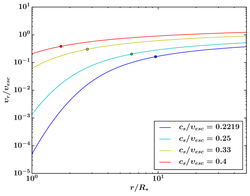
Figure 1.— Flow velocity versus radial distance for four different temperatures, here parameterized by the ratio of the adiabatic sound speed to the escape speed from the star, for one-dimensional, hydrodynamic winds from non-rotating stars. The above profiles are also used as the initial velocity wind profile in our simulations. The circles correspond to the radial distance at which the flow becomes supersonic. Each temperature produces a unique wind acceleration profile and hotter winds always exhibit higher base and terminal velocities than cooler winds.

We use a second-order piecewise linear reconstruction of all the primitive variables ($\rho,\bm{\upsilon},p,\bm{B}$) with minmod limiter, and HLL Riemann solver (e.g. Toro, 2009) to compute the fluxes in equations (3) - (6). The induction equation (eq. 6) is solved with the constrained transport (CT) method (Balsara & Spicer, 1999) in order to ensure that the divergence-free condition for the magnetic field will be maintained in our domain. The computational gird has spherical geometry for the spatial coordinates, and covers $r\in[1,50]R_{*}$, where $R_{*}$ is the stellar radius, and $\theta\in[0,\pi]$, with a total of $256\times 512$ zones. A strecthed grid is constructed along $\widehat{r}$ direction. The first grid zone at the stellar surface (i.e. inner boundary where $r/R_{*}=1$) has size $\Delta r=5\times 10^{-3}R_{*}$ but increases with $r$ such that 256 points reach $50R_{*}$ (i.e. outer boundary), with the last grid cell having size $\Delta r=1.015R_{*}$. The grid is uniform along the $\widehat{\theta}$ direction.

We initialize the whole computational domain with a dipole field, for which the radial, and polar componetnts are given by

$$B_{r}=2B_{*}\left(R_{*}\over r\right)^{3}\cos\theta,$$ (7)

$$B_{\theta}=B_{*}\left(R_{*}\over r\right)^{3}\sin\theta,$$ (8)

where $B_{*}$ is the equatorial surface field strength. We treat the magnetic field using the the ”background field splitting” approach (Powell et al., 1999), which sets the dipole field as a time-independent compenent, and the code calculates the deviation from the initial field. This method provides better numerical accuracy in the treatment of the magnetic field, especially where strong gradients in the magnetic field might otherwise lead to significant numerical diffusion.

We also initialize our grid with a 1D, polytropic, Parker’s wind solution shown in Figure 1, and we set the density and the thermal pressure based on the mass continuity equation and the polytropic relation ($p_{th}\propto\rho^{\gamma}$), respectively. Further details can be found in the following subsection (§3.2).

For both boundary zones of the $\theta$ coordinate we use an ”axisymmetric” type of boundary condition, which symmetrizes all the variables across the borders and flips the signs of the $\phi$ and normal components of the vector fields. The outer boundary condition of $r$ coordinate is set to be ”outflow”, which sets the gradient of each variable to be zero across the boundary. When the code stars to evolve equations (3) - (6) in time, the initial state is blown outwards and the steady-state solution, we are interested in, depends only on the inner boundary conditions. Since our wind solutions only depend on the inner boundary, that represents the stellar surface, for these ghost zones we use a more sophisticated boundary condition. We keep fixed at the stellar boundary the values for the thermal pressure and density computed from the one-dimensional polytropic Parker’s wind, we used to initialize our grid. This boundary condition corresponds to a stellar atmosphere in which its density and temperature do not vary in time and exhibit a temperature profile such that $T\propto\rho^{\gamma-1}$. Moreover, this condition ensures that the temperature of the flow does not exhibit a depedence on $\theta$ at the stellar boundary. The boundary condition for the poloidal magnetic field is forced to maintain the initial dipole state, since the flow is sub-alfvénic and magnetic pressure dominates over the thermal and wind’s hydrodynamic pressure. For the toroidal magnetic field, we linearly extrapolate the toroidal field values calculated in the computational domain into the ghost zones. For the poloidal velocity, we also linearly extrapolate the computed value of the poloidal velocity into the ghost zones, in order to have a flow velocity that increases monotonically with radius inside the ghost zones. In a steady-state and axisymmetric flow, the torroidal component of the electric field should be zero (e.g. Lovelace et al., 1986; Zanni & Ferreira, 2009) and thus we force the poloidal component of the velocity and magnetic field to be parallel to each other. The rotation is enforced only in the stellar boundary, which we accomplish by setting the boundary condition for the toroidal component of the velocity given by the equation:

$$\upsilon_{\phi}=\Omega_{*}r\sin\theta+{\upsilon_{p}\over B_{p}}B_{\phi},$$ (9)

in order to satisfy the $\bm{E}=0$ condition in a frame rotating with the star (Zanni & Ferreira, 2009). In equation (9), $r$ is the spherical radius and the subscripts $p$ and $\phi$ stand for the poloidal and torroidal components respectively, of the velocity and magnetic field.

Each simulation is stopped when the solution converges to a steady-state. Some of the obtained numerical solutions are periodic, and we discuss the steadiness, and the peculiarity of these simulations in Appendix A. We further examine the correctness of each wind solution by checking how well the five constant of motion are conserved along the flow streamlines (e.g. Keppens & Goedbloed, 2000). The numerical accuracy of our simulations is discussed in more detail in Appendix B.

3.2. Parameters of the Study

Table 1Coronal Temperatures of the Parameter Study for Different Stellar Properties

	Temperature ($\textrm{MK}^{\circ}$)	Temperature ($\textrm{MK}^{\circ}$)	Temperature ($\textrm{MK}^{\circ}$)	Temperature ($\textrm{MK}^{\circ}$)
$c_{s}/\upsilon_{esc}$	$M_{*}=1M_{\odot}$	$M_{*}=0.7M_{\odot}$	$M_{*}=0.5M_{\odot}$	$M_{*}=0.2M_{\odot}$
	$R_{*}=1R_{\odot}$	$R_{*}=0.65R_{\odot}$	$R_{*}=0.47R_{\odot}$	$R_{*}=0.22R_{\odot}$
0.2219	1.30	1.40	1.39	1.20
0.25	1.65	1.77	1.77	1.52
0.33	2.88	3.09	3.08	2.66
0.4	4.23	4.53	4.53	3.90

Table 2Simulation Input Parameters and Resulting Global Wind Properties

Case	$c_{s}/\upsilon_{esc}$	$\upsilon_{A}/\upsilon_{esc}$	$\Upsilon$	$<R_{A}>/R_{*}$	$\Upsilon_{open}$	$\Phi_{open}/\Phi_{*}$	$\bar{\mathrm{V}}_{R_{A}}/\upsilon_{esc}$
1	0.2219	0.0151	2.90	3.62	283	0.787	0.0567
2	0.2219	0.0301	11.9	5.52	1020	0.737	0.128
3	0.2219	0.0452	27.7	6.23	1470	0.581	0.146
4	0.2219	0.0753	79.9	7.27	2330	0.430	0.17
5	0.2219	0.105	157	8.07	3170	0.358	0.187
6	0.2219	0.301	1240	11.8	9810	0.224	0.264
7	0.2219	0.627	5980	16.5	25600	0.165	0.335
8	0.2219	0.953	15000	20.2	44300	0.137	0.374
9	0.2219	1.51	41200	25.3	81300	0.112	0.415
10	0.25	0.21	33.2	4.71	1170	0.473	0.206
11	0.25	0.301	69.1	5.47	1820	0.409	0.236
12	0.25	0.627	335	7.83	5070	0.309	0.312
13	0.25	0.953	899	9.83	9460	0.258	0.361
14	0.25	1.51	2720	12.7	18600	0.208	0.413
15	0.25	2.5	8990	16.8	38200	0.164	0.465
16	0.25	4.14	29100	22.0	75700	0.128	0.512
17	0.33	0.953	16.7	3.27	1300	0.704	0.453
18	0.33	2.5	173	5.79	5470	0.448	0.609
19	0.33	3.01	275	6.47	7180	0.406	0.639
20	0.33	4.14	612	7.86	11400	0.344	0.683
21	0.33	6.2	1650	10.1	20700	0.282	0.736
22	0.33	11	6630	14.3	45600	0.209	0.802
23	0.33	17.5	20500	18.6	85000	0.162	0.845
24	0.4	4.14	194	5.68	7900	0.507	0.904
25	0.4	6.2	505	7.27	13800	0.416	0.969
26	0.4	8.6	1090	8.76	20800	0.348	1.01
27	0.4	11	1960	10.2	28800	0.305	1.04
28	0.4	17.5	5890	13.0	50800	0.234	1.10
29	0.4	26	13700	16.4	90400	0.204	1.14
30	0.4	50	62700	22.7	193000	0.140	1.21

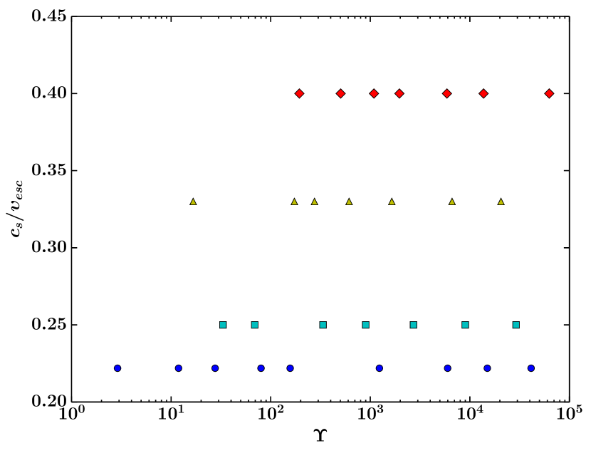
Figure 2.— Parameter space for the 30 simulations in this study. The vertical axis shows parameter $c_{s}/\upsilon_{esc}$, which controls the flow temperarture. The horizontal axis shows the paremeter $\Upsilon$, which is the wind magnetization (see eq 11), and is associated with the average, stellar-surface magnetic field strength. Circles (blue), squares (cyan), triangles (yellow), and diamonds (red) correspond to simulations with $c_{s}/\upsilon_{esc}=$ 0..219, 0.25, 0.33, and 0.4, respectively. Every symbol represents a single case, for which we have a steady-state, wind solution.

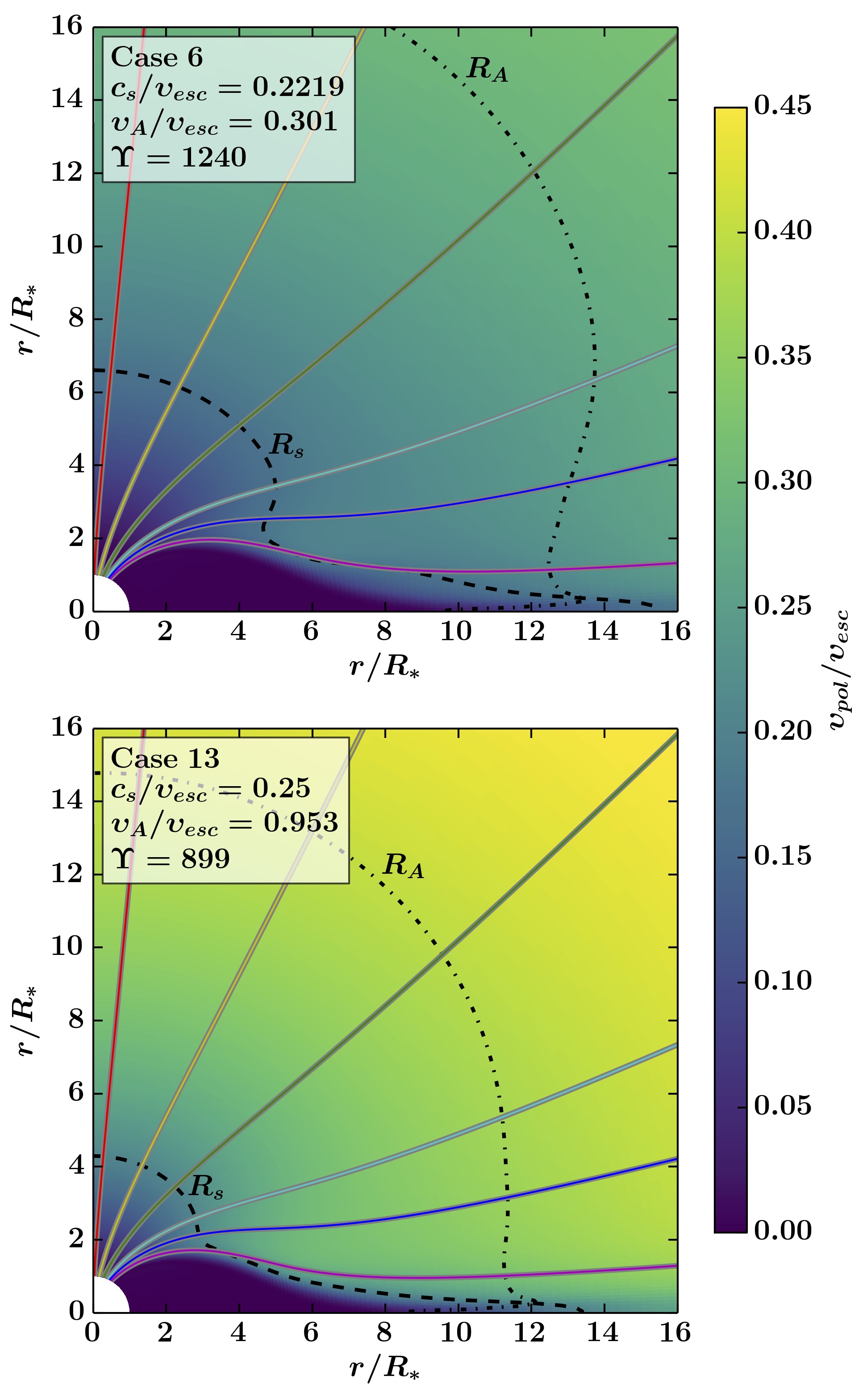
Figure 3.— Poloidal velocity (color scale) with magnetic field lines, for two steady-state wind solutions of this study that demonstrate the two-dimensional structure of the wind and the effect of the temperature on flows with similar magnetization (parameter $\Upsilon$) values. The dashed lines depict the sonic surface and the dotted lines depicts the Alfvénic surface. Each field line is plotted with a different color to indicate the paths along the flow open streamers, plotted in figure 4. The images show only the northern stellar hemisphere and an inner portion of the whole computational domain.

For pure hydrodynamic polytropic stellar winds the two main physical parameters that determine the wind speed and acceleration are the temperature of the plasma and the polytropic index, $\gamma$. In this study we focus on how different coronal temperatures affect the driving of the outflow. The following three dimensionless velocities are the main input parameters of our initial setup: the ratio of the adiabatic sound speed, defined at the stellar surface, to the esacpe speed, $c_{s}/\upsilon_{esc}$, where $c_{s}=\sqrt{\gamma p_{*}/\rho_{*}}$, (”*” symbol denotes values at $R_{*}$), and $\upsilon_{esc}=\sqrt{2GM_{*}/R_{*}}$; the ratio of the Alfvén speed to the escape speed, $\upsilon_{A}/\upsilon_{esc}$, where $\upsilon_{A}=B_{*}/\sqrt{4\pi\rho_{*}}$; the stellar spin rate, $f$, that is the ratio of the stellar equatorial rotation velocity to the break-up speed, where the break-up speed is $\upsilon_{kep}=\upsilon_{esc}/\sqrt{2}$. The latter one will be held fixed for our study close to the solar value, $f=0.00393$. The polytropic index $\gamma$ and the magnetic field geometry are also parameters, but we only vary the dipolar field strengths and we fix $\gamma=1.05$ (Washimi & Shibata, 1993; Matt et al., 2012; Réville et al., 2015a), which behaves like an adiabatically expanding flow that has energy input as the wind expands, such that $p\propto\rho^{1.05}$.

A polytropic treatment of the outflow acceleration is suitable for our purpose because we do not attempt to produce stellar wind solutions that will exhibit plasma properties similar to the ones observed in the solar wind such as speed bimodality, contrast in temperature and density between coronal holes and helmet streamers. Regardless, studies have shown that the polytropic approximation can capture the large-scale structure of the solar-corona magnetic field (see, e.g. Mikić et al., 1999; Riley et al., 2006) and produces wind solutions with velocity profiles that agree with the observed solar wind on large scales (see, e.g. Keppens & Goedbloed, 1999; Ofman, 2004).

Using the ideal-gas equation of state, the stellar coronal temperature can be written in terms of parameter $c_{s}/\upsilon_{esc}$,

$$T_{*}=\left(c_{s}\over\upsilon_{esc}\right)^{2}\left({2GM_{*}\tilde{\mu}m_{p}}\over{\gamma R_{*}k_{B}}\right),$$ (10)

where $k_{B}$ is the Boltzmann constant, $m_{p}$ is the proton mass and $\tilde{\mu}$ is the mean atomic weight (i.e. the average mass per particle measured in units of $m_{p}$). For given stellar parameters, the temperature depends on the mean atomic weight, $\tilde{\mu}$, that is determined by the chemical composition, and the atomic physics of the stellar atmosphere. For a solar-coronal plasma, $\tilde{\mu}=0.6$ (e.g. Priest, 2014), Table 1 translates $c_{s}/\upsilon_{esc}$ in Kelvin, for solar parameters (with $M_{\odot}=1.99\times 10^{33}\textrm{g}$ and $R_{\odot}=6.96\times 10^{10}\textrm{cm}$), and for stars at the age of the Sun, with parameters of $M_{*}=0.7,0.5,0.2M_{\odot}$ and respectively $R_{*}=0.65,0.47,0.22R_{\odot}$, taken from stellar evolution models of Baraffe et al. (1998).

Figure 1 shows velocity profiles of polytropic models for different coronal temperatures, represented in the plot by the dimensionless quantity $c_{s}/\upsilon_{esc}$. Each curve in this plot is the analytic solution of wind speed as a function of radial distance from the stellar surface, and each temperature is indicated by a different color. The plot shows that a hotter wind starts on the stellar surface at a higher speed and also reaches a higher terminal speed. To be more specific, for this range in $c_{s}/\upsilon_{esc}$, the flow speed varies by 3.5 orders of magnitude at $R_{*}$, and by more than a factor of 2 at $50R_{*}$. Morever, a hotter wind accelerates more rapidly compared to a cooler wind, meaning that, at every radius, the hotter wind exhibits a higher value of both $d\upsilon_{r}/dt$ and $d\upsilon_{r}/dr$. Input parameter $c_{s}/\upsilon_{esc}$ varies between 0.2219 and 0.4, a range that was selected to produce reasonable wind velocity profiles for the whole grid of simulations, for a given polytropic index (i.e. $\gamma=1.05$ in our case). This range ensures that the lowest temperature still results in a high enough flow terminal velocity for the wind to be able to escape star’s gravity field. The upper limit for our flow temperature is determined so that it initiates at the stellar corona at subsonic velocities. Our wind solution with $c_{s}/\upsilon_{esc}=0.4$ starts at the bottom of the flow with an initial speed that is already $50\%$ of the sound speed, defined at the stellar surface (see fig. 1), and the wind becomes supersonic at $r=1.7R_{*}$. Higher temperatures will result in outflows with unrealistically high base velocities (i.e. almost supersonic flow at the stellar surafce). Although the polytropic wind formalism includes simplified physics that do not incorporate all relevant coronal processes that drive such outflows, figure 1 shows that the range of winds we consider in our study covers a wide range of wind acceleration profiles, which may encompass the range of velocities encountered in real stellar winds under various coronal conditions.

Table 2 presents the parameters varied ($2^{nd}$ and $3^{rd}$ columns) for all the simulated wind cases in the study. The magnetization of the wind is computed using the formula introduced in Matt & Pudritz (2008),

$${\Upsilon}\equiv{{B_{*}^{2}R_{*}^{2}}\over{\dot{M}_{w}\upsilon_{esc}}},$$ (11)

and the quantity $\Upsilon$ can be regarded as the ratio of the magnetic field energy to the kinetic energy of the flow, or as representing the interplay between the Lorentz forces and the inertia of the wind (ud-Doula & Owocki, 2002). In equation (11), $\dot{M}_{w}$ is extracted dircectly from the simulations, and, for a given surface denisty, depends on the wind-driving physics, the magnetic field structure/configuration, and the numercial setup (for further discussion see Matt et al., 2012, and subsection 4.1). Therefore we choose to present $\Upsilon$ as the second independent variable of the study, even though $\upsilon_{A}/\upsilon_{esc}$ is the input parameter that controls the magnetic field strength. All the values of $\Upsilon$ are listed in the $4^{th}$ column in table 2. The parameter space that has been explored during the entire study is visualized in figure 2, and each simulation is one symbol in this plot. Different symbols and their corresponding colors repesent cases with different temperartures, and overall, we covered 3 to 4 orders of magnitude in wind magnetization for each temperature.

3.3. Wind Velocity Profiles

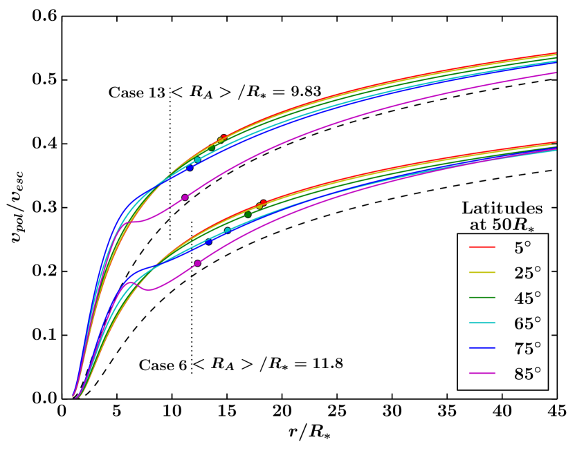
Figure 4.— Wind speed profiles along open field lines at different latitudes, as a function of radial distance, for the cases showed in Figure 3. Each line color correlates with the plotted field lines in Figure 3. For comparison, the dashed lines represent the velocity profiles of pure, one-dimensional hydrodynamic winds. The dotted lines show the torque-averaged Alfvén radius or magnetic lever-arm of the magnetized outflow.

At the start of a simulation, the presence of rotation and magnetic field modifies the initial, spherical symmetric flow, but after some time of evolution the solution relaxes to a steay-state. In order to highlight the influence of the gas temperature on the wind speed in our 2.5D MHD simulations, figure 3 shows the flow poloidal velocity as a color scale on a subset of our domain for two steady-sate wind solutions. Both cases shown have the same order of magnitude in parameter $\Upsilon$. The sonic surface is notated by $R_{s}$ (dashed line) and the Alfvénic surface by $R_{A}$ (dot-dashed line). Open field lines, that correspond to wind streamlines, are also shown. A higher coronal temperature increases the velocity of the flow (bottom panel), and as a result the sonic surface is closer to the stellar surface. The location of the Alfvén surface also comes closer to the star, and this is due to a hotter and faster wind, and also to a slightly lower magnetization of that case (i.e. case 13) relative to top panel case (i.e. case 6).

To show how the wind velocity profile varies with latitude, figure 4 illustrates the poloidal speed versus radial distance, of the plasma flowing along the streamlines of the two cases shown in Figure 3. Each velocity law in figure 4 is individually colored, and matches the colors of the open-field lines plotted in figure 3. The streamlines were chosen to be at various latitudes at $50R_{*}$. The plot comprises two groups of lines, one for each case, and the upper set correspond to the hotter wind (i.e. case 13). Once more, it is clear that the hotter wind accelerates more rapidly and is faster everywhere. An interesting feature shown in Figure 4 is that each field line produces a unique velocity profile. This behavior should be attributed to a different geometrical expansion of flux tubes near the pole and close to the equator, something that originally was pointed out in Pneuman & Kopp (1971). The fact that the 2D wind speed profiles are always faster compared to their 1D hydrodynamic counterparts (black dashed lines) occurs because of the overall, faster-than-$r^{2}$ divergence (i.e. superradial expansion) of the field geometry that channels the flow (e.g. Pneuman, 1966; Kopp & Holzer, 1976; Réville et al., 2016b). Since all of our models are in the slow-magnetic-rotator regime (Belcher & MacGregor, 1976), magneto-centrifugal effects are negligible. We verified that in the absence of rotation wind speed profiles do not change by more than $2\%$ compared with simulated cases from rotating stars. Furthermore, we have observed that, for everything else to be equal, an increase in surface field strength will produce a wind solution that is faster everywhere, (by $\sim 10\%$), also due to a different geometrical expansion of the flux tubes cross-section. The circles in Figure 4 repsresent the location of the local Alfvén radius, the radial distance at which the flow along each field line reaches the local poloidal Alfvén speed. From stellar pole to equator the spherical Alfvén radius decreases because the alfvénic surface reaches the cusp or neutral point of the helmet streamer (closed magnetic loops), that determines the transition region from subalfvenic to superalfvenic flows for streamers adjacent the to the last closed field line (Pneuman & Kopp, 1971). Finally, the black dotted vertical lines depict the size of the effective Alfvén radius. The local $R_{A}$ in each streamline, is always larger compared to $<R_{A}>$, because the latter represents a mean value of the cylindrial Alfvén radius. Comapring the two cases, simulation 13 has a smaller effective lever arm, due to both a higher coronal temperature and a smaller $\Upsilon$ value and this yields a less efficient braking torque on the star.

4. Global Stellar Wind Properties

4.1. Mass and Angular Momentum Outflow Rates

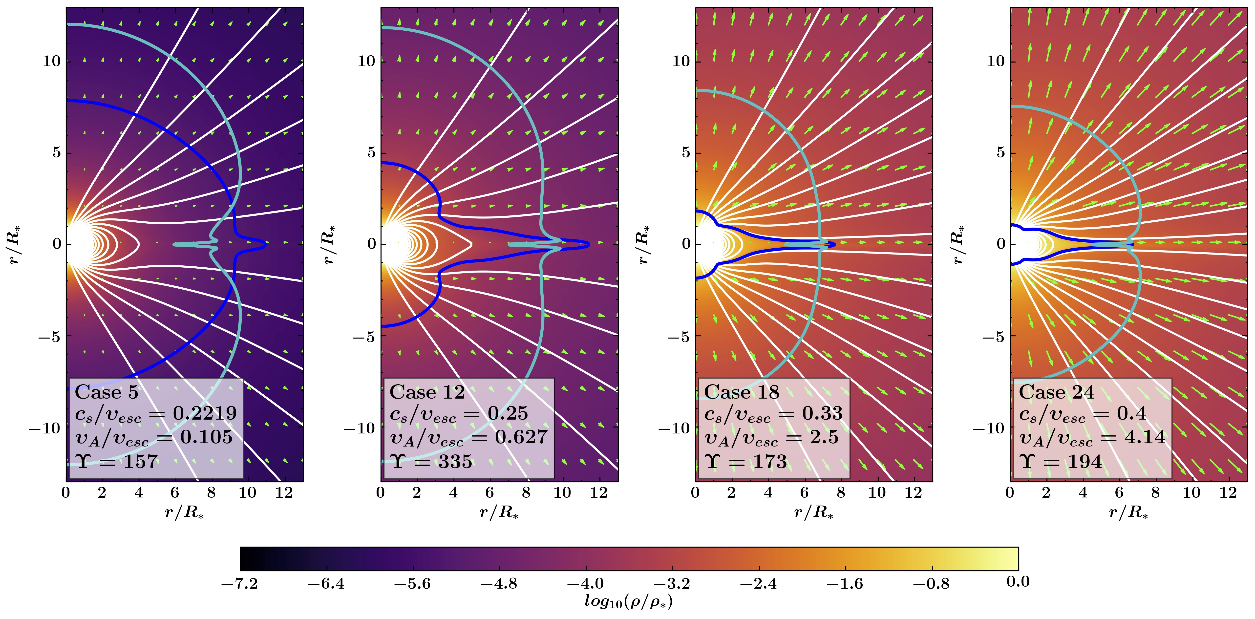
Figure 5.— Colormaps of logarithmic density, magnetic field lines, and velocity vectors, in the inner region of four simulations with similar magnetization, $\Upsilon$, but varying wind temperature (characterized by $c_{s}/\upsilon_{esc}$). The blue and cyan lines show the location of the sonic and the Alfvénic surface, respectively. A higher surface plasma temperature, for about the same value of $\Upsilon$, results in a denser wind and the two critical surfaces being closer to the star.

Figure 5 displays color scale plots of logarithmic density with velocity vectors and magnetic field lines (white lines), for 4 steady-state wind solutions of our study. Each case in figure 5 has the same order of magnitude (and about the same value) in magnetization, but a different plasma temperature. Qualitatively we identify that hotter winds lead to both a smaller sonic surface (blue line) and alfvénic surface (cyan line), as a consequence of being faster everywhere in the grid.

The global outflow rates of mass, $\dot{M}_{w}$, and angular momentum, $\tau_{w}$, are numerically computed for each steady-state wind solution of the study, by using

$$\dot{M}_{w}=\oint_{S}\rho\bm{\upsilon}\cdot d\bm{S},$$ (12)

$$\tau_{w}=\oint_{S}\Lambda\rho\bm{\upsilon}\cdot d\bm{S},$$ (13)

where the integration occurs over any spherical surface that encloses the star, within our computational domain, and

$$\Lambda=r\sin\theta\left(\upsilon_{\phi}-B_{\phi}{B_{p}\over{\rho\upsilon_{p}}}\right).$$ (14)

In the ideal MHD regime, $\Lambda$ gives the specific angular momentum carried away by the wind along a streamline, and is a constant of motion for an axisymmetric, steady-state flow. In practise, we calculate both rates as functions of spherical radius $r$, and use the median values obtained from all the integrated $\dot{M}_{w}(r)$ and $\tau_{w}(r)$ over spherical shells above $10R_{*}$ as global $\dot{M}_{w}$ and $\tau_{w}$. This method avoids numerical diffusion effects that might cause non conservation of mass and angular momentum flux close to the stellar boundary. We then determine the torque-averaged Alfvén radius, $<R_{A}>/R_{*}$, from equation (2), and these are listed in $5^{th}$ column of Table 2.

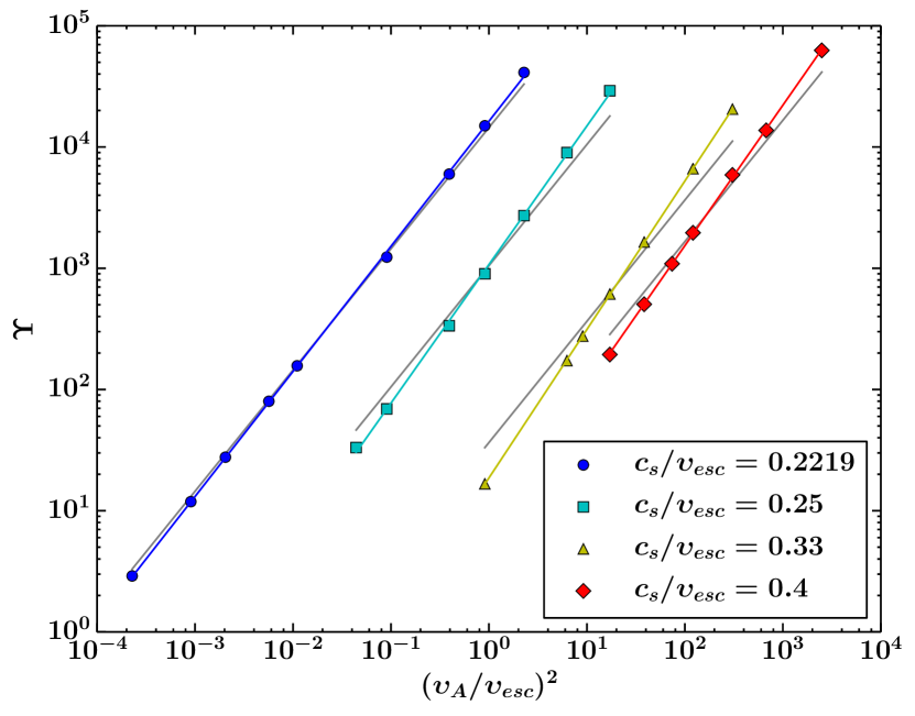
Figure 6.— Wind magnetization, $\Upsilon$, versus square of input parameter $\upsilon_{A}/\upsilon_{esc}$. Same colors/symbols correspond to a grid of simulations with the same value of $c_{s}/\upsilon_{esc}$ (as in Figure 2). In our simulations, $\Upsilon\propto(\upsilon_{A}/\upsilon_{esc})^{2}/\dot{M}_{w}$, and for a given value of $\upsilon_{A}/\upsilon_{esc}$, a hotter wind has have a much higher mass loss rate. Grey scaling laws have a slope of unity. For a given coronal temperature, each scaling law has a slope steeper that unity, indicating that $\dot{M}_{w}$ decreses weakly with an increasing $\upsilon_{A}/\upsilon_{esc}$.

Another way to illustrate the range of the parameter space is to express $\Upsilon$ in terms of the input parameter $\upsilon_{A}/\upsilon_{esc}$. By manipulating equation (11), one can derive that $\Upsilon\propto(\upsilon_{A}/\upsilon_{esc})^{2}/\dot{M}_{w}$, (i.e. $\Upsilon$ depends on $\upsilon_{A}/\upsilon_{esc}$, that controls the surface magnetic field strength, but also is inversely proportional to the stellar mass loss rate, which is an output of the simulations). Figure 6 shows that the four different temperatures of our models follow four different scaling laws of $\Upsilon$ versus the square of $\upsilon_{A}/\upsilon_{esc}$. An increase in $c_{s}/\upsilon_{esc}$ singnificantly affects the stellar mass-loss rates by increasing the speed at the base of the wind. As a consequence $\Upsilon$ decreases, and therefore we have altered the range in field strength (i.e. variation in $\upsilon_{A}/\upsilon_{esc}$) for each temperature in order to achieve about the same range in the wind magnetization for all the temperatures. By doing this, we avoid simulations with a small value of $\upsilon_{A}/\upsilon_{esc}$, and as a consequence a small value of $\Upsilon$, since for such cases the Alfvén surface is very close to the stellar surface. There is no physical reason for not conisdering cases with wind magnetization above $10^{5}$, but these simulations start to become numerically very challenging, due to smaller numerical time-steps and large numerical errors (for further details on the accuracy of the numerical solutions see Appendix B).

The grey lines in Figure 6 correspond to scaling laws with slopes of unity, and show how parameter $\Upsilon$ would depend on $\upsilon_{A}/\upsilon_{esc}$, if the stellar mass loss rate was constant for a grid of simulations with a given coronal temperature, and thus independent of stellar surface magnetic field strength. The fact that we find steeper power-laws, (the slopes are respectively 1.03, 1.14, 1.22, and 1.16 for $c_{s}/\upsilon_{esc}=0.2219,0.25,0.33,0.4$), indicates that the mass loss rates actually decrease with increased field strengths. This feature can be physically explained by an interplay between two competing effects. A stronger field leads to a slightly faster flow (discussed in §3.3), but also to a smaller area on the stellar surface carrying mass flow. Figure 6 indicates that the net result is a slightly decreasing $\dot{M}_{w}$. A similar trend was also seen in Réville et al. (2015a). Nevertheless, we should be cautious in interpreting the scaling laws in figure 6 as realistic stellar mass-loss indicators, since polytropic wind models lack the exact physics that drive outflows from solar- and late-type stars. Early studies in the solar wind (Leer & Holzer, 1980) showed that where the energy is added in the flow has a big influence on the resulting solar mass loss rate. Moreover latest theoretical models (Cranmer & Saar, 2011; Suzuki et al., 2013), suggest that a realistic treatment of coronal heating is needed for accurate predictions on stellar mass loss rates from cool stars. Therefore, the scaling laws between $\Upsilon$ and $\upsilon_{A}/\upsilon_{esc}$ can be interpreted as a part of the generic phenomenology in our simulations, and should not be regarded as trends that give accurate predictions on mass loss rates in solar- and late-type stars. Still our formulae shall provide the exerted magnetic torque for any given $\dot{M}_{w}$, extracted from observations (e.g. Wood et al., 2002, 2014) or modeling (e.g. Holzwarth & Jardine, 2007; Cranmer & Saar, 2011; Suzuki et al., 2013).

4.2. Scaling Laws Between Alfvén Radius and $\Upsilon$

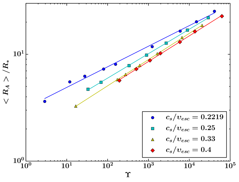
Figure 7.— The dependence of the effective Alfvén radius, $<R_{A}>/R_{*}$, on $\Upsilon$ for all the cases of the parameter study. The colors/symbols have the same meaning as in Figure 2. Four simple power laws of $<R_{A}>/R_{*}$ on parameter $\Upsilon$ are shown, and each one corresponds to a different value of $c_{s}/\upsilon_{esc}$. For a given $\Upsilon$, the magnetic lever arm (i.e. $<R_{A}>/R_{*}$) of the wind decreases, with an increasing coronal temperature, and as a consequence the torque exerted on the star becomes less efficient.

The dependence of the effective Alfvén radius, $<R_{A}>/R_{*}$ on wind magnetization, $\Upsilon$, for all the numerical solutions of the study is depicted in figure 7. Each point in Figure 7 corresponds to a single simulation, and the color and symbols have the same meaning as in figure 6. In order to fit the simulation data, we use the formulation introduced in Matt & Pudritz (2008), that scales $<R_{A}>/R_{*}$ as a power law in $\Upsilon$,

$${{<R_{A}>}\over{R_{*}}}=K_{s}\Upsilon^{m_{s}},$$ (15)

where $K_{s}$ and $m_{s}$ are dimensionless fitting constants, and equation (15) determines $<R_{A}>/R_{*}$ in terms of the magnetic field strength on the stellar surface. Four different fitting laws are shown in Figure 7, and the values of $K_{s}$ and $m_{s}$ for every fit are given in $2^{nd}$ and $3^{rd}$ column of Table 3.

Each value of $c_{s}/\upsilon_{esc}$ gives a simple power law of the torque-averaged Alfvén radius on $\Upsilon$ for various surface magnetic field strengths. However the fit parameters are different with each coronal temperature. The power law for $c_{s}/\upsilon_{esc}=0.2219$ is shallower, (see also Table 3), compared with previous parameter studies (Matt et al., 2012; Réville et al., 2015a), and can be understood as an effect due to differences in the numerical setup between the studies (e.g. geometry of the problem, numerical scheme, different approach on boundary conditions), indicative of systematic errors. Réville et al. (2015a) demonstrated different power laws resulted from different field geometries. It was also shown that the compexity of the magnetic field does not significantly influence the wind acceleration. For this study only dipolar fields are considered, but by varying the gas temperature, we actually change the acceleration of the flow. As a consequence the wind speed also changes, for simulations with different values of $c_{s}/\upsilon_{esc}$, and that physically explains the four power laws in Figure 7. In conclusion, hotter winds are faster, and thus, the Alfvén surface comes closer to the star, the size of the lever arm or the effective Alfvén radius decreases, and therefore the magnetic braking torque that is exerted on the star becomes weaker.

4.3. Scaling Laws Using the Amount of Open Magnetic Flux

In Réville et al. (2015a) an alternative formulation for the torque-averaged Alfvén radius was introduced, that scales $<R_{A}>/R_{*}$ as a power law in a new $\Upsilon$-like parameter that depends on the amount of open magnetic flux, (see also Washimi & Shibata, 1993). In general, the unsigned magnetic flux of the stellar magnetic field, as a function of spherical radius $r$, can be evaluated as,

$$\Phi(r)=\oint_{S}|\bm{B}\cdot d\bm{S}|,$$ (16)

where the integration is performed over sperical surfaces that enclose that star. For a given field geometry, dipole in our case, magnetic flux intitially drops as $1/r$, but there is a regime in which the thermal pressure and the inertia of the wind dominates over the magnetic stresses, the field completely opens and the magnitude of the magnetic flux becomes constant (i.e. open magnetic flux), see for example figure 5 in Réville et al. (2015a).

Following Réville et al. (2015a), the new $\Upsilon$-like parameter, is defined as,

$${\Upsilon_{open}}\equiv{{\Phi_{open}^{2}}\over{R_{*}^{2}\dot{M}_{w}\upsilon_{esc}}},$$ (17)

where $\Phi_{open}$ is the open magnetic flux that is directly computed from the numerical simulations by equation (16). We use as $\Phi_{open}$, for a given wind solution, the median value of $\Phi(r)$ above the corresponding $<R_{A}>/R_{*}$ of that solution, where we have identified that magnetic flux is constant. The $6^{th}$ column in Table 2 lists all the values of $\Upsilon_{open}$. The $7^{th}$ column in Table 2 contains all the values of the fractional open flux (i.e. $\Phi_{open}$ normalized to the surface unsigned magnetic flux, $\Phi_{*}$), which can be written as $\Phi_{open}/\Phi_{*}=(\Upsilon_{open}/\Upsilon)^{1/2}/(4\pi)$.

The value of $<R_{A}>/R_{*}$ versus parameter $\Upsilon_{open}$, for the entire study, is presented in figure 8. Similarly to equation (15), a function in the form of

$$<R_{A}>/R_{*}=K_{o}\Upsilon_{open}^{m_{o}}$$ (18)

fits tha data, and again $K_{o}$ and $m_{o}$ represent dimensionless fitting constants and $<R_{A}>/R_{*}$ is determined here in terms of the open magentic flux. Four power laws are shown in Figure 8, and the $5^{th}$ and $6^{th}$ column in Table 3 lists the values of the fitting constants for each scaling law. The figure demonstrates, how effective Alfvén radius scales as a simple braking law with parameter $\Upsilon_{open}$, for every value of $c_{s}/\upsilon_{esc}$. Furthermore, Figure 8 reveals one of the key result in this parameter study. We show that the temperature of the flow, which affects the wind velocity and acceleration profile, is an important parameter in the magnetic-braking models. Réville et al. (2015a) showed that all the wind solutions in their study followed one unique power law, demonstrating that the $<R_{A}>/R_{*}$-versus-$\Upsilon_{open}$ scaling was independent of the field geometry, but they assumed a fixed stellar coronal temperature. The fact that our power law, for $c_{s}/\upsilon_{esc}=0.2219$, is steeper (see also Table 3), compared to the single braking law found in Réville et al. (2015a), might be explained as an effect due to different choices in the numerical setups of the two studies, as discussed in the previous subsection. An influence on the braking laws, due to a different coronal temperature has also been observed in Réville et al. (2016a). In conclusion, the temperature of the flow affects the size of the magnetic lever-arm (i.e. $<R_{A}>/R_{*}$), and the efficiency of magnetic braking.

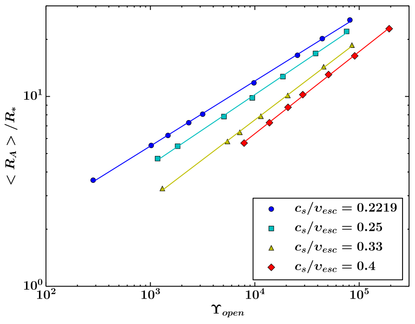
Figure 8.— Effective Alfvén radius, $<R_{A}>/R_{*}$, versus the parameter $\Upsilon_{open}$ (eq. 18) for all the simulations of the study. Colors/symbols are the same as in figure 2. Four different fitting laws are shown, one for each set of wind solutions with a given value of $c_{s}/\upsilon_{esc}$. An increase in the temperature of the flow, for winds with the same value of $\Upsilon_{open}$, results in an increase of the size of $<R_{A}>/R_{*}$ and the efficieny of the braking torque.

Table 3Fitting Constants of the Parameter Study

$c_{s}/\upsilon_{esc}$	$K_{s}$	$m_{s}$	$1/(4+q)$	$K_{o}$	$m_{o}$	$1/(2+q)$	$K_{q}$	$q$
0.2219	3.1 $\pm$ 0.1	0.193 $\pm$ 0.005	0.202 $\pm$ 0.004	0.51 $\pm$ 0.01	0.343 $\pm$ 0.003	0.34 $\pm$ 0.01	0.023 $\pm$ 0.005	0.94 $\pm$ 0.09
0.25	2.08 $\pm$ 0.02	0.229 $\pm$ 0.001	0.218 $\pm$ 0.002	0.34 $\pm$ 0.01	0.370 $\pm$ 0.004	0.386 $\pm$ 0.006	0.088 $\pm$ 0.009	0.59 $\pm$ 0.04
0.33	1.64 $\pm$ 0.01	0.246 $\pm$ 0.001	0.230 $\pm$ 0.002	0.160 $\pm$ 0.007	0.418 $\pm$ 0.004	0.426 $\pm$ 0.006	0.32 $\pm$ 0.02	0.35 $\pm$ 0.03
0.4	1.63 $\pm$ 0.04	0.240 $\pm$ 0.003	0.2378 $\pm$ 0.0005	0.118 $\pm$ 0.006	0.433 $\pm$ 0.005	0.454 $\pm$ 0.002	0.64 $\pm$ 0.01	0.205 $\pm$ 0.009
0.2219	2.49	0.2177	-	-	-	-	-	-
0.2219	2.0 $\pm$ 0.1	0.235 $\pm$ 0.007	0.21	0.65 $\pm$ 0.05	0.31 $\pm$ 0.02	0.37	-	0.7

5. Magnetic braking laws for known wind acceleration profile

5.1. Semi-analytic Model for Alfvén Radius versus $\Upsilon_{open}$

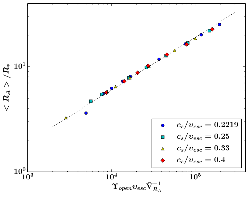
Figure 9.— Effective Alfvén radius, $<R_{A}>/R_{*}$, versus the quantity $\Upsilon_{open}\upsilon_{esc}\bar{\mathrm{V}}_{R_{A}}^{-1}$ for all the simulation data. Colors/symbols have the same meaning as in Figure 2. All the data points collapse in a single braking law, compared to Figure 8. The slope (or power-law index) of the dotted line is fixed to $1/2$, and fits the data according to equation (26).

We showed above that the flow temperature and the resulting wind acceleration can influence the effieciency of the braking toque. For this section, our objective is to provide a more generic braking law that will take this effect into account.

In order to mathematically express the dependence of the braking laws on the acceleration profile of the flow, we will employ similar one-dimensional analysis that was used in earlier works (e.g Kawaler, 1988; Tout & Pringle, 1992; Matt & Pudritz, 2008; Réville et al., 2015a). For a one-dimensional, MHD flow, along a magnetic flux tube, the wind velocity at the Alfvén radius, by defintion, is equal to the local Afvénic speed. This is

$$\upsilon^{2}(R_{A})=\upsilon_{A}^{2}={B_{A}^{2}\over{4\pi\rho_{A}}},$$ (19)

where $B_{A}$ and $\rho_{A}$ are the local magnetic field and density respectively, at the Alfvén surface. In order to evaluate $B_{A}$ at $R_{A}$, one must specify how the magnetic field stength depends on radius. Hence, for this work, we adopt a prescription similar to Mestel & Spruit (1987, see also ()), in which the magnetic field is approximated as having two regions. The inner region exists from the stellar surface out to the ”open-field” radius, $R_{o}$, in which the field is a single power law in radius,

$$B(r\leq R_{o})=B_{*}\left({R_{*}\over r}\right)^{l+2},$$ (20)

with $l=1$ for a dipole. The outer region lies above $R_{o}$ in which the field decreases as a monopole, (i.e. $l=0$),

$$B(r\geq R_{o})=B_{o}\left({R_{o}\over r}\right)^{2},$$ (21)

where $B_{o}$ denotes $B(R_{o})$, given by equation (20). We also assume that the flow is the same along every field line (i.e. all values are only a function of radius and not latitude) and in a steady-state.

This treatment for the stellar field magnetic is a simple approximation for the real magnetic field configurations in a wind, where near the star, the field closely resembles the potential field, and further out, it is stretched to a nearly radial configuration by the flow (see for example fig. 5). For a detailed comparison of the magnetic field in a wind simulation with a potential and radial field, see Réville et al. (2015b).

In all our simulations the Alfvén surface is located at the open-field region, and therefore, we assume that the condition $R_{A}>R_{o}$ holds for all our cases as if they were 1D flows. Then, by combining equations (20) and (21), the magnetic field strength at $R_{A}$ can now be written

$$B_{A}=B_{o}\left({R_{o}\over R_{A}}\right)^{2}=B_{*}\left({R_{*}\over R_{o}}\right)^{l+2}\left({R_{o}\over R_{A}}\right)^{2}.$$ (22)

Since magnetic flux is conserved, it can be written at the Alfvén radius as

$$\Phi_{A}=4\pi R_{A}^{2}B_{A}=4\pi R_{o}^{2}B_{o}=\Phi_{open},$$ (23)

which equals the total open flux in the wind. By combining equations (17), (19), and (23), we get

$$\left(R_{A}\over R_{*}\right)^{2}={1\over(4\pi)^{2}}\Upsilon_{open}{\upsilon_{esc}\over\upsilon(R_{A})},$$ (24)

where we have used $\dot{M}_{w}=4\pi\rho_{A}R_{A}^{2}\upsilon(R_{A})$, for a spherical symmetric flow in the open-field region.

Since our wind solutions are multi-dimensional, we can associate the terms $R_{A}/R_{*}$ and $\upsilon(R_{A})$ in equation (24) with the torque-averaged Alfvén radius, $<R_{A}>/R_{*}$ and $\bar{\mathrm{V}}_{R_{A}}$, where $\bar{\mathrm{V}}_{R_{A}}$ represents the average wind speed at the Alfvén surface. We define

$$\bar{\mathrm{V}}_{R_{A}}\equiv{\sum\limits_{i}^{N}\upsilon[(R_{A})_{i},\theta_{i}],\over N},$$ (25)

where the sum is over each discretized grid point $i$ along the Alfvén surface. $\bar{\mathrm{V}}_{R_{A}}$ is computed individually for each case in the study, and the values are listed in the $8^{th}$ column in Table 2.

Following equation (24), we plot $<R_{A}>/R_{*}$ versus the new quantity, $\Upsilon_{open}\upsilon_{esc}\bar{\mathrm{V}}_{R_{A}}^{-1}$, as depicted in Figure 9, and fit the data to the function

$${<R_{A}>\over R_{*}}=K_{c}\left(\Upsilon_{open}{\upsilon_{esc}\over\bar{\mathrm{V}}_{R_{A}}}\right)^{1/2},$$ (26)

where again $K_{c}$ is introduced as a dimesionless fitting constant and its value should only deviate from $1/(4\pi)$ due to 2D effects, neglected in equation (24). The best-fit value for $K_{c}$ gives

$$K_{c}=0.7540\left(1\over 4\pi\right)\pm 0.0004.$$ (27)

By including in our torque formalism, the dimensionless term $\upsilon_{esc}/\bar{\mathrm{V}}_{R_{A}}$, that contains all the information regarding the velocity and acceleration profile of the outflow, all the data points in figure 9 collapse in one single and precise power-law. Hence, equation (26) predicts the effective Alfvén radius of any wind, as long as $\bar{\mathrm{V}}_{R_{A}}$ and $\Upsilon_{open}$ are known.

5.2. Power-law Approximation for Wind Velocity at the Alfvén Radius, $\bar{\mathrm{V}}_{R_{A}}$

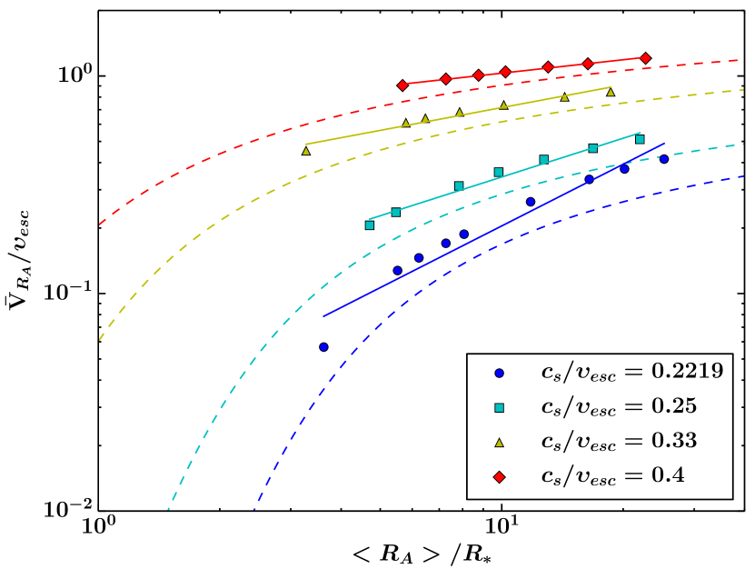
Figure 10.— Average flow speed at the Alfvén surface, $\bar{\mathrm{V}}_{R_{A}}$, versus $<R_{A}>/R_{*}$ for all the simulated cases of the study. Colors/symbols are the same as in Figure 2. Each point in this plot represents the average wind speed at the Alfvén radius of a single wind solution (eq. 25). The solid lines represent the equation (28) with fit parameters listed in Table 3. For comparison, the dashed lines show the normalized radial velocity, $\upsilon_{r}/\upsilon_{esc}$, as a funcion of $r/R_{*}$, of the 1D, hydrodynamic, winds illustrated in Figure 1.

Equation (26) can naturally explain the simple power laws in figure 8, if wind speed, $\bar{\mathrm{V}}_{R_{A}}$, is also a power-law in $<R_{A}>/R_{*}$ but with a scaling that varies for each temperature. To verify this, we plot $\bar{\mathrm{V}}_{R_{A}}$ versus the torque-averaged Alfvén radius, $<R_{A}>/R_{*}$, for all the simulations in figure 10. For comparison, the velocity profiles of the polytropic, Parker wind models, shown in Figure 1, are also plotted. We fit a power-law function to the data, given by

$${\bar{\mathrm{V}}_{R_{A}}\over\upsilon_{esc}}=K_{q}\left(<R_{A}>\over R_{*}\right)^{q}$$ (28)

where $K_{q}$ and $q$ are both dimensionless fitting constants, related to the acceleration profile of the wind. Each temperarture gives us a seperate pair of $K_{q}$ and $q$, tabulated in the $8^{th}$ and $9^{th}$ column of Table 3, respectively. The value of $q$, found in Réville et al. (2015a), is also given in Table 3.

It is clear that equation (28) is valid as a first order approximation, despite the fact that the simulated winds do not follow a perfect power law (solid lines in fig. 10) and the behavior of $\bar{\mathrm{V}}_{R_{A}}$, as a function of $<R_{A}>/R_{*}$, exhibit a similar shape to 1D, hydrodynamic winds of the same value of $c_{s}/\upsilon_{esc}$ (dashed lines in fig. 10). Perhaps, for even more precise stellar-torque formulae, a different velocity law could be applied (e.g. modified beta-law, see for example Lamers & Cassinelli (1999)). Nonetheless, over a small range of radii, these trends can be approximated by a power law, and that approximate fit, explains the power-law behavior in figure 8. In addition, working with equation (28), one can analytically solve equation (26) for $<R_{A}>/R_{*}$, (see below).

Another interesting trend in figure 10 is that the plotted data points are noticeably above the hydrodynamic wind velocity profiles. This can be understood as an effect due to both, the differences in the dynamics of the two flows (i.e. MHD versus HD flow) as discussed in section 3.3, and the specific way the averaging and the scaling was done in equation (28). Figure 10 also indicates why the braking laws in figures 7 and 8 start to converge, for higher coronal temperatures (e.g. the yellow and red lines with $c_{s}/\upsilon_{esc}=0.33,0.4$). Hotter flows enter the regime where the wind speed starts to saturate to wind terminal speed (i.e. speed at infinity), in a shorter radial distance compared to cooler winds. Hence, outflows that approach an almost constant speed, suggest a $q$ that asymptotes to zero. Lastly, we found two empirical functions, which predict fitting constants $K_{q}$ and $q$ over any continuous range of values of $c_{s}/\upsilon_{esc}$. These functions are,

$$K_{q}=1.36[5.87(c_{s}/\upsilon_{esc})^{2}-1.18(c_{s}/\upsilon_{esc})],$$ (29)

$$q=0.932[0.000979(c_{s}/\upsilon_{esc})^{-4.51}$$

$$+\ 0.553(c_{s}/\upsilon_{esc})].$$ (30)

The method and the derivation of equations (29) and (5.2) exist in Appendix C.

By combining equations (26) and (28), we obtain

$${<R_{A}>\over R_{*}}=\left({K_{c}^{2}\over K_{q}}\Upsilon_{open}\right)^{1/(2+q)}.$$ (31)

An interesting characteristic of equation (31) is that it explains the fitting constants of equation (18) in terms of other fitting constants, and consists of an analytic expression for the effective Alfvén radius. This formalism is independent of the temperature of the flow (but requires a known wind acceleration profile), the geometry of the magnetic field, and predicts the torque exerted on the star for any value of $\Upsilon_{open}$, for a given rotation rate (in the slow-rotator regime) and polytropic index ($\gamma=1.05$ in this study). Comparing equations (18) and (31), we identify that $K_{o}\sim(K_{c}^{2}K_{q}^{-1})^{1/(2+q)}$ and $m_{o}\sim 1/(2+q)$. The predicted values of $m_{o}$ for each temperature, are listed in the $7^{th}$ column in Table 3. Clearly $m_{o}$ and $K_{o}$ stongly depend on the accelaration profile of the wind, here parametrized with $K_{q}$ and $q$.

5.3. Semi-analytic Model for Alfvén Radius versus $\Upsilon$

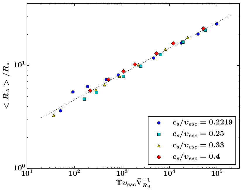
Figure 11.— $<R_{A}>/R_{*}$ versus the quantity $\Upsilon\upsilon_{esc}\bar{\mathrm{V}}_{R_{A}}^{-1}$ for all the simulations. Colors/symbols have the same meaning as in Figure 2. All the data points are fitted by a single coefficient $K_{l}$, and the fitting line (dotted line) has a slope (or power-law index) of $1/4$, according to equation (33). The small spread of the data points, observed in this braking law is primarily due to variations in the ratio of the Alfvén radius to the open-field radius (see also eq. 32 and Figure 12).

The formalism given by equation (26) provides an excellent fit, in terms of predicting the torque-averaged Alfvén radius from parameter $\Upsilon_{open}$, for a given wind acceleration. However, in real wind cases, the amount of open magnetic flux is a quantity that is not observable, and can only be predicted (e.g. Vidotto et al., 2014a; Réville et al., 2015b; See et al., 2017). Therefore, in this section, we aim at extracting trends for the braking torque based on $\Upsilon$, that depends on the surface magnetic field strength (or surface magnetic flux).

Such trends can be obtained analytically, by combining equations (22), (23), (24), and also by using the definition for $\Upsilon$, (eq. 11), which yields

$$\left(R_{A}\over R_{*}\right)^{2l+2}\left(R_{o}\over R_{A}\right)^{2l}=\Upsilon{\upsilon_{esc}\over\upsilon(R_{A})}.$$ (32)

Figure 11 shows the effective Alfvén radius versus the $\Upsilon$-based quantity, $\Upsilon\upsilon_{esc}\bar{\mathrm{V}}_{R_{A}}^{-1}$, as it is suggested by equation (32). Once more, all the details regarding the acceleration of the flow have been contained in the dimensionless term, $\upsilon_{esc}/\bar{\mathrm{V}}_{R_{A}}$, and as a result all the simulations lie close to a single power law. By solving equation (32) for $R_{A}/R_{*}$, the power on this braking law depends only the geometry of the field (or $l$). Hence, this should apply to more complex field geometries as well, but for our case, with a dipole field ($l=1$), the slope, of the single line formed by the data points in Figure 11, is equal to $1/4$. Following this simplified analysis, we fit the data in Figure 11 with

$${<R_{A}>\over R_{*}}=K_{l}\left(\Upsilon{\upsilon_{esc}\over\bar{\mathrm{V}}_{R_{A}}}\right)^{1/4},$$ (33)

and $K_{l}$ is introduced as the only fitting constant. The best-fit value of $K_{l}$ is

$$K_{l}=1.46\pm 0.02.$$ (34)

Fitting constant $K_{l}$ includes any factors, due to the multidimensionality of our simulations, and most important, the comparison between equations (32) and (33) suggests that $K_{l}$ also includes the dimensionless ratio of the Alfvén radius to the open-field radius of the wind, $R_{A}/R_{o}$. Furthermore, the fact that all the data points do not precisely lie along the single power law in Figure 11, implies that the term $R_{A}/R_{o}$ is not constant for all the simulations and exhibits a dependence on the flow temperature.

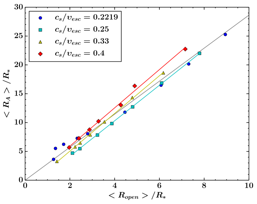
Figure 12.— Torque-averaged Alfvén radius, $<R_{A}>/R_{*}$, versus the normalized open-field radius, $<R_{o}>/R_{*}$. Color/symbols are the same as in figure 2. The grey line shows a linear function that represents all the data, and gives $<R_{A}>/<R_{o}>=2.86$. Cyan, yellow, and red solid lines depict linear functions as well, as an example, to show how $<R_{A}>/<R_{o}>$ systematically varies for each temperature.

A coherent way to estimate the open-field radius (i.e. the radial distance in which the wind’s thermal and ram pressure overpower the magnetic field pressure, and as a result the unsigned magnetic flux becomes constant as a function of radial distance) for all our simulations, is to define $<R_{o}>/R_{*}$ as

$$\left({<R_{o}>\over R_{*}}\right)^{l}\equiv{\Phi_{*}\over\Phi_{open}}.$$ (35)

In other words, equation (35) gives the radial distance in which the function, $\Phi(r)/\Phi_{*}=(R_{*}/r)^{l}$, intersects the line, $\Phi(r)/\Phi_{*}=\Phi_{open}/\Phi_{*}=\textrm{const.}$, and applies for any given single magnetic field geometry.

In Figure 12, we present the normalized open-field radius, $<R_{o}>/R_{*}$, versus the torque-averaged Alfvén radius, $<R_{A}>/R_{*}$, and the plot shows that all the simulations have approximately the same ratio, $<R_{A}>/<R_{o}>$. This feature explains why equation (33) successfully represents the data. Assuming a linear scaling between $<R_{A}>$ and $<R_{o}>$, yields $<R_{A}>/<R_{o}>\approx 2.86$. A closer inspection reveals a range in $<R_{A}>/<R_{o}>$ between 2.23 and 4.07, that will produce a scatter in figure 11 only as the square root of this ratio, with the most extreme deviation from the linear function (grey line) to be $20\%$. In fact, $<R_{A}>/<R_{o}>$ systematically changes, which explains the systematic scatter in figure 11 as due to small differences in $<R_{A}>/<R_{o}>$ for each temperature. The general trend in figure 12, is that $<R_{A}>/<R_{o}>$ increases for an increasing flow temperature (see solid cyan, yellow, and red lines), though that is not the case for simulations with $c_{s}/\upsilon_{esc}=0.2219$, for which the data points exhibit a peculiar behavior. Lastly, $<R_{A}>/<R_{o}>$ should exhibit a dependence on the geometry of the field, and in particular, the expected trend is that for an increasing complexity in the field geometry, this ratio reduces (see Finley & Matt, 2017).

Equation (33) can be further expanded by substituting $\bar{\mathrm{V}}_{R_{A}}$ with the velocity law, given by equation (28), which yields

$${<R_{A}>\over R_{*}}=\left({K_{l}^{4}\over K_{q}}\Upsilon\right)^{1/(4+q)}.$$ (36)

Equation (36) explains the fitting constants of equation (15) in terms of other fitting constants, and represents an analytic formula of the torque-averaged Alfvén radius for any value of parameter $\Upsilon$, for any known wind acceleration profile (known values of $K_{q}$ and $q$), for a dipolar field geometry, for a star that is a slow rotator, and for $\gamma=1.05$.

Finally, equation (36) can work as a proxy in order to extract predictions for the values of $K_{s}$ and $m_{s}$ (see eq. 15), that determine the simple power laws in figure 7. It is expected that $K_{s}\sim(K_{l}^{4}/K_{q})^{1/(4+q)}$ and $m_{s}\sim 1/(4+q)$, see for example the $4^{th}$ column in Table 3, for the predicted values of $m_{s}$, for each flow temperature. Undoubtedly, the primary reason for the differences in the four different power laws in figure 7, is related to the acceleration of the flow, which depends on the stellar coronal temperature.

6. Summary and Conclusions

Employing 2.5D, ideal MHD, axisymmetric numerical simualtions, we provide the first systematic study on how the thermodynamic conditions (i.e. flow temperature for the current work), in stellar coronae of cool stars, can influence the losses of stellar angular momentum due to magnetized winds. Our parameter space considers polytropic flows, modified with rotation and magnetic fields, includes 30 steady-state wind solutions (see Appendix D for color scale plots of the complete simulation grid), and quantifies the braking torque for 4 different coronal temperatures, over a wide range of magnetic field strengths, for slow rotators, for dipolar fields, and for a fixed polytropic index ($\gamma=1.05$). The following points summarize the main conclusions in this work:

1. For a given value of wind magnetization, $\Upsilon$, (or a given value of $\Upsilon_{open}$), a hotter wind is faster, reaches the Alfvén speed closer to the star and, as a consequence, the torque exerted on the surface of the star decreases.

2. We present two formulae that estimate the size of the torque-averaged Alfvén radius: one that depends on parameter $\Upsilon$, which is based on stellar-surface parameters, and a second one that depends on $\Upsilon_{open}$, which is based on the amount of open magnetic flux. Each formulation gives a simple power law for each coronal temperature. By substituting equation (15) into equation (2), the stellar angular-mometum-loss rate due to a magnetized wind is

   $$\tau_{w}=K_{s}^{2}\Omega_{*}\upsilon_{esc}^{-2m_{s}}\dot{M}_{w}^{1-2m_{s}}R_{*}^{2+4m_{s}}B_{*}^{4m_{s}},$$ (37)

   which is useful if the dipole field strength at the stellar surface is known. Similarly, by combining equations (2) and (18), we have

   $$\tau_{w}=K_{o}^{2}\Omega_{*}\upsilon_{esc}^{-2m_{o}}\dot{M}_{w}^{1-2m_{o}}R_{*}^{2-4m_{o}}\Phi_{open}^{4m_{o}},$$ (38)

   which is useful if the amount of the total open magnetic flux is known. The above relations can be used for studies of the rotational evolution of cool stars, and predict the torque on stars with dipolar magnetic fields, that are slow rotators, and exhibit coronal winds with $\gamma=1.05$. Four different flow temperatures were studied, and the values of fitting constants, $K_{s},m_{s},K_{o},m_{o}$ for each temperature, can be found in Table 3.

3. Using a simplified analysis (in §5), we identified that the wind acceleration profile is a key factor that determines how the torque scales with parameter $\Upsilon$ or $\Upsilon_{open}$. We found (in Figures 9 and 11) that by including the dimensionless velocity term, $\upsilon_{esc}/\bar{\mathrm{V}}_{R_{A}}$, ($\bar{\mathrm{V}}_{R_{A}}$ is the wind’s mean speed at the Alfvén surface), in each of the two torque formulae, all the simulation data collapse into a unique power law, independent of the flow temperature. In other words, we propose that a key term that needs to be included in stellar-torque prescriptions when one considers stars with different coronal conditions (and consequently different wind acceleration profiles) is the average wind speed at the Alfvén surface, whatever heats and expands the outflow. This conclusion should be independent of the actual wind temperature or details of how the wind is driven, since the angular momentum flux primarily depends on the flow velocity, mass density, and the magnetic field properties (see e.g., eqns 13 and 14).

4. By considering a power-law dependence of $\bar{\mathrm{V}}_{R_{A}}$ (i.e. wind’s mean speed at the Alfvén surface) in $<R_{A}>/R_{*}$, the torque-averaged Alfvén radius can be expressed with an analytic form (see eqs 31, 36), for a well-aproximated (or known) wind acceleration profile. Equations (2), (36), and (2), (31), then yield respectively,

   $$\tau_{w}={K_{l}^{8/(4+q)}\over K_{q}^{2/(4+q)}}\Omega_{*}\upsilon_{esc}^{-2/(4+q)}\dot{M}_{w}^{(2+q)/(4+q)}$$

   $$\times R_{*}^{(12+2q)/(4+q)}B_{*}^{4/(4+q)},$$ (39)

   and

   $$\tau_{w}={K_{c}^{4/(2+q)}\over K_{q}^{2/(2+q)}}\Omega_{*}\upsilon_{esc}^{-2/(2+q)}\dot{M}_{w}^{q/(2+q)}$$

   $$\times R_{*}^{2q/(2+q)}\Phi_{open}^{4/(2+q)}.$$ (40)

   These equations are sucessors to equations (37), (38), since they drop the dependence of magnetic braking on the flow temperature. Thus, equations (4), and (4) should predict stellar torques for any given coronal temperature, but require the wind acceleration profile to be known. The values of fitting constants $K_{q},q$, that determine the acceleration of the outflow, for the temperatures examined in this study, can be found in table 3 (see also Appendix C for predictions on the values of these fitting constants over a continuous range of temperartures), and the values of $K_{c}$, $K_{l}$ exist in subsections 5.1 and 5.3, respectively.

In order to give an example of how our formulation can be used, we apply it to the solar case. In general, the torque exerted on the Sun (or any star) is an integrated quantity, and its value depends on a sum over the local values of the angular momentum flux (see eqn 13). During the solar minimum the solar wind comprises two components, a fast and a slow wind (see also §1). Our wind models do not produce a bimodal outflow, and thus, we expect that our estimated solar torque should lie somewhere in-between the torques predicted by our fastest (i.e. with $c_{s}/\upsilon_{esc}=0.4$) and one of our slower wind models (i.e. with $c_{s}/\upsilon_{esc}=0.25$). To calculate the solar-wind torque, we will use the open-flux formula, given by equation (38), because the open magnetic flux is measured in the solar wind by in situ spacecraft. Furthermore, previous studies (Réville et al., 2015a; Finley & Matt, 2017) showed this formulation to be independent of the field geometry at the surface (see also eqn 24). Smith & Balogh (2003, 2008) show that the open flux at solar minimum is typically $\sim 7\times 10^{22}\textrm{Mx}$. In addition, by using $\Omega_{\odot}=2.87\times 10^{-6}\textrm{rad s}^{\textsuperscript{-1}}$, $\dot{M}_{\odot}=2\times 10^{-14}M_{\odot}\textrm{yr}^{\textsuperscript{-1}}$, and the corresponding values of $K_{o}$, $m_{o}$ for $c_{s}/\upsilon_{esc}=0.25\ \textrm{and}\ 0.4$, equation (38) yields an angular-momentum-loss rate of $0.9\times 10^{30}$ and $2.3\times 10^{30}\textrm{erg}$, respectively. These values agree with the solar braking rate found by Pizzo et al. (1983), which is $2.5-3.8\times 10^{30}\textrm{erg}$, and that found by Li (1999), which is $2.1\times 10^{30}\textrm{erg}$.

Even though we have used a simplified wind modeling (i.e. polytropic), the proposed torque formalism should work for any cool star with a known wind acceleration, mass-loss rate, and magnetic properties. The physical mechanisms that expand flows from the hot coronae of cool stars are still unknown (e.g. Cranmer, 2012; Cranmer et al., 2015), but it is certain from early studies (e.g. Holzer, 1977) that the physics of coronal heating is more complex than simple thermal-pressure expansion. The most modern ideas include Alfvén-wave dissipation (e.g. Suzuki & Inutsuka, 2005; Cranmer et al., 2007; Sokolov et al., 2013; van der Holst et al., 2014), which work as an energy source and drive magnetized outflows. However our full parameter space, with the range in flow temperatures that has been studied, should produce wind acceleration profiles within the range that exist in real stars.

Future work is needed to test the effects of more realistic wind physics (e.g. with variations in the polytropic index $\gamma$ or improved coronal heating models), and extending the study into the fast-magnetic-rotator regime.

Appendix A A. Periodic wind solutions

Figure 13.— Variations of $\Upsilon(t)$ and $\Upsilon_{open}(t)$ relative to median values of $\Upsilon$ and $\Upsilon_{open}$, respectively, versus number of crossing times $t/t_{cross}$. Two cases are shown, represented by the magenta lines (case 15) and the blue lines (case 23). The solid lines show the variations in parameter $\Upsilon$ and the dotted-dashed lines show the variations $\Upsilon_{open}$, respectively.

Each simulation is stopped when the solution relaxes to a steady state. About half of our wind solutions show a steady nature to some tolerance (see below), and the rest are periodic (or quasi-steady state) due to magnetic reconnections (due to numerical diffusion) at the neutral point (or cusp) located at the equatorial region of each simulation. As a consequence, a perfect steady-state solution cannot be obtained. Similar features has been noted by Washimi & Shibata (1993), who found that the neutral point can have a non-steady behavior.

Due to this non-stationary nature of the equatorial region in some of our simulations, the fluxes passing through spherical surfaces, within our computational domain, are not constant in radius and time. As a result, parameters $\Upsilon$, $\Upsilon_{open}$, and the effective Alfvén radius, $<R_{A}>/R_{*}$, show a dependence in both radius and time (whereas they should be constant for an ideal and steady-state MHD wind). However, the fluctuations of $\dot{M}_{w}$, $\tau_{w}$, and $\Phi_{open}$, are well behaved and oscillatory, and the amplitude of the oscillations is constant in both $r$ and $t$. In order to derive single values for $\dot{M}_{w}$, $\tau_{w}$, and $\Phi_{open}$, we used their median values in both $r$ (as dicsussed in §4.1), and $t$, where the value of a quantity was taken to be its median value after the initial transient phase of the simulation (i.e. typically after $\sim 10$ crossing times). These global values of $\dot{M}_{w}$, $\tau_{w}$ and $\Phi_{open}$, are then used to calculate $\Upsilon$, $\Upsilon_{open}$, and $<R_{A}>R_{*}$, for each case.

The relative errors of the time-varying $\Upsilon(t)$ and $\Upsilon_{open}(t)$ to the global values of $\Upsilon$ and $\Upsilon_{open}$ are shown in figure 13, as a function of number of wind crossing times, $t/t_{cross}$, (where $t_{cross}=50R_{*}/\upsilon_{esc}$). The relative error of a given quantity to its median value is taken to be $(Q-Q_{median})/Q_{median}$, where $Q$ is $\Upsilon$ or $\Upsilon_{open}$. Two cases are presented [i.e. case 15 (23) has the magenta (blue) line]. The solid lines correspond to the relative errors in $\Upsilon(t)$, and the dotted-dashed lines show the relative errors in $\Upsilon_{open}(t)$. From figure 13 it is clear, that $\Upsilon(t)$ and $\Upsilon_{open}(t)$ fluctuate in time, and furthermore are well-behaved functions of $t$. The variations in $<R_{A}>/R_{*}$ are smaller in magnitude, compared to the variations seen in $\Upsilon$ and $\Upsilon_{open}$, for a given wind solution. For example, case 23, shown in figure 13, exhibit variations in $<R_{A}>/R_{*}$ of about $2\%$ (compared to the range of variations in $\Upsilon$ shown in the figure).

Overall, for this study of 30 wind solutions, we obtained 16 steady-state wind solutions, meaning that the fluctuations in quantity $\Upsilon$, are not noticeable or less than $2\%$. 7 wind solutions show variations in the range between $2\%$ and $10\%$, and in 7 simulations the variations in $\Upsilon(t)$ are between $10\%$ and $30\%$. Additionally, we did not see any systematic difference in the trends shown in this paper between the steady and periodic cases.

Appendix B B. Accuracy of the Numerical Solutions

Figure 14.— Normalized effective rotation of field lines for two cases of the study. In the top panels, $\Omega_{eff}/\Omega_{*}$ is visualized as a 2D color-scale map. In the bottom panels, $\Omega_{eff}/\Omega_{*}$ is plotted versus the magnetic stream function $\Psi$. In the bottom plots, each plotted point represents a grid cell in the computational grid and each field line is associated with a unique value of $\Psi$. The color scale is the same for each plot. By design, the polar fieldline has a value of $\Psi=0$. The open-field region has a $\Psi$ that varies between 0 and 0.1 for case 6 (bottom left panel), and between 0 and 0.25 for case 9 (bottom right panel).

For ideal, axisymmetric, and steady-state, MHD outflows, there are five scalar quantitities (i.e. derivative of the stream function or mass flux per magnetic flux, Bernoulli or energy function, entropy, specific angular momentum on a given stream function, effective rotation rate of the field lines) that are constants of motion along each field line (e.g. Heinemann & Olbert, 1978; Lovelace et al., 1986; Ustyugova et al., 1999; Keppens & Goedbloed, 2000). In order to examine the accuracy of each of our numerical solutions, we check that each of the above quantities are conserved within some tolerance. As shown by Zanni & Ferreira (2009) a difficult quantity to conserve, and critical in order to measure accurate stellar torques, is the effective rotation rate of the field lines, $\Omega_{eff}$. Solving equation (9) for $\Omega_{*}$, the effective rotation of the field lines is defined as

$$\Omega_{eff}(\Psi)\equiv{1\over{r\sin\theta}}\left({\upsilon_{\phi}-{\upsilon_{p}\over B_{p}}B_{\phi}}\right),$$ (B1)

where $\Psi$ is the magnetic stream function, given in spherical coordinates as $\Psi=r\sin\theta A$, where $r$ is the spherical radius, $A$ is the scalar magnetic field potential (i.e. $\bm{\mathrm{B}}_{p}=\nabla\times A\hat{\phi}$). Each field line has a unique value of $\Psi$. Since the stream function is a function of a scalar potential, $\Psi$ can be determined everywhere by specifying its value at a single point. We choose that $\Psi$ is zero at the pole, on the stellar surface (i.e. $\Psi=0$ for $\theta=0$ and $r=R_{*}$), and as a result the first polar field line will have a $\Psi$-value of zero.

In the ideal MHD regime, for any axisymmetric and steady-state wind solution, equation (9) should hold throughout the numerical domain, and the plasma, which flows along the field lines, should rotate such that the ratio $\Omega_{eff}/\Omega_{*}$ is equal to unity. Any deviations from this value occur due to numerical diffusion and non-stationary wind solutions. The crucial ingredients to achieve correct rotation for the matter around the star are the boundary conditions on $\upsilon_{\phi}$ and $B_{\phi}$, imposed on the inner boundary (i.e. stellar surface) of the computational domain, as pointed out in Zanni & Ferreira (2009). For our simulations, the torroidal speed of the plasma is enforced in the stellar boubdary via equation (9) and $B_{\phi}$ is linearly extrapolated (i.e. $\partial B_{\phi}/\partial r=\textrm{const.}$) into the ghost zones, a boundary condition that works well for the current stellar-wind numerical setup (for a more detailed discussion on different boundary conditions on $B_{\phi}$ see also Zanni & Ferreira, 2009).

In Figure 14, the behavior of the normalized effective rotation rate is presented as a 2D-color-scale plot (top panels), and in a $\Omega_{eff}/\Omega_{*}$-versus-$\Psi$ plot (bottom panels), for two numerical wind solutions of the study. The two cases shown are, one that is typical (case 6), and one (case 9) that exhibits among the largest errors in the conservation of $\Omega_{eff}$. In the top panels of figure 14, the regions in the plots coloured with grey correspond to an $\Omega_{eff}/\Omega_{*}$ that is equal to unity. The blue and red regions correspond to $\Omega_{eff}/\Omega_{*}<1$ and $\Omega_{eff}/\Omega_{*}>1$, respectively. For example, in case 6, we idenitfy that $\Omega_{eff}/\Omega_{*}$ is not conserved along field lines located at mid-latitudes, adjacent to the dead zone, where steep gradients of $\upsilon_{pol}$ and $B_{\phi}$ enhance the numerical diffusion. A measure of how $\Omega_{eff}/\Omega_{*}$ deviates from unity, for these two simulations, is given in the bottom panels of Figure 14. Each point in the bottom panels represent a grid cell, within our domain, and every value of $\Psi$ correspond to a different field line. Values of $\Psi$ from 0 to about 0.1 (case 6), and from 0 to about 0.25 (case 9) correspond to open field lines, in which the wind flows outwards, and the rest of $\Psi$ values represent closed magnetic loops. For case 6, we observe that some open-field lines sub-rotate (up to $40\%$), and some closed-field lines over-rotate (up to $30\%$). A comparison of $\Omega_{eff}/\Omega_{*}$ between the two cases reveals that the errors for case 9 (and cases with a high wind magnetization) are shifted to the left because such simulations produce less fractional open flux. For these cases the dead zones are more extended, cover most of the stellar surafce, and as a result most of the open-field lines are influenced by numerical errors. This can be easily seen in top right panel in which the grey-shaded regions significantly decrease compared to typical cases with median or low values of $\Upsilon$ (top left panel). Futhermore, the amplitude of the errors becomes bigger in case 9, (see bottom left and right panel) as a consequence of a wind that is more magnetized and due to this faster (i.e. even steeper gradients of $\upsilon_{pol}$ and $B_{\phi}$). In other words, numerical errors are more significant in simulations with high wind magnetization.

One way to reduce these non-ideal features is to increase the resolution of the computational domain. For example, our resolution studies (not shown) indicate that by doubling the number of cells in the $\theta$ direction, numerical errors in $\Omega_{eff}/\Omega_{*}$ decrease, but the torque-averaged $<R_{A}>/R_{*}$, for most cases increase only by a few precent. Bigger differences in the values of $<R_{A}>/R_{*}$, due to a higher grid resolution, are observed in simulations with $\Upsilon$ above $10^{4}$, but even for these cases $<R_{A}>/R_{*}$ does not increase by more than $10\%$. These systematic errors suggest that a more accurate numerical treatment would lead to slightly steeper power laws in the trends shown in Figures 7 - 9 and 11.

Appendix C C. Towards Predicting Torque for any Temperature

Figure 15.— Fitting constants $K_{q}$ (left panel), $q$ (right panel) of equation (28) versus parameter $c_{s}/\upsilon_{esc}$. The blue circles correspond to the values of $K_{q}$ and $q$ from the velocity laws presented in figure 10. The green diamonds correspond to the fitting constants $K_{q}^{HD}$ and $q^{HD}$, which have been obtained from 1D, HD wind speed profiles. The dotted lines fit the green data points, according to equations (C1) and (C2). The blue solid lines show the fitting functions (eq. C3 and C4) for $K_{q}$ and $q$, respectively.

In this Appendix we present empirical relations that predict the fitting constants $K_{q}$, $q$, used to prescribe the wind speed at the Alfvén radius (see eq. 28), as functions of the input parameter $c_{s}/\upsilon_{esc}$. $K_{q}$ and $q$ are needed in order to estimate the torque-averaged Alfvén radius (see eqs. 31, 36), and since our study investigated only four different flow temperatures, and their corresponing wind acceleration profiles, our aim is to provide a practical method that could give $K_{q}$ and $q$ over a larger, and continuous range of $c_{s}/\upsilon_{esc}$. This method should work for any continuous range of $c_{s}/\upsilon_{esc}$, for polytropic winds with $\gamma=1.05$. It also suggests how to generalize for other winds, but we do not test that here.

The values of $K_{q}$ and $q$ versus parameter $c_{s}/\upsilon_{esc}$ are shown in Figure 15 for our four temperatures (blue circles). All the values of $q$ are positive, in the range between zero and unity. There is no physical reasoning for not getting wind solutions with values of $q$, such as $q>1$, but a $q=0$ is the lower limit for any accelerating flow. Regardless of the obvious trends in figure 15, (i.e. $K_{q}$ and $q$ monotonically increase and decrease with an increasing $c_{s}/\upsilon_{esc}$, respectively), any function that could possibly represent (or fit) these data points, would be rather biased due to the small number of data points (only four). Therefore, in order to construct functions that can fit the data in figure 15, we employ the following approach. In Figure 10, we demonstrated that the $\bar{\mathrm{V}}_{R_{A}}/\upsilon_{esc}$-versus-$<R_{A}>/R_{*}$ data points exhibit a behavior similar to the shape of the radial-velocity profiles (i.e. $\upsilon_{r}/\upsilon_{esc}$ versus $r/R_{*}$) of the 1D, hydrodynamic, winds shown in Figures 1 and 10. Based on that, one can infer what $\bar{\mathrm{V}}_{R_{A}}$ would be for any given flow temperature (or any given value of $c_{s}/\upsilon_{esc}$) from polytropic, Parker’s winds of that value of $c_{s}/\upsilon_{esc}$. Hence, we produce 14 Parker’s wind models, in which parameter $c_{s}/\upsilon_{esc}$ varies between 0.2 and 0.45. The velocity profiles of these winds are functions of radial distance from the surface of the star. Then, we treat any radial distance, of these profiles, as a potential Alfvén radius, and its corresponding flow velocity as the mean speed of the outflow at the Alfvén radius (i.e. $\bar{\mathrm{V}}_{R_{A}}$). Following equation (28), we fit these HD wind speed profiles, assuming that the flow speed is a power law in radial distance (i.e. $\upsilon(r)\propto K_{q}^{HD}r^{q^{HD}}$). Since for the entire study the minimum and maximun value of $<R_{A}>/R_{*}$ is $3.27R_{*}$ and $25.3R_{*}$, respectively, the HD wind speed profiles are fitted for radial distances that range between $4R_{*}$ and $25R_{*}$. We obtain 14 new pairs of the dimensionless fitting constants $K_{q}^{HD}$ and $q^{HD}$, also shown in figure 15 as green diamonds. The values of $K_{q}^{HD}$ and $q^{HD}$ can be slightly influenced by considering a different range in radii, in order to fit these HD wind speed profiles. The following empirical functions can fit the new data points (i.e. $K_{q}^{HD}$ and $q^{HD}$)

$$K_{q}^{HD}=\alpha_{1}(c_{s}/\upsilon_{esc})^{2}+\beta_{1}(c_{s}/\upsilon_{esc}),$$ (C1)

$$q^{HD}=\alpha_{2}(c_{s}/\upsilon_{esc})^{\nu_{2}}+\beta_{2}(c_{s}/\upsilon_{esc}),$$ (C2)

where $\alpha_{1}$, $\alpha_{2}$, $\beta_{1}$, $\beta_{2}$, and $\nu_{2}$ are fitting coefficients. The best-fit values are $\alpha_{1}=5.87$, $\beta_{1}=-1.18$, for equation (C1), and $\alpha_{2}=0.000979$, $\nu_{2}=-4.51$, $\beta_{2}=0.553$, for equation (C2). Equations (C1) and (C2) are represented in both panels of Figure 15 by the green dotted curves.

Equations (C1) and (C2) can represent the 4 data points (blue circles) in figure 15, just by including a multiplicity factor. Indeed the blue, solid lines in figure 15 show that the data of $K_{q}$ and $q$ can be fitted by functions in the form of

$$K_{q}=D_{1}[\alpha_{1}(c_{s}/\upsilon_{esc})^{2}+\beta_{1}(c_{s}/\upsilon_{esc})],$$ (C3)

$$q=D_{2}[\alpha_{2}(c_{s}/\upsilon_{esc})^{\nu_{2}}+\beta_{2}(c_{s}/\upsilon_{esc})],$$ (C4)

where again $D_{1}$, $D_{2}$ are fitting constants, and their best-fit values are found to be is $D_{1}=1.36$, and $D_{2}=0.932$. In conclusion, equations (C3) and (C4) can successfully predict the values of dimensionless fitting constants $K_{q}$ and $q$ for any value of parameter $c_{s}/\upsilon_{esc}$ in the range between 0.2 and 0.45, for thermally-driven winds from slow-rotating stars, with dipolar fields, and a fixed value of polytropic index equal to 1.05.

Appendix D D. Complete Grid of Simulations

Figure 16.— Wind poloidal velocity colormaps of the entire study. White and red lines represent the sonic, and Alfvén surfaces respectively. The magenta dashed lines show the location of torque-averaged Alfvén radius (or effective lever arm). Simulations 1 to 9, 10 to 16, 17 to 23, 24 to 30, have respectively $c_{s}/\upsilon_{esc}=0.2219,0.25,0.33,0.4$.

Figure 16 presents color-scale plots of the wind’s poloidal velocity, for all the numerical solutions of this study. Cases 1 to 9, 10 to 16, 17 to 23, 24 to 30, have respectively $c_{s}/\upsilon_{esc}=0.2219,0.25,0.33,0.4$. Each panel in figure 16 shows the full computational grid, the location and the shape of the wind’s critical surfaces. The sonic and Alfvén surfaces are depicted with white and red solid lines, respectively. The magenta dashed lines show the effective lever arm, $<R_{A}>/R_{*}$, that brakes the stellar rotation. A different coronal temperature (primarily) and a higher wind magnetization (to a lesser extent) affects the outflow speed and acceleration profile. This feature can be seen by the changes in the color scale of each panel. Overall, for a given value of the wind magnetization, $\Upsilon$, a hotter wind reaches the Alfvén surface in a shorter disctance from the stellar surface, the size of the lever arm decreases, and as a result magnetic torque is reduced.

References

- Alvarado-Gómez et al. (2016) Alvarado-Gómez, J. D., Hussain, G. A. J., Cohen, O., et al. 2016, A&A, 594, A95
- Amard et al. (2016) Amard, L., Palacios, A., Charbonnel, C., Gallet, F., & Bouvier, J. 2016, A&A, 587, A105
- Aschwanden (2005) Aschwanden, M. J. 2005, Physics of the Solar Corona. An Introduction with Problems and Solutions (2nd edition) (Springer-Verlag Berlin Heidelberg)
- Balsara & Spicer (1999) Balsara, D. S., & Spicer, D. S. 1999, Journal of Computational Physics, 149, 270
- Baraffe et al. (1998) Baraffe, I., Chabrier, G., Allard, F., & Hauschildt, P. H. 1998, A&A, 337, 403
- Barnes (2003) Barnes, S. A. 2003, ApJ, 586, 464
- Barnes (2010) —. 2010, ApJ, 722, 222
- Belcher & MacGregor (1976) Belcher, J. W., & MacGregor, K. B. 1976, ApJ, 210, 498
- Bouvier et al. (2014) Bouvier, J., Matt, S. P., Mohanty, S., et al. 2014, Protostars and Planets VI, 433
- Cohen & Drake (2014) Cohen, O., & Drake, J. J. 2014, ApJ, 783, 55
- Cohen et al. (2007) Cohen, O., Sokolov, I. V., Roussev, I. I., et al. 2007, ApJ, 654, L163
- Cranmer (2012) Cranmer, S. R. 2012, Space Sci. Rev., 172, 145
- Cranmer et al. (2015) Cranmer, S. R., Asgari-Targhi, M., Miralles, M. P., et al. 2015, Philosophical Transactions of the Royal Society of London Series A, 373, 20140148
- Cranmer & Saar (2011) Cranmer, S. R., & Saar, S. H. 2011, ApJ, 741, 54
- Cranmer et al. (2007) Cranmer, S. R., van Ballegooijen, A. A., & Edgar, R. J. 2007, ApJS, 171, 520
- De Moortel & Browning (2015) De Moortel, I., & Browning, P. 2015, Philosophical Transactions of the Royal Society of London Series A, 373, 20140269
- Donati & Brown (1997) Donati, J.-F., & Brown, S. F. 1997, A&A, 326, 1135
- Donati & Landstreet (2009) Donati, J.-F., & Landstreet, J. D. 2009, ARA&A, 47, 333
- Finley & Matt (2017) Finley, A. J., & Matt, S. P. 2017, ApJ, 845, 46
- Fisk (2003) Fisk, L. A. 2003, Journal of Geophysical Research (Space Physics), 108, 1157
- Gallet & Bouvier (2013) Gallet, F., & Bouvier, J. 2013, A&A, 556, A36
- Gallet & Bouvier (2015) —. 2015, A&A, 577, A98
- Garraffo et al. (2015) Garraffo, C., Drake, J. J., & Cohen, O. 2015, ApJ, 807, L6
- Garraffo et al. (2016) —. 2016, A&A, 595, A110
- Hansteen & Velli (2012) Hansteen, V. H., & Velli, M. 2012, Space Sci. Rev., 172, 89
- Heinemann & Olbert (1978) Heinemann, M., & Olbert, S. 1978, J. Geophys. Res., 83, 2457
- Holzer (1977) Holzer, T. E. 1977, J. Geophys. Res., 82, 23
- Holzwarth & Jardine (2007) Holzwarth, V., & Jardine, M. 2007, A&A, 463, 11
- Hunter (2007) Hunter, J. D. 2007, Computing In Science & Engineering, 9, 90
- Irwin & Bouvier (2009) Irwin, J., & Bouvier, J. 2009, in IAU Symposium, Vol. 258, The Ages of Stars, ed. E. E. Mamajek, D. R. Soderblom, & R. F. G. Wyse, 363–374
- Johnstone et al. (2015a) Johnstone, C. P., Güdel, M., Brott, I., & Lüftinger, T. 2015a, A&A, 577, A28
- Johnstone et al. (2015b) Johnstone, C. P., Güdel, M., Lüftinger, T., Toth, G., & Brott, I. 2015b, A&A, 577, A27
- Kawaler (1988) Kawaler, S. D. 1988, ApJ, 333, 236
- Keppens & Goedbloed (1999) Keppens, R., & Goedbloed, J. P. 1999, A&A, 343, 251
- Keppens & Goedbloed (2000) —. 2000, ApJ, 530, 1036
- Klimchuk (2015) Klimchuk, J. A. 2015, Philosophical Transactions of the Royal Society of London Series A, 373, 20140256
- Kopp & Holzer (1976) Kopp, R. A., & Holzer, T. E. 1976, Sol. Phys., 49, 43
- Kraft (1967) Kraft, R. P. 1967, ApJ, 150, 551
- Lamers & Cassinelli (1999) Lamers, H. J. G. L. M., & Cassinelli, J. P. 1999, Introduction to Stellar Winds (Cambridge, UK: Cambridge University Press), 452
- Leer & Holzer (1980) Leer, E., & Holzer, T. E. 1980, J. Geophys. Res., 85, 4681
- Li (1999) Li, J. 1999, MNRAS, 302, 203
- Lovelace et al. (1986) Lovelace, R. V. E., Mehanian, C., Mobarry, C. M., & Sulkanen, M. E. 1986, ApJS, 62, 1
- Low & Tsinganos (1986) Low, B. C., & Tsinganos, K. 1986, ApJ, 302, 163
- Lüftinger et al. (2015) Lüftinger, T., Vidotto, A. A., & Johnstone, C. P. 2015, in Astrophysics and Space Science Library, Vol. 411, Characterizing Stellar and Exoplanetary Environments, ed. H. Lammer & M. Khodachenko, 37
- Matt & Pudritz (2008) Matt, S., & Pudritz, R. E. 2008, ApJ, 678, 1109
- Matt et al. (2015) Matt, S. P., Brun, A. S., Baraffe, I., Bouvier, J., & Chabrier, G. 2015, ApJ, 799, L23
- Matt et al. (2012) Matt, S. P., MacGregor, K. B., Pinsonneault, M. H., & Greene, T. P. 2012, ApJ, 754, L26
- McComas et al. (2008) McComas, D. J., Ebert, R. W., Elliott, H. A., et al. 2008, Geophys. Res. Lett., 35, L18103
- McComas et al. (2003) McComas, D. J., Elliott, H. A., Schwadron, N. A., et al. 2003, Geophys. Res. Lett., 30, 24
- McComas et al. (2007) McComas, D. J., Velli, M., Lewis, W. S., et al. 2007, Reviews of Geophysics, 45, RG1004
- Meibom et al. (2015) Meibom, S., Barnes, S. A., Platais, I., et al. 2015, Nature, 517, 589
- Meibom et al. (2011) Meibom, S., Barnes, S. A., Latham, D. W., et al. 2011, ApJ, 733, L9
- Mestel (1968) Mestel, L. 1968, MNRAS, 138, 359
- Mestel (1984) Mestel, L. 1984, in Lecture Notes in Physics, Berlin Springer Verlag, Vol. 193, Cool Stars, Stellar Systems, and the Sun, ed. S. L. Baliunas & L. Hartmann, 49
- Mestel (1999) —. 1999, Stellar magnetism (New York: Oxford University Press)
- Mestel & Spruit (1987) Mestel, L., & Spruit, H. C. 1987, MNRAS, 226, 57
- Mignone et al. (2007) Mignone, A., Bodo, G., Massaglia, S., et al. 2007, ApJS, 170, 228
- Mikić et al. (1999) Mikić, Z., Linker, J. A., Schnack, D. D., Lionello, R., & Tarditi, A. 1999, Physics of Plasmas, 6, 2217
- Ofman (2004) Ofman, L. 2004, Advances in Space Research, 33, 681
- Ofman (2010) —. 2010, Living Reviews in Solar Physics, 7, 4
- Owocki (2009) Owocki, S. 2009, in EAS Publications Series, Vol. 39, EAS Publications Series, ed. C. Neiner & J.-P. Zahn, 223–254
- Parker (1958) Parker, E. N. 1958, ApJ, 128, 664
- Parker (1963) —. 1963, Interplanetary Dynamical Processes (New York: Interscience Publishers)
- Pizzo et al. (1983) Pizzo, V., Schwenn, R., Marsch, E., et al. 1983, ApJ, 271, 335
- Pizzolato et al. (2003) Pizzolato, N., Maggio, A., Micela, G., Sciortino, S., & Ventura, P. 2003, A&A, 397, 147
- Pneuman (1966) Pneuman, G. W. 1966, ApJ, 145, 242
- Pneuman & Kopp (1971) Pneuman, G. W., & Kopp, R. A. 1971, Sol. Phys., 18, 258
- Powell et al. (1999) Powell, K. G., Roe, P. L., Linde, T. J., Gombosi, T. I., & Zeeuw, D. L. D. 1999, Journal of Computational Physics, 154, 284
- Priest (2014) Priest, E. 2014, Magnetohydrodynamics of the Sun (Cambridge, UK: Cambridge University Press)
- Reiners & Mohanty (2012) Reiners, A., & Mohanty, S. 2012, ApJ, 746, 43
- Réville et al. (2015a) Réville, V., Brun, A. S., Matt, S. P., Strugarek, A., & Pinto, R. F. 2015a, ApJ, 798, 116
- Réville et al. (2015b) Réville, V., Brun, A. S., Strugarek, A., et al. 2015b, ApJ, 814, 99
- Réville et al. (2016a) Réville, V., Folsom, C. P., Strugarek, A., & Brun, A. S. 2016a, ApJ, 832, 145
- Réville et al. (2016b) Réville, V., Folsom, C. P., Strugarek, A., & Brun, A. S. 2016b, in 19th Cambridge Workshop on Cool Stars, Stellar Systems, and the Sun (CS19), 33
- Riley et al. (2006) Riley, P., Linker, J. A., Mikić, Z., et al. 2006, ApJ, 653, 1510
- Sakurai (1985) Sakurai, T. 1985, A&A, 152, 121
- Schatzman (1962) Schatzman, E. 1962, Annales d’Astrophysique, 25, 18
- Schwadron & McComas (2003) Schwadron, N. A., & McComas, D. J. 2003, ApJ, 599, 1395
- Schwadron & McComas (2008) —. 2008, ApJ, 686, L33
- See et al. (2015) See, V., Jardine, M., Vidotto, A. A., et al. 2015, MNRAS, 453, 4301
- See et al. (2017) —. 2017, MNRAS, 466, 1542
- Skumanich (1972) Skumanich, A. 1972, ApJ, 171, 565
- Smith & Balogh (2003) Smith, E. J., & Balogh, A. 2003, in American Institute of Physics Conference Series, Vol. 679, Solar Wind Ten, ed. M. Velli, R. Bruno, F. Malara, & B. Bucci, 67–70
- Smith & Balogh (2008) Smith, E. J., & Balogh, A. 2008, Geophys. Res. Lett., 35, L22103
- Sokolov et al. (2013) Sokolov, I. V., van der Holst, B., Oran, R., et al. 2013, ApJ, 764, 23
- Suzuki et al. (2013) Suzuki, T. K., Imada, S., Kataoka, R., et al. 2013, PASJ, 65, 98
- Suzuki & Inutsuka (2005) Suzuki, T. K., & Inutsuka, S.-i. 2005, ApJ, 632, L49
- Testa et al. (2015) Testa, P., Saar, S. H., & Drake, J. J. 2015, Philosophical Transactions of the Royal Society of London Series A, 373, 20140259
- Toro (2009) Toro, E. F. 2009, Riemann Solvers and Numerical Methods for Fluid Dynamics (Springer-Verlag: Berlin)
- Tout & Pringle (1992) Tout, C. A., & Pringle, J. E. 1992, MNRAS, 256, 269
- ud-Doula & Owocki (2002) ud-Doula, A., & Owocki, S. P. 2002, ApJ, 576, 413
- Ud-Doula et al. (2009) Ud-Doula, A., Owocki, S. P., & Townsend, R. H. D. 2009, MNRAS, 392, 1022
- Ustyugova et al. (1999) Ustyugova, G. V., Koldoba, A. V., Romanova, M. M., Chechetkin, V. M., & Lovelace, R. V. E. 1999, ApJ, 516, 221
- van der Holst et al. (2014) van der Holst, B., Sokolov, I. V., Meng, X., et al. 2014, ApJ, 782, 81
- Velli et al. (2015) Velli, M., Pucci, F., Rappazzo, F., & Tenerani, A. 2015, Philosophical Transactions of the Royal Society of London Series A, 373, 20140262
- Vidotto et al. (2014a) Vidotto, A. A., Jardine, M., Morin, J., et al. 2014a, MNRAS, 438, 1162
- Vidotto et al. (2009) Vidotto, A. A., Opher, M., Jatenco-Pereira, V., & Gombosi, T. I. 2009, ApJ, 699, 441
- Vidotto et al. (2014b) Vidotto, A. A., Gregory, S. G., Jardine, M., et al. 2014b, MNRAS, 441, 2361
- Wang & Sheeley (1991) Wang, Y.-M., & Sheeley, Jr., N. R. 1991, ApJ, 372, L45
- Washimi & Shibata (1993) Washimi, H., & Shibata, S. 1993, MNRAS, 262, 936
- Weber & Davis (1967) Weber, E. J., & Davis, Jr., L. 1967, ApJ, 148, 217
- Wood et al. (2014) Wood, B. E., Müller, H.-R., Redfield, S., & Edelman, E. 2014, ApJ, 781, L33
- Wood et al. (2002) Wood, B. E., Müller, H.-R., Zank, G. P., & Linsky, J. L. 2002, ApJ, 574, 412
- Wright et al. (2011) Wright, N. J., Drake, J. J., Mamajek, E. E., & Henry, G. W. 2011, ApJ, 743, 48
- Zanni & Ferreira (2009) Zanni, C., & Ferreira, J. 2009, A&A, 508, 1117