A Korteweg-de Vries description of dark solitons in polariton superfluids

Abstract

We study the dynamics of dark solitons in an incoherently pumped exciton-polariton condensate by means of a system composed by a generalized open-dissipative Gross-Pitaevskii equation for the polaritons’ wavefunction and a rate equation for the exciton reservoir density. Considering a perturbative regime of sufficiently small reservoir excitations, we use the reductive perturbation method, to reduce the system to a Korteweg-de Vries (KdV) equation with linear loss. This model is used to describe the analytical form and the dynamics of dark solitons. We show that the polariton field supports decaying dark soliton solutions with a decay rate determined analytically in the weak pumping regime. We also find that the dark soliton evolution is accompanied by a shelf, whose dynamics follows qualitatively the effective KdV picture.

1 Introduction

The experimental realization of Bose-Einstein condensates (BECs) of exciton-polaritons [1, 2, 3, 4], namely hybrid light-matter quasiparticles emerging in the regime of strong coupling, has triggered the emergence of an exciting research field, where both quantum and nonequilibrium dynamics are present [5, 6]. From a mathematical point of view, since these systems are intrinsically lossy and, hence, need to be continuously replenished, they are described by specifically tailored damped-driven variants of the Gross-Pitaevskii (GP) equation [7, 8, 9, 10, 11] (see also discussion in the review [6]). It is important to point out that the Hamiltonian variant of this model is widely used in the context of atomic BECs [12, 13, 14], where it can successfully describe, under experimentally relevant conditions, the statics and dynamics of BECs, as well as a plethora of nonlinear phenomena emerging in this context [15] (see also the reviews [16, 17, 18]). Similarly, in the context of polariton condensates, versions of an open-dissipative GP model describing an incoherently pumped polariton BEC coupled to the exciton reservoir [7, 8, 9] were successfully used in the theoretical description of a number of seminal experiments reporting, e.g., the formation of quantized vortices [19, 20, 21] (see also the very recent work of Ref. [22]) and dark solitons [23, 24, 25, 26, 27, 28] (see also the experiment reported in Ref. [29] and the theoretical work of Ref. [9] related to experiments [23, 24, 25, 26]).

Dark solitons and their dynamics in polariton superfluids, which is the theme of this paper, have been studied in various works [30, 31, 32, 33, 34, 35, 36, 37]. In particular, in Refs. [30, 31, 32], dark solitons were analyzed in polariton condensates coherently and resonantly driven by a pumping laser. On the other hand, in Refs. [33, 34], a simplified Ginzburg-Landau type model [10, 11] was used to analyze one-dimensional and ring dark solitons, respectively, in the presence of nonresonant pumping. In the same case (of nonresonant pumping), and using the model of Refs. [7, 8, 9], which involves the coupling of polaritons to the exciton reservoir, dark polariton solitons were analyzed using an adiabatic approximation [35] and variational techniques [36, 37]. Here, we consider the problem of dark polariton soliton dynamics, and adopt the model of Refs. [7, 8, 9], which is perhaps the most customary approach to describe an incoherently pumped exciton-polariton BEC. This model is a generalization of the open-dissipative GP equation for the macroscopic wavefunction of the polariton condensate, by couplind it to a rate equation for the exciton reservoir density. Assuming that this system is quasi one-dimensional (1D), e.g., a 1D microcavity [27] or a nanowire [38], and in the uniform pumping regime, we consider a perturbative approach for the reservoir excitations. Under these assumptions, we show that it is possible to study this system analytically, by employing the reductive perturbation method [39]. In particular, using this approach, we derive an effective Korteweg-de Vries (KdV) equation with linear loss; generalizing the pertinent result relevant to the Hamiltonian case of quasi-1D atomic BECs, where small-amplitude dark solitons obey an effective KdV equation (see the reviews [16, 17] and references therein). In the small-amplitude limit under consideration, we show that —in the weak pumping regime— the linear loss coefficient in the KdV equation results in a decay rate of the dark soliton which is twice as large compared to the one found in Ref. [35] for large-amplitude dark solitons.

The KdV model is used to describe the analytical form and the dynamics of dark soliton solutions supported in the polariton condensate. It is also found that the evolution of the dark soliton is accompanied by the emergence of a shelf: this is a linear wave, in the form of a long propagating tail adjacent to the soliton, which arises naturally in the case of dissipative KdV solitons [40, 41, 42, 43, 44], as well as dissipative nonlinear Schrödinger (NLS) dark solitons [46, 47]. Our analytical predictions are in fairly good agreement with direct numerical simulations.

The paper is organized as follows. In Sec. 2 we present the model and apply the reductive perturbation method to derive the effective KdV equation. Next, in Sec. 3, we discuss the form and evolution of dark solitons and present results of direct numerical simulations. Finally, in Sec. 4, we summarize our findings and discuss interesting directions for future studies.

2 The model and its analytical consideration

2.1 The open-dissipative Gross-Pitaevskii model

We consider an incoherently, far off-resonantly pumped exciton-polariton condensate in an 1D setting. In the framework of mean-field theory, this system can be described by means of a generalized open-dissipative GP equation for the macroscopic wavefunction $\Psi(x,t)$ of the polariton condensate coupled to a rate equation for the exciton reservoir density $n_{R}(x,t)$ [7, 8, 9]:

$$i\hbar\frac{\partial\Psi}{\partial t} = -\frac{\hbar^{2}}{2M}\frac{\partial^{2}\Psi}{\partial x^{2}}+g_{C}|\Psi|^{2}\Psi+g_{R}n_{R}\Psi+\frac{i\hbar}{2}(Rn_{R}-\gamma_{C})\Psi,$$ (1)

$$\frac{\partial n_{R}}{\partial t} = P(x,t)-(\gamma_{R}+R|\Psi|^{2})n_{R}.$$ (2)

Here, $M$ is the effective mass of lower polaritons, $g_{C}$ is the polaritons’ interaction strength, $g_{R}$ is the condensate coupling to the reservoir, $R$ is the rate of stimulated scattering from the reservoir to the condensate, $\gamma_{C}$ and $\gamma_{R}$ are the polariton and exciton loss rates, respectively, while $P(x,t)$ is the exciton creation rate determined by the laser pumping profile. Note that in such a 1D setting, the transverse profiles of the densities $|\Psi|^{2}$ and $n_{R}$ are assumed to be Gaussian, of width $d$, determined by the thickness of the nanowire; as a result, parameters $g_{C}$, $g_{R}$ and $R$ assume a quasi-1D form, i.e., $(g_{C,R},~{}R)\rightarrow(g_{C,R},~{}R)/\sqrt{2\pi d}$ [36, 48], similarly to the situation occurring in the context of quasi-1D atomic BECs [14]. It should also be pointed out that, in the above model, the polariton condensate is characterized by a repulsive (defocusing) nonlinearity, inherited from the repulsively interacting excitons [5, 6].

The system of Eqs. (1)-(2) can be expressed in a dimensionless form as follows: measuring $x$ in units of the healing length $\xi=\hbar/\sqrt{Mg_{C}n_{C}}$ (where $n_{C}$ is a characteristic value of the condensate density), $t$ in units of $t_{0}=\xi/c_{S}=\hbar/g_{C}n_{C}$ (where $c_{S}=\sqrt{g_{C}n_{C}/M}$ is the speed of sound), and densities $|\Psi|^{2}$ and $n_{R}$ in units of $n_{C}$. Then, Eqs. (1)-(2) take the form:

$$i\frac{\partial\Psi}{\partial t} = -\frac{1}{2}\frac{\partial^{2}\Psi}{\partial x^{2}}+|\Psi|^{2}\Psi+g_{R}n_{R}\Psi+\frac{i}{2}(Rn_{R}-\gamma_{C})\Psi,$$ (3)

$$\frac{\partial n_{R}}{\partial t} = P(x,t)-(\gamma_{R}+R|\Psi|^{2})n_{R},$$ (4)

where $g_{R}$ and $R$ are measured in units of $g_{C}$ and $g_{C}/\hbar$, respectively, $\gamma_{C}$ and $\gamma_{R}$ are measured in units of $1/t_{0}$, while the laser pump $P(x,t)$ is measured in units of $n_{C}/t_{0}$.

We now use the Madelung transformation $\Psi=\sqrt{\rho}\exp(i\varphi)$, with $\rho,~{}\varphi\in\mathbb{R}$, and separate real and imaginary parts to derive from Eqs. (3)-(4) the following real-valued system:

$$\frac{\partial\rho}{\partial t}+\frac{\partial}{\partial x}\left(\rho\frac{\partial\varphi}{\partial x}\right)-(Rn_{R}-\gamma_{C})\rho=0,$$ (5)

$$\frac{\partial\varphi}{\partial t}+\rho+\frac{1}{2}\left(\frac{\partial\varphi}{\partial x}\right)^{2}-\frac{1}{2}\rho^{-1/2}\left(\frac{\partial^{2}\rho^{1/2}}{\partial x^{2}}\right)+g_{R}n_{R}=0,$$ (6)

$$\frac{\partial n_{R}}{\partial t}-P+(\gamma_{R}+R\rho)n_{R}=0.$$ (7)

Next, we consider the case of a continuous-wave (cw) and spatially and temporally uniform pumping, i.e., $P(x,t)=P_{0}$, and seek for a homogeneous steady-state solution of the system (5)-(7) of the form:

$$\rho=\rho_{0},\quad n_{R}=n_{0},\quad\varphi=-\mu t,$$ (8)

where the unknown condensate and reservoir densities, $\rho_{0}$ and $n_{0}$, as well as the chemical potential $\mu$, are determined as follows. First, Eq. (5) provides the reservoir density:

$$n_{0}=\frac{\gamma_{C}}{R}.$$ (9)

Using the above result, Eq. (6) leads to an equation connecting the chemical potential with the condensate density:

$$\mu=\rho_{0}+\frac{g_{R}\gamma_{C}}{R}.$$ (10)

Finally, employing Eq. (9), Eq. (7) provides the condensate density:

$$\rho_{0}=\frac{1}{\gamma_{C}}\left(P_{0}-P_{0}^{({\rm th})}\right),\quad{\rm where}\quad P_{0}^{({\rm th})}\equiv\frac{\gamma_{R}\gamma_{C}}{R}.$$ (11)

Obviously, the inequality $P_{0}>P_{0}^{({\rm th})}$ must hold, so that the density $\rho_{0}$ is positive. In other words, the condensate emerges only if the uniform pump $P_{0}$ exceeds the threshold value $P_{0}^{({\rm th})}$. This result, as well as the form of the steady state solution of Eqs. (9)–(11), are in accordance with the analysis of Ref. [7] (see also Ref. [35]). Here, it is also relevant to note that, having introduced $P_{0}^{({\rm th})}$, it is convenient to rewrite the equilibrium condensate density as $\rho_{0}=(\gamma_{R}/R)\alpha$, where the parameter $\alpha$ expresses the relative deviation of the uniform pumping $P_{0}$ from the threshold value $P_{0}^{({\rm th})}$, namely:

$$\alpha=\frac{P_{0}}{P_{0}^{({\rm th})}}-1>0.$$ (12)

We now consider the physically relevant situation where the reservoir is able to adiabatically follow the condensate dynamics, i.e., $\gamma_{C}\ll\gamma_{R}$ [7]. To quantitatively define the relative magnitude of the polariton and exciton loss rates, we introduce a formal small parameter, $0<\epsilon\ll 1$ and assume that $\gamma_{C}=\epsilon\tilde{\gamma}_{C}$, where $\tilde{\gamma}_{C}$, as well as $\gamma_{R}$, are taken to be of order $\mathcal{O}(1)$. Furthermore, it is assumed that the scattering rate, $R$, of reservoir particles into the condensate, as well as the relative deviation of the pumping from the threshold, $\alpha$, are sufficiently small [35], i.e., $R=\epsilon\tilde{R}$ and $\alpha=\epsilon\tilde{\alpha}$ [where $\tilde{R}$ and $\tilde{\alpha}$ are of order $\mathcal{O}(1)$]. Thus, the relative magnitude (and smallness) of all physical parameters involved in the problem, defined through the formal small parameter $\epsilon$, is summarized as follows:

$$\alpha=\epsilon\tilde{\alpha},\quad\gamma_{C}=\epsilon\tilde{\gamma}_{C},\quad R=\epsilon\tilde{R},\quad\gamma_{R}=\mathcal{O}(1),\quad g_{R}=\mathcal{O}(1).$$ (13)

It is worth mentioning that, under the above assumptions, all steady state parameters, namely the densities $\rho_{0}$ and $n_{0}$, the pump threshold $P_{0}^{({\rm th})}$, as well as the chemical potential $\mu$, are of order $\mathcal{O}(1)$.

2.2 Reductive perturbation method and Korteweg-de Vries equation

Next, considering a perturbative regime of sufficiently small reservoir excitations, we will use the reductive perturbation method [39] to determine small-amplitude and slowly-varying modulations of the steady state. We thus seek solutions of Eqs. (5)–(7) in the form of the asymptotic expansions:

$$\rho = \phantom{-}\rho_{0}+\epsilon\rho_{1}(X,T)+\epsilon^{2}\rho_{2}(X,T)+\cdots,$$ (14)

$$\varphi = -\mu t+\epsilon^{1/2}\varphi_{1}(X,T)+\epsilon^{3/2}\varphi_{2}(X,T)+\cdots,$$ (15)

$$n_{R} = \phantom{-}n_{0}+\epsilon^{2}n_{1}(X,T)+\epsilon^{3}n_{2}(X,T)+\cdots,$$ (16)

where the unknown real functions $\rho_{j}$, $\varphi_{j}$ and $n_{j}$ ($j=1,2,\ldots$) depend on the slow variables:

$$X=\epsilon^{1/2}(x-vt),\quad T=\epsilon^{3/2}t,$$ (17)

with $v$ being an unknown velocity, to be determined self-consistently at a later stage of our analysis (see below). We now substitute the expansions (14)–(16) into Eqs. (5)–(7), and taking into account the scaling of the parameters [cf. Eq. (13)], we equate terms of the same order in $\epsilon$, and obtain the following results.

At leading order in $\epsilon$, namely at orders $\mathcal{O}(\epsilon^{3/2})$ and $\mathcal{O}(\epsilon)$, Eqs. (5)-(6) lead, respectively, to the following linear system:

$$-v\frac{\partial\rho_{1}}{\partial X}+\rho_{0}\frac{\partial^{2}\varphi_{1}}{\partial X^{2}} = 0,$$ (18)

$$-v\frac{\partial\varphi_{1}}{\partial X}+\rho_{1} = 0.$$ (19)

Its compatibility condition is the algebraic equation:

$$v^{2}=\rho_{0},$$ (20)

which determines the velocity $v$ of the linear excitations propagating on top of the cw background, also referred to as the speed of sound $v$. In addition, Eq. (7), at the leading order in $\epsilon$, i.e., at order $\mathcal{O}(\epsilon^{2})$, leads to the equation:

$$n_{1}=-\frac{\tilde{\gamma}_{C}}{\gamma_{R}}\rho_{1},$$ (21)

connecting the reservoir density $n_{1}$ to the polariton density $\rho_{1}$. Obviously, once $\rho_{1}$ is found, then $\varphi_{1}$ and $n_{1}$ can be respectively derived from Eqs. (18), (19), and (21). We thus proceed to the next order in $\epsilon$, and derive from Eqs. (5) and (6), at orders $\mathcal{O}(\epsilon^{5/2})$ and $\mathcal{O}(\epsilon^{2})$ respectively, the following nonlinear equations:

$$\frac{\partial\rho_{1}}{\partial T}-v\frac{\partial\rho_{2}}{\partial X}+\rho_{0}\frac{\partial^{2}\varphi_{2}}{\partial X^{2}}+\frac{\partial}{\partial X}\left(\rho_{1}\frac{\partial\varphi_{1}}{\partial X}\right)=0,$$ (22)

$$\frac{\partial\varphi_{1}}{\partial T}-v\frac{\partial\varphi_{2}}{\partial X}+\rho_{2}+\frac{1}{2}\left(\frac{\partial\varphi_{1}}{\partial X}\right)^{2}-\frac{1}{4\rho_{0}}\frac{\partial^{2}\rho_{1}}{\partial X^{2}}+g_{R}n_{1}=0.$$ (23)

The compatibility condition for the above equations can be found as follows. First, use Eq. (19), as well as Eq. (21) to express $\partial\varphi_{1}/\partial x$ and $n_{1}$ in terms of $q_{1}$. Next, differentiate Eq. (23) once with respect to $X$, multiply by $v$, and add to the resulting equation Eq. (22). The compatibility condition for Eq. (22)-(23) is the above mentioned algebraic equation (20), together with the following KdV equation:

$$\frac{\partial\rho_{1}}{\partial T}-\frac{vg_{R}\tilde{\gamma}_{C}}{2\gamma_{R}}\frac{\partial\rho_{1}}{\partial X}+\frac{3}{2v}\rho_{1}\frac{\partial\rho_{1}}{\partial X}-\frac{v}{8\rho_{0}}\frac{\partial^{3}\rho_{1}}{\partial X^{3}}=0,$$ (24)

At the present order of approximation, the above model does not incorporate dissipative terms. The lowest order for such term appears in Eq. (5), and has the form $-\epsilon^{3}\tilde{\alpha}\gamma_{R}n_{1}$, i.e., it is a term of order $\mathcal{O}(\epsilon^{3})$. Then, to take into account this term, we may modify Eq. (22) by adding to its right-hand side the additional term $\epsilon^{1/2}\tilde{\alpha}\gamma_{R}n_{1}$. This, in turn, amounts to incorporating the term $-(\epsilon^{1/2}/2)\tilde{\alpha}\tilde{\gamma}_{C}\rho_{1}$ to the right-hand side of the KdV Eq. (24). To this end, taking into regard this modification, we proceed by expressing the KdV equation in its standard dimensionless form [49]. First, we apply to Eq. (24) the Galilean transformation $X=\chi+[(vg_{R}\tilde{\gamma}_{C})/(2\gamma_{R})]T$ to remove the first-order spatial derivative term. Next, employing the scale transformations $\tau=-(v/8\rho_{0})T$ and $\rho_{1}=(1/2)u$, we obtain:

$$\frac{\partial u}{\partial\tau}-6u\frac{\partial u}{\partial\chi}+\frac{\partial^{3}u}{\partial\chi^{3}}=\Gamma u,$$ (25)

where $\Gamma=4\epsilon^{1/2}\tilde{\alpha}\tilde{\gamma}_{C}\rho_{0}/v$. Notice that the above equation is, in fact, a KdV equation with linear loss. This model plays a key role in our analysis; it is used below to determine both the analytical form and the dynamics of approximate (small-amplitude) dark soliton solutions that can be supported in polariton superfluids.

3 Dynamics of dark solitons

3.1 Analytical results

Based on the connection between the open dissipative GP model (3)-(4) and the KdV Eq. (25), we can use solutions of the latter to construct approximate solutions of the original problem. Thus, if $u$ satisfies Eq. (25) then:

$$\Psi \approx \sqrt{\rho_{0}+\frac{1}{2}\epsilon u}\,\exp\left(-i\mu t+i\frac{\epsilon^{1/2}}{2v}\int_{-\infty}^{\chi}u{\rm d}\chi^{\prime}\right),$$ (26)

$$n_{R} \approx n_{0}-\epsilon\frac{\gamma_{C}}{2\gamma_{R}}u.$$ (27)

Let us now examine separately the cases with $\Gamma=0$ and $\Gamma\neq 0$. In the former (lossless) case, $\Gamma=0$, Eq. (25) becomes the completely integrable KdV equation, which possesses the single-soliton solution, $u=u_{s}$, given by [49]:

$$u_{s}(Z)=-2\kappa^{2}{\rm sech}^{2}(Z),\quad Z=\kappa[\chi-\eta(\tau)],$$ (28)

where $\kappa$ is a free parameter linking the soliton’s amplitude to its velocity, $\eta(\tau)=4\kappa^{2}\tau+\eta_{0}$ is the soliton center (with the constant $\eta_{0}$ denoting the initial soliton location), and $d\eta/d\tau=4\kappa^{2}$ is the soliton velocity in the $(\chi,\tau)$ reference frame. Thus, in this case, up to order $\mathcal{O}(\epsilon)$, the macroscopic wavefunction $\Psi$ of the polariton condensate and the exciton density $n_{R}$, can be expressed in terms of the original (dimensionless) coordinates $x$ and $t$ and physical parameters as follows:

$$\Psi \approx \sqrt{\rho_{0}-\epsilon\kappa^{2}{\rm sech}^{2}(Z)}\,\exp\left(-i\mu t-i\frac{\epsilon^{1/2}\kappa}{\sqrt{\rho_{0}}}\tanh(Z)\right),$$ (29)

$$n_{R} \approx n_{0}+\epsilon\kappa^{2}\frac{\gamma_{C}}{\gamma_{R}}{\rm sech}^{2}(Z),$$ (30)

$$Z = \epsilon^{1/2}\kappa\left\{x-\sqrt{\rho_{0}}\left[\left(1-\frac{\gamma_{C}g_{R}}{2\gamma_{R}}\right)-\epsilon\frac{\kappa^{2}}{2\rho_{0}}\right]t-x_{0}\right\},$$ (31)

where $x_{0}$ is the initial soliton position, and we have considered, without loss of generality, right-going waves with $v=\sqrt{\rho_{0}}$. Clearly, the solution (26) has the form of a sech-shaped density dip, with a tanh-shaped phase jump across the density minimum, and it is thus a dark soliton. On the other hand, the exciton density (27) follows the form of an anti-dark soliton soliton, i.e., it has a sech² hump shape on top of the background, at the location of the dark polariton soliton, and asymptotes (for $x\rightarrow\pm\infty$) to the equilibrium density $n_{0}$.

Next, we turn to the $\Gamma\neq 0$ case to study the role of the linear loss on the soliton dynamics. First we note that, as is known, the KdV equation was first derived to describe the evolution of shallow water waves [49]. Nevertheless, in the case where the water’s depth is nonuniform, the KdV incorporates an effective dissipative perturbation of the form $\Gamma u$, as in the case of Eq. (25), with $\Gamma$ being proportional to the (small) gradient of the water’s depth [40]. Interestingly, in our case, $\Gamma$ is connected with parameters characterizing the open-dissipative nature of the problem (such as the polariton loss rate $\gamma_{C}$), a fact establishing an interesting connection of the polariton superfluids problem with the one of shallow water waves.

The problem of the KdV soliton dynamics in the case $\Gamma\neq 0$ has been analyzed in the past in various works, using a perturbed inverse scattering transform (IST) theory [41, 42] and asymptotic expansion methods [43, 44] (see also the review [45]). The main results of the analyses reported in these works are as follows. For sufficiently small $\Gamma$ [as in our case, where $\Gamma=\mathcal{O}(\epsilon^{1/2})$], the solution of Eq. (25) can be expressed in the form:

$$u(\chi,\tau)=u_{s}(Z;\kappa)+\delta u(Z,\tau),$$ (32)

where $u_{s}$ and $\delta u$ denote, respectively, the soliton and the radiative components of the solution. The soliton component has the functional form given in Eq. (28), but the parameters setting the amplitude and velocity of the soliton, $\kappa$ and $d\eta/d\tau$, become functions of time. In particular, their evolution is given by the expressions:

$$\kappa(\tau)=\kappa(0)\exp\left(\frac{2}{3}\Gamma\tau\right),\quad\frac{d\eta}{d\tau}=4\kappa^{2}(\tau)+\frac{\Gamma}{3\kappa(\tau)},$$ (33)

with the second of the above equations leading to the result:

$$\eta(\tau)=\frac{1}{2\kappa(0)}\left\{\frac{6\kappa^{3}(0)}{\Gamma}\left[\exp\left(\frac{4}{3}\Gamma\tau\right)-1\right]-\left[\exp\left(-\frac{2}{3}\Gamma\tau\right)-1\right]\right\}+\eta_{0},$$ (34)

where once again $\eta_{0}$ denotes the initial soliton position. The evolution equation (33) indicates that the dark soliton’s amplitude decays exponentially in time: indeed, the exponential law $\exp(2\Gamma\tau/3)$, when transformed back in the original time takes the form $\exp(-t/t_{\star})$, where the soliton decay rate $t_{\star}$ is given by:

$$t_{\star}=\frac{3}{\alpha\gamma_{C}}t_{0}=\frac{3}{\gamma_{C}}\frac{P_{0}^{({\rm th})}}{P_{0}-P_{0}^{({\rm th})}}~{}t_{0},$$ (35)

where $t_{0}$ is the characteristic time scale for the system introduced in Sec. 2. It is observed that the soliton’s decay rate in the weak pumping regime depends on the decay rate $\gamma_{C}$ of the polariton condensate, as well as the relative deviation $\alpha$ of the uniform pumping $P_{0}$ from the threshold value $P_{0}^{({\rm th})}$. This decay rate is twice as large compared to the one found in Ref. [35]. This means that the small-amplitude dark solitons hereby predcited predicted decay faster than the large-amplitude ones considered in Ref. [35].

In the present case of $\Gamma\neq 0$, there exists also the radiation component $\delta u$, which is emitted by the soliton under the action of the perturbation. This component has the form of a shelf, whose generation was studied by means of the IST perturbation theory and asymptotic expansion techniques [41, 42, 43, 44]. According to these works, the structure of the shelf can be found in a closed analytical form which, however, is cumbersome to be presented here. Instead, we present the asymptotic form of the shelf:

$$\delta u\approx\begin{array}[]{ll}-\frac{2\Gamma}{3\kappa(\tau)}Z^{2}\exp(-2Z),&Z\gg 1,\\ -\frac{\Gamma}{3\kappa(\tau)}\left[1+2Z^{2}\exp(2Z)\right],&-Z\gg 1.\end{array}$$

Notice that at the times $\kappa^{-2}(0)\ll\tau\ll\Gamma^{-1}$ (recall that $\kappa(0)$ is the initial soliton amplitude) the form of the shelf is even simpler [45]: in the region $0<\chi<\mathcal{D}(\tau)\equiv\int_{0}^{\tau}4\kappa^{2}(\tau^{\prime}){\rm d}\tau^{\prime}$, the wave field is approximately uniform, namely:

$$\delta u\approx-\frac{\Gamma}{3\kappa(\tau)},$$ (37)

while outside this region $u$ may be set equal to zero. Here, the initial coordinate of the soliton is $\chi_{0}=0$, while $\mathcal{D}(\tau)$ is the distance traveled by the soliton up to the moment $\tau$, and $\kappa(\tau)$ evolves in time according to Eq. (33). The above asymptotic result leads —according to Eq. (26)— to a simple estimation of the shelf amplitude in terms of the original variables, namely:

$$|\Psi|^{2}-\rho_{0}\approx\frac{2}{3}\epsilon^{3/2}\frac{\tilde{\alpha}\tilde{\gamma}_{C}}{\kappa(\tau)\sqrt{\rho_{0}}}.$$ (38)

Thus, under the action of the perturbation, the original soliton changes speed and shape, and forms a shelf —namely a long, almost constant (sufficiently far away from the soliton) tail accompanying the soliton, at the end of which there are small oscillations in time and space. Notice that the emergence of the shelf in the problem under consideration, is in accordance with the analysis of Ref. [46]: in this work, a multiscale boundary layer perturbation theory was used to show that shelves appear generically when dark solitons evolve under the action of dissipative perturbations (see also Ref. [47] for an analysis on dark solitons and shelves in nonlocal media).

3.2 Numerical results

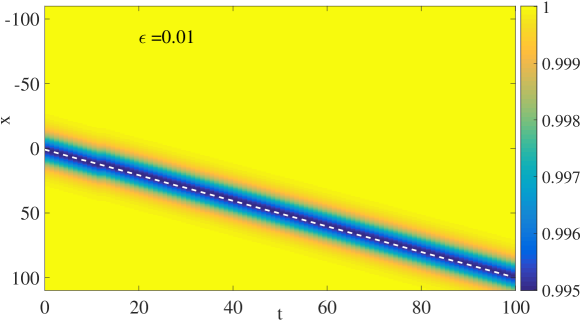
Figure 1: Propagation of the polariton wavefunction modulus, for $\epsilon=0.01$. The dashed (white) line shows the theoretical prediction of our model for the position of the soliton center (where the density is minimum), for the same initial profile.

Next, we test the validity of our approximations and analytical results by means of direct numerical simulations for the system of Eqs. (3)-(4). Our aim is to compare these results with our analytic predictions presented above. For simplicity, in our simulations, all quantities with tildes have been set equal to one, so that our initial data depend on a sole parameter, namely the small parameter $\epsilon$. Since our approach relies on a perturbation expansion, we expect results for relatively smaller values of $\epsilon$ to give a better agreement.

A series of illustrative results are shown in Figs. 1–4. In particular, Fig. 1 depicts, for $\epsilon=0.01$, the full evolution of the polariton’s wavefunction modulus. Here, it is observed that the analytical prediction for the soliton trajectory, corresponding to the dashed (red) line, closely follows the numerical result. In addition, to further verify our estimates for the soliton’s decay rate and velocity, we depict in Fig. 2 the initial (left) and final (right) profiles for $|\Psi|$ (top panels) and $n_{R}$ (bottom panels), in the same case of $\epsilon=0.01$. We also depict in the panels, shown with a dashed (red) line, the prediction of our reductive perturbation theory. For this value of the small parameter, the two are nearly indistinguishable.

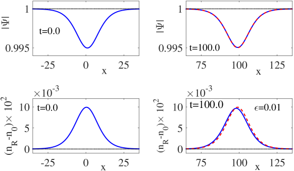
Figure 2: Initial (left panels) and final (right panels) ($t=100$) polariton wavefunction modulus (top panels) and reservoir exciton density (bottom), for $\epsilon=0.01$. The solid (blue) and dashed (red) lines show, respectively, the numerical and the theoretical predictions of our model, for the same initial profile, namely the KdV soliton.

Next, we use a relatively large value of the small parameter, namely $\epsilon=0.1$. As was to be expected, the deviations for the same duration of the propagation are more evident. First, the contour plot for this scenario, depicted in Fig. 3, shows again a fairly good agreement between our model and the numerics of the full equations, at least up to $t\approx 50$. Nevertheless, as it is shown in Fig. 4, where the initial and final (at $t=100$) snapshots for $|\Psi|$ and $n_{R}-n_{0}$ are depicted, the analytic results underestimate the speed (but only by a few percent) and overestimate the strength of the peaks (by some $15\%$).

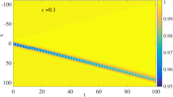
Figure 3: Same as in Fig. 1 for $\epsilon=0.1$.

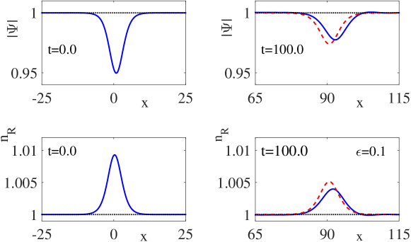
Figure 4: Same as in Fig. 2 for $\epsilon=0.1$.

For the the same case of $\epsilon=0.1$, Fig. 5 depicts the emergence and evolution of the shelf. It is clear that, in accordance to our analytical predictions based on the KdV theory, the shelf is on top of the background density, and its front propagates in the direction opposite to that of the soliton, at roughly the same speed. It is observed that the shape of the shelf becomes flatter as it propagates, and at the end of the shelf, small oscillations are clearly observed, which is the typical scenario in the KdV dynamics [41, 42, 43, 44]. Thus, the results of our simulations are in a qualitative agreement with the effective KdV picture. Nevertheless, we should note that the prediction of Eq. (38) fails to quantitatively capture the size of the shelf (the analytical estimate is about an order of magnitude larger than the numerical result), a fact that can be attributed to the asymptotic nature of the analytical prediction.

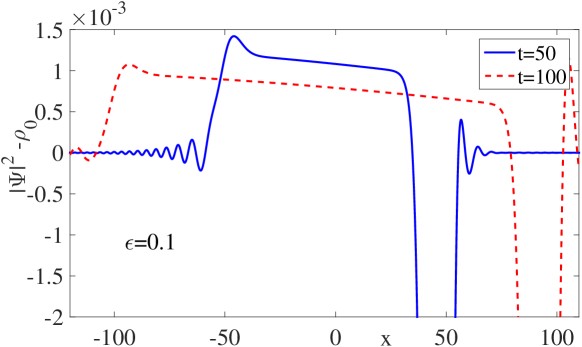
Figure 5: Linear radiation (shelf) of the polariton wavefunction modulus at $t=50$ (solid blue line) and $t=50$ (dashed red line), for $\epsilon=0.1$. The ‘dips’ of the main dark soliton pulses can be clearly observed.

As a final illustration we report the results for a scenario corresponding to physically attainable parameter values – cf., e.g., data presented in Ref. [8]. First we note that both parameters $\tilde{g}_{R}$ and $R$ are not very well known: the first is frequently set to zero, while the second can be made to vary (for instance, by playing with the size of the confinement, or width of the quantum well). Here we select values of $g_{R}=0.005\,\mathrm{meV\cdot\mu m^{2}}$ and $\hbar R=0.005\,\mathrm{meV\cdot\mu m^{2}}$, together with $g_{c}=3g_{R}=0.015\,\mathrm{meV\cdot\mu m^{2}}$, $\hbar\gamma_{R}=4\times\hbar\gamma_{C}=2\,\mathrm{meV}$. From these, and the choice $n_{C}=2\times 10^{14}\,\mathrm{m}^{-2}$, and for the case of $\epsilon=0.1$, the scaled (tilde) values are $\tilde{\alpha}=1$, $\tilde{g}_{R}=0.33$, $\tilde{\gamma}_{C}=1.67$, $\tilde{\gamma}_{R}=0.67$, and $\tilde{R}=3.33$. For these parameters, the result of the evolution of the dark soliton is shown in Fig. 6. As we can see, the agreement between the numerical evolution and the KdV approximation is again fairly good, even for this more stringent value of $\epsilon$. Notice that only the initial and final profiles are shown, but this level of agreement is maintained throughout the course of the numerical simulation.

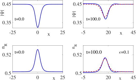
Figure 6: Same as Fig.4, but for parameters $\tilde{g}_{R}=0.33$, $\tilde{\gamma}_{C}=1.67$, $\tilde{\gamma}_{R}=0.67$, and $\tilde{R}=3.33$.

4 Conclusions

We have studied an open dissipative mean-field model for exciton-polariton condensates. In particular, the considered system is composed of a generalized open-dissipative Gross-Pitaevskii equation, describing the macroscopic wavefunction of an incoherently pumped polariton condensate, coupled to a rate equation for the exciton reservoir density. Considering a uniform pumping, and assuming that the polariton loss rate and the rate of the stimulated scattering into the condensate are sufficiently small, we have analyzed the regime of weak pumping.

Using a perturbative approach, we have derived an effective KdV equation with linear loss. This KdV model was used to describe the analytical form and the dynamics of approximate dark soliton solutions that can be supported in exciton-polariton condensates. Thus, it was found that the polariton field supports a decaying dark soliton, with a decay rate depending on the physical parameters of the problem, such as the polariton decay rate and the relative deviation of the uniform pumping from its threshold value. It was also found that the evolution of the dark soliton is accompanied by a shelf, whose emergence and subsequent dynamics are in qualitative agreement with the KdV picture. The analytical findings were found to be in fairly good agreement with the direct numerical simulations, even for the case of a relatively large value of the formal small parameter.

It would be interesting to extend our considerations to multi-dimensional and multi-component (spinor) polariton superfluid settings —see, e.g. Refs. [50, 51] and Refs. [52, 37] for work on spin dynamics of dark polariton solitons. In this setting, a quite relevant investigation would concern the existence of spinorial, vortex-free dark solitonic structures in such systems; notice that such states are known to exist in single-component Gross-Pitaevski/nonlinear Schrödinger systems, where small-amplitude dark solitonic structures obey effective Kadomtsev-Petviashvilli (KP) equations —see, e.g., the review [53] and references therein. It should also be interesting to use the methodology devised in this work to study other models that are used in the context of open dissipative systems, such as the Lugiato-Lefever equation [54] describing dissipative dynamics in optical resonators, and also supports —in the defocusing regime— dark solitons [55].

Acknowledgements. P.G.K. gratefully acknowledges the support of NSF-PHY-1602994 and of the Stavros Niarchos Foundation via the Greek Diaspora Fellowship Program. P.G.K. and A.S.R. also acknowledge the hospitality of the Synthetic Quantum Systems group and of Markus Oberthaler at the Kirchhoff Institute for Physics (KIP) at the University of Heidelberg, as well as that of the Center for Optical Quantum Technologies (ZOQ) and of Peter Schmelcher at the University of Hamburg A.S.R. acknowledges financial support from FCT throught grant UID/FIS/04650/2013. R.C.G. acknowledges support from NSF-PHY-1603058.

References

References

- [1] J. Kasprzak, M. Richard, S. Kundermann, A. Baas, P. Jeambrun, J. Keeling, F. M. Marchetti, M.H. Szymanska, R. André, J.L. Staehli, V. Savona, P. B. Littlewood, B. Deveaud, and L. S. Dang, Nature 443, 409 (2006).
- [2] R. Balili, V. Hartwell, D. Snoke, L. Pfeiffer, K. West, Science 316, 1007 (2007).
- [3] W. Lai, N. Y. Kim, S. Utsunomiya, G. Roumpos, H. Deng, M. D. Fraser, T. Byrnes, P. Recher, N. Kumada, T. Fujisawa, and Y. Yamamoto, Nature 450, 529 (2007).
- [4] H. Deng, G. S. Solomon, R. Hey, K. H. Ploog, Y. Yamamoto, Phys. Rev. Lett. 99, 126403 (2007).
- [5] H. Deng, H. Haug, and Y. Yamamoto, Rev. Mod. Phys. 82, 1489 (2010).
- [6] I. Carusotto and C. Ciuti, Rev. Mod. Phys. 85, 299 (2013).
- [7] M. Wouters and I. Carusotto, Phys. Rev. Lett. 99, 140402 (2007).
- [8] M. Wouters, I. Carusotto, and C. Ciuti, Phys. Rev. B 77, 115340 (2008).
- [9] S. Pigeon, I. Carusotto, and C. Ciuti, Phys. Rev. B 83, 144513 (2011).
- [10] J. Keeling, N.G. Berloff, Phys. Rev. Lett. 100, 250401 (2008).
- [11] M. O. Borgh, J. Keeling, and N. G. Berloff, Phys. Rev. B 81, 235302 (2010).
- [12] C. J. Pethick and H. Smith, Bose–Einstein Condensation in Dilute Gases (Cambridge University Press, Cambridge, 2002).
- [13] L. P. Pitaevskii and S. Stringari, Bose–Einstein Condensation (Oxford University Press, Oxford, 2003).
- [14] P. G. Kevrekidis, D. J. Frantzeskakis, and R. Carretero-González, The Defocusing Nonlinear Schrödinger Equation. (SIAM, Philadelphia, 2015).
- [15] P. G. Kevrekidis, D. J. Frantzeskakis, and R. Carretero-González (eds), Emergent Nonlinear Phenomena in Bose–Einstein Condensates: Theory and Experiment (Springer, Heidelberg, 2008).
- [16] R. Carretero-González, D. J. Frantzeskakis, and P. G. Kevrekidis, Nonlinearity 21, R139 (2008).
- [17] D. J. Frantzeskakis, J. Phys. A: Math. Theor. 43, 213001 (2010).
- [18] V. S. Bagnato, D. J. Frantzeskakis, P. G. Kevrekidis, B. A. Malomed, and D. Mihalache, Rom. Rep. Phys. 67, 5 (2015).
- [19] K. G. Lagoudakis, M. Wouters, M. Richard, A. Baas, I. Carusotto, R. Andre, Le Si Dang, and B. Deveaud-Plédran, Nature Phys. 4, 706 (2008).
- [20] A. Amo, S. Pigeon, D. Sanvitto, V. G. Sala, R. Hivet, I. Carusotto, F. Pisanello, G. Leménager, R. Houdré, E. Giacobino, C. Ciuti, and A. Bramati, Science 332, 1167 (2011).
- [21] G. Roumpos, M. D. Fraser, A. Löffler, S. Höfling, A. Forchel, and Y. Yamamoto, Nature Phys. 7, 129 (2011).
- [22] Lorenzo Dominici, R. Carretero-González, Jesus Cuevas-Maraver, Antonio Gianfrate, Augusto S. Rodrigues, D.J. Frantzeskakis, P.G. Kevrekidis, Giovanni Lerario, Dario Ballarini, Milena De Giorgi, Giuseppe Gigli, Daniele Sanvitto, arXiv:1706.00143.
- [23] A. Amo, S. Pigeon, D. Sanvitto,V.G. Sala, R. Hivet, I. Carusotto, F. Pisanello, G. Leménager, R. Houdreé, E. Giacobino, E Giacobino, C. Ciuti, and A. Bramati, Science 332, 1167 (2011).
- [24] G. Grosso, G. Nardin, F. Morier-Genoud, Y. Léger, and B. Deveaud-Plédran, Phys. Rev. Lett. 107, 245301 (2011).
- [25] G. Grosso, G. Nardin, F. Morier-Genoud, Y. Léger, and B. Deveaud-Plédran, Phys. Rev. B 86, 020509(R) (2012).
- [26] L. Dominici, M. Petrov, M. Matuszewski, D. Ballarini, M. De Giorgi, D. Colas, E. Cancellieri, B. Silva Fernández, A. Bramati, G. Gigli, A. Kavokin, F. Laussy, and D. Sanvitto, Nature Comm. 6, 8993 (2015).
- [27] V. Goblot, H. S. Nguyen, I. Carusotto, E. Galopin, A. Lemaître, I. Sagnes, A. Amo, and J. Bloch, Phys. Rev. Lett. 117, 217401 (2016).
- [28] X. Ma, O. A. Egorov, and S. Schumacher, Phys. Rev. Lett. 118, 157401 (2017).
- [29] Ye. Larionova, W. Stolz, and C. O. Weiss, Opt. Lett. 33, 321 (2008).
- [30] A. V. Yulin, O. A. Egorov, F. Lederer, and D. V. Skryabin Phys. Rev. A 78, 061801(R) (2008).
- [31] A. M. Kamchatnov and S. V. Korneev, J. Exp. Theor. Phys. 115, 579 (2012).
- [32] S. Komineas, S. P. Shipman, and S. Venakides, Phys. Rev. B 91, 134503 (2015).
- [33] J. Cuevas, A. S. Rodrigues, R. Carretero-González, P. G. Kevrekidis, and D. J. Frantzeskakis, Phys. Rev. B 83, 245140 (2011).
- [34] A. S. Rodrigues, P.G. Kevrekidis, R. Carretero-González, J. Cuevas, D. J. Frantzeskakis, and F. Palmero, J. Phys: Cond. Matt. 26, 15801 (2014).
- [35] L. A. Smirnov, D. A. Smirnova, E. A. Ostrovskaya, and Yu. S. Kivshar, Phys. Rev. B 89, 235310 (2014).
- [36] Y. Xue and M. Matuszewski, Phys. Rev. Lett. 112, 216401 (2014).
- [37] F. Pinsker, Annals Phys. 362, 726 (2015).
- [38] E. Wertz, L. Ferrier, D. D. Solnyshkov, R. Johne, D. Sanvitto, A. Lemaître, I. Sagnes, R. Grousson, A. V. Kavokin, P. Senellart, G. Malpuech, and J. Bloch, Nature Phys. 6, 860 (2010).
- [39] A. Jeffrey and T. Kawahara, Asymptotic Methods in Nonlinear Wave Theory (Pitman, Boston, 1982).
- [40] C. J. Knickerbocker and A. C. Newell, J. Fluid. Mech. 153, 1 (1985).
- [41] V. I. Karpman and E. M. Maslov, Zh. Eksp. Teor. Fiz. 73, 537 (1977) [Sov. Phys. JETP 46, 281 (1977)]; V. I. Karpman, Phys. Scr. 20, 462 (1979).
- [42] D. J. Kaup and A. C. Newell, Proc. R. Soc. London A 361, 413 (1978).
- [43] K. Ko and H. H. Kuehl, Phys. Rev. Lett. 40, 233 (1978).
- [44] Y. Kodama, and M. J. Ablowitz, Stud. Appl. Math. 64, 225 (1981).
- [45] Yu. S. Kivshar and B. A. Malomed, Rev. Mod. Phys. 61, 763 (1989).
- [46] M. J. Ablowitz, S. D. Dixon, T. P. Horikis, and D. J. Frantzeskakis, Proc. R. Soc. London A 467, 2597 (2011).
- [47] G. Assanto, T. R. Marchant, A. A. Minzoni, and N. F. Smyth Phys. Rev. E 84, 066602 (2011).
- [48] N. Bobrovska, E. A. Ostrovskaya, and M. Matuszewski, Phys. Rev. B 90, 205304 (2014).
- [49] M. J. Ablowitz, Nonlinear Dispersive Waves: Asymptotic Analysis and Solitons (Cambridge University Press, Cambridge, 2011).
- [50] I. A. Shelykh, Yu. G. Rubo, G. Malpuech, D. D. Solnyshkov, and A. Kavokin, Phys. Rev. Lett. 97, 066402 (2006).
- [51] M. O. Borgh, J. Keeling, and N. G. Berloff, Phys. Rev. B 81, 235302 (2010).
- [52] A. Werner, O. A. Egorov, and F. Lederer, Phys. Rev. B 85, 115315 (2012).
- [53] D. E. Pelinovsky and Yu. S. Kivshar, Phys. Rep. 331, 117 (2000).
- [54] L. A. Lugiato and R. Lefever, Phys. Rev. Lett. 58, 2209 (1987).
- [55] P. Parra-Rivas, E. Knobloch, D. Gomila, and L. Gelens, Phys. Rev. A 93, 063839 (2016).