A new class of efficient and robust energy stable schemes for gradient flows

Abstract

We propose a new numerical technique to deal with nonlinear terms in gradient flows. By introducing a scalar auxiliary variable (SAV), we construct efficient and robust energy stable schemes for a large class of gradient flows. The SAV approach is not restricted to specific forms of the nonlinear part of the free energy, and only requires to solve decoupled linear equations with constant coefficients. We use this technique to deal with several challenging applications which can not be easily handled by existing approaches, and present convincing numerical results to show that our schemes are not only much more efficient and easy to implement, but can also better capture the physical properties in these models. Based on this SAV approach, we can construct unconditionally second-order energy stable schemes; and we can easily construct even third or fourth order BDF schemes, although not unconditionally stable, which are very robust in practice. In particular, when coupled with an adaptive time stepping strategy, the SAV approach can be extremely efficient and accurate.

65M12; 35K20; 35K35; 35K55; 65Z05.

1 Introduction

Gradient flows are dynamics driven by a free energy. Many physical problems can be modeled by PDEs that take the form of gradient flows, which are often derived from the second law of thermodynamics. Examples of these problems include interface dynamics [4, 38, 42, 48, 49, 72], crystallization [24, 23, 25], thin films [34, 53], polymers [52, 30, 31, 32] and liquid crystals [45, 20, 43, 44, 29, 28, 55, 71].

A gradient flow is determined not only by the driving free energy, but also the dissipation mechanism. Given a free energy functional ${\mathcal{E}}[\phi(\bm{x})]$ bounded from below. Denote its variational derivative as $\mu=\delta{\mathcal{E}}/\delta\phi$. The general form of the gradient flow can be written as

(1.1) $$\frac{\partial\phi}{\partial t}={\mathcal{G}}\mu,$$

supplemented with suitable boundary conditions. To simplify the presentation, we assume throughout the paper that the boundary conditions are chosen such that all boundary terms will vanish when integrating by parts are performed. This is true with periodic boundary conditions or homogeneous Neumann boundary conditions.

In the above, a non-positive symmetric operator ${\mathcal{G}}$ gives the dissipation mechanism. The commonly adopted dissipation mechanisms include the $L^{2}$ gradient flow where ${\mathcal{G}}=-I$, the $H^{-1}$ gradient flow where ${\mathcal{G}}=\Delta$, or more generally non-local $H^{-\alpha}$ gradient flow where ${\mathcal{G}}=-(-\Delta)^{\alpha}$ $(0<\alpha<1)$ (cf. [1]). For more complicated dissipation mechanisms, ${\mathcal{G}}$ may be nonlinear and may depend on $\phi$. An example is the Wasserstein gradient flow for $\phi>0$, where ${\mathcal{G}}\mu=\nabla\cdot(\phi\nabla\mu)$ (cf. [20, 40]). As long as ${\mathcal{G}}$ is non-positive, the free energy is non-increasing,

(1.2) $$\frac{\mathrm{d}{\mathcal{E}}[\phi]}{\mathrm{d}t}=\frac{\delta{\mathcal{E}}}{\delta\phi}\cdot\frac{\partial\phi}{\partial t}=(\mu,{\mathcal{G}}\mu)\leq 0,$$

where $(\phi,\psi)=\int_{\Omega}\phi\psi\mathrm{d}\bm{x}$. In this paper, we will focus on the case where ${\mathcal{G}}$ is non-positive, linear and independent of $\phi$.

Although gradient flows take various forms, from the numerical perspective, a scheme is generally evaluated from the following aspects:

1. whether the scheme keeps the energy dissipation;

2. the order of its accuracy;

3. its efficiency;

4. whether the scheme is easy to implement.

Among these the first aspect is particularly important, and is crucial to eliminating numerical results that are not physical. Oftentimes, if this is not put into thorough consideration when constructing the scheme, it may require a time step extremely small to keep the energy dissipation.

Usually, the free energy functional contains a quadratic term, which we write explicitly as

(1.3) $${\mathcal{E}}[\phi]=\frac{1}{2}(\phi,{\mathcal{L}}\phi)+{\mathcal{E}}_{1}[\phi],$$

where ${\mathcal{L}}$ is a symmetric non-negative linear operator (also independent of $\phi$), and ${\mathcal{E}}_{1}[\phi]$ are nonlinear but with only lower-order derivatives than ${\mathcal{L}}$ . To obtain an energy dissipative scheme, the linear term is usually treated implicitly in some manners, while different approaches have to be used for nonlinear terms. In the next few paragraphs, we briefly review the existing approaches for dealing with the nonlinear terms.

The first approach is the convex splitting method which was perhaps first introduced in [26] but popularized by [27]. If we can express the free energy as the difference of two convex functional, namely ${\mathcal{E}}={\mathcal{E}}_{c}-{\mathcal{E}}_{e}$ where both ${\mathcal{E}}_{c}$ and ${\mathcal{E}}_{e}$ are convex about $\phi$, then a simple convex splitting scheme reads

(1.4) $$\frac{\phi^{n+1}-\phi^{n}}{\Delta t}={\mathcal{G}}\left(\frac{\delta{\mathcal{E}}_{c}}{\delta\phi}[\phi^{n+1}]-\frac{\delta{\mathcal{E}}_{e}}{\delta\phi}[\phi^{n}]\right).$$

By using the property of convex functional,

$${\mathcal{E}}_{c}[\phi_{2}]-{\mathcal{E}}_{c}[\phi_{1}]\geq\frac{\delta{\mathcal{E}}_{c}}{\delta\phi}[\phi_{1}](\phi_{2}-\phi_{1}),$$

and multiplying (1.4) with $({\delta{\mathcal{E}}_{c}}/{\delta\phi})[\phi^{n+1}]-({\delta{\mathcal{E}}_{e}}/{\delta\phi})[\phi^{n}]$, it is easy to check that the scheme satisfies the discrete energy law ${\mathcal{E}}[\phi^{n+1}]\leq{\mathcal{E}}[\phi^{n}]$ unconditionally. Because the implicit part $\delta F_{c}/\delta\phi$ is usually nonlinear about $\phi$, we need to solve nonlinear equations at each time step, which can be expensive. The scheme (1.4) is only first-order. While it is possible to construct second-order convex splitting schemes for certain situations on a case by case basis (see, for instance, [60, 8, 68]), a general formulation of second-order convex splitting schemes is not available.

The second approach is the so-called stabilization method which treats the nonlinear terms explicitly, and add a stabilization term to avoid strict time step constraint [75, 64]. More precisely, if we can find a simple linear operator $\tilde{{\mathcal{L}}}$ such that both $\tilde{{\mathcal{L}}}$ and $\tilde{{\mathcal{L}}}-(\delta^{2}{\mathcal{E}}_{1}/\delta\phi^{2})[\phi]$ are positive, then we may choose a particular convex splitting,

$${\mathcal{E}}_{c}=\frac{1}{2}(\phi,{\mathcal{L}}\phi)+\frac{1}{2}(\phi,\tilde{{\mathcal{L}}}\phi),\quad{\mathcal{E}}_{e}=\frac{1}{2}(\phi,\tilde{{\mathcal{L}}}\phi)+{\mathcal{E}}_{1}[\phi],$$

which leads to the following unconditionally energy stable scheme:

(1.5) $$\frac{\phi^{n+1}-\phi^{n}}{\Delta t}={\mathcal{G}}\left({\mathcal{L}}\phi^{n+1}+\frac{\delta{\mathcal{E}}_{1}}{\delta\phi}[\phi^{n}]+\tilde{{\mathcal{L}}}(\phi^{n+1}-\phi^{n})\right).$$

Hence, the stabilization method is in fact a special class of convex splitting method. A common choice of $\tilde{{\mathcal{L}}}$ is

$$\tilde{{\mathcal{L}}}=a_{0}+a_{1}(-\Delta)+a_{2}(-\Delta)^{2}+\ldots.$$

The advantage of the stabilization method is that when the dissipation operator ${\mathcal{G}}$ is also linear, we only need to solve a linear system like $(1-\Delta t{\mathcal{G}}({\mathcal{L}}+\tilde{{\mathcal{L}}}))\phi^{n+1}=b^{n}$ at each time step. However, it is not always the case that $\tilde{{\mathcal{L}}}$ can be found. The stabilization method can be extended to second-order schemes, but in general it can not be unconditionally energy stable, see however a recent work in [47]. On the other hand, a related method is the exponential time differencing (ETD) approach in which the operator $\tilde{{\mathcal{L}}}$ is integrated exactly (see, for instance, [41] for an example on related applications).

The third approach is the method of invariant energy quadratization (IEQ), which was proposed very recently in [70, 73]. This method is a generalization of the method of Lagrange multipliers or of auxiliary variables originally proposed in [6, 37]. In this approach, ${\mathcal{E}}_{1}$ is assumed to take the form ${\mathcal{E}}_{1}[\phi]=\int_{\Omega}g(\phi)\mathrm{d}\bm{x}$ where $g(\phi)\geq-C_{0}$ for some $C_{0}>0$. One then introduces an auxiliary variable $q=\sqrt{g+C_{0}}$, and transform (1.1) into a equivalent system,

(1.6a) $$\frac{\partial\phi}{\partial t}= {\mathcal{G}}\left({\mathcal{L}}\phi+\frac{q}{\sqrt{g(\phi)+C_{0}}}g^{\prime}(\phi)\right),$$

(1.6b) $$\frac{\partial q}{\partial t}= \frac{g^{\prime}(\phi)}{2\sqrt{g(\phi)+C_{0}}}\frac{\partial\phi}{\partial t}.$$

Using the fact that ${\mathcal{E}}_{1}[\phi]=\int_{\Omega}q^{2}\mathrm{d}\bm{x}$ is convex about $q$, we can easily construct simple and linear energy stable schemes. For instance, a first-order scheme is given by

(1.7a) $$\frac{\phi^{n+1}-\phi^{n}}{\Delta t}= {\mathcal{G}}\mu^{n+1},$$

(1.7b) $$\mu^{n+1}= {\mathcal{L}}\phi^{n+1}+\frac{q^{n+1}}{\sqrt{g(\phi^{n})+C_{0}}}g^{\prime}(\phi^{n}),$$

(1.7c) $$\frac{q^{n+1}-q^{n}}{\Delta t}= \frac{g^{\prime}(\phi^{n})}{2\sqrt{g(\phi^{n})+C_{0}}}\frac{\phi^{n+1}-\phi^{n}}{\Delta t}.$$

One can easily show that the above scheme is unconditionally energy stable. Furthermore, eliminating $q^{n+1}$ and $\mu^{n+1}$, we obtain a linear system for $\phi^{n+1}$ in the following form:

(1.8) $$\left(\frac{1}{\Delta t}-{\mathcal{G}}{\mathcal{L}}-{\mathcal{G}}\frac{(g^{\prime}(\phi^{n}))^{2}}{2g(\phi^{n})}\right)\phi^{n+1}=b^{n}.$$

Similarly, one can also construct unconditionally energy stable second-order schemes. The IEQ approach is remarkable as it allows us to construct linear, unconditionally stable, and second-order unconditionally energy stable schemes for a large class of gradient flows. However, it still suffer from the following drawbacks:

• Although one only needs to solve a linear system at each time step, the linear system usually involves variable coefficients which change at each time step.

• For gradient flows with multiple components, the IEQ approach will lead to coupled systems with variable coefficients.

• It requires that the energy density function $g(\phi)$ is bounded from below, while in some case, one can only assume that ${\mathcal{E}}_{1}[\phi]=\int_{\Omega}g(\phi)\mathrm{d}\bm{x}$ is bounded from below.

In [62], we introduced the so-called scalar auxiliary variable (SAV) approach, which inherits all advantages of IEQ approach but also overcome most of its shortcomings. More precisely, by using the Cahn-Hilliard equation and a system of Cahn-Hilliard equations as examples, we showed that the SAV approach has the following advantages:

1. For single-component gradient flows, it leads to, at each time step, linear equations with constant coefficients so it is remarkably easy to implement.

2. For multi-component gradient flows, it leads to, at each time step, decoupled linear equations with constant coefficients, one for each component.

t each time step we only need to solve a linear system of the form $(1-c_{0}\Delta t{\mathcal{G}}{\mathcal{L}})\bar{x}=\bar{b}$ twice, where $c_{0}$ is positive constant depending on the time discretization scheme. More precisely, the task for solving the gradient flow using the new SAV approach is equivalent to using an implicit scheme to solve the linear parabolic PDE: $\frac{\partial\phi}{\partial t}={\mathcal{G}}{\mathcal{L}}\phi.$ If ${\mathcal{G}}$ and ${\mathcal{L}}$ are commutative, the linear system is symmetric; even if they are not commutative, the matrix does not vary with time.

The SAV approach only requires the free energy ${\mathcal{E}}_{1}[\phi]=\int_{\Omega}g(\phi)\mathrm{d}\bm{x}$ to be bounded below, instead of a uniform lower bound for the free energy density function $g(\phi)$, enabling us to deal with a larger class of free energies.

The main goals of this paper are (i) to expand the SAV approach to a more general setting, and apply it to several challenging applications, such as non-local phase field crystals, Molecular beam epitaxial without slope section, a Q-tensor model for liquid crystals, a phase-field model for two-phase incompressible flows; (ii) to show that, besides its simplicity and efficiency, the novel schemes present better accuracy compared with other schemes; and (iii) to validate the effectiveness and robustness of the SAV approach coupled with high-order BDF schemes and adaptive time stepping.

We emphasize that the schemes are formulated in a general form that are applicable to a large class of gradient flows. We also suggest some criteria on the choice of ${\mathcal{L}}$ and ${\mathcal{E}}_{1}$, which is useful when attempting to construct numerical schemes for particular gradient flows.

The rest of paper is organized as follows. In Section 2, we describe the construction of SAV schemes for gradient flows in a general form. In Section 3, we present several numerical examples to validate the SAV approach. In Section 4, we describe how to construct higher-order SAV schemes and how to implement adaptive time stepping. We then apply the SAV approach to construct second-order unconditionally stable, decoupled linear schemes for several challenging situations in Section 5, followed by some concluding remarks in Section 6.

2 SAV approach for constructing energy stable schemes

In this section, we formulate the SAV approach introduced in [62] for a class of general gradient flows.

2.1 Gradient flows of a single function

We consdier (1.1) with free energy in the form of (1.3) such that ${\mathcal{E}}_{1}[\phi]$ is bounded from below. Without loss of generality, we assume that ${\mathcal{E}}_{1}[\phi]\geq C_{0}>0$, otherwise we may add a constant to ${\mathcal{E}}_{1}$ without altering the gradient flow. We introduce a scalar auxiliary variable $r=\sqrt{{\mathcal{E}}_{1}}$, and rewrite the gradient flow (1.1) as

(2.1a) $$\frac{\partial\phi}{\partial t}={\mathcal{G}}\mu,$$

(2.1b) $$\mu={\mathcal{L}}\phi+\frac{r}{\sqrt{{\mathcal{E}}_{1}[\phi]}}U[\phi],$$

(2.1c) $$r_{t}=\frac{1}{2\sqrt{{\mathcal{E}}_{1}[\phi]}}\int_{\Omega}U[\phi]\phi_{t}\mathrm{d}\bm{x},$$

where

(2.2) $$U[\phi]=\frac{\delta{\mathcal{E}}_{1}}{\delta\phi}.$$

Taking the inner products of the above with $\mu$, $\frac{\partial\phi}{\partial t}$ and $2r$, respectively, we obtain the energy dissipation law for (2.1):

(2.3) $$\frac{d}{dt}[(\phi,{\mathcal{L}}\phi)+r^{2}]=(\mu,{\mathcal{G}}\mu).$$

Note that this equivalent system (2.1) is similar to the system (1.6a) and (1.6b) in the IEQ approach, except that a scalar auxiliary variable $r$ is introduced instead of a function $q(\phi)$. To illustrate the advantage of SAV over IEQ, we start from a first-order scheme:

(2.4a) $$\frac{\phi^{n+1}-\phi^{n}}{\Delta t}= {\mathcal{G}}\mu^{n+1},$$

(2.4b) $$\mu^{n+1}= {\mathcal{L}}\phi^{n+1}+\frac{r^{n+1}}{\sqrt{{\mathcal{E}}_{1}[\phi^{n}]}}U[\phi^{n}],$$

(2.4c) $$\frac{r^{n+1}-r^{n}}{\Delta t}= \frac{1}{2\sqrt{{\mathcal{E}}_{1}[\phi^{n}]}}\int_{\Omega}U[\phi^{n}]\frac{\phi^{n+1}-\phi^{n}}{\Delta t}\mathrm{d}\bm{x}.$$

Multiplying the three equations with $\mu^{n+1}$, $(\phi^{n+1}-\phi^{n})/\Delta t$, $2r^{n+1}$, integrating the first two equations, and adding them together, we obtain the discrete energy law:

$$\frac{1}{\Delta t} \Big{[}\tilde{\mathcal{E}}(\phi^{n+1},r^{n+1})-\tilde{\mathcal{E}}(\phi^{n},r^{n})\big{]}$$

$$+\frac{1}{\Delta t}\Big{[}\frac{1}{2}(\phi^{n+1}-\phi^{n},{\mathcal{L}}(\phi^{n+1}-\phi^{n}))+(r^{n+1}-r^{n})^{2}\Big{]}=(\mu^{n+1},{\mathcal{G}}\mu^{n+1}),$$

where we defined a modified energy

(2.5) $$\tilde{\mathcal{E}}(\phi,r)=\frac{1}{2}(\phi,{\mathcal{L}}\phi)+r^{2}.$$

Thus, the scheme is unconditionally energy stable with the modified energy. Note that, while $r=\sqrt{{\mathcal{E}}(\phi)}$, we do not have $r^{n}=\sqrt{{\mathcal{E}}(\phi^{n})}$ so the modified energy $\tilde{\mathcal{E}}(\phi^{n},r^{n})$ is different from the original energy ${\mathcal{E}}(\phi^{n})$.

Remark 2.1.

Notice that the SAV scheme (2.4) is unconditionally energy stable (with a modified energy) for arbitrary energy splitting in (1.3) as long as ${\mathcal{E}}_{1}$ is bounded from below. One might wonder why not taking ${\mathcal{L}}=0$? Then, the scheme (2.4) would be totally explicit, i.e., without having to solve any equation, but unconditionally energy stable (with a modified energy $r^{2}(t)$)! However, energy stability alone is not sufficient for convergence. Such scheme will not be able to produce meaningful results, since the modified energy (2.5) reduces to $r^{2}(t)$ which can not control any oscillation due to derivative terms. Hence, it is necessary that ${\mathcal{L}}$ contains enough dissipative terms (with at least linearized highest derivative terms).

An important fact is that the SAV scheme (2.4) is easy to implement. ndeed, we can rewrite it as a matrix system

(2.6) $$\begin{matrix}I&-\Delta t{\mathcal{G}}&0\\ -{\mathcal{L}}&I&\frac{U[\phi^{n}]}{\sqrt{{\mathcal{E}}_{1}[\phi^{n}]}}\\ -\frac{U[\phi^{n}]}{\sqrt{{\mathcal{E}}_{1}[\phi^{n}]}}&0&I\\ \end{matrix}\begin{matrix}\phi^{n+1}\\ \mu^{n+1}\\ r^{n+1}\end{matrix}=\bar{b}^{n},$$

where $\bar{b}^{n}$ contains terms at the time step $n$. Hence, we can perform a block-Gaussian elimination to solve $r^{n+1}$ first, and then obtain $(\phi^{n+1},\mu^{n+1})$ by Indeed, taking (2.4b) and (2.4c) into (2.4a), we obtain

(2.7) $$\frac{\phi^{n+1}-\phi^{n}}{\Delta t}= {\mathcal{G}}\left[{\mathcal{L}}\phi^{n+1}+\frac{U[{\phi}^{n}]}{\sqrt{{\mathcal{E}}_{1}[{\phi}^{n}]}}\left(r^{n}+\int_{\Omega}~{}\frac{U[{\phi}^{n}]}{2\sqrt{{\mathcal{E}}_{1}[{\phi}^{n}]}}(\phi^{n+1}-\phi^{n})\mathrm{d}\bm{x}\right)\right].$$

Denote

$$b^{n}=U[{\phi}^{n}]/\sqrt{{\mathcal{E}}_{1}[{\phi}^{n}]}.$$

Then the above equation can be written as

(2.8) $$(I-\Delta t{\mathcal{G}}{\mathcal{L}})\phi^{n+1}-\frac{\Delta t}{2}{\mathcal{G}}b^{n}(b^{n},\phi^{n+1})=\phi^{n}+r^{n}{\mathcal{G}}b^{n}-\frac{\Delta t}{2}(b^{n},\phi^{n}){\mathcal{G}}b^{n}.$$

The above equation can be solved using the Sherman–Morrison–Woodbury formula [35]:

(2.9) $$(A+{U}{V}^{T})^{-1}=A^{-1}-A^{-1}{U}(I+{V}^{T}A^{-1}{U})^{-1}{V}^{T}A^{-1},$$

where $A$ is an $n\times n$ matrix, $U$ and $V$ are $n\times k$ matrices, and $I$ is the $k\times k$ identity matrix. We note that if $k\ll n$ and $A$ can be inverted efficiently, the Sherman–Morrison–Woodbury formula provides an efficient algorithm to invert the perturbed matrix $A+{U}{V}^{T}$. The system (2.8) corresponds to a case with $U$ and $V$ being $n\times 1$ vectors, so it can be efficiently solved by using (2.9). For the reader’s convenience, we write down explicitly the procedure below. Denote the righthand side of (2.8) by $c^{n}$. Multiplying (2.8) with $(I-\Delta t{\mathcal{G}}{\mathcal{L}})^{-1}$, then taking the inner product with $b^{n}$, we obtain

(2.10) $$(b^{n},\phi^{n+1})+\frac{\Delta t}{2}\gamma^{n}(b^{n},\phi^{n+1})=(b^{n},(I-\Delta t{\mathcal{G}}{\mathcal{L}})^{-1}c^{n}),$$

where $\gamma^{n}=-(b^{n},(I-\Delta t{\mathcal{G}}{\mathcal{L}})^{-1}{\mathcal{G}}b^{n})=(b^{n},(-{\mathcal{G}}^{-1}+\Delta t{\mathcal{L}})^{-1}b^{n})>0$, if we assume that ${\mathcal{G}}$ is negative definite and ${\mathcal{L}}$ is non-negative. Hence

(2.11) $$(b^{n},\phi^{n+1})=\frac{(b^{n},(I-\Delta t{\mathcal{G}}{\mathcal{L}})^{-1}c^{n})}{1+\Delta t\gamma^{n}/2}.$$

To summarize, we implement (2.4) as follows:

1. Compute $b^{n}$ and $c^{n}$ (the righthand side of (2.8));

2. Compute $(b^{n},\phi^{n+1})$ from (2.11);

3. Compute $\phi^{n+1}$ from (2.8).

Note that in (ii) and (iii) of the above procedure, we only need to solve, twice, a linear equation with constant coefficients of the form

(2.12) $$(I-\Delta t{\mathcal{G}}{\mathcal{L}})\bar{x}=\bar{b}.$$

Therefore, the above procedure is extremely efficient. In particular, if ${\mathcal{L}}=-\Delta$ and ${\mathcal{G}}=-1$ or $-\Delta$, with a tensor-product domain $\Omega$, fast solvers are available. In contrast, the convex splitting schemes usually require solving a nonlinear system, the IEQ scheme requires solving (1.8) which involves variable coefficients.

A main advantage of the SAV approach (as well as the IEQ approach) is that linear second- or even higher-order energy stable schemes can be easily constructed. We start by a semi-implicit second-order scheme based on Crank–Nicolson, which we denote as SAV/CN:

(2.13a) $$\frac{\phi^{n+1}-\phi^{n}}{\Delta t}= {\mathcal{G}}\mu^{n+1/2},$$

(2.13b) $$\mu^{n+1/2}= {\mathcal{L}}\frac{1}{2}(\phi^{n+1}+\phi^{n})+\frac{r^{n+1}+r^{n}}{2\sqrt{{\mathcal{E}}_{1}[\bar{\phi}^{n+1/2}]}}U[\bar{\phi}^{n+1/2}],$$

(2.13c) $$r^{n+1}-r^{n}= \int_{\Omega}\frac{U[\bar{\phi}^{n+1/2}]}{2\sqrt{{\mathcal{E}}_{1}[\bar{\phi}^{n+1/2}]}}(\phi^{n+1}-\phi^{n})\mathrm{d}\bm{x}.$$

In the above, $\bar{\phi}^{n+1/2}$ can be any explicit approximation of $\phi(t^{n+1/2})$ with an error of $O(\Delta t^{2})$. For instance, we may let

(2.14) $$\bar{\phi}^{n+1/2}=\frac{1}{2}(3\phi^{n}-\phi^{n-1})$$

be the extrapolation; or we can use a simple first-order scheme to obtain it, such as the semi-implicit scheme

(2.15) $$\frac{\bar{\phi}^{n+1/2}-\phi^{n}}{\Delta t/2}={\mathcal{G}}\left({\mathcal{L}}\bar{\phi}^{n+1/2}+U[\phi^{n}]\right),$$

which has a local truncation error of $O(\Delta t^{2})$.

Just as in the first-order scheme, one can eliminate $\mu^{n+1}$ and $r^{n+1}$ from the second-order schemes (2.13) to obtain a linear equation for $\phi$ similar to (2.8), so it can be solved by using the Sherman–Morrison–Woodbury formula (2.9) which only involves two linear equations with constant coefficients of the form (2.12).

Regardless of how we obtain $\bar{\phi}^{n+1/2}$, multiplying the three equations with $\mu^{n+1/2}$, $(\phi^{n+1}-\phi^{n})/\Delta t$, $(r^{n+1}+r^{n})/\Delta t$, we derive the following:

Theorem 2.1.

The scheme (2.13) is second-order accurate, unconditionally energy stable in the sense that

$$\frac{1}{\Delta t}\Big{[}\tilde{\mathcal{E}}^{n+1}-\tilde{\mathcal{E}}^{n}\Big{]}=-(\mu^{n+1/2},{\mathcal{G}}\mu^{n+1/2}),$$

where $\tilde{\mathcal{E}}$ is the modified energy defined in (2.5), and one can obtain $(\phi^{n+1},\mu^{n+1},r^{n+1})$ by solving two linear equations with constant coefficients of the form (2.12).

We can also construct semi-implicit second-order scheme based on BDF formula, which we denote as SAV/BDF:

(2.16a) $$\frac{3\phi^{n+1}-4\phi^{n}+\phi^{n-1}}{2\Delta t}= {\mathcal{G}}\mu^{n+1},$$

(2.16b) $$\mu^{n+1}= {\mathcal{L}}\phi^{n+1}+\frac{r^{n+1}}{\sqrt{{\mathcal{E}}_{1}[\bar{\phi}^{n+1}]}}U[\bar{\phi}^{n+1}],$$

(2.16c) $$3r^{n+1}-4r^{n}+r^{n-1}= \int_{\Omega}\frac{U[\bar{\phi}^{n+1}]}{2\sqrt{{\mathcal{E}}_{1}[\bar{\phi}^{n+1}]}}(3\phi^{n+1}-4\phi^{n}+\phi^{n-1})\mathrm{d}\bm{x}.$$

Here, $\bar{\phi}^{n+1}$ can be any explicit approximation of $\phi(t^{n+1})$ with an error of $O(\Delta t^{2})$. Multiplying the three equations with $\mu^{n+1}$, $(3\phi^{n+1}-4\phi^{n}+\phi^{n-1})/\Delta t$, $r^{n+1}/\Delta t$ and integrating the first two equations, and using the identity:

(2.17) $$\begin{split}2(a^{k+1},3a^{k+1}-4a^{k}+a^{k-1})=&|a^{k+1}|^{2}+|2a^{k+1}-a^{k}|^{2}+|a^{k+1}-2a^{k}+a^{k-1}|^{2}\\ &-|a^{k}|^{2}-|2a^{k}-a^{k-1}|^{2},\end{split}$$

we obtain the following:

Theorem 2.2.

The scheme (2.16) is second-order accurate, unconditionally energy stable in the sense that

$$\frac{1}{\Delta t} \Big{\{}\tilde{\mathcal{E}}[(\phi^{n+1},r^{n+1}),(\phi^{n},r^{n})]-\tilde{\mathcal{E}}[(\phi^{n},r^{n}),(\phi^{n-1},r^{n-1})]\big{\}}$$

$$+\frac{1}{\Delta t}\Big{\{}\frac{1}{4}\big{(}\phi^{n+1}-2\phi^{n}+\phi^{n-1},{\mathcal{L}}(\phi^{n+1}-2\phi^{n}+\phi^{n-1})\big{)}$$

$$+\frac{1}{2}(r^{n+1}-2r^{n}+r^{n-1})^{2}\Big{\}}=(\mu^{n+1},{\mathcal{G}}\mu^{n+1}),$$

where the modified discrete energy is defined as

$$\begin{split}\tilde{\mathcal{E}}[(\phi^{n+1},r^{n+1}),(\phi^{n},r^{n})]=&\frac{1}{4}\Big{(}(\phi^{n+1},{\mathcal{L}}\phi^{n+1})+\big{(}2\phi^{n+1}-\phi^{n},{\mathcal{L}}(2\phi^{n+1}-\phi^{n})\big{)}\Big{)}\\ &+\frac{1}{2}\big{(}(r^{n+1})^{2}+(2r^{n+1}-r^{n})^{2}\big{)},\end{split}$$

and one can obtain $(\phi^{n+1},\mu^{n+1},r^{n+1})$ by solving two linear equations with constant coefficients of the form (2.12).

We observe that the modified energy $\tilde{\mathcal{E}}[(\phi^{n+1},r^{n+1},(\phi^{n},r^{n})]$ is an approximation of the original energy ${\mathcal{E}}(\phi^{n+1})$ if $(r^{n+1})^{2}$ is an approximation of ${\mathcal{E}}_{1}(\phi^{n+1})$.

2.2 Gradient flows of multiple functions

We describe below the SAV approach for gradient flows of multiple functions $\phi_{1},\ldots,\phi_{k}$:

(2.18) $${\mathcal{E}}[\phi_{1},\ldots,\phi_{k}]=\sum_{i,j=1}^{k}d_{ij}(\phi_{i},{\mathcal{L}}\phi_{j})+{\mathcal{E}}_{1}[\phi_{1},\ldots,\phi_{k}],$$

where ${\mathcal{L}}$ is a self-adjoint non-negative linear operator, the constant matrix $A=(d_{ij})$ is symmetric positive definite. Also we assume that ${\mathcal{E}}_{1}\geq C_{1}>0$. A simple case with decoupled linear terms, i.e. $d_{ij}=\delta_{ij}$, is considered in [62]. However, some applications (cf. for example [14, 9, 21]) involve coupled linear operators which render the problem very difficult to solve numerically by existing methods.

Denote $U_{i}=\delta{\mathcal{E}}_{1}/\delta\phi_{i}$, and introduce $r(t)=\sqrt{{\mathcal{E}}_{1}}$ as the scalar auxiliary variable. With a dissipation operator ${\mathcal{G}}$ for $\phi_{i}$, the gradient flow is then given by

(2.19a) $$\frac{\partial\phi_{i}}{\partial t}= {\mathcal{G}}\mu_{i},$$

(2.19b) $$\mu_{i}= \sum_{j=1}^{k}d_{ij}{\mathcal{L}}\phi_{j}+\frac{r}{\sqrt{{\mathcal{E}}_{1}}}U_{i},$$

(2.19c) $$r_{t}= \frac{1}{2\sqrt{{\mathcal{E}}_{1}}}\int_{\Omega}U_{i}\frac{\partial\phi_{i}}{\partial t}\mathrm{d}\bm{x}.$$

Taking the inner products of the above three equations with $\mu_{i}$, $\frac{\partial\phi_{i}}{\partial t}$ and $2r$, summing over $i$ and using the facts that ${\mathcal{L}}$ is self-adjoint and $d_{ij}=d_{ji}$, we obtain the energy law:

(2.20) $$\frac{d}{dt}{\mathcal{E}}[\phi_{1},\ldots,\phi_{k}]=\sum_{i=1}^{k}({\mathcal{G}}\mu_{i},\mu_{i}).$$

Consider, for example, the following second-order SAV/CN scheme:

(2.21a) $$\frac{\phi_{i}^{n+1}-\phi_{i}^{n}}{\Delta t}= {\mathcal{G}}\mu_{i}^{n+1/2},$$

(2.21b) $$\mu_{i}^{n+1/2}= \frac{1}{2}\sum_{j=1}^{k}d_{ij}{\mathcal{L}}(\phi_{j}^{n+1}+\phi_{j}^{n})+\frac{U_{i}[{\bar{\phi}}_{1}^{n+1/2},\cdots,{\bar{\phi}}_{k}^{n+1/2}]}{2\sqrt{{\mathcal{E}}_{1}[\bar{\phi}_{1}^{n+1/2},\cdots,{\bar{\phi}}_{k}^{n+1/2}]}}(r^{n+1}+r^{n}),$$

(2.21c) $$r^{n+1}-r^{n}= \int_{\Omega}\sum_{j=1}^{k}\frac{U_{j}[\bar{\phi}_{1}^{n+1/2},\cdots,\bar{\phi}_{k}^{n+1/2}]}{2\sqrt{{\mathcal{E}}_{1}[\bar{\phi}_{1}^{n+1/2},\cdots,\bar{\phi}_{k}^{n+1/2}]}}(\phi_{j}^{n+1}-\phi_{j}^{n})\mathrm{d}\bm{x},$$

where $\bar{\phi}_{j}^{n+1/2}$ can be any second-order explicit approximation of $\phi(t^{n+1/2})$. We Multiply the above three equations with $\Delta t\mu_{i}^{n+1/2}$, $\phi_{i}^{n+1}-\phi_{i}^{n}$, $r^{n+1}+r^{n}$ and take the sum over $i$. Since ${\mathcal{L}}$ is self-adjoint and $d_{ij}=d_{ji}$, we have

$$\begin{split}\frac{1}{2}\big{(}\sum_{j=1}^{k}d_{ij}{\mathcal{L}}(\phi_{j}^{n+1}+\phi_{j}^{n}),\phi_{i}^{n+1}-\phi_{i}^{n}\big{)}=\frac{1}{2}\sum_{j=1}^{k}d_{ij}[({\mathcal{L}}\phi_{j}^{n+1},\phi_{i}^{n+1})-({\mathcal{L}}\phi_{j}^{n},\phi_{i}^{n})],\end{split}$$

which immediately leads to energy stability. Next, we describe how to implement (2.21) efficiently.

Denote

$$p_{i}^{n}=\frac{U_{i}[\bar{\phi}_{1}^{n+1/2},\cdots,\bar{\phi}_{k}^{n+1/2}]}{\sqrt{{\mathcal{E}}_{1}[\bar{\phi}_{1}^{n+1/2},\cdots,\bar{\phi}_{k}^{n+1/2}]}},$$

and substitute (2.21b) and (2.21c) into (2.21a), we can eliminate $\mu_{i}^{n+1/2}and$ $r^{n+1}$ to obtain a coupled linear system of $k$ equations of the following form

(2.22) $$\phi_{i}^{n+1}-\frac{\Delta t}{2}\sum_{j=1}^{k}d_{ij}{\mathcal{G}}{\mathcal{L}}\phi_{j}^{n+1}-\frac{1}{2}\sum_{j=1}^{k}(\phi_{j}^{n+1},p_{j}^{n}){\mathcal{G}}p_{i}^{n}=b_{i}^{n},\quad i=1,\cdots,k,$$

where $b_{i}^{n}$ includes all known terms in the previous time steps. Let us denote

(2.23) $$\begin{split}&\bar{\phi}^{n+1}=(\phi_{1}^{n+1},\cdots,\phi_{k}^{n+1})^{T},\quad\bar{b}^{n}=(b_{1}^{n},\cdots,b_{k}^{n})^{T},\\ &\bar{u}=\frac{1}{2}({\mathcal{G}}p_{1}^{n},\cdots,{\mathcal{G}}p_{k}^{n}),\quad\bar{v}=(p_{1}^{n},\cdots,p_{k}^{n}).\end{split}$$

Let us denote $D=(\frac{\Delta t}{2}d_{ij})_{i,j=1,\cdots,k}.$ The above system can be written in the following matrix form:

(2.24) $$({\cal A}+\bar{u}\bar{v}^{T})\bar{\phi}^{n+1}=\bar{b}^{n},$$

where the operator ${\cal A}$ is defined by

(2.25) $${\cal A}\bar{\phi}^{n+1}=\bar{\phi}^{n+1}-{\mathcal{G}}{\mathcal{L}}D\bar{\phi}^{n+1}.$$

Hence, by using (2.9), the solution of (2.22) can be obtained by solving two linear systems of the form ${\cal A}\bar{\phi}=\bar{b}$.

It remains to describe how to solve the linear system ${\cal A}\bar{\phi}=\bar{b}$ efficiently. Since $D$ is symmetric positive definite, we can compute an orthonormal eigen-matrix $E$ such that $D=E\Lambda E^{T}$ where $\Lambda=\text{diag}(\lambda_{1},\cdots,\lambda_{k})$. Setting $\bar{\psi}=E^{T}\bar{\phi}$, we have

$${\cal A}\bar{\phi}=\bar{\phi}-{\mathcal{G}}{\mathcal{L}}E\Lambda E^{T}\bar{\phi}=E(I-{\mathcal{G}}{\mathcal{L}}\Lambda)\bar{\psi}.$$

Hence, ${\cal A}\bar{\phi}=\bar{b}$ decouples into a sequence of elliptic equations:

(2.26) $$\psi_{i}-\lambda_{i}{\mathcal{G}}{\mathcal{L}}\psi_{i}=(E^{T}\bar{b})_{i},\quad i=1,\cdots,k.$$

To summarize, ${\cal A}\bar{\phi}=\bar{b}$ can be efficiently solved as follows:

• Compute the eigen-pair $(E,\Lambda)$;

• Compute $E^{T}\bar{b}$;

• Solve the decoupled equations (2.26);

• Finally, the solution is: $\bar{\phi}=E\bar{\psi}$.

In summary:

Theorem 2.3.

The scheme (2.21) is second-order accurate, unconditionally energy stable in the sense that

$$\begin{split}\frac{1}{2\Delta t}&\big{[}\sum_{j=1}^{k}d_{ij}({\mathcal{L}}\phi_{j}^{n+1},\phi_{i}^{n+1})+(r^{n+1})^{2}\big{]}-\frac{1}{2\Delta t}\big{[}\sum_{j=1}^{k}d_{ij}({\mathcal{L}}\phi_{j}^{n},\phi_{i}^{n})+(r^{n})^{2}\big{]}=\sum_{i=1}^{k}({\mathcal{G}}\mu_{i},\mu_{i}),\end{split}$$

and one can obtain $r^{n+1}$ and $(\phi_{j}^{n+1},\mu_{j}^{n+1})_{1\leq j\leq k}$ by solving two sequences of decoupled linear equations with constant coefficients of the form (2.26).

2.3 Full discretization

To simplify the presentation, we have only discussed the time discretization in the above. However, since the stability proofs of SAV schemes are all variational, they can be straightforwardly extended to full discrete SAV schemes with Galerkin finite element methods or Garlerkin spectral methods or even finite difference methods with summation by parts.

3 Numerical validation

In this section, we apply the SAV/CN and SAV/BDF schemes to several gradient flows to demonstrate the efficiency and accuracy of the SAV approach. In all examples, we assume periodic boundary conditions and use a Fourier-spectral method for space variables.

3.1 Allen-Cahn, Cahn-Hilliard and fractional Cahn-Hilliard equations

The Allen-Cahn [2] and Cahn-Hilliard equations [11, 12], are widely used in the study of interfacial dynamics [2, 57, 4, 38, 42, 48, 49, 72, 1]. They are built with the free energy

(3.1) $${\mathcal{E}}[\phi]=\frac{1}{2}\int\left(|\nabla\phi|^{2}+\frac{1}{4\epsilon^{2}}(1-\phi^{2})^{2}\right)\mathrm{d}\bm{x}.$$

We consider the $H^{-s}$ gradient flow, which leads to the fractional Cahn–Hilliard equation:

(3.2) $$\frac{\partial\phi}{\partial t}=-\gamma(-\Delta)^{s}(-\Delta\phi-\frac{1}{\epsilon^{2}}\phi(1-\phi^{2})),\quad 0\leq s\leq 1.$$

Here, the fractional Laplacian operator $(-\Delta)^{s}$ is defined via Fourier expansion. More precisely, if $\Omega=(0,2\pi)^{2}$, then we can express $u\in L^{2}(\Omega)$ as

$$u=\sum_{man}\hat{u}_{mn}e^{imx+iny},$$

so the fractional Laplacian is defined as

$$(-\Delta)^{s}u=\sum(m^{2}+n^{2})^{s}\hat{u}_{mn}e^{imx+iny},$$

When $s=0$ ($L^{2}$ gradient flow), (3.2) is the standard Allen–Cahn equation; when $s=1$, it becomes the standard Cahn–Hilliard equation.

To apply our schemes (2.13) or (2.16) to (3.2), we specify the operators ${\mathcal{L}}$, ${\mathcal{G}}$ and the energy ${\mathcal{E}}_{1}$ as

(3.3) $${\mathcal{L}}=-\Delta+\frac{\beta}{\epsilon^{2}},\ {\mathcal{G}}=-(-\Delta)^{s},\ {\mathcal{E}}_{1}=\frac{1}{4\epsilon^{2}}\int_{\Omega}(\phi^{2}-1-\beta)^{2}\mathrm{d}\bm{x},$$

where $\beta$ is a positive number to be chosen. Then we have

$$U[\phi]=\frac{\delta{\mathcal{E}}_{1}}{\delta\phi}=\frac{1}{\epsilon^{2}}\phi(\phi^{2}-1-\beta).$$

Example 3.1.

(Convergence rate of SAV/CN scheme for the standard Cahn-Hilliard equation) We choose the computational domain as $[0,2\pi]^{2}$, $\epsilon=0.1$, and $\gamma=1$. The initial data is chosen as smooth one $u_{0}(x,y)=0.05\sin(x)\sin(y)$.

We use the Fourier Galerkin method for spatial discretization with $N=2^{7}$, and choose $\beta=1$. To compute a reference solution, we use the fourth-order exponential time differencing Runge-Kutta method (ETDRK4) [18] with $\Delta t$ sufficiently small. The numerical errors at $t=0.032$ for SAV/CN and SAV/BDF are shown in TABLE 1, where we can observe the second-order convergence for both schemes.

Scheme		$\Delta t$=1.6e-4	$\Delta t$=8e-5	$\Delta t$=4e-5	$\Delta t$=2e-5	$\Delta t$=1e-5
SAV/CN	Error	1.74e-7	4.54e-8	1.17e-8	2.94e-9	2.01e-10
	Rate	-	1.93	1.96	1.99	2.01
SAV/BDF	Error	1.38e-6	3.72e-7	9.63e-8	2.43e-8	5.98e-9
	Rate	-	1.89	1.95	1.99	2.02

Table 1: (Example 3.1) Errors and convergence rates of SAV/CN and SAV/BDF scheme for the Cahn–Hilliard equation.

Example 3.2.

We solve a benchmark problem for the Allen–Cahn equation (see [15]). Consider a two-dimensional domain $(-128,128)^{2}$ with a circle of radius $R_{0}=100$. In other words, the initial condition is given by

(3.4) $$\phi(x,y,0)=\left\{\begin{array}[]{ll}1,&x^{2}+y^{2}<100^{2},\\ 0,&x^{2}+y^{2}\geq 100^{2}.\end{array}\right.$$

By mapping the domain to $(-1,1)^{2}$, the parameters in the Allen-Cahn equation are given by $\gamma=6.10351\times 10^{-5}$ and $\epsilon=0.0078$.

In the sharp interface limit ($\epsilon\to 0$, which is suitable because the chosen $\epsilon$ is small), the radius at the time $t$ is given by

(3.5) $$R=\sqrt{R_{0}^{2}-2t}.$$

We use the Fourier Galerkin method to express $\phi$ as

(3.6) $$\phi=\sum_{n_{1},n_{2}\leq N}\hat{\phi}_{n_{1}n_{2}}e^{i\pi(n_{1}x+n_{2}y)},$$

with $N=2^{9}$. We choose $\beta=0.1$ and let the time step $\Delta t$ vary. The computed radius $R(t)$ using the SAV/CN scheme is plotted in FIG. 1. We observe that $R(t)$ keeps monotonously decreasing and very close to the sharp interface limit value, even when we choose a relatively large $\Delta t$. In [64] this benchmark problem is solved using different stabilization methods. Our result proves to be much better than the result in that work, where the oscillation around the limit value is apparent, even if the time step has been reduced to $\Delta t=10^{-3}$. We also plot the original energy and the modified energy $(\phi^{n},{\mathcal{L}}\phi^{n})+(r^{n})^{2}$ in FIG. 1 for $\Delta t=0.5$, and find that they are very close.

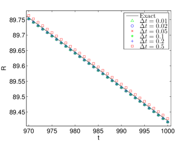
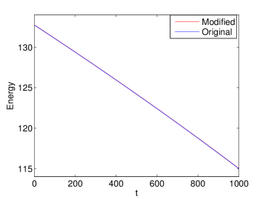
Figure 1: (Example 3.2) The evolution of radius $R(t)$ and the free energy (both original and modified). For the free energy, $\Delta t=0.5$.

Example 3.3.

(Comparison of SAV/CN and IEQ/CN schemes for the Allen–Cahn equation in 1D) The parameters are the same as the first example. The domain is chosen as $[0,2\pi]$, discretized by the finite difference method with $N=2^{10}$. The initial condition $\phi(x,0)$ is now a randomly generated function. The reference solution is also obtained using ETDRK4.

e compare the SAV/CN scheme with the IEQ/CN scheme, given as follows,

(3.7) $$\frac{\phi^{n+1}-\phi^{n}}{\Delta t}= -{\mathcal{L}}\frac{1}{2}(\phi^{n+1}+\phi^{n})+\frac{q^{n+1}+q^{n}}{2\sqrt{g(\bar{\phi}^{n+1/2})}}U[\bar{\phi}^{n+1/2}],$$

(3.8) $$q^{n+1}-q^{n}= \frac{U[\bar{\phi}^{n+1/2}]}{2\sqrt{g(\bar{\phi}^{n+1/2})}}(\phi^{n+1}-\phi^{n}).$$

We compare the result of SAV/CN and IEQ/CN schemes with the same randomly generated initial value $\phi(x,0)$ at $T=0.1$ and $T=1$. We plot the numerical results at $T=0.1$ and $T=1$ by SAV/CN and IEQ/CN schemes in FIG. 2. We used two different time steps $\Delta t=10^{-4},\ 10^{-3}$. We observe that with $\Delta t=10^{-4}$, both SAV/CN scheme and IEQ/CN scheme agree well with the reference solution. However, with $\Delta t=10^{-3}$, the solution by SAV/CN scheme still agree well with the reference solution at both $T=0.1$ and $T=1$, while the solution obtained by SAV/CN scheme has visible differences with the reference solution, and violates the maximum principle $|\phi|\leq 1$. This example clearly indicates that the SAV/CN scheme is more accurate than the IEQ/CN scheme, in addition to its easy implementation.

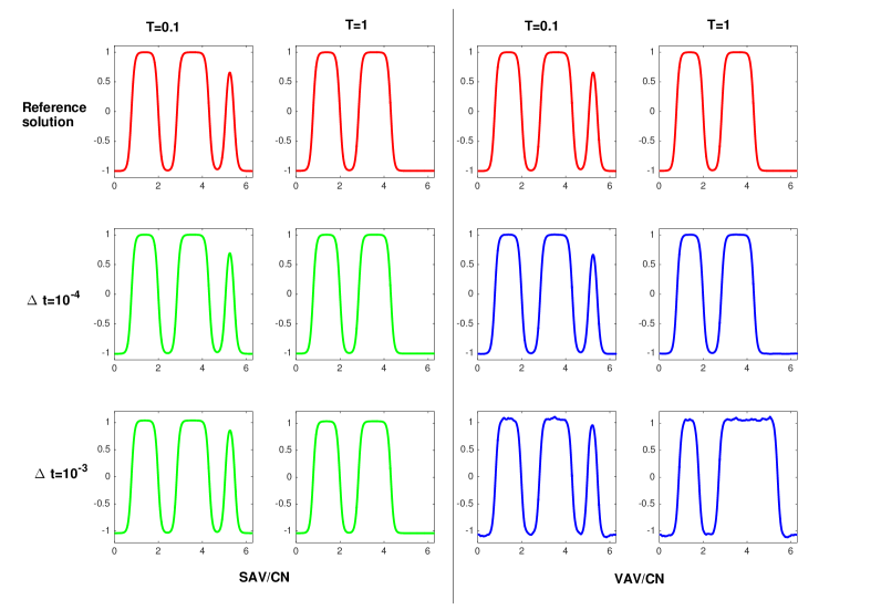
Figure 2: (Example 3.3) Comparison of SAV/CN and IEQ/CN schemes.

Example 3.4.

We examine the effect of fractional dissipation mechanism on the phase separation and coarsening process. Consider the fractional Cahn–Hilliard equation in $[0,2\pi]^{2}$. We fix $\epsilon=0.04$ and take $s$ to be $0.1$, $0.5$, $1$, respectively. We use the Fourier Galerkin method with $N=2^{7}$, and the time step $\Delta t=8\times 10^{-6}$. The initial value is the sum of a randomly generated function $\phi_{0}(x,y)$ with the average of $\phi$:

$$\bar{\phi}=\frac{1}{4\pi^{2}}\int_{0\leq x,y\leq 2\pi}\,\phi\,\mathrm{d}x\mathrm{d}y,$$

chosen as $0.25,\;0,\;-0.25$, respectively.

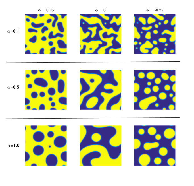
Figure 3: (Example 3.4) Configurations at time $T=0.032$ with random initial condition for different values of fractional order $\alpha$ and means $\bar{\phi}$.

We used the SAV/BDF scheme to compute the configuration at $T=0.032$, which is shown in FIG. 3. We observe that regardless of $\bar{\phi}$, when $\alpha$ is smaller, the phase separation and coarsening process is slower, which is consistent with the results in [1].

3.2 Phase field crystals

We now consider gradient flows of $\phi(\bm{x})$ that describes modulated structures. Free energy of this kind was first found in Brazovskii’s work [10], known as the Landau-Brazovskii model. Since then, the free energy, including many variants, has been adopted to study various physical systems (see for example [33, 3, 36, 69]). A usual free energy takes the form,

(3.9) $${\mathcal{E}}(\phi)=\int_{\Omega}\left\{\frac{1}{4}\phi^{4}+\frac{1-\epsilon}{2}\phi^{2}-|\nabla\phi|^{2}+\frac{1}{2}(\Delta\phi)^{2}\right\}\mathrm{d}\bm{x},$$

subjected to a constraint that the average $\bar{\phi}$ remains to be a constant. This constraint can be automatically satisfied with an $H^{-1}$ gradient flow, which is also referred to as phase field crystals model because it is widely adopted in the dynamics of crystallization [24, 23, 25]. ll the terms in the Landau–Brazovskii model come from the approximation of the virial expansion up to the fourth order. Generally, the second order term in the virial expansion is given by

$$F_{2}[\phi]=\frac{1}{2}\int_{\OmegaK}(\bm{x}-\bm{x^{\prime}})\phi(\bm{x})\phi(\bm{x^{\prime}})\mathrm{d}\bm{x}\mathrm{d}\bm{x^{\prime}}.$$

The gradient terms are obtained by approximating the kernel function $K$ in the Fourier space. The approximation involves a delta function, which actually let $K$ localized. In some recent works [du2012analysis, silling2000reformulation], the kernel $K$ is chosen as functions with a small support, which allows interactions within a small distance. Models of this kind are usually referred to as nonlocal models.

Remark. For general nonlocal models, the presence of multiple integrals (there may also be triple or quadruple integrals, etc.) will make the IEQ schemes not applicable, but does not affect the usage of SAV schemes. This is also a potential advantage of SAV over IEQ. To demonstrate the flexibility of SAV approach, we will focus on a free energy with a nonlocal kernel. Specifically, we replace the Laplacian by a nonlocal linear operator ${\mathcal{L}}_{\delta}$ [67]:

$$\mathcal{L}_{\delta}\phi(\bm{x})=\int_{\mathcal{B}(\bm{x},\delta)}\rho_{\delta}(|\bm{y}-\bm{x}|)\big{(}\phi(\bm{y})-\phi(\bm{x})\big{)}\mathrm{d}\bm{y},$$

leading to the free energy,

(3.10) $${\mathcal{E}}(\phi)=\int_{\Omega}\left\{\frac{1}{4}\phi^{4}+\frac{1-\epsilon}{2}\phi^{2}+\phi{\mathcal{L}}_{\delta}\phi+\frac{1}{2}({\mathcal{L}}_{\delta}\phi)^{2}\right\}\mathrm{d}\bm{x}.$$

Let the dissipation mechanism be given by ${\mathcal{G}}={\mathcal{L}}_{\delta}$. Then we obtain the following gradient flow,

(3.11) $$\frac{\partial\phi}{\partial t}=\mathcal{L}_{\delta}(\mathcal{L}_{\delta}^{2}\phi+2\mathcal{L}_{\delta}\phi+(1-\epsilon)\phi+\phi^{3}).$$

For the above problem, it is difficult to solve the linear system resulted from the IEQ approach, but it can be easily implemented with the SAV approach.

Let $\Omega$ be a rectangular domain $[0,2\pi)^{2}$ with periodic boundary conditions, the eigenvalues of ${\mathcal{L}}$ can be expressed explicitly. In fact, it is easy to check that for any integers $m$ and $n$, $e^{imx+iny}$ is an eigenfunction of $\mathcal{L}_{\delta}$, and the corresponding eigenvalue is given by

$$\lambda_{\delta}(m,n)=\int_{0}^{\delta}r\rho_{\delta}(r)\int_{0}^{2\pi}\left(\cos\left(r\left(m\cos\theta+n\cos\theta\right)\right)-1\right)\mathrm{d}\theta\mathrm{d}r,$$

which can be evaluated efficiently using a hybrid algorithm [22]. We choose

$$\rho_{\delta}(|\bm{x}-\bm{x^{\prime}}|)=c_{1}\frac{2(4-\alpha_{1})}{\pi}\frac{1}{\delta^{4-\alpha_{1}}r^{\alpha_{1}}}-c_{2}\frac{2(4-\alpha_{2})}{\pi}\frac{1}{\delta^{4-\alpha_{2}}r^{\alpha_{2}}},$$

with $c_{1}=20,\;c_{2}=19$, $\alpha_{1}=3,\;\alpha_{2}=0$ and $\delta=2$. Numerical results indicate that all eigenvalues are negative, which ensures the nonlocal operator ${\mathcal{L}}_{\delta}$ is negative-semidefinite.

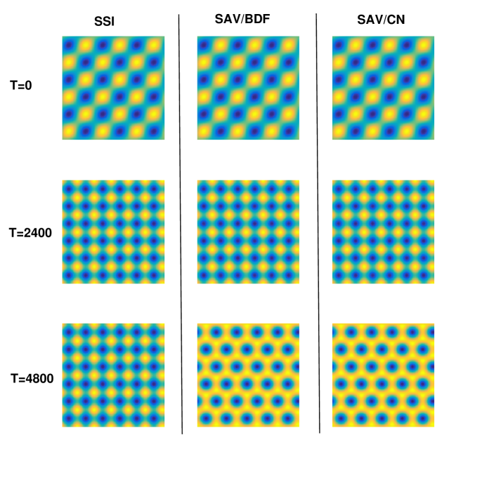
Figure 4: (Example 3.5) Configuration evolutions for NPFC models by three schemes.

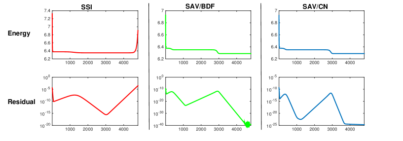
Figure 5: (Example 3.5) Energy evolutions, and residual evolutions for NPFC models by three schemes.

We applied the SAV/CN and SAV/BDF schemes to (3.11). As a comparison, we also implemented the following stabilized semi-implicit (SSI) scheme used in [17]:

$$\displaystyle\frac{\phi^{n+1}-\phi^{n}}{\Delta t} = (1-\epsilon)\mathcal{L}_{\delta}\phi^{n+1}+2\mathcal{L}_{\delta}^{2}\phi^{n+1}+\mathcal{L}_{\delta}^{3}\phi^{n+1}+(\phi^{n})^{3}$$

$$+a_{1}(1-\epsilon)\mathcal{L}_{\delta}(\phi^{n+1}-\phi^{n})-2a_{2}\mathcal{L}_{\delta}^{2}(\phi^{n+1}-\phi^{n})+a_{3}\mathcal{L}_{\delta}^{3}(\phi^{n+1}-\phi^{n}).$$

Specifically, we choose $a_{1}=0$, $a_{2}=1$ and $a_{3}=0$ which satisfy the parameters constraints provided in [17]. equation a_1¡12-3¯ϕ22(1-ϵ), a_2≥12, a_3≤12, where $\bar{\phi}$ is the volume average of $\phi$.

For the SAV schemes, we specify the linear non-negative operator as ${\mathcal{L}}=\mathcal{L}_{\delta}^{2}+2\mathcal{L}_{\delta}+I$. The time step is fixed at $\Delta t=1$.

Example 3.5.

We consider (3.11) in the two-dimensional domain $[0,50]\times[0,50]$ with periodic boundary conditions. Fix $\epsilon=0.025$ and $\bar{\phi}=0.07$. The Fourier Galerkin methods is used for spatial discretization with $N=2^{7}$.

The initial value possesses a square structure, drawn in the first row in FIG. 4, and the configurations at $T=2400$ and $4800$ are shown in the other two rows. There is no visible difference between the results for all three schemes at $T=2400$. However, for both SAV schemes, the system eventually evolves to a stable hexagonal structure, while for the SSI scheme it remains to be the unstable square structure. We also plot the free energy and residual as functions of time for the three schemes (see FIG. 5). For the SSI scheme, the residue started to increase when $T>3000$, and the free energy eventually increases, violating the energy law. On the other hand, the free energy curves for both SAV schemes remain to be dissipative, with no visible difference between them. This example clearly shows that our SAV schemes have much better stability and accuracy than the SSI scheme for the nonlocal model (3.11).

4 Higher order SAV schemes and adaptive time stepping

We describe below how to construct higher order schemes for gradient flows by combining the SAV approach with higher order BDF schemes, and how to implement adaptive time stepping to further increase the computational efficiency.

4.1 Higher order SAV schemes

For the reformulated system (2.1c)-(2.1b), we can easily use the SAV approach to construct BDF-$k$ ($k\geq 3$) schemes. Since BDF-$k$ ($k\geq 3$) schemes are not A-stable for ODEs, they will not be unconditionally stable. We will focus on BDF3 and BDF4 schemes below, as for $k>4$, the resulting BDF-$k$ schemes do not appear to be stable.

The SAV/BDF3 scheme is given by

$$\frac{11\phi^{n+1}-18\phi^{n}+9\phi^{n-1}-2\phi^{n-2}}{6\Delta t}={\mathcal{G}}\mu^{n+1},$$

$$\mu^{n+1}={\mathcal{L}}\phi^{n+1}+\frac{r^{n+1}}{\sqrt{{\mathcal{E}}_{1}[\bar{\phi}^{n+1}]}}U[\bar{\phi}^{n+1}],$$

$$11r^{n+1}-18r^{n}+9r^{n-1}-2r^{n-2}=$$

$$\int_{\Omega}\frac{U[\bar{\phi}^{n+1}]}{2\sqrt{{\mathcal{E}}_{1}[\bar{\phi}^{n+1}]}}(11\phi^{n+1}-18\phi^{n}+9\phi^{n-1}-2\phi^{n-2})\mathrm{d}\bm{x},$$

where $\bar{\phi}^{n+1}$ is a third-order explicit approximation to $\phi(t_{n+1})$. The SAV/BDF4 scheme is given by

$$\frac{25\phi^{n+1}-48\phi^{n}+36\phi^{n-1}-16\phi^{n-2}+3\phi^{n-3}}{12\Delta t}={\mathcal{G}}\mu^{n+1},$$

$$\mu^{n+1}={\mathcal{L}}\phi^{n+1}+\frac{r^{n+1}}{\sqrt{{\mathcal{E}}_{1}[\bar{\phi}^{n+1}]}}U[\bar{\phi}^{n+1}],$$

$$25r^{n+1}-48r^{n}+36r^{n-1}-16r^{n-2}+3r^{n-3}=$$

$$\int_{\Omega}\frac{U[\bar{\phi}^{n+1}]}{2\sqrt{{\mathcal{E}}_{1}[\bar{\phi}^{n+1}]}}(25\phi^{n+1}-48\phi^{n}+36\phi^{n-1}-16\phi^{n-2}+3\phi^{n-3})\mathrm{d}\bm{x},$$

where $\bar{\phi}^{n+1}$ is a fourth-order explicit approximation to $\phi(t_{n+1})$.

To obtain $\bar{\phi}^{n+1}$ in BDF3, we can use the extrapolation (BDF3A):

$$\bar{\phi}^{n+1}=3{\phi}^{n}-3{\phi}^{n-1}+{\phi}^{n-2},$$

or prediction by one BDF2 step (BDF3B):

$$\bar{\phi}^{n+1}=\text{BDF2}\{\phi^{n},{\phi}^{n-1},\Delta t\}.$$

Similarly, to get $\bar{\phi}^{n+1}$ in BDF4, we can do the extrapolation (BDF4A):

$$\bar{\phi}^{n+1}=4{\phi}^{n}-6{\phi}^{n-1}+4{\phi}^{n-2}-\phi^{n-3},$$

or prediction with one step of BDF3A (BDF4B):

$$\bar{\phi}^{n+1}=\text{BDF3}\{\phi^{n},{\phi}^{n-1},{\phi}^{n-2},\Delta t\}.$$

It is noticed that using the prediction with a lower order BDF step will double the total computation cost.

Example 4.1.

We take Cahn–Hilliard equation as an example to demonstrate the numerical performances of SAV/BDF3 and SAV/BDF4 schemes. We fix the computational domain as $[0,2\pi)^{2}$ and $\epsilon=0.1$. We use the Fourier Galerkin method for spatial discretization with $N=2^{7}$. The initial data is $u_{0}(x,y)=0.05\sin(x)\sin(y)$.

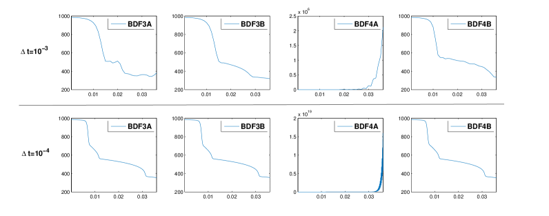
Figure 6: (Example 4.1) Energy evolutions for BDF3 and BDF4 schemes.

We first examine the energy evolution of BDF3A, BDF3B, BDF4A, and BDF4B with $\Delta t=10^{-3}$ and $\Delta t=10^{-4}$, respectively. The numerical results are shown in Fig. 6. We find that BDF4A is unstable, and BDF3A shows oscillations in energy with $\Delta t=10^{-3}$. Hence, in the following parts, we will focus on BDF3B and BDF4B, which, in what follows, are denoted in abbreviation by BDF3 and BDF4.

Then, we examine the numerical errors of BDF3 and BDF4, plotted in Fig. 7. The reference solution is obtained by ETDRK4 with a sufficiently small time step. It is observed that BDF3 and BDF4 schemes achieve the third-order and fourth-order convergence rates, respectively.

Next, we compare the numerical results of BDF2, BDF3 and BDF4. The energy evolution and the configuration at $t=0.016$ are shown in FIG. 8 (for the first row $\Delta t=10^{-3}$, and for the second row $\Delta t=10^{-4}$). We observe that at $\Delta t=10^{-4}$, all schemes lead to the correct solution although there is some visible difference in the energy evolution between BDF2 and the other higher-order schemes, but at $\Delta t=10^{-3}$, only BDF4 leads to the correct solution. The above results indicate that higher-order SAV schemes can be used to improve accuracy.

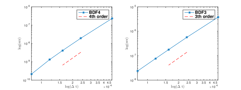
Figure 7: (Example 4.1) Numerical convergences of BDF3 and BDF4.

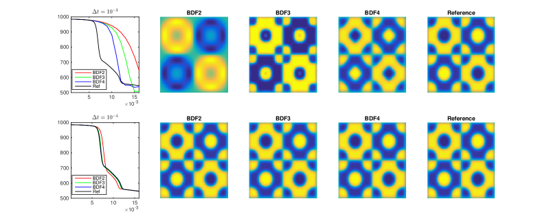
Figure 8: (Example 4.1) Comparison of BDF2, BDF3 and BDF4.

4.2 Adaptive time stepping

In many situations, the energy and solution of gradient flows can vary drastically in a certain time interval, but only slightly elsewhere. A main advantage of unconditional energy stable schemes is that they can be easily implemented with an adaptive time stepping strategy so that the time step is only dictated by accuracy rather than by stability as with conditionally stable schemes.

There are several adaptive strategies for the gradient flows. Here, we follow the adaptive time-stepping strategy in [59], which has been shown to be effective for Allen–Cahn equations. We update the time step size by using the formula

(4.3) $$A_{\!d\!p}(e,\tau)=\rho\left(\frac{tol}{e}\right)^{1/2}\tau,$$

where $\rho$ is a default safety coefficient, $tol$ is a reference tolerance, and $e$ is the relative error at each time level. In this example, we choose $\rho=0.9$ and $tol=10^{-3}$. The minimum and maximum time steps are taken as $\tau_{min}=10^{-5}$ and $\tau_{max}=10^{-2}$, respectively. The initial time step is taken as $\tau_{min}$.

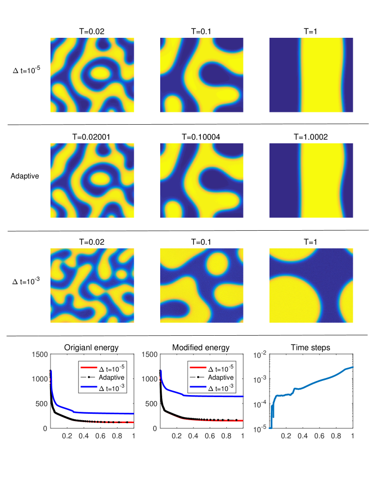
Figure 9: Example 4.2: Numerical comparisons among small time steps, adaptive time steps, and large time steps

Algorithm 1 Time step and stabilized coefficient adaptive procedure

Given: $U^{n}$, $\tau_{n}$ and stabilized parameter $S_{n}$.

  Step 1. Compute $U^{n+1}_{1}$ by the first order SAV scheme with $\tau_{n}$.

  Step 2. Compute $U^{n+1}_{2}$ by the second order SAV scheme with $\tau_{n}$.

  Step 3. Calculate $e_{n+1}=\frac{||U^{n+1}_{1}-U^{n+1}_{2}||}{||U^{n+1}_{2}||}$

  Step 4. if $e_{n+1}>tol$, then     Recalculate time step $\tau_{n}\leftarrow\max\{\tau_{min},\min\{A_{\!d\!p}(e_{n+1},\tau_{n}),\tau_{max}\}\}$.

  Step 5. goto Step 1

  Step 6. else     Update time step $\tau_{n+1}\leftarrow\max\{\tau_{min},\min\{A_{\!d\!p}(e_{n+1},\tau_{n}),\tau_{max}\}\}$.

  Step 7. endif

We take the $2$D Cahn–Hilliard equation as an example to demonstrate the performence of the time adaptivity.

Example 4.2.

Consider the $2$D Cahn–Hilliard equation on $[0,2\pi]\times[0,2\pi]$ with periodic boundary conditions and random initial data. We take $\epsilon=0.1$, and use the Fourier spectral method with $N_{x}=N_{y}=256$.

For comparison, we compute a reference solution by the SAV/CN scheme a small uniform time step $\tau=10^{-5}$ and a large uniform time step $\tau=10^{-3}$. Snapshots of phase evolutions, original energy evolutions and modified energy evolution, and the size of time steps in the adaptive experiment are shown in Fig. 9. It is observed that the adaptive-time solutions given in the middle row are in good agreement with the reference solution presented in the top row. However, the solutions with large time step are far way from the reference solution. This is also indicated by both the original energy evolutions and modified energy evolutions. Note also that the time step changes accordingly with the energy evolution. There are almost three-orders of magnitude variation in the time step, which indicates that the adaptive time stepping for the SAV schemes is very effective.

5 Various applications of the SAV approach

We emphasize that the SAV approach can be applied to a large class of gradient flows. In this section, we shall apply the SAV approach to several challenging gradient flows with different characteristics and show that the SAV approach leads to very efficient and accurate energy stable numerical schemes for these problems and those with similar characteristics.

A gradient flow with both local and non-local dissipation mechanisms Nonlocal models, such as those involving fractional Laplacian or peridynamic operators, have received much attention recently because their potential in modeling phenomena which can not be accurately described by local models. If we take the dissipation operator ${\mathcal{L}}$ in (1.1) to be a non-local dissipation operator, then the SAV approach also leads to efficient numerical schemes for non-local gradient flows.

We consider below a more complicated situation with a mixed dissipation operator ${\mathcal{L}}={\mathcal{L}}_{l}+{\mathcal{L}}_{\delta}$ where ${\mathcal{L}}_{l}$ is a local dissipation operator, and ${\mathcal{L}}_{\delta}$ is a non-local peridynamic operator [67]:

$${\mathcal{L}}_{\delta}\phi=-\int_{\Omega}\rho_{\delta}(|\bm{y}-\bm{x}|)\left(\phi(\bm{y})-\phi(\bm{x})\right)d\bm{y},$$

where $\rho_{\delta}$ is a suitable kernal function with $\delta$ being a parameter. ${\mathcal{L}}_{\delta}$ can be viewed as the variational derivative of following energy

$$E_{\delta}(\phi)=\int_{\Omega}\int_{\Omega}\rho_{\delta}(|\bm{y}-\bm{x}|)\left(\phi(\bm{y})-\phi(\bm{x})\right)^{2}d\bm{x}d\bm{y}.$$

5.1 Gradient flows with nonlocal free energy

In most gradient flows, the governing free energy is local, i.e. can be written as an integral of functions about order parameters and their derivatives on a domain $\Omega$. Actually, many of these models can be derived as approximations of density functional theory (DFT) (see for example [50]) that takes a non-local form. Recently, there have been growing interests in nonlocal models, aiming to describe phenomena that is difficult to be captured in local models. Examples include peridynamics [67] and quasicrystals [5, 7, 39].

Although more complicated forms are possible, we consider the following free energy functional that covers those in the models mentioned above,

$${\mathcal{E}}[\phi]= \int_{\Omega}\Big{(}F(\phi)+\frac{1}{2}\phi{\mathcal{L}}\phi\Big{)}\mathrm{d}\bm{x}+\frac{1}{2}\int_{\Omega}\int_{\Omega}K(|\bm{x}-\bm{x^{\prime}}|)\phi(\bm{x})\phi(\bm{x^{\prime}})\mathrm{d}\bm{x^{\prime}}\mathrm{d}\bm{x}$$

(5.1) $$:= (F(\phi),1)+\frac{1}{2}({\mathcal{L}}\phi,\phi)+\frac{1}{2}(\phi,{\mathcal{L}}_{n}\phi).$$

where ${\mathcal{L}}$ is a local symmetric positive differential operator, $K(|\bm{x}-\bm{x^{\prime}}|)$ is a kernel function, $F(\phi)$ is a nonlinear (local) free energy density, and the operator ${\mathcal{L}}_{n}$ is given by

(5.2) $$({\mathcal{L}}_{n}\phi)(\bm{x})=\int K(|\bm{x}-\bm{x^{\prime}}|)\phi(\bm{x^{\prime}})\mathrm{d}\bm{x^{\prime}}.$$

Then, the corresponding gradient flow associated with energy dissipation ${\mathcal{G}}$ is

(5.3) $$\phi_{t}={\mathcal{G}}\left({\mathcal{L}}\phi+{\mathcal{L}}_{n}\phi+f(\phi)\right),$$

where $f(\phi)=F^{\prime}(\phi)$.

ssume that $c_{1}$ and $c_{2}$ are such that the linear local part will dominate the linear nonlocal part, i.e., $c_{1}({\mathcal{L}}\phi,\phi)>c_{2}({\mathcal{L}}_{\delta}\phi,\phi)$. We can then handle the nonlocal part explicitly in the SAV approach. More precisely, we set

$${\mathcal{E}}_{l}(\phi)=\frac{c_{1}}{2}({\mathcal{L}}\phi,\phi),\quad{\mathcal{E}}_{n}(\phi)=\frac{c_{2}}{2}E_{\delta}(\phi)+(F(\phi),1).$$

Assuming${\mathcal{E}}_{n}(\phi)\geq C_{0}>0$, we introduce a scalar auxiliary variable

$$r(t)=\sqrt{{\mathcal{E}}_{n}(\phi)},$$

and rewrite the gradient flow (5.3) as

(5.4a) $$\phi_{t} ={\mathcal{G}}\left(c_{1}{\mathcal{L}}\phi+\frac{r}{\sqrt{{\mathcal{E}}_{n}(\phi)}}\left(c_{2}{\mathcal{L}}_{\delta}\phi+f(\phi)\right)\right),$$

(5.4b) $$r_{t} =\frac{1}{2\sqrt{{\mathcal{E}}_{n}(\phi)}}\left(\phi_{t},c_{2}{\mathcal{L}}_{\delta}\phi+f(\phi)\right).$$

Now we can construct the scheme based on SAV/BDF1

$$\frac{\phi^{n+1}-\phi^{n}}{\Delta t}= {\mathcal{G}}\mu^{n+1},$$

$$\mu^{n+1}= {\mathcal{L}}\phi^{n+1}+\frac{r^{n+1}}{\sqrt{{\mathcal{E}}_{n}[\phi^{n}]}}\left(c_{2}{\mathcal{L}}_{\delta}\phi^{n}+f(\phi^{n})\right),$$

$$r^{n+1}-r^{n}= \frac{1}{2\sqrt{{\mathcal{E}}_{n}[\phi^{n}]}}\Big{(}c_{2}{\mathcal{L}}_{\delta}\phi^{n}+f(\phi^{n}),\phi^{n+1}-\phi^{n}\Big{)}.$$

In general, ${\mathcal{L}}$ may not be positive and shall be controlled by the nonlinear term $F(\phi)$, as in the non-local models we mentioned above. In this case, we may put part of the non-local term together with the nonlinear term, and handle the non-local term explicitly in the SAV approach. More precisely, we split ${\mathcal{L}}_{n}={\mathcal{L}}_{n1}+{\mathcal{L}}_{n2}$ set

$${\mathcal{E}}_{l}(\phi)=\frac{1}{2}({\mathcal{L}}\phi,\phi)+\frac{1}{2}(\phi,{\mathcal{L}}_{n1}\phi),\quad{\mathcal{E}}_{n}(\phi)=\frac{1}{2}(\phi,{\mathcal{L}}_{n2}\phi)+(F(\phi),1),$$

where we assume that ${\mathcal{L}}_{n1}$ is positive and ${\mathcal{E}}_{n}(\phi)\geq C_{0}>0$. We introduce a scalar auxiliary variable

$$r(t)=\sqrt{{\mathcal{E}}_{n}(\phi)},$$

and rewrite the gradient flow (5.3) as

(5.5a) $$\phi_{t} ={\mathcal{G}}\left(({\mathcal{L}}+{\mathcal{L}}_{n1})\phi+\frac{r}{\sqrt{{\mathcal{E}}_{n}(\phi)}}\left({\mathcal{L}}_{n2}\phi+f(\phi)\right)\right),$$

(5.5b) $$r_{t} =\frac{1}{2\sqrt{{\mathcal{E}}_{n}(\phi)}}\left(\phi_{t},{\mathcal{L}}_{n2}\phi+f(\phi)\right).$$

Then the second-order BDF scheme based on SAV approach is:

(5.6a) $$\frac{3\phi^{n+1}-4\phi^{n}+\phi^{n-1}}{2\Delta t}={\mathcal{G}}\mu^{n+1},$$

(5.6b) $$\mu^{n+1}=({\mathcal{L}}+{\mathcal{L}}_{n1})\phi^{n+1}+\frac{r^{n+1}}{\sqrt{{\mathcal{E}}_{n}[\bar{\phi}^{n+1}]}}\left({\mathcal{L}}_{n2}\bar{\phi}^{n+1}+f(\bar{\phi}^{n+1})\right),$$

(5.6c) $$3r^{n+1}-4r^{n}+r^{n-1}=\frac{1}{2\sqrt{{\mathcal{E}}_{n}[\bar{\phi}^{n+1}]}}\Big{(}{\mathcal{L}}_{n2}\bar{\phi}^{n+1}+f(\bar{\phi}^{n+1}),3\phi^{n+1}-4\phi^{n}+\phi^{n-1}\Big{)}.$$

Similarly, it is easy to show that the above scheme is unconditionally energy stable, and that the scheme only requires, at each time step, solving two linear systems of the form:

(5.7) $$(I-\lambda\Delta t{\mathcal{G}}({\mathcal{L}}+{\mathcal{L}}_{n1}))\phi=f.$$

In particular, if ${\mathcal{L}}>{\mathcal{L}}_{n}$, a good choice can be ${\mathcal{L}}_{n1}=0$ and ${\mathcal{L}}_{n2}={\mathcal{L}}_{n}$, and only need to solve equations with common differential operators. Note also that the phase field crystal model considered in Subsection 3.2 is a special case with ${\mathcal{L}}=0$ and ${\mathcal{L}}_{n2}=0$.

Note that the above problem can not be easily treated with convex splitting or IEQ approaches.

5.2 Molecular beam epitaxial (MBE) without slope selection

The energy functional for molecular beam epitaxial (MBE) without slope selection is given by [46]:

(5.8) $${\mathcal{E}}(\phi)=\int_{\Omega}[-\frac{1}{2}\ln(1+|\nabla\phi|^{2})+\frac{\eta^{2}}{2}|\Delta\phi|^{2}]dx.$$

A main difficulty is that the first part of the energy density, $-\frac{1}{2}\ln(1+|\nabla\phi|^{2})$, is unbounded from below, so the IEQ approach can not be applied. However, one can show that [16] for any $\alpha_{0}>0$, there exist $C_{0}>0$ such that

(5.9) $${\mathcal{E}}_{1}(\phi)=\int_{\Omega}[-\frac{1}{2}\ln(1+|\Delta\phi|^{2})+\frac{\alpha}{2}|\Delta\phi|^{2}]dx\geq-C_{0},\quad\forall\alpha\geq\alpha_{0}>0.$$

Hence, we can choose $\alpha_{0}<\alpha<\eta^{2}$, and split ${\mathcal{E}}(\phi)$ as

$${\mathcal{E}}(\phi)={\mathcal{E}}_{1}(\phi)+\int_{\Omega}\frac{\eta^{2}-\alpha}{2}|\Delta\phi|^{2}dx.$$

Now we introduce a scalar auxiliary variable

$$r(t)=\sqrt{\int_{\Omega}\frac{\alpha}{2}|\Delta\phi|^{2}-\frac{1}{2}\log(1+|\nabla\phi|^{2})dx+C_{0}},$$

and rewrite the gradient flow for MBE as

(5.10a) $$\phi_{t}+M[(\eta^{2}-\alpha)\Delta^{2}\phi+G(\phi){r(t)}]=0,$$

(5.10b) $$r_{t}=\frac{1}{2}\int_{\Omega}G(\phi)\phi_{t}dx,$$

where

$$G(\phi)=\frac{\frac{\delta E_{1}(\phi)}{\delta\phi}}{\sqrt{\int_{\Omega}\frac{\alpha}{2}|\nabla\phi|^{2}-\frac{1}{2}\log(1+|\nabla\phi|^{2})dx+C_{0}}}.$$

Therefore, we can use the SAV approach to construct, for (5.10), second-order, linear, unconditionally energy stable schemes which only require, at each time step, solving two linear equations of the form

$$(I+\Delta t\Delta^{2})\phi=f.$$

It is clear that this above approach is much more efficient and easier to implement than existing schemes (cf., for instance, [46, 60, 56]).

5.3 Q-tensor model for rod-like liquid crystals

In many liquid crystal models, a symmetric traceless second-order tensor $Q\in\mathbb{R}^{3\times 3}$ is used to described the orientational order. We consider the Landau-de Gennes free energy [19] that has been applied to study various phenomena, both analytically (see for example [51, 54]) and numerically (see for example [66, 58, 74]). It can be written as ${\mathcal{E}}[Q(\bm{x})]={\mathcal{E}}_{b}+{\mathcal{E}}_{e}$, where

(5.11) $${\mathcal{E}}_{b} =\int_{\Omega}f_{b}(Q)\mathrm{d}\bm{x}=\int_{\Omega}[\frac{a}{2}\mbox{tr}(Q^{2})-\frac{b}{3}\mbox{tr}(Q^{3})+\frac{c}{4}(\mbox{tr}(Q^{2}))^{2}]\mathrm{d}\bm{x},$$

(5.12) $${\mathcal{E}}_{e} =\int_{\Omega}[\frac{L_{1}}{2}|\nabla Q|^{2}+\frac{L_{2}}{2}\partial_{i}Q_{ik}\partial_{j}Q_{jk}+\frac{L_{3}}{2}\partial_{i}Q_{jk}\partial_{j}Q_{ik}]\mathrm{d}\bm{x}.$$

To ensure the lower-boundedness, it requires $c>0,\;L_{1},L_{1}+L_{2}+L_{3}>0$ so that we have ${\mathcal{E}}_{b},\,{\mathcal{E}}_{e}\geq 0$.

We consider the $L^{2}$ gradient flow,

(5.13) $$\frac{\partial Q_{ij}}{\partial t}=-\frac{\delta{\mathcal{E}}}{\delta Q_{ij}},\quad 1\leq i,j\leq 3,$$

with

(5.14) $$\frac{\delta{\mathcal{E}}_{b}}{\delta Q_{ij}}= aQ_{ij}-bQ_{ik}Q_{kj}+(c+\frac{b}{3})Q_{ij}\mbox{tr}(Q)^{2},$$

(5.15) $$\frac{\delta{\mathcal{E}}_{e}}{\delta Q_{ij}}= -L_{1}\Delta Q_{ij}-\frac{L_{2}+L_{3}}{2}(\partial_{ik}Q_{jk}+\partial_{jk}Q_{ik}-\frac{2}{3}(\partial_{kl}Q_{kl})\delta_{ij}).$$

We can see that the components of $Q$ are coupled both in ${\mathcal{E}}_{b}$ and ${\mathcal{E}}_{e}$, which makes it difficult to deal with numerically.

Since we have a positive quartic term $c(\mbox{tr}Q^{2})^{2}$, we can choose $a_{1},C_{0}>0$ such that $f_{b}(Q)-a_{1}\mbox{tr}(Q^{2})/2+C_{0}>0$. We introduce a scalar auxiliary variable

$$r(t)=\sqrt{{\mathcal{E}}_{1}}:=\sqrt{{\mathcal{E}}_{b}(Q)-\int_{\Omega}\frac{a_{1}}{2}\mbox{tr}(Q^{2})\mathrm{d}\bm{x}+C_{0}}.$$

Let ${\mathcal{L}}$ be defined as

$${\mathcal{L}}Q=a_{1}Q+\frac{\delta{\mathcal{E}}_{e}}{\delta Q},$$

where $\delta{\mathcal{E}}_{e}/\delta Q:=(\delta{\mathcal{E}}_{e}/{\delta Q_{ij}})$ defines a linear operator on $Q$. Hence, we can rewrite (5.13) as:

(5.16) $$\begin{split}&\frac{\partial Q}{\partial t}=-\mu,\\ &\mu={\mathcal{L}}Q+\frac{r(t)}{\sqrt{{\mathcal{E}}_{1}}}\frac{\delta{\mathcal{E}}_{1}}{\delta Q};\\ &r_{t}=\frac{1}{2\sqrt{{\mathcal{E}}_{1}}}\int_{\Omega}\frac{\delta{\mathcal{E}}_{1}}{\delta Q}:Q_{t}\mathrm{d}\bm{x}.\end{split}$$

Then, the SAV/CN scheme for (5.16) is:

(5.17a) $$\frac{Q^{n+1}-Q^{n}}{\Delta t}= -\mu^{n+1/2},$$

(5.17b) $$\mu^{n+1/2}= {\mathcal{L}}\frac{1}{2}(Q^{n+1}+Q^{n})+\frac{r^{n+1}+r^{n}}{2\sqrt{{\mathcal{E}}_{1}[\bar{Q}^{n+1/2}]}}\frac{\delta{\mathcal{E}}_{1}}{\delta Q}[\bar{Q}^{n+1/2}],$$

(5.17c) $$r^{n+1}-r^{n}= \int_{\Omega}\frac{1}{2\sqrt{{\mathcal{E}}_{1}[\bar{Q}^{n+1/2}]}}\left(\frac{\delta{\mathcal{E}}_{1}}{\delta Q}[\bar{Q}^{n+1/2}]\right)_{ij}(Q_{ij}^{n+1}-Q_{ij}^{n})\mathrm{d}\bm{x}.$$

One can easily show that the above scheme is unconditionally energy stable. Below, we describe how to implement it efficiently.

Denoting

$$S_{ij}=\frac{1}{2\sqrt{{\mathcal{E}}_{1}[\bar{Q}^{n+1/2}]}}\left(\frac{\delta{\mathcal{E}}_{1}}{\delta Q}[\bar{Q}^{n+1/2}]\right)_{ij},\quad S=(S_{ij}),$$

we can rewrite (5.17) into a coupled linear system of the form

(5.18) $$(1+\lambda{\mathcal{L}})Q_{ij}^{n+1}+S_{ij}\alpha^{n+1}=b_{ij}^{n},\quad 1\leq i,j\leq 3,$$

where $\lambda=\frac{\Delta t}{2}$, and the scalar $\alpha^{n+1}=\sum_{k,l}(S_{kl},Q_{kl}^{n+1})$ can be solved explicitly as follows. Multiplying (5.18) with $(1+\lambda{\mathcal{L}})^{-1}$, we get

(5.19) $$Q_{ij}^{n+1}+\alpha^{n+1}\big{(}(I+\lambda{\mathcal{L}})^{-1}S\big{)}_{ij}=\Big{(}(1+\lambda{\mathcal{L}})^{-1}b^{n}\Big{)}_{ij},\quad 1\leq i,j\leq 3.$$

Then taking the inner product of the above with $S$, we obtain

(5.20) $$\alpha^{n+1}\bigg{(}1+\sum_{i,j}\Big{(}S_{ij},\big{(}(1+\lambda{\mathcal{L}})^{-1}S\big{)}_{ij}\Big{)}\bigg{)}=\sum_{i,j}\Big{(}(I+\lambda{\mathcal{L}})^{-1}b^{n}\Big{)}_{ij}.$$

Thus, we can find $\alpha^{n+1}$ by solving, for each $i,j$, two equations of the form

(5.21) $$(I+\lambda{\mathcal{L}})Q_{ij}=g_{ij},$$

which can be efficiently solved since they are simply coupled second-order equations with constant coefficients. For example, in the case of periodic boundary conditions, we can write down the solution explicitly as follows. Because $Q$ is symmetric and traceless, we choose $\bm{x}=(Q_{11},Q_{22},Q_{12},Q_{13},Q_{23})^{T}$ as independent variables. We expand the above five variables by Fourier series,

$$Q_{ij}=\sum_{k_{1},k_{2},k_{3}}\hat{Q}_{ij}^{k_{1}k_{2}k_{3}}\exp(i(k_{1}x_{1}+k_{2}x_{2}+k_{3}x_{3})).$$

Then, when solving the linear equation (5.21), only the Fourier coefficients with the same indices $(k_{1},k_{2},k_{3})$ are coupled. More precisely, for each $(k_{1},k_{2},k_{3})$, and the coefficient matrix for the unknowns $\hat{Q}_{ij}^{k_{1}k_{2}k_{3}}$ with $(ij=11,22,12,13,23)$ is given by

$$A_{k_{1}k_{2}k_{3}}=1+\lambda(a_{1}+L_{1}(k_{1}^{2}+k_{2}^{2}+k_{3}^{2}))I$$

$$-\lambda\frac{L_{2}+L_{3}}{2}\left(\begin{array}[]{ccccc}-\frac{2}{3}k_{1}^{2}-\frac{1}{3}k_{3}^{2}&\frac{1}{3}k_{2}^{2}-\frac{1}{3}k_{3}^{2}&-\frac{1}{3}k_{1}k_{2}&-\frac{1}{3}k_{1}k_{3}&\frac{2}{3}k_{2}k_{3}\\ \frac{1}{3}k_{1}^{2}-\frac{1}{3}k_{3}^{2}&-\frac{2}{3}k_{2}^{2}-\frac{1}{3}k_{3}^{2}&-\frac{1}{3}k_{1}k_{2}&\frac{2}{3}k_{1}k_{3}&-\frac{1}{3}k_{2}k_{3}\\ -\frac{1}{2}k_{1}k_{2}&-\frac{1}{2}k_{1}k_{2}&-\frac{1}{2}k_{1}^{2}-\frac{1}{2}k_{2}^{2}&-\frac{1}{2}k_{2}k_{3}&-\frac{1}{2}k_{1}k_{3}\\ 0&\frac{1}{2}k_{1}k_{3}&-\frac{1}{2}k_{2}k_{3}&-\frac{1}{2}k_{1}^{2}-\frac{1}{2}k_{3}^{2}&-\frac{1}{2}k_{1}k_{2}\\ \frac{1}{2}k_{2}k_{3}&0&-\frac{1}{2}k_{1}k_{3}&-\frac{1}{2}k_{1}k_{2}&-\frac{1}{2}k_{2}^{2}-\frac{1}{2}k_{3}^{2}\end{array}\right).$$

Hence, we can obtain the Fourier coefficients $\hat{Q}_{ij}^{k_{1}k_{2}k_{3}}$, for each $i,\,j$, by inverting the above $5\times 5$ matrix.

5.4 Phase-field model of two phase incompressible flows

We consider here a phase-field model for the mixture of two incompressible, immiscible fluids [65]. Let $\phi$ be a labeling function to identify the two fluids, i.e.,

(5.22) $$\phi({x},t)=\begin{cases}\hskip 8.0pt1\quad{x}\in\text{in fluid 1},\\ -1\quad{x}\in\text{in fluid 2},\end{cases}$$

with a smooth interfacial layer of thickness $\eta$. Consider a mixing free energy

$$E_{mix}(\phi)=\lambda\int_{\Omega}(\frac{1}{2}|\nabla\phi|^{2}+F(\phi))\,\mathrm{d}\bm{x}=\lambda\int_{\Omega}\frac{1}{2}|\nabla\phi|^{2}\,\mathrm{d}\bm{x}+E_{1}(\phi),$$

with $F(\phi)=\frac{1}{4\eta^{2}}(\phi^{2}-1)^{2}$. For the sake of simplicity, we consider the two fluids having the same density $\rho_{0}$. Then, the Navier-Stokes Cahn-Hilliard phase field model for the two-phase incompressible flow is as follows (cf., for instance, [4, 48]):

(5.23) $$\phi_{t}+(u\cdot\nabla)\phi=\nabla\cdot(\gamma\nabla\mu),$$

(5.24) $$\mu=\frac{\delta E_{mix}}{\delta\phi}=-\lambda\Delta\phi+\lambda F^{\prime}(\phi);$$

and

(5.25) $$\rho_{0}(u_{t}+(u\cdot\nabla)u)=\nu\Delta u-\nabla p+\mu\nabla\phi;$$

and

(5.26) $$\nabla\cdot u=0;$$

subject to suitable boundary conditions for $\phi,\mu,u$. In the above, $\lambda$ is a mixing coefficient, $\gamma$ is a relaxation coefficients and $\nu$ is the viscosity coefficient; the unknown are $\phi,\mu,u,p$ with $u$ being the velocity and $p$ the pressure. Taking the inner product of (5.23), (5.24) and (5.25) with $\mu$, $\phi_{t}$ and $u$, respectively, we obtain the following energy dissipation law:

$$\frac{\mathrm{d}}{\mathrm{d}t}\int_{\Omega}\{\frac{\rho_{0}}{2}\mathrm{d}\bm{x}\,|u|^{2}+\frac{\lambda}{2}|\nabla\phi|^{2}+{\lambda}F(\phi)\}=-\int_{\Omega}\{\nu|\nabla u|^{2}+\gamma|\nabla\mu|^{2}\}.$$

To apply the SAV approach, we introduce $r(t)=\sqrt{E_{1}(\phi)+\delta}$, and replace (5.24) by

(5.27) $$\begin{split}&\mu=-\lambda\Delta\phi+\lambda\frac{r(t)}{\sqrt{E_{1}(\phi)+\delta}}F^{\prime}(\phi),\\ &r_{t}=\frac{1}{2\sqrt{E_{1}(\phi)+\delta}}\int_{\Omega}F^{\prime}(\phi)\,\phi_{t}\mathrm{d}\bm{x}.\end{split}$$

Let us denote $\bar{\phi}^{n+1}:=2\phi^{n}-\phi^{n-1}$ and $\bar{u}^{n+1}:=2u^{n}-u^{n-1}$. Then, we can modify the scheme (3.9) in [63] to construct the SAV/BDF2 scheme for (5.23)-(5.27)-(5.25)-(5.26):

(5.28) $$\begin{split}&\frac{3\phi^{n+1}-4\phi^{n}+\phi^{n-1}}{2\Delta t}+\hat{u}^{n+1}\cdot\nabla\bar{\phi}^{n+1}=\gamma\Delta\mu^{n+1},\\ &\mu^{n+1}=-\lambda\Delta\phi^{n+1}+\frac{\lambda r^{n+1}}{\sqrt{E_{1}[\bar{\phi}^{n+1}]+\delta}}F^{\prime}(\bar{\phi}^{n+1}),\\ &\frac{3r^{n+1}-4r^{n}-r^{n-1}}{2\Delta t}=\int_{\Omega}\frac{F^{\prime}(\bar{\phi}^{n+1})}{2\sqrt{E_{1}[\bar{\phi}^{n+1}]+\delta}}\frac{3\phi^{n+1}-4\phi^{n}+\phi^{n-1}}{2\Delta t}\,dx,\end{split}$$

where $\hat{u}^{n+1}=\tilde{u}^{n+1}$ or $\hat{u}^{n+1}=2u^{n}-u^{n-1}$;

(5.29) $$\begin{split}&\rho_{0}\{\frac{3\tilde{u}^{n+1}-4u^{n}+u^{n-1}}{2\Delta t}+\bar{u}^{n+1}\cdot\nabla\tilde{u}^{n+1}\}\\ &\hskip 36.135pt-\nu\Delta\tilde{u}^{n+1}+\nabla p^{n}-\mu^{n+1}\nabla\bar{\phi}^{n+1}=0;\end{split}$$

(5.30) $$\begin{split}&\Delta(p^{n+1}-p^{n})=\frac{3\rho_{0}}{2\Delta t}\nabla\cdot\tilde{u}^{n+1},\quad\partial_{n}(p^{n+1}-p^{n})|_{\partial\Omega}=0;\\ &u^{n+1}=\tilde{u}^{n+1}-\frac{2\Delta t}{3\rho_{0}}\nabla(p^{n+1}-p^{n}).\end{split}$$

Several remarks are in order:

• The pressure is decoupled from the rest by a pressure-correction projection method; $r^{n+1}$ can be eliminated from (5.28).

• If we take $\hat{u}^{n+1}=\tilde{u}^{n+1}$, one can show, similarly as in [63], that the scheme is unconditionally stable, linear and second-order, but weakly coupled between $(\phi^{n+1},w^{n+1},\tilde{u}^{n+1})$ by the term $\tilde{u}^{n+1}\cdot\nabla\bar{\phi}^{n+1}$. It is easy to see that the weakly coupled linear system is positive definite.

• On the other hand, if we take $\hat{u}^{n+1}=2u^{n}-u^{n-1}$, the scheme is linear, decoupled and second-order, only requires solving a sequence of Poisson type equations at each time step, but not unconditionally energy stable.

• One can use the decoupled scheme with $\hat{u}^{n+1}=2u^{n}-u^{n-1}$ as a preconditioner for the coupled scheme with $\hat{u}^{n+1}=\tilde{u}^{n+1}$.

Error estimate Generally speaking, the energy dissipation itself does not guarantee the convergence. So it is important to establish, at least for a representative class of problems, that the numerical solution by the SAV schemes will converge, with an error estimate, to the exact solution of the original problem. In this section, we shall prove such a result. We shall only consider the SAV/CN scheme. Similar results hold for the SAV/BDF scheme.

In what follows, we assume that the dissipation operator ${\mathcal{G}}$ is linear and denote

$$G(u)=(u,-{\mathcal{G}}u),\ L(u)=(u,{\mathcal{L}}u).$$

Theorem 5.1.

Let $\phi$ be the solution of (1.1) with the free energy (1.3) satisfying ${\mathcal{E}}_{1}[\phi]\geq C_{0}>0$. We assume $\phi$, ${\mathcal{L}}\phi$, ${\mathcal{G}}\phi$, ${\mathcal{G}}{\mathcal{L}}\phi\in C^{3}([0,T];L^{2})$, ${\mathcal{E}}[\phi(t)]\in C^{3}([0,T])$, and

$$||U[\phi]||^{2},\ ||U[\big{(}3\phi(t^{n})-\phi(t^{n-1})\big{)}/2]||^{2},\ G(U[\phi]),$$

$$G\Big{(}U[\big{(}3\phi(t^{n})-\phi(t^{n-1})\big{)}/2]\Big{)}\leq C_{1},$$

where $U[\phi]=\frac{\delta{\mathcal{E}}_{1}}{\delta\phi}$. Denote $M={\mathcal{E}}[\phi(0)]$, an upper bound of both ${\mathcal{E}}[\phi(t)]$ and ${\mathcal{E}}[\phi^{n}]$. We further assume there exist positive constants $C_{2}(M),\ C_{3}(M),\ C_{4}$ such that:

1. For any $\phi_{1},\phi_{2}$ satisfying ${\mathcal{E}}[\phi_{1}],{\mathcal{E}}[\phi_{2}]\leq M$, we have ${\mathcal{E}}[(3\phi_{1}-\phi_{2})/2]\leq C_{2}(M)$.

2. For any $\phi_{1},\phi_{2}$ satisfying ${\mathcal{E}}[\phi_{1}],{\mathcal{E}}[\phi_{2}]\leq C_{2}(M)$, we have $|{\mathcal{E}}_{1}[\phi_{1}]-{\mathcal{E}}_{1}[\phi_{2}]|^{2}\leq C_{3}(M)L\big{(}\phi_{2}-\phi_{1}\big{)}$.

3. $||U[\phi_{2}]-U[\phi_{1}]||^{2},\ G\big{(}U[\phi_{2}]-U[\phi_{1}]\big{)}\leq C_{4}L\big{(}\phi_{2}-\phi_{1}\big{)}$.

Then, the numerical solution of the SAV/CN scheme (2.13a)-(2.13c), satisfies the following estimate:

(5.31) $$L\Big{(}\phi^{n}-\phi(t^{n})\Big{)}+\big{(}r^{n}-r(t^{n})\big{)}^{2}\leq C\exp\Big{(}(1-C\Delta t)^{-1}t^{n}\Big{)}\Delta t^{4}.$$

Proof 5.2.

Denote the errors as $e^{n}=\phi^{n}-\phi(t^{n})$, $s^{n}=r^{n}-r(t^{n})$ and $w^{n+1/2}=\mu^{n+1/2}-\mu(t^{n+1/2})$. By comparing to the PDE at $t^{n+1/2}$, the equations for the errors are written as

(5.32) $$\frac{e^{n+1}-e^{n}}{\Delta t}= {\mathcal{G}}w^{n+1/2}+T_{1}^{n}$$

$$w^{n+1/2}= \frac{1}{2}{\mathcal{L}}(e^{n+1}+e^{n})+\frac{s^{n+1}+s^{n}}{2\sqrt{{\mathcal{E}}_{1}[\bar{\phi}^{n+1/2}]}}U[\bar{\phi}^{n+1/2}]$$

(5.33) $$+\frac{r(t^{n+1})+r(t^{n})}{2}\Big{(}\frac{U[\bar{\phi}^{n+1/2}]}{\sqrt{{\mathcal{E}}_{1}[\bar{\phi}^{n+1/2}]}}-\frac{U[(3\phi(t^{n})-\phi(t^{n-1}))/2]}{\sqrt{{\mathcal{E}}_{1}[(3\phi(t^{n})-\phi(t^{n-1}))/2]}}\Big{)}+T^{n},$$

$$s^{n+1}-s^{n}= \int\mathrm{d}\bm{x}\frac{U[\bar{\phi}^{n+1/2}]}{2\sqrt{{\mathcal{E}}_{1}[\bar{\phi}^{n+1/2}]}}(e^{n+1}-e^{n})$$

(5.34) $$+\Big{(}\frac{U[\bar{\phi}^{n+1/2}]}{2\sqrt{{\mathcal{E}}_{1}[\bar{\phi}^{n+1/2}]}}-\frac{U[(3\phi(t^{n})-\phi(t^{n-1}))/2]}{2\sqrt{{\mathcal{E}}_{1}[(3\phi(t^{n})-\phi(t^{n-1}))/2]}}\Big{)}(\phi(t^{n+1})-\phi(t^{n}))+v^{n},$$

where $T^{n}=T^{n}_{2}+T^{n}_{3}+T^{n}_{4}$ and $v^{n}=v^{n}_{1}+v^{n}_{2}+v^{n}_{3}$ with

$$T^{n}_{1}= \frac{1}{\Delta t}(\phi(t^{n+1})-\phi(t^{n}))-\phi_{t}(t^{n+1/2}),$$

$$T^{n}_{2}= \frac{1}{2}{\mathcal{L}}(\phi(t^{n+1})+\phi(t^{n})-2\phi(t^{n+1/2})),$$

$$T^{n}_{3}= \frac{r(t^{n+1})+r(t^{n})}{2}\Big{(}\frac{U[(3\phi(t^{n})-\phi(t^{n-1}))/2]}{\sqrt{{\mathcal{E}}_{1}[(3\phi(t^{n})-\phi(t^{n-1}))/2]}}-\frac{U[\phi(t^{n+1/2})]}{r(t^{n+1/2})}\Big{)},$$

$$T^{n}_{4}= \frac{1}{2}(r(t^{n+1})+r(t^{n})-2r(t^{n+1/2}))\frac{U[\phi(t^{n+1/2})]}{2r(t^{n+1/2})},$$

$$v^{n}_{1}= r(t^{n+1})-r(t^{n})-\Delta tr_{t}(t^{n+1/2}),$$

$$v^{n}_{2}= (\phi(t^{n+1})-\phi(t^{n}))\Big{(}\frac{U[(3\phi(t^{n})-\phi(t^{n-1}))/2]}{\sqrt{{\mathcal{E}}_{1}[(3\phi(t^{n})-\phi(t^{n-1}))/2]}}-\frac{U[\phi(t^{n+1/2})]}{r(t^{n+1/2})}\Big{)},$$

$$v^{n}_{3}= \frac{U[\phi(t^{n+1/2})]}{2r(t^{n+1/2})}(\phi(t^{n+1})-\phi(t^{n})-\Delta t\phi_{t}(t^{n+1/2})).$$

$T^{n}$ and $v^{n}$ are truncation errors that we will write down later. Multiplying (5.32) with $w^{n+1/2}$, (5.33) with $e^{n+1}-e^{n}$, and (5.34) with $s^{n+1}+s^{n}$, then summing up three equalities, we get

$$\frac{1}{2}\big{(}(e^{n+1},{\mathcal{L}}e^{n+1})-(e^{n},{\mathcal{L}}e^{n})\big{)}+(s^{n+1})^{2}-(s^{n})^{2}+\Delta tG(w^{n+1/2})$$

$$= -\frac{r(t^{n+1})+r(t^{n})}{2}\Delta t\left({\mathcal{G}}w^{n+1/2},\frac{U[\bar{\phi}^{n+1/2}]}{\sqrt{{\mathcal{E}}_{1}[\bar{\phi}^{n+1/2}]}}-\frac{U[(3\phi(t^{n})-\phi(t^{n-1}))/2]}{\sqrt{{\mathcal{E}}_{1}[(3\phi(t^{n})-\phi(t^{n-1}))/2]}}\right)$$

$$+(s^{n+1}+s^{n})\left(\phi(t^{n+1})-\phi(t^{n}),\frac{U[\bar{\phi}^{n+1/2}]}{\sqrt{{\mathcal{E}}_{1}[\bar{\phi}^{n+1/2}]}}-\frac{U[(3\phi(t^{n})-\phi(t^{n-1}))/2]}{\sqrt{{\mathcal{E}}_{1}[(3\phi(t^{n})-\phi(t^{n-1}))/2]}}\right)$$

$$+(w^{n+1/2},T_{1}^{n})+\Delta t({\mathcal{G}}w^{n+1/2},T^{n})+(s^{n+1}+s^{n})v^{n}$$

In the above, we substitute several $e^{n+1}-e^{n}$ with $\Delta t{\mathcal{G}}w^{n+1/2}$.

First, we estimate the terms relevant to the difference

$$\frac{U[a]}{\sqrt{{\mathcal{E}}_{1}[a]}}-\frac{U[b]}{\sqrt{{\mathcal{E}}_{1}[b]}}=U[a]\frac{{\mathcal{E}}_{1}[a]-{\mathcal{E}}_{1}[b]}{\sqrt{{\mathcal{E}}_{1}[a]{\mathcal{E}}_{1}[b]({\mathcal{E}}_{1}[a]+{\mathcal{E}}_{1}[b])}}+\frac{U[a]-U[b]}{\sqrt{{\mathcal{E}}_{1}[b]}}=A_{1}+A_{2}.$$

We have

$$G(A_{1}+A_{2})\leq 2G(A_{1})+2G(A_{2})$$

$$\leq \frac{1}{C_{0}^{3}}G(U[a])|{\mathcal{E}}_{1}[a]-{\mathcal{E}}_{1}[b]|^{2}+\frac{2}{C_{0}}G(U[a]-U[b])$$

$$\leq \frac{1}{C_{0}^{3}}G(U[a])|{\mathcal{E}}_{1}[a]-{\mathcal{E}}_{1}[b]|^{2}+\frac{2C_{4}}{C_{0}}L(a-b).$$

Let $a=\big{(}3\phi(t^{n})-\phi(t^{n-1})\big{)}/2$ and $b=\bar{\phi}^{n+1/2}$. Together with the condition (ii), we obtain

$$G\left(\frac{U[\bar{\phi}^{n+1/2}]}{\sqrt{{\mathcal{E}}_{1}[\bar{\phi}^{n+1/2}]}}-\frac{U[(3\phi(t^{n})-\phi(t^{n-1}))/2]}{\sqrt{{\mathcal{E}}_{1}[(3\phi(t^{n})-\phi(t^{n-1}))/2]}}\right)$$

$$\leq \frac{1}{C_{0}^{3}}C_{1}C_{3}(M)L\left(\frac{3}{2}e^{n}-\frac{1}{2}e^{n-1}\right)+\frac{2C_{4}}{C_{0}}L\left(\frac{3}{2}e^{n}-\frac{1}{2}e^{n-1}\right)$$

$$\leq C_{5}\big{(}L(e^{n})+L(e^{n-1})\big{)}.$$

Then, keep $a$ unchanged and let $b=\phi(t^{n+1/2})$, we have

$$G\left(\frac{U[\phi(t^{n+1/2})]}{r(t^{n+1/2})}-\frac{U[(3\phi(t^{n})-\phi(t^{n-1}))/2]}{\sqrt{{\mathcal{E}}_{1}[(3\phi(t^{n})-\phi(t^{n-1}))/2]}}\right)$$

$$\leq \left(\frac{1}{C_{0}^{3}}C_{1}C_{3}(M)+\frac{2C_{4}}{C_{0}}\right)L\left(\frac{3}{2}\phi(t^{n})-\frac{1}{2}\phi(t^{n-1})-\phi(t^{n+1/2})\right)$$

$$\leq C_{6}\Delta t^{4}\big{(}||\phi_{tt}||^{2}+||({\mathcal{L}}\phi)_{tt}||^{2}\big{)}.$$

Similarly, we also have

$$\left|\left|\frac{U[\bar{\phi}^{n+1/2}]}{\sqrt{{\mathcal{E}}_{1}[\bar{\phi}^{n+1/2}]}}-\frac{U[(3\phi(t^{n})-\phi(t^{n-1}))/2]}{\sqrt{{\mathcal{E}}_{1}[(3\phi(t^{n})-\phi(t^{n-1}))/2]}}\right|\right|^{2}\leq C_{5}\big{(}L(e^{n})+L(e^{n-1})\big{)},$$

$$\left|\left|\frac{U[\phi(t^{n+1/2})]}{r(t^{n+1/2})}-\frac{U[(3\phi(t^{n})-\phi(t^{n-1}))/2]}{\sqrt{{\mathcal{E}}_{1}[(3\phi(t^{n})-\phi(t^{n-1}))/2]}}\right|\right|^{2}\leq C_{6}\Delta t^{4}\big{(}||\phi_{tt}||^{2}+||({\mathcal{L}}\phi)_{tt}||^{2}\big{)}.$$

By noting that $|(a,{\mathcal{G}}b)|\leq\lambda G(a)+G(b)/(4\lambda)$ for $\lambda>0$, we have the following estimates,

$$\frac{r(t^{n+1})+r(t^{n})}{2}\Delta t\left({\mathcal{G}}w^{n+1/2},\frac{U[\bar{\phi}^{n+1/2}]}{\sqrt{{\mathcal{E}}_{1}[\bar{\phi}^{n+1/2}]}}-\frac{U[(3\phi(t^{n})-\phi(t^{n-1}))/2]}{\sqrt{{\mathcal{E}}_{1}[(3\phi(t^{n})-\phi(t^{n-1}))/2]}}\right)$$

$$\quad\leq\frac{1}{2\Delta t}G(w^{n+1/2})+2M\Delta t\left|\left|\frac{U[\bar{\phi}^{n+1/2}]}{\sqrt{{\mathcal{E}}_{1}[\bar{\phi}^{n+1/2}]}}-\frac{U[(3\phi(t^{n})-\phi(t^{n-1}))/2]}{\sqrt{{\mathcal{E}}_{1}[(3\phi(t^{n})-\phi(t^{n-1}))/2]}}\right|\right|^{2}$$

$$\quad\leq\frac{1}{2\Delta t}G(w^{n+1/2})+2MC_{5}\Delta t\big{(}L(e^{n})+L(e^{n-1})\big{)},$$

$$(s^{n+1}+s^{n})\left(\phi(t^{n+1})-\phi(t^{n}),\frac{U[\bar{\phi}^{n+1/2}]}{\sqrt{{\mathcal{E}}_{1}[\bar{\phi}^{n+1/2}]}}-\frac{U[(3\phi(t^{n})-\phi(t^{n-1}))/2]}{\sqrt{{\mathcal{E}}_{1}[(3\phi(t^{n})-\phi(t^{n-1}))/2]}}\right)$$

$$\quad\leq\frac{\Delta t}{2}(s^{n+1}+s^{n})^{2}+\frac{\Delta t}{2}\left|\left|\frac{\phi(t^{n+1})-\phi(t^{n})}{\Delta t}\right|\right|^{2}$$

$$\qquad\quad\cdot\left|\left|\frac{U[\bar{\phi}^{n+1/2}]}{\sqrt{{\mathcal{E}}_{1}[\bar{\phi}^{n+1/2}]}}-\frac{U[(3\phi(t^{n})-\phi(t^{n-1}))/2]}{\sqrt{{\mathcal{E}}_{1}[(3\phi(t^{n})-\phi(t^{n-1}))/2]}}\right|\right|^{2}$$

$$\quad\leq\frac{\Delta t}{2}(s^{n+1}+s^{n})^{2}+\frac{C_{5}||\phi_{t}||^{2}}{2}\Delta t\big{(}L(e^{n})+L(e^{n-1})\big{)},$$

$$2\Delta t({\mathcal{G}}w^{n+1/2},T^{n})\leq\frac{1}{2\Delta t}G(w^{n+1/2})+2\Delta tG(T^{n}),$$

$$2(s^{n+1}+s^{n})v^{n}\leq\Delta t(s^{n}+s^{n+1})^{2}+\frac{1}{\Delta t}(v^{n})^{2}.$$

For the terms in the truncation errors, we have

$$G(T_{1}^{n})\leq C\Delta t^{4}(||\phi_{ttt}||^{2}+||({\mathcal{G}}\phi)_{tt}||^{2}),\ G(T_{2}^{n})\leq C\Delta t^{4}(||({\mathcal{L}}\phi)_{tt}||^{2}+||({\mathcal{G}}{\mathcal{L}}\phi)_{tt}||^{2}),$$

$$G(T_{3}^{n})\leq C\Delta t^{4}\big{(}||\phi_{tt}||^{2}+||({\mathcal{L}}\phi)_{tt}||^{2}\big{)},\ G(T_{4}^{n})\leq C\Delta t^{4}||r_{tt}||^{2},$$

$$|v_{1}^{n}|^{2}\leq C\Delta t^{6}||r_{ttt}||^{2},\ |v_{2}^{n}|^{2}\leq C\Delta t^{6}||\phi_{t}||^{2}\big{(}||\phi_{tt}||^{2}+||({\mathcal{L}}\phi)_{tt}||^{2}\big{)},\ |v_{3}^{n}|^{2}\leq C\Delta t^{6}||\phi_{ttt}||^{2}.$$

Thus we obtain

$$\frac{1}{\Delta t}\Big{[}\frac{1}{2}\big{(}L(e^{n+1})-L(e^{n})\big{)}+(s^{n+1})^{2}-(s^{n})^{2}\Big{]}$$

$$\leq C\big{(}L(e^{n+1})+L(e^{n})+L(e^{n-1})+(s^{n+1})^{2}+(s^{n})^{2}\big{)}+C\Delta t^{4}.$$

By Gronwall’s inequality, we deduce (5.31).

Several remarks are in order:

• The smoothness assumptions on the solution are not ”optimal” and are made to simplify the proof. In particular, the solution of gradient flows are usually not smooth at $t=0$ but do have a smoothing property. It is expected that more precisely error estimates depending only on the initial conditions can be established by using the smoothing property, albeit with considerable technical difficulties (see, for instance, [MR646596]).

• Although the split of ${\mathcal{L}}$ and ${\mathcal{E}}_{1}$ can be arbitrary, the conditions (ii) and (iii) in the theorem implies that the linear part shall in some sense control the nonlinear part, which requires that the term with the highest derivative should be put in ${\mathcal{L}}$.

• By (ii), the energy functional ${\mathcal{E}}[\phi^{n}]$ is also second-order convergent.

• The condition (ii) and (iii) are generalization of the Lipschitz condition, for the cases where ${\mathcal{G}}$ is an differential operator or the nonlinear term ${\mathcal{E}}_{1}$ contains derivatives. In general, by using Sobolev embeddings, these conditions can be guaranteed when there are sufficiently high-order derivatives in ${\mathcal{L}}$. In what follows, we will discuss these conditions for the Allen–Cahn and Cahn–Hilliard equations (see below), as well as the classical phase field crystals, the $H^{-1}$ gradient flow of the energy (3.9).

We now verify that the assumptions are satisfied by the Allen–Cahn and the standard Cahn–Hilliard equations. Recall that ${\mathcal{L}}=-\Delta+\beta$, ${\mathcal{G}}=-1$ or $\Delta$, and ${\mathcal{E}}_{1}$ is an integral of a fourth polynomial of $\phi$. Thus, the requirements of the exact solution can be attained with some regularity assumptions. The condition (i) is also easy to check. For the condition (ii), we have

$$|{\mathcal{E}}_{1}[a]-{\mathcal{E}}_{1}[b]|=\frac{1}{4\epsilon^{2}}\int\mathrm{d}\bm{x}(a-b)(a+b)(a^{2}+b^{2}-2-\lambda)\leq\frac{C}{4\epsilon^{2}}||a-b||(||a^{3}||+||b^{3}||).$$

Together with the Sobolev inequality $||f^{n}||_{L^{6}(\Omega)}\leq C||f^{n}||_{H^{1}(\Omega)}$ (with $\Omega\in\mathbb{R}^{d},\;d\leq 3$), and the energy law, we can see that the condition (ii) indeed holds. For the condition (iii), we need to consider a modified ${\mathcal{E}}_{1}$. Specifically, we let

(5.35) $$U[x]=\left\{\begin{array}[]{ll}x(x^{2}-1-\beta),&|x|\leq 1+\beta,\\ Ax+B\mbox{sgn}(x),&|x|\geq M_{1}>1+\beta,\end{array}\right.$$

and keeps positive (negative) on $(1+\lambda,M_{1})$ ($(-M_{1},-1-\lambda)$), which can be done with the help of smooth partitions of unity. In this case, $U$ becomes Lipschitz continuous, that is, $|U[a]-U[b]|\leq M_{2}|a-b|$. Thus $||U[a]-U[b]||$ is bounded by $||a-b||\leq CL(a-b)$. For the Cahn–Hilliard equation, we also need to verify $G(U[a]-U[b])=||\nabla(U[a]-U[b])||\leq CL(a-b)$. Write

$$\frac{\nabla U[a]}{\sqrt{{\mathcal{E}}_{1}[a]}}-\frac{\nabla U[b]}{\sqrt{{\mathcal{E}}_{1}[b]}}=\nabla U[a]\frac{{\mathcal{E}}_{1}[a]-{\mathcal{E}}_{1}[b]}{\sqrt{{\mathcal{E}}_{1}[a]{\mathcal{E}}_{1}[b]({\mathcal{E}}_{1}[a]+{\mathcal{E}}_{1}[b])}}+\frac{\nabla U[a]-\nabla U[b]}{\sqrt{{\mathcal{E}}_{1}[b]}}=A_{1}+A_{2}.$$

The first term is bounded by

$$||A_{1}||\leq C||\nabla U[a]||(||a^{3}||+||b^{3}||)||a-b||.$$

For the second term, the modified $U$ is bounded and satisfies

$$|U^{\prime}[a]-U^{\prime}[b]|\leq M_{3}|a-b|.$$

Then we obtain

$$||A_{2}||\leq C||\nabla U[a]-\nabla U[b]||$$

$$\leq C||(U^{\prime}[a]-U^{\prime}[b])\nabla a||+C||U^{\prime}(b)\nabla(a-b)||$$

$$\leq C||\nabla a||_{\infty}||a-b||+C||\nabla(a-b)||.$$

Therefore, we need to assume that $a\in W^{1,\infty}$. Note that we only chose $a=\big{(}3\phi(t^{n})-\phi(t^{n-1})\big{)}/2$ in the proof of the theorem, assuming the regularity of the exact solution $\phi$ will be sufficient. The equation for phase field crystals is similar to the Cahn-Hilliard equation.

6 Conclusion

We proposed a new SAV approach for dealing with a large class of gradient flows. This approach keeps all advantages of the IEQ approach, namely, the schemes are unconditionally energy stable, linear and second-order accurate, while offers the following additional advantages:

• It greatly simplifies the implementation and is much more efficient: at each time step of the SAV schemes, the computation of the scalar auxiliary variable $r^{n+1}$ and the original unknowns are totally decoupled and only requires solving linear systems with constant coefficients.

• It only requires $E_{1}(\phi):=\int_{\Omega}F(\phi)\mathrm{d}\bm{x}$, instead of $F(\phi)$, be bounded from below. It also allows the energy functional contains multiple integrals. Thus it applies to a larger class of gradient flows.

• It offers an effective approach to deal with gradient flows with non-local free energy.

Furthermore, we can even construct higher-order stiffly stable, albeit not unconditionally stable, schemes with all the above attributes by combining SAV approach with higher-order BDF schemes.

When coupled with a suitable time adaptive strategy, the SAV schemes are extremely efficient and applicable to a large class of gradient flows. Our numerical results show that the SAV schemes are not only more efficient, but are also more accurate than other schemes.

Although the SAV approach appears to be applicable and very effective for a large class of gradient flows, an essential requirement for the SAV approach to produce physically consistent results is that ${\mathcal{L}}$ in the energy splitting (1.3) contains enough dissipative terms (with at least linearized highest derivative terms). To be specific, ${\mathcal{E}}_{1}[\phi]$ shall not include all terms with the highest derivatives in ${\mathcal{E}}[\phi]$, i.e., ${\mathcal{L}}$ has to include a term, if not all, with the highest derivatives.

We have focused in this paper on gradient flows with linear dissipative mechanisms. For problems with highly nonlinear dissipative mechanisms, e.g., ${\mathcal{G}}\mu=\nabla\cdot(a(\phi)\nabla\mu)$ with degenerate or singular $a(\phi)$ such as in Wasserstein gradient flows or gradient flows with strong anisotropic free energy [13], the direct application of SAV approach may not be the most efficient as it leads to degenerate or singular nonlinear equations to solve at each time step. In [61], we developed an efficient predictor-corrector strategy to deal with this type of problems without the need to solving nonlinear equations.

While it is important that numerical schemes for gradient flows obey a discrete energy dissipation law, the energy dissipation itself does not guarantee the convergence. In a future work, we shall conduct an error analysis for the SAV approach and identify sufficient conditions under which the SAV schemes will converge, with an error estimate, to the exact solution of the original problem.

oreover, we have tested third-order BDF scheme and fourth-order BDF scheme reformulated system. Numerical results have shown the robustness of both these two high order schemes. Moreover, the higher order schemes are more much accurate than the frequently used second-order BDF scheme, which, especially the fourth-order BDF scheme, allows much smaller time step to get the accurate numerical solutions. Of course, more theoretical analysis on the energy stability and error estimate for these high order BDF schemes should be another meaningful future work.

Add some discussion about the difficulty with nonlinearity in the highest derivative, such as in the anisotropic system.

Appendix A The scheme ETDRK4

For the differential equation $\frac{d}{dt}u=Lu+N(u)$, where $L$ is a linear operator, the ETDRK4 scheme is given as follows,

$$\displaystyle a_{n} = e^{\frac{\Delta t}{2}L}u_{n}+L^{-1}(e^{\frac{\Delta t}{2}L}-I)N(u_{n}),$$

$$\displaystyle b_{n} = e^{\frac{\Delta t}{2}L}u_{n}+L^{-1}(e^{\frac{\Delta t}{2}L}-I)N(a_{n}),$$

$$\displaystyle c_{n} = e^{\frac{\Delta t}{2}L}a_{n}+L^{-1}(e^{\frac{\Delta t}{2}L}-I)\left(2N(b_{n})-N(u_{n})\right),$$

$$u_{n+1} = e^{\Delta tL}u_{n}+\Delta t^{-2}L^{-3}\Big{\{}\left[-4I-\Delta tL+e^{\Delta tL}\left(4I-3\Delta tL+(\Delta tL).^{2}\right)\right]N(u_{n})$$

$$+ 2\left[2I+\Delta tL+e^{\Delta tL}\left(-2I+\Delta tL\right)\right]\left(N(a_{n})+N(b_{n})\right)$$

$$+ \left[-4I-3\Delta tL-(\Delta tL)^{2}+e^{\Delta tL}\left(4I-\Delta tL\right)\right]N(c_{n})\Big{\}},$$

References

- [1] M. Ainsworth and Z. Mao, Analysis and approximation of a fractional Cahn-Hilliard equation, SIAM J. Numer. Anal., 55 (2017), pp. 1689–1718.
- [2] S. M. Allen and J. W. Cahn, A microscopic theory for antiphase boundary motion and its application to antiphase domain coarsening, Acta Metallurgica, 27 (1979), pp. 1085–1095.
- [3] D. Andelman, F. Broçhard, and J.-F. Joanny, Phase transitions in langmuir monolayers of polar molecules, The Journal of chemical physics, 86 (1987), pp. 3673–3681.
- [4] D. M. Anderson, G. B. McFadden, and A. A. Wheeler, Diffuse-interface methods in fluid mechanics, Annual review of fluid mechanics, 30 (1998), pp. 139–165.
- [5] A. J. Archer, A. Rucklidge, and E. Knobloch, Quasicrystalline order and a crystal-liquid state in a soft-core fluid, Physical review letters, 111 (2013), p. 165501.
- [6] S. Badia, F. Guillén-González, and J. V. Gutiérrez-Santacreu, Finite element approximation of nematic liquid crystal flows using a saddle-point structure, J. Comput. Phys., 230 (2011), pp. 1686–1706.
- [7] K. Barkan, M. Engel, and R. Lifshitz, Controlled self-assembly of periodic and aperiodic cluster crystals, Physical review letters, 113 (2014), p. 098304.
- [8] A. Baskaran, J. S. Lowengrub, C. Wang, and S. M. Wise, Convergence analysis of a second order convex splitting scheme for the modified phase field crystal equation, SIAM J. Numer. Anal., 51 (2013), pp. 2851–2873.
- [9] F. Boyer and S. Minjeaud, Hierarchy of consistent -component Cahn-Hilliard systems, Math. Models Methods Appl. Sci., 24 (2014), pp. 2885–2928.
- [10] S. Brazovskii, Phase transition of an isotropic system to a nonuniform state, Soviet Journal of Experimental and Theoretical Physics, 41 (1975), p. 85.
- [11] J. W. Cahn and J. E. Hilliard, Free energy of a nonuniform system. I. interfacial free energy, The Journal of chemical physics, 28 (1958), pp. 258–267.
- [12] J. W. Cahn and J. E. Hilliard, Free energy of a nonuniform system. III. nucleation in a two-component incompressible fluid, The Journal of Chemical Physics, 31 (1959), pp. 688–699.
- [13] F. Chen and J. Shen, Efficient energy stable schemes with spectral discretization in space for anisotropic Cahn-Hilliard systems, Communications in Computational Physics, 13 (2013), pp. 1189–1208.
- [14] L. Chen, Phase-field models for microstructure evolution, Annual Review of Material Research, 32 (2002), p. 113.
- [15] L. Q. Chen and J. Shen, Applications of semi-implicit Fourier-spectral method to phase field equations, Computer Physics Communications, 108 (1998), pp. 147–158.
- [16] Q. Chen, J. Shen, and X. Yang, Second order, linear, and unconditionally energy stable numerical schemes for the epitaxial thin film model without slope section, Preprint.
- [17] M. Cheng and J. A. Warren, An efficient algorithm for solving the phase field crystal model, Journal of Computational Physics, 227 (2008), pp. 6241–6248.
- [18] S. M. Cox and P. C. Matthews, Exponential time differencing for stiff systems, Journal of Computational Physics, 176 (2002), pp. 430–455.
- [19] P. De Gennes, Short range order effects in the isotropic phase of nematics and cholesterics, Molecular Crystals and Liquid Crystals, 12 (1971), pp. 193–214.
- [20] M. Doi and S. F. Edwards, The theory of polymer dynamics, vol. 73, oxford university press, 1988.
- [21] S. Dong, An efficient algorithm for incompressible N-phase flows, J. Comput. Phys., 276 (2014), pp. 691–728.
- [22] Q. Du and J. Yang, Fast and accurate implementation of Fourier spectral approximations of nonlocal diffusion operators and its applications, Journal of Computational Physics, 332 (2017), pp. 118–134.
- [23] K. Elder and M. Grant, Modeling elastic and plastic deformations in nonequilibrium processing using phase field crystals, Physical Review E, 70 (2004), p. 051605.
- [24] K. Elder, M. Katakowski, M. Haataja, and M. Grant, Modeling elasticity in crystal growth, Physical review letters, 88 (2002), p. 245701.
- [25] K. Elder, N. Provatas, J. Berry, P. Stefanovic, and M. Grant, Phase-field crystal modeling and classical density functional theory of freezing, Physical Review B, 75 (2007), p. 064107.
- [26] C. M. Elliott and A. M. Stuart, The global dynamics of discrete semilinear parabolic equations, SIAM J. Numer. Anal., 30 (1993), pp. 1622–1663.
- [27] D. J. Eyre, Unconditionally gradient stable time marching the Cahn-Hilliard equation, in MRS Proceedings, vol. 529, Cambridge Univ Press, 1998, p. 39.
- [28] M. G. Forest, Q. Wang, and R. Zhou, The flow-phase diagram of Doi-Hess theory for sheared nematic polymers ii: finite shear rates, Rheologica Acta, 44 (2004), pp. 80–93.
- [29] M. G. Forest, Q. Wang, and R. Zhou, The weak shear kinetic phase diagram for nematic polymers, Rheologica acta, 43 (2004), pp. 17–37.
- [30] J. Fraaije, Dynamic density functional theory for microphase separation kinetics of block copolymer melts, The Journal of chemical physics, 99 (1993), pp. 9202–9212.
- [31] J. Fraaije and G. Sevink, Model for pattern formation in polymer surfactant nanodroplets, Macromolecules, 36 (2003), pp. 7891–7893.
- [32] J. Fraaije, B. Van Vlimmeren, N. Maurits, M. Postma, O. Evers, C. Hoffmann, P. Altevogt, and G. Goldbeck-Wood, The dynamic mean-field density functional method and its application to the mesoscopic dynamics of quenched block copolymer melts, The Journal of chemical physics, 106 (1997), pp. 4260–4269.
- [33] T. Garel and S. Doniach, Phase transitions with spontaneous modulation-the dipolar ising ferromagnet, Physical Review B, 26 (1982), p. 325.
- [34] L. Giacomelli and F. Otto, Variatonal formulation for the lubrication approximation of the Hele-Shaw flow, Calculus of Variations and Partial Differential Equations, 13 (2001), pp. 377–403.
- [35] G. H. Golub and C. F. Van Loan, Matrix computations, Johns Hopkins Studies in the Mathematical Sciences, Johns Hopkins University Press, Baltimore, MD, fourth ed., 2013.
- [36] G. Gompper and M. Schick, Correlation between structural and interfacial properties of amphiphilic systems, Physical review letters, 65 (1990), p. 1116.
- [37] F. Guillén-González and G. Tierra, On linear schemes for a Cahn-Hilliard diffuse interface model, J. Comput. Phys., 234 (2013), pp. 140–171.
- [38] M. E. Gurtin, D. Polignone, and J. Vinals, Two-phase binary fluids and immiscible fluids described by an order parameter, Mathematical Models and Methods in Applied Sciences, 6 (1996), pp. 815–831.
- [39] K. Jiang, P. Zhang, and A.-C. Shi, Stability of icosahedral quasicrystals in a simple model with two-length scales, Journal of Physics: Condensed Matter, 29 (2017), p. 124003.
- [40] R. Jordan, D. Kinderlehrer, and F. Otto, The variational formulation of the Fokker–Planck equation, SIAM journal on mathematical analysis, 29 (1998), pp. 1–17.
- [41] L. Ju, J. Zhang, L. Zhu, and Q. Du, Fast explicit integration factor methods for semilinear parabolic equations, J. Sci. Comput., 62 (2015), pp. 431–455.
- [42] J. Kim, Phase-field models for multi-component fluid flows, Communications in Computational Physics, 12 (2012), pp. 613–661.
- [43] R. Larson, Arrested tumbling in shearing flows of liquid crystal polymers, Macromolecules, 23 (1990), pp. 3983–3992.
- [44] R. Larson and H. Öttinger, Effect of molecular elasticity on out-of-plane orientations in shearing flows of liquid-crystalline polymers, Macromolecules, 24 (1991), pp. 6270–6282.
- [45] F. Leslie, Theory of flow phenomena in liquid crystals, Advances in liquid crystals, 4 (1979), pp. 1–81.
- [46] B. Li and J.-G. Liu, Thin film epitaxy with or without slope selection, European J. Appl. Math., 14 (2003), pp. 713–743.
- [47] D. Li and Z. Qiao, On second order semi-implicit Fourier spectral methods for 2D Cahn-Hilliard equations, J. Sci. Comput., 70 (2017), pp. 301–341.
- [48] C. Liu and J. Shen, A phase field model for the mixture of two incompressible fluids and its approximation by a Fourier-spectral method, Physica D: Nonlinear Phenomena, 179 (2003), pp. 211–228.
- [49] J. Lowengrub and L. Truskinovsky, Quasi–incompressible Cahn–Hilliard fluids and topological transitions, in Proceedings of the Royal Society of London A: Mathematical, Physical and Engineering Sciences, vol. 454, The Royal Society, 1998, pp. 2617–2654.
- [50] J. F. Lutsko, Recent developments in classical density functional theory, Advances in Chemical Physics, 144 (2010), p. 1.
- [51] A. Majumdar, The radial-hedgehog solution in Landau–de Gennes’ theory for nematic liquid crystals, European Journal of Applied Mathematics, 23 (2012), pp. 61–97.
- [52] N. Maurits and J. Fraaije, Mesoscopic dynamics of copolymer melts: from density dynamics to external potential dynamics using nonlocal kinetic coupling, The Journal of chemical physics, 107 (1997), pp. 5879–5889.
- [53] F. Otto, Lubrication approximation with prescribed nonzero contact angle, Communications in partial differential equations, 23 (1998), pp. 2077–2164.
- [54] M. Paicu and A. Zarnescu, Energy dissipation and regularity for a coupled Navier–Stokes and Q-tensor system, Archive for Rational Mechanics and Analysis, 203 (2012), pp. 45–67.
- [55] T. Qian and P. Sheng, Generalized hydrodynamic equations for nematic liquid crystals, Physical Review E, 58 (1998), p. 7475.
- [56] Z. Qiao, Z.-Z. Sun, and Z. Zhang, Stability and convergence of second-order schemes for the nonlinear epitaxial growth model without slope selection, Math. Comp., 84 (2015), pp. 653–674.
- [57] T. Rogers and R. C. Desai, Numerical study of late-stage coarsening for off-critical quenches in the Cahn-Hilliard equation of phase separation, Physical Review B, 39 (1989), p. 11956.
- [58] N. Schopohl and T. Sluckin, Defect core structure in nematic liquid crystals, Physical review letters, 59 (1987), p. 2582.
- [59] J. Shen, T. Tang, and J. Yang, On the maximum principle preserving schemes for the generalized Allen-Cahn equation, Comm. Math. Sci., (2016), pp. 1517–1534.
- [60] J. Shen, C. Wang, X. Wang, and S. M. Wise, Second-order convex splitting schemes for gradient flows with Ehrlich–Schwoebel type energy: application to thin film epitaxy, SIAM Journal on Numerical Analysis, 50 (2012), pp. 105–125.
- [61] J. Shen and J. Xu, Stabilized predictor-corrector schemes for gradient flows with strong anisotropic free energy, J. Comput. Phys., submitted.
- [62] J. Shen, J. Xu, and J. Yang, The scalar auxiliary variable (SAV) approach for gradient flows, J. Comput. Phys., in revision.
- [63] J. Shen and X. Yang, Energy stable schemes for Cahn-Hilliard phase-field model of two phase incompressible flows equations, Chinese Annals of Mathematics, Series B, (2010).
- [64] J. Shen and X. Yang, Numerical approximations of Allen-Cahn and Cahn-Hilliard equations, Discrete Contin. Dyn. Syst, 28 (2010), pp. 1669–1691.
- [65] J. Shen and X. Yang, Decoupled, energy stable schemes for phase-field models of two-phase incompressible flows, SIAM Journal on Numerical Analysis, 53 (2015), pp. 279–296.
- [66] P. Sheng, Boundary-layer phase transition in nematic liquid crystals, Physical Review A, 26 (1982), p. 1610.
- [67] S. A. Silling, Reformulation of elasticity theory for discontinuities and long-range forces, Journal of the Mechanics and Physics of Solids, 48.1 (2000), pp. 175–209.
- [68] X. Wu, G. J. van Zwieten, and K. G. van der Zee, Stabilized second-order convex splitting schemes for Cahn-Hilliard models with application to diffuse-interface tumor-growth models, Int. J. Numer. Methods Biomed. Eng., 30 (2014), pp. 180–203.
- [69] J. Xu, C. Wang, A.-C. Shi, and P. Zhang, Computing optimal interfacial structure of modulated phases, Communications in Computational Physics, 21 (2017), pp. 1–15.
- [70] X. Yang, Linear, first and second-order, unconditionally energy stable numerical schemes for the phase field model of homopolymer blends, Journal of Computational Physics, 327 (2016), pp. 294–316.
- [71] H. Yu, G. Ji, and P. Zhang, A nonhomogeneous kinetic model of liquid crystal polymers and its thermodynamic closure approximation, Communications in Computational Physics, 7 (2010), p. 383.
- [72] P. Yue, J. J. Feng, C. Liu, and J. Shen, A diffuse-interface method for simulating two-phase flows of complex fluids, Journal of Fluid Mechanics, 515 (2004), pp. 293–317.
- [73] J. Zhao, Q. Wang, and X. Yang, Numerical approximations for a phase field dendritic crystal growth model based on the invariant energy quadratization approach, International Journal for Numerical Methods in Engineering, (2016).
- [74] J. Zhao, X. Yang, Y. Gong, and Q. Wang, A novel linear second order unconditionally energy stable scheme for a hydrodynamic-tensor model of liquid crystals, Computer Methods in Applied Mechanics and Engineering, 318 (2017), pp. 803–825.
- [75] J. Zhu, L. Chen, J. Shen, and V. Tikare, Coarsening kinetics from a variable mobility Cahn-Hilliard equation - application of semi-implicit Fourier spectral method, Phys. Review E., 60 (1999), pp. 3564–3572.