Zermelo deformation of Finsler metrics by Killing vector fields

Abstract

We show how geodesics, Jacobi vector fields and flag curvature of a Finsler metric behave under Zermelo deformation with respect to a Killing vector field. We also show that Zermelo deformation with respect to a Killing vector field of a locally symmetric Finsler metric is also locally symmetric.

1 Introduction

Let $F$ be a Finsler metric on $M^{n}$ and $v$ be a vector field such that $F(x,-v(x))<1$ for any $x\in M^{n}$. We will denote by $\tilde{F}$ the Zermelo deformation of $F$ by $v$. That is, for each point $x\in M$, the unit $\tilde{F}$-ball $\tilde{B}_{x}:=\{\xi\in T_{x}M^{n}\mid\tilde{F}(x,\xi)<1\}$ is the translation in $T_{x}M^{n}$ along the vector $v(x)$ of the unit $F$-ball $B_{x}:=\{\xi\in T_{x}M^{n}\mid F(x,\xi)<1\}$ (see Fig. 1).

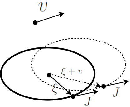
Figure 1: The unit ball of $\tilde{F}$ (punctured line) is the $v$-translation of that of $F$ (bold line). If a vector $J$ is tangent to the unit ball of $F$ at $\xi$, it is tangent to the unit ball of $\tilde{F}$ at $\xi+v$

Equivalently, this can be reformulated as

$$\tilde{F}(x,\xi)=F(x,\xi-\tilde{F}(x,\xi)v(x)).$$ (1)

Indeed, the equation (1) is positively homogeneous, and for any $\xi$ such that $\tilde{F}(x,\xi)=1$ we have $F(x,\xi-v(x))=1$.

The first result of this note is a description of how geodesics, Jacobi vector fields and flag curvatures of $F$ and of $\tilde{F}$ are related, if the vector field $v$ is a Killing vector field for $F$, that is, if the flow of $v$ preserves $F$.

Theorem 1.

Let $F$ be a Finsler metric on $M^{n}$ admitting a Killing vector field $v$ such that $F(x,-v(x))<1$ for all $x\in M^{n}$. We denote by $\Psi_{t}$ the flow of $v$ and by $\tilde{F}$ the $v$-Zermelo deformation of $F$.

Then, for any $F$-arc-length-parameterized geodesic $\gamma$ of $F$, the curve $t\mapsto\Psi_{t}(\gamma(t))$ which we denote by $\tilde{\gamma}(t)$ is a $\tilde{F}$-arc-length-parameterized geodesic of $\tilde{F}$.

Moreover, for any Jacobi vector field $J(t)$ along $\gamma$ such that it is orthogonal to $\dot{\gamma}(t)$ in the metric $g_{(\gamma(t),\dot{\gamma}(t))}:=\frac{1}{2}d_{\xi}^{2}F^{2}_{(\gamma(t),\dot{\gamma}(t))}$, the pushforward $\tilde{J}(t)=\Psi_{t*}(J(t))$ is a Jacobi vector field for $\tilde{\gamma}(t)$ and is orthogonal to $\dot{\tilde{\gamma}}(t)$ in $\tilde{g}_{(\tilde{\gamma}(t),\dot{\tilde{\gamma}}(t))}:=\frac{1}{2}d_{\xi}^{2}\tilde{F}^{2}_{(\tilde{\gamma}(t),\dot{\tilde{\gamma}}(t))}.$

Moreover, flag curvatures $K$ and $\tilde{K}$ of $F$ and $\tilde{F}$ are related by the following formula: for any $x\in M$ and any “flag” $(\xi,\eta)$ with flagpole $\xi\in T_{x}M$ and transverse edge $\eta\in T_{x}M$, we have $K(x,\xi,\eta)=\tilde{K}(x,\xi+v,\eta)$ provided that $\xi+v$ and $\eta$ are linearly independent.

We do not pretend that the whole result is new and rather suggest that its certain parts are known. The first statement of Theorem 1 appears in [6]. We recall the arguments of A. Katok in Remark 1. The third statement was announced in [3] and follows from the recent paper [5]. Special cases when the metric $F$ is Riemannian were studied in details in e.g. [1, 8]. Though we did not find the second statement of Theorem 1, the one about the Jacobi vector fields, in the literature, we think it is known in folklore.

Unfortunately in all these references, the proof is by direct calculations, which are sometimes quite tricky and sometimes require a lot of preliminary work. One of the goals of this note is to show the geometry lying below Theorem 1 and to demonstrate that certain parts of Theorem 1 at least are almost trivial.

Our second result shows that Zermelo deformation with respect to a Killing vector field preserves the property of a Finsler metric to be a locally symmetric space. We will call a Finsler metric locally symmetric, if for any geodesic $\gamma$ the covariant derivative of the Riemann curvature (=Jacobi operator) vanished:

$$D_{\dot{\gamma}}R_{\dot{\gamma}}=0.$$ (2)

Here $D_{\dot{\gamma}}$ stays for the covariant derivative along the geodesic: $D_{\dot{\gamma}}=\nabla^{\dot{\gamma}}_{\dot{\gamma}}$. Both most popular Finslerian connections, Berwald and Chern-Rund connections, can be used as the Finslerian connection in the last formula, see e.g. [9, §7.3], whose notation we partially follow.

Remark 1.

In Riemannian geometry there exist two equivalent definitions of locally symmetric spaces: according to the “metric” definition, a space is locally symmetric if for any point there exists a local isometry such that this point is a fixed point and the differential of the isometry at this point is minus the identity. By the other “curvature” definition, a space is locally symmetric if the covariant derivative of the curvature tensor is zero. The equivalence of these two definitions is a classical result of E. Cartan. We see that our definition above is the generalization to the Finsler metrics of the “curvature” definition; it was first suggested in [4].

In the Finsler setup, both “metric” and “curvature” definitions are used in the literature, but they are not equivalent anymore: the symmetric spaces with respect to the “metric” definition are symmetric spaces with respect to the “curvature” definition, but not vice versa.

In fact, the “metric” definition is much more restrictive; in particular locally symmetric metrics in the “metric” definition are automatically Berwaldian [7, Theorem 9.2] and are clearly reversible. On the other hand, all metrics of constant flag curvature, in particular all Hilbert metrics in a strictly convex domain, are locally symmetric in the “curvature” definition, and are symmetric with respect to the “metric” definition if and only if the domain is an ellipsoid.

In view of this, the name “locally symmetric” is slightly misleading, since locally symmetric manifolds may have no (local) isometries. We will still use this terminology because it was used in the literature before.

Theorem 2.

Suppose that $F$ is a locally symmetric Finsler metric and $v$ a Killing vector field satisfying $F(x,-v(x))<1$ for all $x$. Then, the $v$-Zermelo deformation of $F$ is also locally symmetric.

All Finsler metrics in our paper are assumed to be smooth and strictly convex but may be irreversible.

2 Proofs.

2.1 Proof of Theorem 1.

Let $\gamma(t)$ be an arc-length-parameterized $F$-geodesic, we need to prove that the curve $t\mapsto\Psi_{t}(\gamma(t))$ is an arc-length-parameterized $\tilde{F}$-geodesic. In order to do it, observe that for any $F$-arc-length-parameterized curve $x(t)$ the $t$-derivative of $\Psi_{t}(x(t))$ is given by $\Psi_{t*}(\dot{x}(t))+v(\Psi_{t}(x(t)))$. Since the flow $\Psi_{t}$ preserves $F$ and $v$, it preserves $\tilde{F}$ and therefore

$$\tilde{F}\left(\Psi_{t}(x(t)),\Psi_{t*}(\dot{x}(t))+v(\Psi_{t}(x(t)))\right)=\tilde{F}\left(x(t),\dot{x}(t)+v(x(t))\right)=F\left(x(t),\dot{x}(t)\right).$$

The last equality in the formula above is true because, for any $\xi$ such that $F(x,\xi)=1$, we have $\tilde{F}\left(x,\xi+v(x)\right)=F(x,\xi)$ by the definition of the Zermelo deformation. Thus, if the curve $x(t)$ is $F$-arc-length-parameterized, then the curve $\Psi_{t}(x(t))$ is $\tilde{F}$-arc-length-parameterized.

This also implies that the integrals $\int F(x(t),\dot{x}(t))dt$ and $\int\tilde{F}\left(\Psi_{t}(x(t)),\dot{\left(\Psi_{t}(x(t))\right)}\right)dt$ coincide for all $F$-arc-length-parameterized curves $x(t)$. Since geodesics are locally the shortest arc-length parameterized curves connecting two points, for each arc-length parameterized $F$-geodesic $\gamma$ the curve $t\mapsto\Psi_{t}(\gamma(t))$ is a $\tilde{F}$-arc-length-parameterized geodesic as we claimed.

Remark 2.

Alternative geometric proof of the statement that for each arc-length parameterized $F$-geodesic $\gamma$ the curve $t\mapsto\Psi_{t}(\gamma(t))$ is a $\tilde{F}$-arc-length-parameterized geodesic is essentially due to [6]: consider the Legendre-transformation $T:T^{*}M^{n}\to TM$ corresponding to the function $\frac{1}{2}F^{2}$ and denote by $F^{*}$ the pullback of $F$ to $T^{*}M^{n}$,  $F^{*}:=F\circ T$. Next, view the vector field $v$ as a function on $T^{*}M$ by the obvious rule $\eta\in T^{*}_{x}M^{n}\mapsto\eta(v(x))$. It is known that the Hamiltonian flow corresponding to the function $v$ is the natural lift of the flow of the vector field $v$ to $T^{*}M$. Since $v$ is assumed to be a Killing vector field, the Hamiltonian flows of $F^{*}$ and of $v$ commute. Next, consider the function $\tilde{F}^{*}:=F^{*}+v$. If $v$ satisfies $F(x,-v(x))<1$, then the restriction of $\tilde{F}^{*}$ to $T_{x}M^{n}$ is convex, consider the Legendre-transformation $\tilde{T}:TM^{n}\to T^{*}M$ corresponding to the function $\frac{1}{2}(\tilde{F}^{*})^{2}$ and the pullback of $\tilde{F}^{*}$ to $TM^{n}$, it is a Finsler metric which we denote by $\tilde{F}$. It is a standard fact in convex geometry that the Finsler metric $\tilde{F}$ is the $v$-Zermelo-deformation of $F$. Since the Hamiltonian flows of $F^{*}$ and of $v$, which we denote by $\psi_{t}$ and $d^{*}\Psi_{t}$ , commute, the Hamiltonian flow of $\tilde{F}^{*}$ is simply given by

$$\tilde{\psi}_{t}=d^{*}\Psi_{t}\circ\psi_{t}.$$ (3)

Then, for any point $(x,\xi)\in TM$ with $F(x,\xi)=1$, the projections of the orbits of $\tilde{\psi}_{t}$ and of $\psi_{t}$ starting at this point are arc-length parameterized geodesics $\gamma$ of $F$ and $\tilde{\gamma}$ of $\tilde{F}$. By (3) we have $\tilde{\gamma}(t)=\Psi_{t}\circ\gamma(t)$ as we claimed.

Let us now prove the second statement of Theorem 1. Consider a Jacobi vector field $J(t)$ which are orthogonal to $\gamma$. We need to show that the pushforward $\tilde{J}(t)=\Psi_{t*}(J(t))$ is a Jacobi vector field for the $\tilde{F}$-geodesic $\tilde{\gamma}(t):=\Psi_{t}(\gamma(t))$. By the definition of Jacobi vector field there exists a family $\gamma_{s}(t)$ of geodesics with $\gamma_{0}=\gamma$ such that $J(t)=\frac{d}{ds}_{|s=0}\gamma_{s}(t)$, since $J(t)$ is orthogonal to $\gamma$ we may assume that all geodesics $\gamma_{s}(t)$ are arc-length parameterized. As we explained above, $\Psi_{t}(\gamma_{s}(t))$ is a family of $\tilde{F}$-geodesics; taking the derivative by $s$ at $s=0$ proves what we want.

Let us now show that $\tilde{J}$ is orthogonal to $\dot{\tilde{\gamma}}$. First observe that the condition that $J(t)$ is orthogonal to $\dot{\gamma}(t)$ is equivalent to the condition that $J(F):=\sum_{r}J^{r}\frac{\partial F}{\partial\xi_{r}}$ vanishes at $\dot{\gamma}(t)$ for each $t$. Indeed, consider the one-form $U\in T_{\gamma(t)}M^{n}\mapsto g_{\gamma(t),\dot{\gamma}(t)}(\dot{\gamma}(t)_{,}U)$. Because of the (positive) homogeneity of the function $F$ we have that at a point $\dot{\gamma}(t)\in T_{\gamma(t)}M^{n}$

$$g_{(\gamma(t),\dot{\gamma}(t))}(\dot{\gamma}(t)_{,}U)=U^{r}\frac{\partial F}{\partial\xi_{r}}.$$ (4)

Next, take Equation (1) and calculate the differential of the restriction of $\tilde{F}$ to the tangent space: its components are given by

$$\frac{\partial\tilde{F}}{\partial\xi_{i}}=\frac{1}{1+v(F)}\frac{\partial F}{\partial\xi_{i}}.$$ (5)

In this formula, the derivatives of the function $F$ are taken at $\xi\in T_{x}S^{2}$, and the derivatives of the function $\tilde{F}$ are taken at $\xi-\tilde{F}(x,\xi)v$. By $v(F)$ we denoted the function $\sum_{r}\frac{\partial F}{\partial\xi_{r}}v^{r}$.

In view of (5), $J(\tilde{F}):=\sum_{r}J^{r}\frac{\partial\tilde{F}}{\partial\xi_{r}}$ vanishes at $\dot{\gamma}(t)+v(\gamma(t))$, so $J(t)$ is orthogonal to $\dot{\gamma}(t)+v(\gamma(t))$ (the orthogonality is understood in the sense of $\tilde{g}_{(\gamma(t),\dot{\gamma}(t)+v(\gamma(t)))}$). Then, $\tilde{J}(t)=\Psi_{t*}(J(t))$ is $\tilde{g}_{(\tilde{\gamma}(t),\dot{\tilde{\gamma}}(t))}$ orthogonal to $\dot{\tilde{\gamma}}(t).$

Remark 3.

Geometrically, the just proved statement that $\tilde{J}$ is orthogonal to $\dot{\tilde{\gamma}}$, after the identification of $T_{\gamma(t)}M^{n}$ and $T_{\Psi_{t}(\gamma(t))}M^{n}$ by the differential of the diffeomorphism $\Psi_{t}$, corresponds to the following simple observation: if $J$ is tangent to the unit $F$-sphere at the point $\xi=\dot{\gamma}$, then it is also tangent to the unit $\tilde{F}$-sphere at the point $\xi+v$, see Fig. 1.

Let us now prove the third statement of Theorem 1, we need to show that $K(x,\xi,\eta)=\tilde{K}(x,\xi+v,\eta)$. We consider a $F$-geodesic $\gamma(t)$ with $\gamma(0)=0$ and $\dot{\gamma}(0)=\xi$ and the corresponding $\tilde{F}$-geodesic $\tilde{\gamma}(t)=\Psi_{t}(\gamma(t));$ since $\Psi_{0}=\textrm{Id}$, we have $\dot{\tilde{\gamma}}(0)=\dot{\gamma}(0)+v=\xi+v$.

Observe that by combining [2, Eqn. 6.16 on page 117] and [2, Eqn. 6.3 on page 108] we obtain

$$\begin{array}[]{lcl}\frac{1}{2}\frac{d^{2}}{dt^{2}}g(J(t),J(t))&=&g(D_{\dot{\gamma}(t)}D_{\dot{\gamma}(t)}J(t),J(t))+g(D_{\dot{\gamma}(t)}J(t),D_{\dot{\gamma}(t)}J(t))\\ &=&-K(\gamma(t),\dot{\gamma}(t),J(t))\left(g(\dot{\gamma}(t),\dot{\gamma}(t))g(J(t),J(t))-g(\dot{\gamma}(t),J(t))^{2})+g(D_{\dot{\gamma}}J,D_{\dot{\gamma}}J\right).\end{array}$$ (6)

We will assume that $J(0):=\eta$ is $g$-orthogonal to $\dot{\gamma}(0)$. As explained above this implies that $\dot{\tilde{\gamma}}(0)$ is $\tilde{g}$-orthogonal to $\tilde{J}(0)$. Then, by (6), the minimum of $\frac{d^{2}}{dt^{2}}g(J(t),J(t))_{|t=0}$ taken over all Jacobi vector fields $J$ along $\gamma$ which are equal to $\eta$ at $t=0$, is equal to $-K(x,\xi,\eta)g(\xi,\xi)g(\eta,\eta)$. An analogous statement is clearly true also for $\tilde{\gamma}$, $\tilde{g}$ and $\tilde{J}$: namely, the minimum of $\frac{d^{2}}{dt^{2}}\tilde{g}(\tilde{J}(t),\tilde{J}(t))_{|t=0}$ taken over all Jacobi vector fields $\tilde{J}$ along $\tilde{\gamma}$ which are equal to $\eta$ at $t=0$, is equal to $-\tilde{K}(x,\xi+v,\eta)\tilde{g}(\xi+v,\xi+v)\tilde{g}(\eta,\eta)$. Here we used the relation $\tilde{J}(0)=\Psi_{t*}(J(t))_{|t=0}=J(0)$. Finally, in order to show that $K(x,\xi,\eta)=\tilde{K}(x,\xi+v,\eta),$ it is sufficient to show that the function $t\mapsto g(J(t),J(t))$ is proportional, with a constant coefficient, to the function $t\mapsto\tilde{g}(\tilde{J}(t),\tilde{J}(t)).$

In order to prove this, let us first compare $g_{(\gamma(t),\dot{\gamma}(t))}=\frac{1}{2}d_{\xi}^{2}F^{2}_{(\gamma(t),\dot{\gamma}(t))}$ and

$$\tilde{g}_{(\tilde{\gamma}(t),\dot{\tilde{\gamma}}(t))}=\frac{1}{2}d_{\xi}^{2}\tilde{F}^{2}_{(\Psi_{t}\circ\gamma(t),\Psi_{t*}(\dot{\gamma}(t))+v(\Psi_{t}(\gamma(t))))}.$$

It is convenient to work in coordinates $(x_{1},...,x_{n})$ such that the entries of $v$ are constants, in these coordinates for each $t$ the differential of the diffeomorphism $\Psi_{t}$ is given by the identity matrix, so in these coordinates $J(t)=\tilde{J}(t)$ and $\dot{\tilde{\gamma}}(t)=\dot{\gamma}(t)+v(\gamma(t)).$

Differentiating (5), we get the second derivatives of $\tilde{F}$. They are given by

$$\frac{\partial^{2}\tilde{F}}{\partial\xi_{i}\partial\xi_{j}}=\frac{1}{1+v(F)}\frac{\partial^{2}F}{\partial\xi_{i}\partial\xi_{j}}-\frac{1}{(1+v(F))^{2}}\sum_{r}\left(\frac{\partial^{2}F}{\partial\xi_{i}\partial\xi_{r}}v^{r}\frac{\partial F}{\partial\xi_{j}}+\frac{\partial^{2}F}{\partial\xi_{j}\partial\xi_{r}}v^{r}\frac{\partial F}{\partial\xi_{i}}\right).$$ (7)

Again, all derivatives of the function $F$ are taken at $\xi$, and of the function $\tilde{F}$ are taken at $\xi-\tilde{F}(x,\xi)v(x)$. Note that one term in the brackets in (7) appears because we differentiate $\frac{1}{1+v(F)}$, and the other appears because the derivatives of $\frac{\partial F}{\partial\xi_{j}}$ are taken at $\xi-\tilde{F}(x,\xi)v(x)$. When we differentiate it, we also need to take into account the additional term $-\tilde{F}(x,\xi)v(x)$.

Now, in view of the formula $\frac{1}{2}d^{2}(\tilde{F}^{2})=\tilde{F}d^{2}\tilde{F}+d\tilde{F}\otimes d\tilde{F}$ we obtain from (7) the formula for $\tilde{g}_{ij}$:

$$\tilde{g}_{ij}=\frac{\tilde{F}}{1+v(F)}g_{ij}-\frac{\tilde{F}}{(1+v(F))^{2}}\sum_{r}\left(\frac{\partial^{2}F}{\partial\xi_{i}\partial\xi_{r}}v^{r}\frac{\partial F}{\partial\xi_{j}}+\frac{\partial^{2}F}{\partial\xi_{j}\partial\xi_{r}}v^{r}\frac{\partial F}{\partial\xi_{i}}\right)+\frac{1}{(1+v(F))^{2}}\frac{\partial F}{\partial\xi_{i}}\frac{\partial F}{\partial\xi_{j}}.$$ (8)

Let us now compare the length of $J$ in $g(x,\xi)$ with that of in $\tilde{g}(x,\xi+v)$. We multiply (8) by $J^{i}J^{j}$ and sum with respect to $i$ and $j$. Since by assumptions $J(F)=\sum_{r}J^{r}\frac{\partial F}{\partial\xi_{r}}$ vanishes at $\xi$, all terms in the sum but the first vanish. We thus obtain that the length of $J$ in $\tilde{g}$ is proportional to that of in $g$ with the coefficient which is the square root of $\frac{\tilde{F}}{1+v(F)}$.

But along the geodesic both $\tilde{F}$ and $v(F)$ are constant. Indeed, $v(F)$ is the “Noether” integral corresponding to the Killing vector field. Theorem 1 is proved.

2.2 Proof of Theorem 2.

First, observe that a Finsler metric is locally symmetric if and only if for any geodesic $\gamma$ and any Jacobi vector field $J$ along $\gamma$ the vector field $D_{\dot{\gamma}}J$ is also a Jacobi vector field. Indeed, the equation for Jacobi vector fields is

$$D_{\dot{\gamma}}D_{\dot{\gamma}}J+R_{\dot{\gamma}}(J)=0.$$ (9)

$D_{\dot{\gamma}}$-differentiating this equation, we obtain

$$D_{\dot{\gamma}}(D_{\dot{\gamma}}D_{\dot{\gamma}}J+R_{\dot{\gamma}}(J))=D_{\dot{\gamma}}D_{\dot{\gamma}}(D_{\dot{\gamma}}J)+R_{\dot{\gamma}}(D_{\dot{\gamma}}J)+\left(D_{\dot{\gamma}}R_{\dot{\gamma}}\right)(J)=0.$$

If $D_{\dot{\gamma}}J$ is a Jacobi vector field, $D_{\dot{\gamma}}D_{\dot{\gamma}}(D_{\dot{\gamma}}J)+R_{\dot{\gamma}}(D_{\dot{\gamma}}J)$ vanishes so the equation above implies $\left(D_{\dot{\gamma}}R_{\dot{\gamma}}\right)(J)=0$, and since it is fulfilled for all Jacobi vector fields we have $D_{\dot{\gamma}}R_{\dot{\gamma}}=0$ as we claimed.

Thus, we assume that for any geodesic and for any Jacobi vector field for $F$ its $D_{\dot{\gamma}}$ derivative is also a Jacobi vector field, and our goal is to show the same for $\tilde{F}$. Clearly, it is sufficient to show this only for Jacobi vector fields which are $g$-orthogonal to $\dot{\gamma}$. Note that for such Jacobi vector fields $D_{\dot{\gamma}}J$ is also orthogonal to $\dot{\gamma}$, since both $g_{(\gamma,\dot{\gamma})}$ and $\dot{\gamma}$ are $D_{\dot{\gamma}}$-parallel.

Take a (arc-length-parameterized) $F$-geodesic $\gamma$ and a point $P=\gamma(0)$ on it. Consider the geodesic polar coordinated around this point, let us recall what they are and their properties which we use in the proof.

Consider the (local) diffeomorphism of $T_{P}M^{n}\setminus\{0\}$ to $M^{n}$ which sends $\xi\in T_{P}M^{n}\setminus\{0\}$ to $\exp(\xi):=\gamma_{\xi}(1)$, where $\gamma_{\xi}$ is the geodesic starting from $P$ with the velocity vector $\xi$. As the local coordinate systems on $T_{P}M^{n}\setminus\{0\}$ we take the following one: we choose a local coordinate system $x_{1},...,x_{n-1}$ on the unit $F$-sphere $\{\xi\in T_{P}M^{n}\mid F(P,\xi)=1\}$ and set the tuple $\left(F(P,\xi),x_{1}\left(\frac{1}{F}\xi\right),...,x_{n-1}\left(\frac{1}{F}\xi\right)\right)$ to be the coordinates of $\xi$. Combining it with the diffeomorphism $\exp$, we obtain a local coordinate system on $M^{n}$. By construction, in this coordinate system each arc-length parameterized geodesics starting at $P$, in particular the geodesic $\gamma$, is a curve of the form $(t,\textrm{const}_{1},...,\textrm{const}_{n-1})$.

Next, consider the following local Riemannian metric $\hat{g}$ in a punctured neighborhood of $P$: for a point $\sigma(t)$ of this neighborhood such that $\sigma$ is a geodesic passing through $P$ we set $\hat{g}:=g_{(\sigma(t),\dot{\sigma}(t))}$.

It is known that in the polar coordinates the metric $\hat{g}$ is block-diagonal with one $1\times 1$ block which is simply the identity and one $(n-1)\times(n-1)$-block which we denote by $G$:

$$\hat{g}=\left(\begin{array}[]{cc}1&\\ &G\end{array}\right).$$

It is known, see e.g. [9, Lemma 7.1.4], that the geodesics passing through $P$ are also geodesics of $\hat{g}$, and that for each such geodesic the operator $\hat{\nabla}_{\dot{\gamma}}$, where $\hat{\nabla}$ is the Levi-Civita connection of $\hat{g}$, coincides with $D_{\dot{\gamma}}$.

Next, consider analogous objects for the metric $\tilde{F}$. As the local coordinate system on the unit $\tilde{F}$-sphere we take the following: as the coordinate tuple of $\tilde{\xi}$ with $\tilde{F}(P,\tilde{\xi})=1$ we take the coordinate tuple $(x_{1}(\xi),...,x_{n-1}(\xi))$, where $\xi:=\tilde{\xi}-v(P)$. (Recall that the $v$-parallel-transport sends the unit $F$-sphere to the unit $\tilde{F}$-sphere.)

By Theorem 1, in these coordinate systems each Jacobi vector field $J=(J_{0}(t),...,J_{n-1}(t))$ along $\gamma$ which is orthogonal to $\gamma$ is also a Jacobi vector field along $\tilde{\gamma}$, which is the $\tilde{F}$-geodesic such that $\tilde{\gamma}(0)=P$ and $\dot{\tilde{\gamma}}(0)=\dot{\gamma}(0)+v(P)$, and is orthogonal to $\tilde{\gamma}$. By (8), the corresponding block $\tilde{G}$ is given by $\tilde{G}=\frac{1}{1+v(F)}G$. Since the function $v(F)$ is constant along geodesics, the coefficients $\Gamma_{ij}^{k}$ of the Levi-Civita connection $\hat{\nabla}$ of $\hat{g}$ such that $i=0$ or $j=0$ coincide with that of for the analog for $\tilde{F}$. A direct way to see the last claim is to use the formula $\Gamma_{ij}^{k}=\frac{1}{2}g^{ks}\left(\frac{\partial g_{is}}{\partial x_{j}}+\frac{\partial g_{js}}{\partial x_{i}}-\frac{\partial g_{ij}}{\partial x_{s}}\right)$, where of course all indices run from $0$ to $n-1$ and the summation convention is assumed.

Then, in our chosen coordinate system, the formula for the covariant derivative in $\hat{\nabla}$ along $\gamma$ for vector fields which are orthogonal to $\gamma$ simply coincides with that of the formula for the corresponding objects for $\tilde{F}$. Then, for any $\tilde{F}$-Jacobi vector field $\tilde{J}$ orthogonal to $\dot{\tilde{\gamma}}$ we have that $\tilde{D}_{\dot{\tilde{\gamma}}}\tilde{J}$- is again a Jacobi vector field. Theorem 2 is proved.

Acknowledgments. The authors thank Sergei Ivanov for useful comments. V.M. was partially supported by the University of Jena and by the DFG grant MA 2565/4.

Patrick Foulon: Centre International de Rencontres Mathématiques-CIRM, 163 avenue de Luminy, Case 916, F-13288 Marseille - Cedex 9, France.
Email: foulon@cirm-math.fr

Vladimir S. Matveev: Institut für Mathematik, Fakultät für Mathematik und Informatik,
Friedrich-Schiller-Universität Jena, 07737 Jena, Germany.
Email: vladimir.matveev@uni-jena.de

References

- [1] D. Bao, C. Robles, Z. Shen, Zermelo Navigation on Riemannian manifolds. J. Diff. Geom. 66(2004), 377–435.
- [2] S.-S. Chern, Z. Shen, Riemann-Finsler geometry. Nankai Tracts in Mathematics, 6(2005). World Scientific Publishing Co. Pte. Ltd., Hackensack, NJ. x+192 pp.
- [3] P. Foulon, Ziller-Katok deformations of Finsler metrics. 2004 International Symposium on Finsler Geometry, Tianjin, PRC, 2004. 22–24.
- [4] P. Foulon, Locally symmetric Finsler spaces in negative curvature. C. R. Acad. Sci. 324(1997), no. 10, 1127–1132.
- [5] L. Huang and X. Mo, On the Flag Curvature of a class of Finsler metrics produced by the Navigation problem. Pac. J. Math. 277(2015), 149–168.
- [6] A. B. Katok, Ergodic properties of degenerate integrable Hamiltonian systems. Izv. Akad. Nauk SSSR. 37(1973), 775–778, English translation in Math. USSR-Isv. 7(1973), 535–571.
- [7] V. S. Matveev and M. Troyanov, The Binet-Legendre metric in Finsler geometry. Geom. Topol. 16(2012), no. 4, 2135–2170.
- [8] Z. Shen, Finsler manifolds of constant positive curvature. In: Finsler Geometry, Contemporary Math. 196 (1996), 83֭–92.
- [9] Z. Shen, Differential Geometry of Spray and Finsler Spaces. Kluwer Academic Publishers, Dordrecht,