date03102017

Effects of Nanoparticles on the Dynamic Morphology of Electrified Jets

Abstract

We investigate the effects of nanoparticles on the onset of varicose and whipping instabilities in the dynamics of electrified jets. In particular, we show that the non-linear interplay between the mass of the nanoparticles and electrostatic instabilities, gives rise to qualitative changes of the dynamic morphology of the jet, which in turn, drastically affect the final deposition pattern in electrospinning experiments. It is also shown that even a tiny amount of excess mass, of the order of a few percent, may more than double the radius of the electrospun fiber, with substantial implications for the design of experiments involving electrified jets as well as spun organic fibers.

Dynamic instabilities of charged polymeric liquid jets play a crucial role in many natural phenomena and industrial processes, such as electrospinning, ink-jet printing, electrospray, and many others [1, 2, 3, 4, 5].

In this Letter, we investigate the effects of nanoparticles (NPs) inserted in a polymeric liquid bulk on the resulting charged jet dynamics (see Fig. 1). Interest in this process has been spurred by the possibility of tailoring the material composition and the physical properties of nanocomposite nanofibers [6]. Examples include reinforced yarns with carbon nanotubes [7], fluorescent quantum dots embedded in fibers to show suppressed energy transfer [8] or single-photon coupling to optical modes transmitted in sub-wavelength waveguides[9], nanodiamonds loaded at high concentrations to obtain coatings for UV protection and scratch resistance [10], application of metal NPs to surface-enhanced Raman scattering[11] and to nonvolatile flash memories[12].

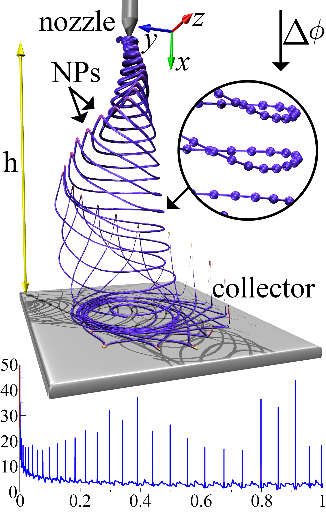
Figure 1: On the top, a simulation snapshot illustrating the electrospinning process: a jet is ejected at the nozzle and it is stretched towards a conductive collector by an external electric potential $\Delta\phi$ imposed between the nozzle and the collector. The color map used to drawn the jet is reported in Fig. 4. On the bottom, the decreasing profile of the jet radius $a$ (in $\mu$m) versus the curvilinear coordinate $\lambda\in[0,1]$, where $\lambda=0$ denotes the nozzle while $\lambda=1$ the last jet element closest to the collector without touching it.

In all aforementioned applications, the polymer component serves as a three-dimensional topological network of filaments in which NPs compose distributed functional domains. However, encoding the spatially-resolved information embedded in the nanofibers requires a detailed understanding of the way that electrospinning instabilities are modulated by the presence of NPs or clusters thereof, which can profoundly affect the ultimate jet morphology. Despite the major interest in above phenomena, to the best of our knowledge, numerical investigations of the dynamic behavior of electrified jets loaded with NPs are still lacking. In this Letter we take a first step along this line.

In the present study, we extend the discrete element model originally introduced by Reneker and co-workers [13], as discussed in Refs. [14, 15], and recently implemented in the open source code JETSPIN[16, 17].

Briefly, the jet is discretized into $n$ particle-like elements, representing a cylindrical jet segment, each labeled by the discrete index $i=1,..,n$, with mass $m_{i}$, charge $q_{i}$ and volume $V_{i}$. Each jet element is inserted at the nozzle at a mutual distance $l_{i}=l_{step}$ (initial length step of discretization), from the last bead, and imposing an initial jet volume $V_{i}=V_{0}$, corresponding to an initial jet radius $a_{0}=\sqrt{V_{0}/\pi l_{step}}$.

Under the effect of the electric potential $\Delta\phi$ (see Fig. 1), the jet elements move away from the nozzle undergoing a stretching process and a consequent decrease of the filament radius $a_{i}$ as a result of the volume conservation. For the sake of self-consistency, we review the basic model in Supplemental Material, while in the following we focus on the original features of the NP modeling. To this purpose, let us consider the $i$-th jet element with a spherical NP of radius $R$ embedded in the filament. The NP is assumed to be frozen in the polymeric bulk, hence following the same dynamic trajectory.

The mass (tagged by a star) of the cylindrical segment of volume $V_{i}$ including the NP is given by:

$$m_{i}^{*}=\left(V_{i}-\frac{4}{3}\pi R^{3}\right)\rho_{l}+\frac{4}{3}\pi R^{3}\rho_{NP},$$ (1)

where $\rho_{l}$ and $\rho_{NP}$ are the mass densities of the viscoelastic liquid and of the NP, respectively. Note that we are assuming $R<l_{i}$, so that each NP is confined to a single jet element. Further, we assume that only the polymeric bulk of the jet element is deformable. As a consequence, the viscoelastic stress imparts a force proportional to the cross sectional area $\pi{a_{i}^{*}}^{2}$ of the deformable part of the element, whose effective radius is defined as $a_{i}^{*}=\sqrt{\left(V_{i}-4/3\pi R^{3}\right)/\pi l_{i}}$.

$\rho_{l}$	$\rho_{NP}$	$\rho_{q}$	$a_{0}$	$h$
($\text{g}/\text{cm}^{3}$)	($\text{g}/\text{cm}^{3}$)	($\text{statC}/\text{cm}^{3}$)	(cm)	(cm)
0.84	10.49	$8.39\cdot 10^{-1}$	$5\cdot 10^{-3}$	16

$\alpha$	$\eta$	$Y$	$\Delta\phi$
(g/$\text{s}^{2}$)	(g/cm s)	(g/cm $\text{s}^{2}$)	(statV)
21.1	0.2	$5\cdot 10^{4}$	30.0

Table 1: Main simulation parameters in cgs units: $\rho_{l}$ density of liquid bulk, $\rho_{NP}$ density of NP, $\rho_{q}$ charge density, $a_{0}$ initial jet radius at the nozzle, $h$ distance between the nozzle and the collector, $\alpha$ surface tension, $\eta$ dynamic viscosity, $Y$ Young’s modulus, $\Delta\phi$ applied voltage. With the exception of $\rho_{NP}$ (mass density of Ag), all the parameters were taken from Ref. [16].

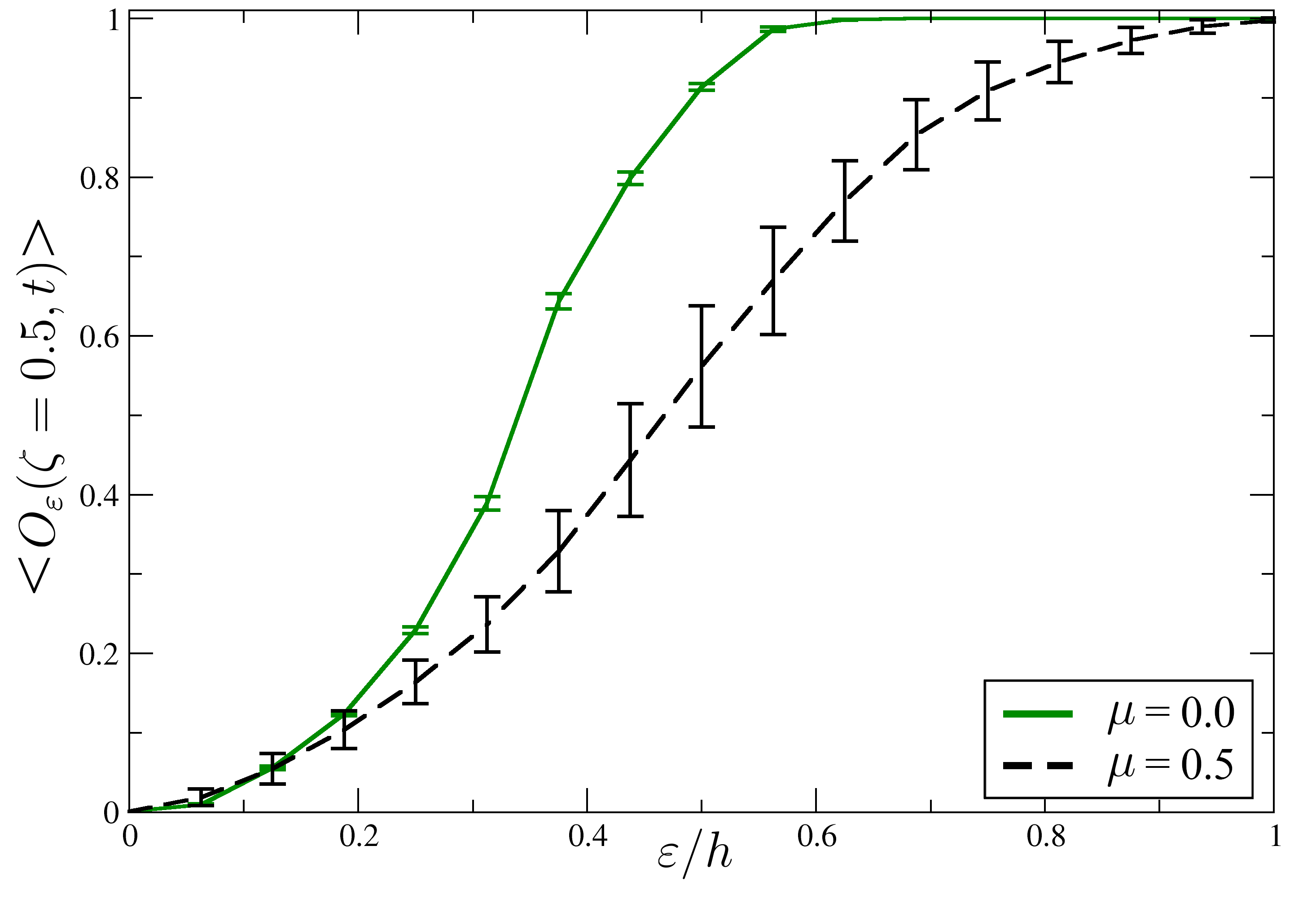
Figure 2: Mean value of SOP computed in the stationary regime ($\zeta=0.5$) as function of ratio $\varepsilon/h$. With $\varepsilon=8$, namely half distance between the nozzle and the collector, a neat separation between the cases $\mu=0$ and $\mu=0.5$, is well visible.

As a reference case, we take the simulation in absence of NPs (unloaded jet), with the simulation parameters assessed in Ref. [16] (see Table 1). The discretization step length is set to $0.02$ cm, in line with typical values reported in literature [13, 18, 19, 20, 21, 16], while the initial jet radius is set to $a_{0}=0.005$ cm.

We investigate seven different values of the particle radius, all other simulation parameters being kept fixed. We consider particles with mass density $\rho_{NP}=10.49\text{g}/\text{cm}^{3}$ (Ag), while the mass bulk density is set to $\rho_{l}$ is $0.84\text{g}/\text{cm}^{3}$. According to Eq 1, we choose the NP radius $R$ so as to prescribe specific values of the excess mass ratio $\mu=(m^{*}/m)-1$ at the injection point. In the above, $m^{*}$ and $m$ denote the inserted masses with and without NPs, respectively.

In all simulations, we load one jet element every five. Since each element represents a cylindric jet segment of length $0.02$ cm at the nozzle, we simulate a liquid jet with a series of NPs regularly spaced at a distance $0.1$ cm.

Figure 3: Dynamic evolution of $D_{0,\mu}$ versus time for three cases $\mu=0.05$, $\mu=0.2$ and $\mu=0.5$. The initial stage is characterized by a near-quadratic growth of the distance, with a mass-dependent acceleration. Upon hitting the collector, the distance undergoes oscillations around a non-zero mean. Both the amplitude and the non-zero mean are increasing functions of the excess-mass.

As a synthetic indicator of the departure between the jet path with and without NP, we introduce the global "distance" between two jet configurations:

$$D_{1,2}(t)=\int_{0}^{1}|\vec{r}_{2}(\lambda,t)-\vec{r}_{1}(\lambda,t)|\;d\lambda,$$ (2)

where $\lambda\in\left[0,1\right]$ is the curvilinear coordinate with $\lambda=0\,(1)$ denoting the nozzle (collector), respectively. This distance measures the cumulative point-by-point deviation between homologue (same $\lambda$) elements of the paths $1$ and $2$. The condition $D_{1,2}/h\ll 1$ denotes close-by configurations, as they occur in the unloaded limit $\mu\to 0$.

It is also convenient to define a local self-overlap parameter (SOP) as follows:

$$O_{\varepsilon}\left(\zeta,t\right)=\int_{0}^{1}H(\varepsilon-d(\lambda,\zeta))\;d\lambda$$ (3)

where $H$ is the Heaviside step function and $\zeta\in\left[0,1\right]$ specifies a generic point along the jet path, and $d(\lambda,\zeta)\equiv|\vec{r}(\lambda)-\vec{r}(\zeta)|$ is the local distance along the path. In the present context, low (high) SOP indicate high (low) stretch of the filament, which is qualitatively associated with local unstable (stable) behaviour. By definition, $O\to 0$ in the limit $\varepsilon\to 0$ and $O\to 1$ in the limit $\varepsilon\to\infty$, whatever the path morphology. As shown in Fig. 2, SOP works best away from both limits, namely for $\epsilon$ smaller than a typical macroscale, say the path length $L\sim h$, and larger than the smallest lengthscale, say, the helical pitch.

In Fig. 3 we report the observable $D_{0,\mu}$, versus time, computed for the unloaded case $\mu=0$ versus loaded ones, $\mu>0$. From this figure, we observe that the distance between the different configurations scales quadratically in time, indicating a free-fall-like regime before hitting the collector. As expected, the acceleration is a decreasing function of the mass excess parameter $\mu$. Upon hitting the collector, the distance shows periodic oscillations around a non-zero mean, of the order of a few centimeters, i.e. smaller but non-negligible as compared to nozzle-collector distance $h=16$ cm. As we shall detail shortly, these oscillations are interpreted as the signature of local inverted V-shape upturns of the trajectory, caused by the excess mass of the NPs, which tends to slow down the loaded segments relative to the unloaded ones.

Figure 4: On the top panel, two snapshots of the cases $\mu=0.05$ and $\mu=0.5$, taken at $t=0.01$ seconds alongside the color map, showing the colors used to draw the jet according to the corresponding mass density value $\rho$. On the bottom panel, the normalized 2D maps computed over the coordinates $y$ and $z$ of the collector for the two aforementioned cases collected over all the simulation runs with their respective color palettes defining the probability that a jet bead hits the collector at coordinates $y$ and $z$.

To gain further insight into the local morphology of the loaded jet, we inspect two snapshots taken at time $0.01$ seconds for the cases $\mu=0.05$ and $\mu=0.5$. As anticipated, this figure clearly shows that the slowing-down is due to the NPs, resulting from local inverted-V shaped upturns of the path configuration (higher mass density highlighted in yellow in Fig. 4).

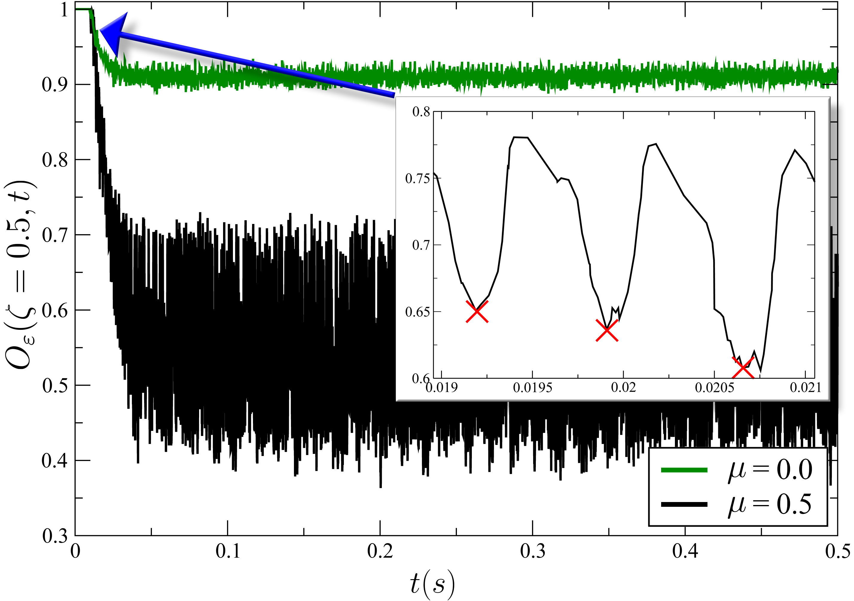
Figure 5: Dynamic evolution of $O_{\varepsilon}\left(\zeta=0.5,t\right)$ versus time for the two simulations with $\mu=0.0$ and $\mu=0.5$. In the inset we enlarge the dynamic for the case $\mu=0.5$ showing in red cross symbols whenever a NP is embedded in the jet point $\zeta=0.5$.

In Fig. 5, we report the time evolution of SOP for the cases $\mu=0$ and $\mu=0.5$. From this figure, we observe that both cases show a short decay to a steady state, with periodic oscillations on top of it. The case $\mu=0.5$ exhibits a much smaller SOP than $\mu=0$, and much larger oscillations all along, which is again a dynamic signature of the local upturns. Note that Fig. 5 refers to the mid-point $\zeta=0.5$, with a distance threshold $\varepsilon=8$ cm, i.e half the nozzle-collector separation, which is the best value to detect departures along the jet filament, as reported in Fig 2. It would be interesting to explore whether such collective observables could be monitored experimentally. This could be realized by means of recently proposed fast jet imaging using semi-transparent diffusing screens [22], properly combined with stereoscopic reconstruction techniques [23].

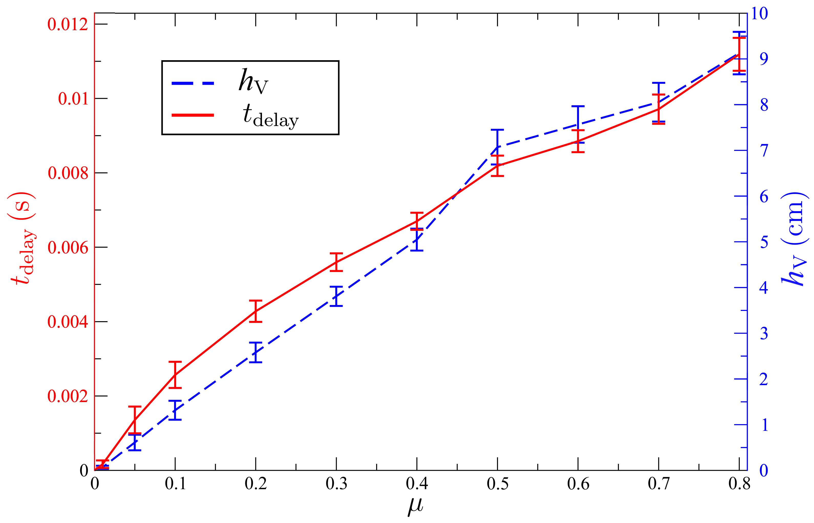
Figure 6: Averaged values of the V shape height $h_{\text{V}}$ (dashed blue line) and the delay time $t_{\text{delay}}$ (continuous red line) measured at the collector, as soon as the inverted V shape touches the conductive plate on both its sides. On the abscissas, we report the ratio $\mu$ of the masses related to the jet element with and without NP.

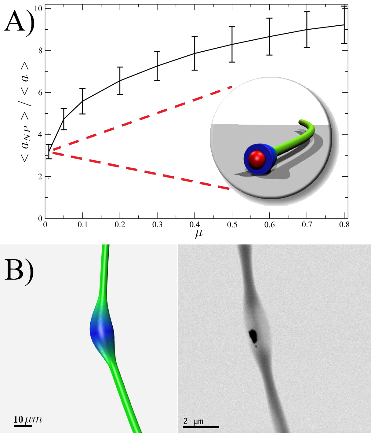
Figure 7: Panel A: Ratio $<a_{NP}>/<a>$ between average jet radii of fiber elements with and without NP for all the cases under investigation. On the abscissas, we report the ratio $\mu$ of the masses related to the jet element with and without NP as inserted at the nozzle. In the inset, the cross section of the fiber containing a NP (drawn in red) is shown for the simulation performed at $\mu=0.01$. Panel B: Left: a snapshot of a fiber segment containing a NP with $\mu=0.01$ (the same of the above inset although from a different perspective). Right: an experimental snapshot of an electrospun, particle-embedding polymer filament.

The changes in the jet morphology due to embedded NPs bears a significant impact also on the final deposition pattern of the nanofibers at the collector.

In Fig. 4, we show the in-plane probability of a jet bead hitting the collector around the coordinates $y$ and $z$ (the plate being perpendicular to $x$ direction) for the cases $\mu=0$ and $\mu=0.5$. From Fig. 4, we observe that the presence of the heaviest NPs shifts part of the deposited filament towards an outer shell, more than 8 cm away from the origin. The shift is also evident in Fig. 1, which reports a snapshot of the case $\mu=0.5$, with NPs (drawn in yellow) of the deposited fiber occupying the outermost area of the collector.

The effect is mainly due to the longer flight time of the jet segments containing NPs, which move at lower speed. The delay flight-time allows the filament to take and outward radial shift, while unloaded jet segments hit the collector along a well defined circle, with no radial shift due to the disturbance of NPs.

In Fig. 6, we report the delay flight-time as a function of $\mu$. A monotonically increasing trend is clearly visible, as a result of the V-shaped upturns due to the localized NPs. The same figure also reports the height of the V-shaped upturn, $h_{V}$, defined as the height of the triangle whose upper vertex is defined by the NP location, while the two lower vertices coincide with the touch-down locations on the collector. As expected, a similar trend as $t_{delay}$ is observed. In either cases, no abrupt change is observed, indicating no evidence of "critical" thresholds of the $\mu$ parameter.

In Fig. 7, we report the average fiber radius $<a>$, measured for both loaded ($a_{\text{NP}}$) and unloaded ($a$), jet elements for the cases under investigation, where brackets denote time average over the simulation time.

The figure shows a significant increase of the fiber radius as a function of $\mu$, which is sizeable already at $\mu=0.01$. In particular, we observe a rapid variation in the jet radius profile versus the curvilinear coordinate, resulting in a varicose-like shape of the filament. This delivers a fiber radius at the collector three times larger than the unloaded case, providing a concrete example of varicosity phenomena affecting the size of electrospun fibres. Varicosity effects are indeed detected in ongoing electrospinning experiments (panel B of Fig. 7). This figure shows a typical varicose profile, due to the insertion of a NP cluster with radius $R=0.4$ microns, leading to a local jet radius $a\sim 0.8$ microns, i.e. a factor two enhancement as compared to the unloaded case. The qualitative agreement between simulation (left) and experiment (right) is intriguing, and makes a subject of decided interest for future research.

References

- [1] A. L. Andrady, Science and technology of polymer nanofibers, Wiley, 2008.
- [2] A. L. Yarin, B. Pourdeyhimi, S. Ramakrishna, Fundamentals and Applications of Micro-and Nanofibers, Cambridge University Press, 2014.
- [3] D. Pisignano, Polymer Nanofibers: Building Blocks for Nanotechnology, no. 29, Royal Society of Chemistry, 2013.
- [4] M. M. Hohman, M. Shin, G. Rutledge, M. P. Brenner, Electrospinning and electrically forced jets. i. stability theory, Physics of fluids 13 (8) (2001) 2201–2220.
- [5] J. Eggers, E. Villermaux, Physics of liquid jets, Reports on progress in physics 71 (3) (2008) 036601.
- [6] C.-L. Zhang, S.-H. Yu, Nanoparticles meet electrospinning: recent advances and future prospects, Chemical Society Reviews 43 (13) (2014) 4423–4448.
- [7] F. Ko, Y. Gogotsi, A. Ali, N. Naguib, H. Ye, G. Yang, C. Li, P. Willis, Electrospinning of continuous carbon nanotube-filled nanofiber yarns, Advanced materials 15 (14) (2003) 1161–1165.
- [8] M. Li, J. Zhang, H. Zhang, Y. Liu, C. Wang, X. Xu, Y. Tang, B. Yang, Electrospinning: A facile method to disperse fluorescent quantum dots in nanofibers without förster resonance energy transfer, Advanced Functional Materials 17 (17) (2007) 3650–3656.
- [9] M. Gaio, M. Moffa, M. Castro-Lopez, D. Pisignano, A. Camposeo, R. Sapienza, Modal coupling of single photon emitters within nanofiber waveguides, ACS nano 10 (6) (2016) 6125–6130.
- [10] K. D. Behler, A. Stravato, V. Mochalin, G. Korneva, G. Yushin, Y. Gogotsi, Nanodiamond-polymer composite fibers and coatings, ACS nano 3 (2) (2009) 363–369.
- [11] C.-L. Zhang, K.-P. Lv, H.-P. Cong, S.-H. Yu, Controlled assemblies of gold nanorods in pva nanofiber matrix as flexible free-standing sers substrates by electrospinning, Small 8 (5) (2012) 648–653.
- [12] H.-C. Chang, C.-L. Liu, W.-C. Chen, Flexible nonvolatile transistor memory devices based on one-dimensional electrospun p3ht: Au hybrid nanofibers, Advanced Functional Materials 23 (39) (2013) 4960–4968.
- [13] D. H. Reneker, A. L. Yarin, H. Fong, S. Koombhongse, Bending instability of electrically charged liquid jets of polymer solutions in electrospinning, Journal of Applied physics 87 (9) (2000) 4531–4547.
- [14] M. Lauricella, G. Pontrelli, D. Pisignano, S. Succi, Dynamic mesh refinement for discrete models of jet electro-hydrodynamics, Journal of Computational Science 17 (2016) 325–333.
- [15] M. Lauricella, F. Cipolletta, G. Pontrelli, D. Pisignano, S. Succi, Effects of orthogonal rotating electric fields on electrospinning process, Physics of Fluids 29 (8) (2017) 082003.
- [16] M. Lauricella, G. Pontrelli, I. Coluzza, D. Pisignano, S. Succi, Jetspin: a specific-purpose open-source software for simulations of nanofiber electrospinning, Computer Physics Communications 197 (2015) 227–238.
- [17] The JETSPIN source code can be downloaded from the NANO-JETS project website at http://www.nanojets.eu/downloads.html.
- [18] T. Kowalewski, S. Blonski, S. Barral, Experiments and modelling of electrospinning process, Technical Sciences 53 (4) (2005) 385–394.
- [19] C. Thompson, G. G. Chase, A. Yarin, D. Reneker, Effects of parameters on nanofiber diameter determined from electrospinning model, Polymer 48 (23) (2007) 6913–6922.
- [20] Y. Sun, Y. Zeng, X. Wang, Three-dimensional model of whipping motion in the processing of microfibers, Industrial & Engineering Chemistry Research 50 (2) (2010) 1099–1109.
- [21] C. P. Carroll, Y. L. Joo, Discretized modeling of electrically driven viscoelastic jets in the initial stage of electrospinning, Journal of Applied Physics 109 (9) (2011) 094315.
- [22] M. Montinaro, V. Fasano, M. Moffa, A. Camposeo, L. Persano, M. Lauricella, S. Succi, D. Pisignano, Sub-ms dynamics of the instability onset of electrospinning, Soft matter 11 (17) (2015) 3424–3431.
- [23] G.-T. Michailidis, R. Pajarola, I. Andreadis, High performance stereo system for dense 3-d reconstruction, IEEE Transactions on Circuits and Systems for Video Technology 24 (6) (2014) 929–941.