We propose an analytical approach to the computation of tail probabilities of compound distributions whose individual components have heavy tails. Our approach is based on the contour integration method, and gives rise to a representation of the tail probability of a compound distribution in the form of a rapidly convergent one-dimensional integral involving a discontinuity of the imaginary part of its moment generating function across a branch cut. The latter integral can be evaluated in quadratures, or alternatively represented as an asymptotic expansion. Our approach thus offers a viable (especially at high percentile levels) alternative to more standard methods such as Monte Carlo or the Fast Fourier Transform, traditionally used for such problems. As a practical application, we use our method to compute the operational Value at Risk (VAR) of a financial institution, where individual losses are modeled as spliced distributions whose large loss components are given by power-law or lognormal distributions. Finally, we briefly discuss extensions of the present formalism for calculation of tail probabilities of compound distributions made of compound distributions with heavy tails.

1 Introduction

Many practical problems in applied science require accurate estimations of tails of compound distributions, i.e. random or non-random sums of random variables. In particular, in the context of financial risk management, to compute the operational Value at Risk (VAR) of a financial institution, the total loss resulting from aggregation of losses in different lines of business should be calculated at percentile levels of up to 99.9%. It is well known that ”classical” methods of calculation of aggregate distributions such as Monte Carlo, Fast Fourier Transform (FFT), or the Panjer recursion are all faced with various numerical issues at such high percentiles. Monte Carlo is robust but slow in suppressing the simulation noise. Likewise, the FFT and Panjer recursion methods become slow and lose accuracy, unless some special tricks are used, when computing such extreme tails of aggregate loss distributions.

We propose an analytical approach to calculation of tail probabilities of compound distributions where individual components have heavy tails. Our method employs a contour integration technique to compute tail probabilities expressed in terms of moment generating functions (MGFs) $M(z)$ of corresponding distributions. As is well known, in the case of extreme percentile levels such as 99.9%, such contour integral representations of tail probabilities give rise to exponentially small tail probabilities that are formally represented by highly oscillating contour integrals. We use analyticity in the complex $z$-plane in order to find a suitable deformation of the contour that produces a representation of the tail probability of in the form of a rapidly convergent real-valued one-dimensional integral. Our method is inspired by techniques developed for similar problems in physics where exponentially small probabilities expressed via highly oscillating contour integrals are encountered, in particular, in quantum mechanics [6] and quantum field theory [13]. To the best of our knowledge, such methods were not previously applied to the problem of computing tail probabilities of compound distributions with heavy tails.

As our procedure produces a representation of tail probabilities in terms of rapidly convergent integrals, the latter can be evaluated in quadratures, or alternatively represented as asymptotic expansions. Our method thus gives rise to a very efficient numerical scheme which avoids numerical issues that arise within the ”classical” methods such as Monte Carlo or FFT when computing such small tail probabilities.

While the method developed in this paper can be applied in many different problems that require accurate computation of tail probabilities for single or compound distributions with heavy tails, here we focus on one practical application. Specifically, we consider the problem of computing the Value at Risk (VAR) for aggregate operational losses of a financial institution. In this setting, the aggregate (compound) operational loss of each business unit of the institution can be modeled as a compound Poisson process, where each individual loss has a spliced distribution whose two component describe small and large losses, respectively. We consider in details two specifications of a single-unit large-loss component: a power-tail (Pareto) or lognormal, however the same method can be applied to other severity distributions as well, under certain technical conditions to be discussed below.

Furthermore, our analytical formulae assist a model selection process by directly capturing the dependence of the tail probability on the ”body” distribution (i.e. the distribution of small losses). As will be shown below, in models where single loss distributions have heavy tails, VAR at a high percentile level such as 99.9% is nearly independent of small losses, where small corrections to the independence law depend, for all practical purposes, only on the mean and variance of the distribution of small losses, but not on its higher moments. While the strict asymptotic (i.e. when VAR is yet much higher than 99.9%) decoupling of VAR from small losses for models with heavy tails was established a while ago in Ref.[1], our method gives an essentially exact solution that is valid for the actual level of 99.9% needed in practice, and recovers the result of Ref. [1] along with all corrections.

2 A spliced heavy-tailed distribution

In this paper, we are interested in tail probabilities of compound distributions whose individual components have heavy tails. To have a slightly more general framework, we model individual components as spliced distributions with the following probability density function (pdf):

$$f(x)\,=\,\left\{\begin{array}[]{clcr}(1-\omega)f_{1}(x)&\mbox{if $x\leq x_{0}$}\\ \omega f_{2}(x)&\mbox{if $x\geq x_{0}$}\\ \end{array}\right.$$ (3)

where both $f_{1}(x)$ and $f_{2}(x)$ are valid pdf’s (which means, in particular, that they separately integrate to one). While the second component $f_{2}(x)$ has a heavy tail, the first component $f_{1}(x)$ can be arbitrary. Obviously, the case of a pure heavy-tailed distribution is recovered when $\omega=0$ and $x_{0}=0$ (assuming that $x\geq 0$).

In the specific case of operational risk research that motivated the present work, a spliced loss distribution (3) can be used to model individual losses in a particular unit of measure (UoM), which further compound to produce the total loss in this UoM. We note that operational losses that belong in the same UoM may be very different from each other if they have qualitatively different origins. For example, for a large investment bank, legal losses can exceed other operational losses by a few orders of magnitude. A spliced loss severity distribution (3), where components $f_{1}(x)$ and $f_{2}(x)$ might have different scales, seems appropriate to model such cases, while reducing to a pure heavy-tailed distributions in other cases where the use of a spliced distribution is not required. For this reason, we stick in this paper to a more general definition of a heavy-tailed distribution as a spliced distribution (3). Bearing in mind this application of the presented formalism, in what follows we will occasionally refer to the random variable $x$ as the loss severity, though it might correspond to another random variable (e.g. the price of a security or a derivative instrument) in other settings.

The two components $f_{1}(x)$ and $f_{2}(x)$ in Eq.(3)) correspond to distributions of small ($x<x_{0}$) and large ($x\geq x_{0}$) losses, respectively, where $x_{0}$ is a right tail threshold. The mixing parameter $0\leq\omega\leq 1$ can be chosen e.g. by the continuity condition

$$(1-\omega)f_{1}(x_{0})=\omega f_{2}(x_{0})$$ (4)

Alternatively, we can integrate Eq.(3) from $0$ to $x_{0}$ and replace the unknown cumulative distribution $F(x)=\int_{0}^{x}f(s)ds$ by the empirical distribution. This provides a model-independent relation

$$\omega=1-F_{emp}(x_{0})$$ (5)

Note that if we fix $\omega$ using Eq.(5), then Eq.(4) can be considered as a constraint on the low-loss distribution $f_{1}(x)$ at the junction point $x_{0}$ (provided we know distribution $f_{2}(x)$), rather than a condition on $\omega$. In what follows, we do not dwell further on the modeling of $f_{1}(x)$ and keep it largely unspecified because, as will be shown below, VAR figures are mostly driven by the second, high-loss component $f_{2}(x)$. The dependence on $f_{1}(x)$ comes only through corrections in an asymptotic expansion in powers of $1/s$ (where $s$ is the VAR loss level), which are expected to be fairly small for sufficiently high percentile levels such as 99.9%.

In this paper, we consider two specifications of the severity distribution: a power-law and a lognormal law. Our choice is motivated by the observation that these two distributions seem to provide the best fit (of about equal quality) to large losses for the majority of UoMs of large financial institutions. In the next section, we concentrate on a power-law distribution, while the case of a lognormal distribution will be analyzed in Sect.4.

We consider the following power-law distribution for losses above the threshold $x_{0}$:

$$f_{2}(x)=f(x|x\geq x_{0})=\frac{\alpha-1}{x_{0}}\left(\frac{x}{x_{0}}\right)^{-\alpha}\equiv Cx^{-\alpha}$$ (6)

where $C=(\alpha-1)x_{0}^{\alpha-1}$ is the normalization constant. The tail distribution is

$$\bar{F}_{2}(x)=\int_{x}^{\infty}ds\,f_{2}(x)=\left(\frac{x}{x_{0}}\right)^{-(\alpha-1)}$$ (7)

The constant $\alpha>1$ in (6), (7) is called the exponent of the power law. Note that, given a choice of $x_{0}$, the exponent $\alpha$ is the only free parameter in the power-law distribution. The fitting procedures to compute parameters $\alpha$ and $x_{0}$ will be described below. For now, we note that the optimal value of $\alpha$ depends on $x_{0}$ logarithmically (i.e. mildly).

Power-law distributions (also known as Zipf or Pareto distributions) are ubiquitous in both nature and society, see e.g. [7] for a review, and are often characteristic of complex systems. Ref. [7] gives many examples of power-law distributions in language, demography, commerce, computer science, information theory, physics, astronomy, geology and so on. It seems that among ”wide” distributions (i.e. distributions for random variables that may vary by several orders of magnitude), a power-law distribution is more often a rule rather than an exception. For wide distributions that are not power-law, Ref. [7] mentions some (not too many) examples that are better described by a log-normal or a ”stretched exponential” (Weibull) distribution.

In our experiments with real-world operational loss datasets, we found that the power-law distribution (6) outperforms the Weibull and log-Weibull distributions in terms of both stability and quality of matching the data in the tail, while performing about equally well with a lognormal distribution.

3 Tail probabilities by contour integration

3.1 Moment generating functions

We start with the moment-generation function (MGF) of the power-law (Pareto) distribution:

$$M(z)=\mathbb{E}\left[e^{-zX}\right]=(\alpha-1)\left(zx_{0}\right)^{\alpha-1}\Gamma\left(1-\alpha,zx_{0}\right)\,,\;\;z\geq 0$$ (8)

Note that our sign convention is such that the MGF defined by (8) coincides with the Laplace transform of the distribution. In what follows, we will also use the characteristic function (CF) of $f(x)$ which is equal to the MGF evaluated at a purely imaginary argument:

$$\phi(z)=\mathbb{E}\left[e^{izX}\right]=M(-iz)$$ (9)

Note that the upper incomplete gamma function $\Gamma\left(s,z\right)$ has the following asymptotic behavior:

$$\Gamma(s,z)\,=\,\left\{\begin{array}[]{clcr}z^{s-1}e^{-z}\left[1+\frac{s-1}{z}+\ldots\right],&\mbox{if $|z|\rightarrow\infty,\,|\arg\,z|<\frac{3}{2}\pi$}\\ \Gamma(s)-z^{s}\left[\frac{1}{s}-\frac{z}{s+1}+\ldots\right],&\mbox{if $|z|\rightarrow 0,\,Re\,s<0$}\\ \end{array}\right.$$ (12)

This implies the following behavior of $M(z)$ in the limits $z\rightarrow 0$ and $|z|\rightarrow\infty$:

$$M(z)\,=\,\left\{\begin{array}[]{clcr}\frac{1}{x_{0}z}e^{-x_{0}z}\left[1-\frac{\alpha}{x_{0}z}+O(z^{-2})\right],&\mbox{if $|z|\rightarrow\infty,\,|\arg\,z|<\frac{3}{2}\pi$}\\ 1-\Gamma(2-\alpha)(x_{0}z)^{\alpha-1}+\frac{\alpha-1}{2-\alpha}x_{0}z+O(z^{2}),&\mbox{if $|z|\rightarrow 0,\,\alpha>1$}\\ \end{array}\right.$$ (15)

The upper incomplete gamma function $\Gamma\left(s,z\right)$ can be expressed in terms of the confluent hypergeometric function, also known as Kummer’s function:

$$\Gamma(s,z)=\Gamma(s)-\frac{z^{s}}{s}\Phi(s,1+s,-z)$$ (16)

Using this in (8), we obtain

$$M(z)=\Phi(1-\alpha,2-\alpha,-x_{0}z)-\Gamma(2-\alpha)\left(x_{0}z\right)^{\alpha-1}$$ (17)

Note that Kummer’s function $\Phi(a,b,z)$ is an analytic (holomorphic) function of $z$, while a power function in the second term in (17) has a branch cut singularity in the complex $z$-plane, which can be chosen to be the interval $[-\infty,0]$. We note that other heavy-tailed distributions, including in particular a lognormal distribution, have MGFs with similar analytic properties. Our approach developed below is very general and applies to any distribution whose MGF is analytic in a complex plane with a branch cut singularity. While the explicit form of the MGF is not used, the only additional requirement for the method to be applicable is that the MGF does not grow too fast in the left semi-plane. In particular, the MGF of the Pareto distribution is well behaved in this sense. Indeed, as shown in Eq.(15), $M(z)$ grows asymptotically $\sim e^{-x_{0}z}$ in the left semi-plane, but this divergence is integrable when calculating the tail probability (see below).

For the spliced distribution (3), the MGF function has a similar form to Eq.(17):

$$M(z)=R(z)-\omega\Gamma(2-\alpha)\left(x_{0}z\right)^{\alpha-1}$$ (18)

where we defined function $R(z)$ as follows:

$$R(z)=\omega\Phi(1-\alpha,2-\alpha,-x_{0}z)+(1-\omega)M_{1}(z)$$ (19)

where $M_{1}(z)$ stands for the MGF of the ”body” distribution $f_{1}(x)$. We assume that this distribution has all moments. In this case, $M_{1}(z)$ is an analytic function of $z$, and therefore function $R(z)$ is analytic as well. Note that $R(0)=1$.

To compute the MGF of a compound distribution, we need to specify a loss frequency model. For simplicity, we assume that the loss frequency for the time horizon $T=1$ is given by a Poisson distribution with intensity $\lambda$. The loss severity and loss frequency processes are assumed to be independent. Individual losses are independent as well. In this case, the MGF $M_{\lambda}(z)$ of the compound process (a random sum $X_{1}+\ldots+X_{n}$ of individual losses where $n$ is randomly drawn from the Poisson distribution) can be computed explicitly:

$$M_{\lambda}(z)=\sum_{n=0}^{\infty}\frac{(\lambda T)^{n}}{n!}e^{-\lambda T}\left[M(z)\right]^{n}=e^{\lambda T(M(z)-1)}$$ (20)

Note that as $e^{z}$ is an entire function (i.e. it is analytic in the whole complex plane), the compound MGF $M_{\lambda}(z)$ is analytic in the complex $z$-plane with the same branch cut singularity as the one present for the single loss MGF $M(z)$.

3.2 Tail probability as a contour integral

Recall the integral representation of the Heaviside step-function $\theta(x)$:

$$\theta(x)=\frac{e^{x\varepsilon}}{2\pi i}\int_{-\infty}^{\infty}\frac{e^{izx}}{z-i\varepsilon}dz$$ (21)

where $\varepsilon>0$ is arbitrary. In practice, it is convenient to employ the limit $\varepsilon\rightarrow+0$, which is what will be assumed in what follows. Using the residue theorem, it is easy to check that $\theta(x)$ defined by Eq.(21) is one when $x>0$, and zero when $x<0$. Indeed, when $x>0$, we close the contour in the upper semi-plane, and the integral is one due to the residue at the pole at $z=i\varepsilon$. Otherwise, if $x<0$, we close the contour in the lower semi-plane, and the integral equals zero.

Using Eq.(21), we can write the tail probability of a loss distribution with pdf $p(x)$ as follows:

$$\bar{F}(s)\equiv P\left(X>s\right)=\int_{0}^{\infty}dx\,p(x)\theta(x-s)=\int_{0}^{\infty}dx\,p(x)\frac{e^{(x-s)\varepsilon}}{2\pi i}\int_{-\infty}^{\infty}\frac{e^{iu(x-s)}}{u-i\varepsilon}du$$ (22)

Exchanging the order of two integrations, we obtain

$$\bar{F}(s)=\frac{e^{-s\varepsilon}}{2\pi i}\int_{-\infty}^{\infty}\frac{e^{-isu}}{u-i\varepsilon}\phi(u-i\varepsilon)du$$ (23)

where $\phi(z)$ stands for the characteristic function of distribution $p(x)$:

$$\phi(z)=\mathbb{E}\left[e^{izX}\right]=\int_{0}^{\infty}dx\,e^{izx}p(x)$$ (24)

Introducing a new variable $z$ by the relation $u=iz+i\varepsilon$, we obtain

$$\bar{F}(s)=-\frac{1}{2\pi i}\int_{-\varepsilon-i\infty}^{-\varepsilon+i\infty}\frac{e^{sz}}{z}\phi(iz)dz=-\frac{1}{2\pi i}\int_{-\varepsilon-i\infty}^{-\varepsilon+i\infty}\frac{e^{sz}}{z}M(z)dz$$ (25)

Note that contour of integration in Eq.(25) runs parallel to the imaginary axis. We assume that the MGF $M(z)$ is such that $e^{sz}M(z)\rightarrow 0$ for sufficiently large $s$ when $|z|\rightarrow\infty$ with $Re\,z<0$ (we will return to this point below when we consider specific applications). In this case, we can produce a closed contour by adding a semi-circle $C:|z|=R\rightarrow\infty,Re\,z<0$ in the left semi-plane to our initial open contour. By Jordan’s lemma, the value of the integral over the closed contour is equal to the value of the original integral with the open contour. Once we have a closed contour, we can use the Cauchy integral theorem and arbitrarily deform it within the analyticity domain without changing the value of the integral. As $M(z)$ is analytic in the complex $z$-plane with a branch cut on $z\in[-\infty,0]$, we can ”squeeze” the integration contour such that it runs first under the cut for $-\infty$ to $0$, then flips around the origin $z=0$, and runs back to $-\infty$ above the cut:

$$\bar{F}(s)=-\frac{1}{2\pi i}\int_{-\infty}^{0}dz\frac{e^{sz}}{z}M^{-}(z)-\frac{1}{2\pi i}\int_{0}^{-\infty}dz\frac{e^{sz}}{z}M^{+}(z)$$ (26)

where $M^{+}(z)$ and $M^{-}(z)$ stand for the values of the MGF $M(z)$ above and below the branch cut, respectively (see Fig. 1).

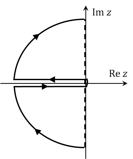
Figure 1: Integration contour for integral (25).

The two integrals in Eq.(26) do not cancel out due to a discontinuity of the imaginary part of $M(z)$ across the branch cut at $z=[-\infty,0]$. Setting $z=xe^{i\pi}$ and $z=xe^{-i\pi}$ with $x\geq 0$ at the upper and lower bank of the cut, respectively, the discontinuity is computed as follows:

$$\Delta\mathrm{Im}\,\,M(x)=\mathrm{Im}\,\,M(xe^{i\pi})-\mathrm{Im}\,\,M(xe^{-i\pi})$$ (27)

Using this in Eq.(26), we obtain

$$\bar{F}(s)=-\frac{1}{2\pi}\int_{0}^{\infty}dx\frac{e^{-sx}}{x}\Delta\mathrm{Im}\,\,M(x)$$ (28)

Eq.(28) constitutes our first main result. In the original complex-valued contour integral (25), the integrand becomes a strongly oscillating function when $s\rightarrow\infty$, which makes it difficult to accurately compute the tail probability in this limit. On the other hand, it is exactly this limit that is relevant for computing VAR at high percentile levels such as 99.9%. Using analyticity of the MGF in the complex plane with a cut, we have managed to reduce the complex integral (25) to a rapidly convergent integral (28) defined on the real axis. The latter integral can be computed very efficiently and accurately in quadratures. Clearly, numerical integration is much faster and more accurate than either Monte Carlo or a convolution method which are typically subject to a substantial numerical noise when computing tail probabilities at high percentiles. Using analyticity and contour integration, such numerical noise is filtered out in Eq.(28).

Note that the relation (28) is very general and applies to any distribution whose MGF $M(z)$ is analytic in a cut $z$-plane and well-behaved at infinity $|z|\rightarrow\infty,\,Re\,z<0$. It does not apply to distributions whose moment generating functions do not have a branch cut singularity, as in the letter case the discontinuity of the imaginary part of $M(z)$ would vanish. We will next consider uses of Eq.(28) to compute tail probabilities of both the single loss and compound loss distributions.

3.3 Tail probability of a single power-law distribution

As a check of our general relation (28), we apply it to compute the tail probability $P(X>s)$ of the single loss distribution given by Eq.(3) where the second component $f_{2}(x)$ is chosen to be a power-law distribution (6). Clearly, the answer in this case can be obtained by elementary means, and reads $P(X>s)=\omega\bar{F}_{2}(s)$ where $\bar{F}_{2}(x)$ is given by Eq.(7). Therefore, Eq.(28) should produce the same result.

Before proceeding with the calculation, we note that the MGF of a power-law distribution (or a distribution with a power-law tail as our Eq.(3)) is well behaved at infinity, as $e^{sz}M(z)\rightarrow 0$ when $s>x_{0}$ and $|z|\rightarrow\infty$ with $Re\,z<0$, as can be seen from Eq.(15). Therefore, Eq.(28) can be used in this case.

To compute the discontinuity of the MGF (18) across the branch cut, we note that it arises solely due to the second term in (18). Let $z=xe^{i\theta}$ along the cut, such that the path above the cut corresponds to $\theta=\pi$, and the path below the cut has $\theta=-\pi$. On these paths, the (main branch of the) power function $(x_{0}z)^{\alpha-1}$ takes values $-(x_{0}x)^{\alpha-1}e^{i\pi\alpha}$ and $-(x_{0}x)^{\alpha-1}e^{-i\pi\alpha}$, respectively. Therefore, the discontinuity of $\mathrm{Im}\,\,M(z)$ across the branch cut at $[-\infty,0]$ reads

$$\Delta\mathrm{Im}\,\,M(x) = \omega\Gamma(2-\alpha)(x_{0}x)^{\alpha-1}\mathrm{Im}\,\left(e^{i\pi\alpha}-e^{-i\pi\alpha}\right)=2\omega\Gamma(2-\alpha)\sin(\pi\alpha)(x_{0}x)^{\alpha-1}$$ (29)

$$= -\frac{2\omega\pi}{\Gamma(\alpha-1)}(x_{0}x)^{\alpha-1}$$

where at the last step we used the identity

$$\Gamma(x)\Gamma(1-x)=\frac{\pi}{\sin(\pi x)}$$ (30)

Introducing a new variable $y=x_{0}x$ and denoting $\hat{s}=s/x_{0}$, we obtain for the integral (28):

$$\bar{F}(s)=\frac{\omega}{\Gamma(\alpha-1)}\int_{0}^{\infty}dy\frac{e^{-\hat{s}y}}{y}y^{\alpha-1}=\omega\left(\frac{s}{x_{0}}\right)^{-(\alpha-1)}$$ (31)

We have thus verified that Eq.(28) correctly reproduces the tail probability for a single loss distribution with a power-law tail.

3.4 Tail probability of a compound power-law distribution

Now we turn to a more interesting application of relation (28). Namely, we use it to compute the tail probability of the compound distribution whose MGF is given by Eq.(20). No explicit closed form answer for this quantity is available, however we can compare our results with asymptotic expressions in the limit $s\rightarrow\infty$ that are available in the literature, as well as verify our results numerically.

Unlike the previous single-loss case, Eq.(28) cannot be straightforwardly used to compute the tail probability of the compound distribution, as the MGF (20) grows as an exponent of an exponent in the left semi-plane as implied by Eq.(15). However, this problem is easy to fix. To this end, let us identically represent the MGF (20) in the following form:

$$M_{\lambda}(z) = e^{\lambda T(M(z)-1)}=\sum_{n=0}^{n_{0}}\frac{(\lambda T)^{n}}{n!}e^{-\lambda T}\left[M(z)\right]^{n}+\sum_{n=n_{0}+1}^{\infty}\frac{(\lambda T)^{n}}{n!}e^{-\lambda T}\left[M(z)\right]^{n}$$ (32)

$$= \left(M_{\lambda}(z)-\mathcal{M}_{\lambda}(z)\right)+\mathcal{M}_{\lambda}(z)\equiv\tilde{M}_{\lambda}(z)+\mathcal{M}_{\lambda}(z)$$

where $n_{0}=\lfloor\frac{s}{x_{0}}\rfloor$ is the largest integer that is smaller or equal to the ratio $\frac{s}{x_{0}}$, and function $\mathcal{M}_{\lambda}(z)$ is a Taylor tail of $M_{\lambda}(z)$:

$$\mathcal{M}_{\lambda}(z)=\sum_{n=n_{0}+1}^{\infty}\frac{(\lambda T)^{n}}{n!}e^{-\lambda T}\left[M(z)\right]^{n}$$ (33)

while function $\tilde{M}_{\lambda}(z)$ is equal to $M_{\lambda}(z)$ with its Taylor tail subtracted. Now the first term $\tilde{M}_{\lambda}(z)$ in Eq.(32) is well-behaved in the left semi-plane when $s\geq x_{0}$, while the second term $\mathcal{M}_{\lambda}(z)$ is well-behaved in the right semi-plane where the product $e^{sz}\mathcal{M}_{\lambda}(z)\rightarrow 0$ as $z\rightarrow\infty$ when $s\geq x_{0}$.

Using Eq.(32), we can write the contour integral as follows:

$$\bar{F}(s)=-\frac{1}{2\pi i}\int_{-\varepsilon-i\infty}^{-\varepsilon+i\infty}\frac{e^{sz}}{z}\tilde{M}_{\lambda}(z)dz-\frac{1}{2\pi i}\int_{-\varepsilon-i\infty}^{-\varepsilon+i\infty}\frac{e^{sz}}{z}\mathcal{M}_{\lambda}(z)dz$$ (34)

We close the contour for the first integral in the left semi-plane and deform it following steps that led to Eq.(28), while for the second integral we close the contour in the right semi-plane and apply the residue theorem. We obtain

$$\bar{F}(s)=-\frac{1}{2\pi}\int_{0}^{\infty}dx\frac{e^{-sx}}{x}\Delta\mathrm{Im}\,\,\tilde{M}_{\lambda}(x)+\mathcal{M}_{\lambda}(0)$$ (35)

Here

$$\mathcal{M}_{\lambda}(0)=\sum_{n=n_{0}+1}^{\infty}\frac{(\lambda T)^{n}}{n!}e^{-\lambda T}=P(X>n_{0})$$ (36)

where $X\sim Po(\lambda)$ stands for a Poisson random variable driven by the Poisson law with intensity $\lambda T$. Thus $\mathcal{M}_{\lambda}(0)$ is the tail probability of the Poisson distribution. It can be estimated using the large deviation theory (see Appendix A for details):

$$\mathcal{M}_{\lambda}(0)=P\left(Po(\lambda T)>n_{0}\right)\sim e^{-n_{0}\left(\lambda T-\log\lambda T-1\right)}$$ (37)

Recalling that $n_{0}=\lfloor\frac{s}{x_{0}}\rfloor$, we see that the $\mathcal{M}_{\lambda}(0)$ term in Eq.(35) is exponentially suppressed for large $s$.

Next we turn to the first term in Eq.(35). We have

$$\tilde{M}_{\lambda}(z)=M_{\lambda}(z)-\mathcal{M}_{\lambda}(z)=e^{\lambda T(R(z)-1)}e^{-\omega\lambda T\Gamma(2-\alpha)\left(x_{0}z\right)^{\alpha-1}}-\mathcal{M}_{\lambda}(z)$$ (38)

We start with computing the discontinuity of the imaginary part of $M_{\lambda}(z)$. As function $R(z)$ is analytic, the first exponent in (38) is continuous across the branch cut, and discontinuity across the cut is due to the second exponent. Defining the values of the power function on different sides of the branch cut in the same way as was done in the previous section, we find the discontinuity of the imaginary part of $M_{\lambda}(z)$:

$$\Delta\mathrm{Im}\,\,M_{\lambda}(x) = e^{\lambda T(R(-x)-1)}\Delta\mathrm{Im}\,\,\left(e^{\omega\lambda T\Gamma(2-\alpha)(x_{0}x)^{\alpha-1}e^{i\pi\alpha}}\right)$$

$$= -2e^{\lambda T\Psi(x)}\sin\left[\frac{\pi\omega\lambda T}{\Gamma(\alpha-1)}\left(x_{0}x\right)^{\alpha-1}\right]$$

where for convenience we introduced function $\Psi(x)$ as follows:

$$\Psi(x)=R(-x)+\omega\Gamma(2-\alpha)\cos(\pi\alpha)\left(x_{0}x\right)^{\alpha-1}-1$$ (40)

Let us now consider the discontinuity of $\mathrm{Im}\,\,\mathcal{M}_{\lambda}(z)$ where function $\mathcal{M}_{\lambda}(z)$ is defined in Eq.(33). To this end, we note that for a fixed $z$, Eq.(33) can be viewed (up to a multiplier) as the tail probability of a Poisson distribution with intensity $\lambda M(z)$. Therefore, this function can be estimated using the large deviation result (37), provided we substitute $\lambda\rightarrow\lambda M(z)$:

$$\mathcal{M}_{\lambda}(z)=e^{\lambda T(M(z)-1)}P\left(Po(\lambda TM(z))>n_{0}\right)\sim e^{\lambda T(M(z)-1)}e^{-n_{0}\left(\lambda TM(z)-\log\lambda T-\log M(z)-1\right)}$$ (41)

We see that $\mathcal{M}_{\lambda}(z)$, and hence its imaginary part, is exponentially small in the limit $s\rightarrow\infty$. On the other hand, the term $\sim\Delta\mathrm{Im}\,\,M_{\lambda}(x)$ in Eq.(35) is only suppressed as a power of $1/s$, as will be clear below. Omitting exponentially suppressed contributions in Eq.(35) and introducing a new variable $y=x_{0}x$ as before, we finally obtain

$$\bar{F}_{\lambda}(s)=\frac{1}{\pi}\int_{0}^{\infty}\frac{dy}{y}e^{-\hat{s}y+\lambda T\Psi(y/x_{0})}\sin\left[\frac{\pi\omega\lambda T}{\Gamma(\alpha-1)}y^{\alpha-1}\right]$$ (42)

Eq.(42) constitutes our second main result. We have derived it as an application of our general relation (28). Up to exponentially suppressed terms, Eq.(42) provides an exact expression for the large-$s$ behavior of a random sum of i.i.d. random variables with power-law tails. As the integral (42) converges rapidly for $s\rightarrow\infty$, it can be evaluated very efficiently using quadratures. Alternatively, it can be expanded into an asymptotic series, as we discuss next.

3.5 Asymptotic expansion of the tail probability

As was mentioned above, as the integral (42) converges fast, a direct numerical integration is the most straightforward way to evaluate it. However, to better understand the asymptotic behavior of the tail probability of a compound Poisson loss process, it is useful to analyze an asymptotic expansion of the tail probability in the limit $s\rightarrow\infty$ that stems from Eq.(42). In particular, such asymptotic expansion allows one to analytically study the impact of a specification of the low-loss part of the loss distribution on the resulting VAR figures.

We start with an observation that for large $s\rightarrow\infty$, the integral (42) is dominated by small values of $y$. Therefore, we can evaluate (42) using Taylor expansions of functions $\Psi(\cdot)$ and $\sin(\cdot)$ that enter this expression. Using Eq.(19), we have

$$\Psi(y/x_{0})=\left(1-\omega\right)M_{1}(-y/x_{0})+\omega\Phi(1-\alpha,2-\alpha,y)+\omega\Gamma(2-\alpha)\cos(\pi\alpha)y^{\alpha-1}-1$$ (43)

Using the Taylor expansion of Kummer’s function

$$\Phi(a,b,z)=1+\frac{a}{b}z+\frac{1}{2!}\frac{a(a+1)}{b(b+1)}z^{2}+\ldots=\sum_{n=0}^{\infty}\frac{1}{n!}\frac{a^{(n)}}{b^{(n)}}z^{n}$$ (44)

(where $a^{(0)}=1$, $a^{(n)}=a(a+1)\ldots(a+n-1)$) and a general Taylor expansion of the low-loss MGF $M_{1}(-y/x_{0})$

$$M_{1}(-y/x_{0})=1+m_{1}y+m_{2}y^{2}+\ldots$$ (45)

we obtain the following small-$y$ expansions for functions entering Eq.(42):

$$\Psi(y/x_{0})=\omega\Gamma(2-\alpha)\cos(\pi\alpha)y^{\alpha-1}+c_{1}y+c_{2}y^{2}+\ldots$$

$$\sin\left[\frac{\pi\omega\lambda T}{\Gamma(\alpha-1)}y^{\alpha-1}\right]=\frac{\pi\omega\lambda T}{\Gamma(\alpha-1)}y^{\alpha-1}-\frac{1}{3!}\left(\frac{\pi\omega\lambda T}{\Gamma(\alpha-1)}y^{\alpha-1}\right)^{3}+\ldots$$ (46)

where

$$c_{1}=\frac{\omega}{1!}\frac{1-\alpha}{2-\alpha}+(1-\omega)m_{1}\,,\;\;c_{2}=\frac{\omega}{2!}\frac{1-\alpha}{3-\alpha}+(1-\omega)m_{2}$$ (47)

As $\Psi(y/x_{0})\rightarrow 0$ as $y\rightarrow 0$, we can additionally expand the exponent in Eq.(42) as $\exp\left(\lambda T\Psi(y/x_{0})\right)=1+\lambda T\Psi(y/x_{0})+\ldots$. Using this along with Eqs.(3.5), we obtain the following asymptotic expansion of the tail probability (42):

$$\bar{F}_{\lambda}(s) = \omega\lambda T\left(\frac{s}{x_{0}}\right)^{-(\alpha-1)}+a_{1}\left(\frac{s}{x_{0}}\right)^{-2(\alpha-1)}+a_{2}\left(\frac{s}{x_{0}}\right)^{-\alpha}$$ (48)

$$+ a_{3}\left(\frac{s}{x_{0}}\right)^{-3(\alpha-1)}+a_{4}\left(\frac{s}{x_{0}}\right)^{-(2\alpha-1)}+a_{5}\left(\frac{s}{x_{0}}\right)^{-(\alpha+1)}+\ldots$$

where

$$a_{1} = \left(\omega\lambda T\right)^{2}\frac{\Gamma(2-\alpha)\Gamma(2\alpha-2)}{\Gamma(\alpha-1)}\cos(\pi\alpha)=-\frac{1}{2}\left(\omega\lambda T\right)^{2}\frac{\left(\Gamma(2-\alpha)\right)^{2}}{\Gamma(3-2\alpha)}$$

$$a_{2} = \omega(\lambda T)^{2}c_{1}(\alpha-1)=\omega(\lambda T)^{2}(\alpha-1)\left(\omega\frac{1-\alpha}{2-\alpha}+(1-\omega)m_{1}\right)$$

$$a_{3} = -\frac{\pi^{2}}{3!}\Gamma(3\alpha-3)\left(\frac{\omega\lambda T}{\Gamma(\alpha-1)}\right)^{3}$$ (49)

$$a_{4} = \left(\omega\lambda T\right)^{2}\lambda Tc_{1}\frac{\Gamma(2-\alpha)\Gamma(2\alpha-1)}{\Gamma(\alpha-1)}\cos(\pi\alpha)=\frac{1}{2}\left(\omega\lambda T\right)^{2}\lambda T\frac{\left(\Gamma(2-\alpha)\right)^{2}}{\Gamma(2-2\alpha)}\left(\omega\frac{1-\alpha}{2-\alpha}+(1-\omega)m_{1}\right)$$

$$a_{5} = \omega(\lambda T)^{2}\left(c_{2}+\frac{\lambda T}{2}c_{1}^{2}\right)\frac{\Gamma(\alpha+1)}{\Gamma(\alpha-1)}=\omega(\lambda T)^{2}\alpha(\alpha-1)\left(c_{2}+\frac{\lambda T}{2}c_{1}^{2}\right)$$

Note that if we only keep the leading term in Eq.(48), we obtain

$$\bar{F}_{\lambda}(s)=\omega\lambda T\left(\frac{s}{x_{0}}\right)^{-(\alpha-1)}=\lambda T\bar{F}(s)\,,\;\;s\rightarrow\infty$$ (50)

which is a well-known result in the literature [1]. Eq.(50) is remarkable in that it shows that in the limit $s\rightarrow\infty$, the tail of the compound distribution with a power-law tail decouples from the low-loss region, as the parameter $\omega\lambda T$ entering this expression is the Poisson frequency of large losses and is therefore not sensitive to any additional small loss events that happen after the model is initially calibrated.

Now consider the structure of corrections $\sim a_{i}$ in Eq.(48). First, note that when $1<\alpha<2$, the term $\sim a_{1}$ is a leading correction, while for $\alpha>2$, the term $\sim a_{2}$ is a leading correction. If $1<\alpha<2$, i.e. the single loss distribution has an infinite mean, we see that the leading correction is still decoupled from the body of the distribution as it only depends on the combination $\omega\lambda T$. On the other hand, if $\alpha>2$ (so that the distribution has a finite mean), then the leading correction depends on the body of the distribution through its mean $m_{1}$. The sub-leading correction depends on $m_{1}$ if $1<\alpha<2$, or on both mean and variance $m_{1}$ and $m_{2}$, if $\alpha>2$. If we set $\omega=1$ (so that there is no low-loss ”body” of the distribution), our expression for $a_{1}$ coincides with an expression given in [10].

4 Tail probability of a random lognormal sum

In this section, we analyze random sums of lognormal random variables using a similar approach to that developed in the previous section. The added difficulty of analysis of a lognormal distribution is that its MGF is not available in an analytical form, but should rather be analyzed using its integral representation along with a saddle point approximation. As before, we start with the analysis of the tail probability of a single loss distribution.

4.1 MGF of a lognormal distribution in the left semi-plane

A random variable $Y=\exp(X)$ follows a lognormal distribution with mean $\mu$ and variance $\sigma^{2}$ if $X\sim N(\mu,\sigma^{2})$ is a normal random variable with the same mean and variance. The tail probability of a lognormal variable can be computed using elementary means:

$$\bar{F}(s)=P\left(Y>s\right)=P\left(X>\log s\right)=N\left(-\frac{\log s-\mu}{\sigma}\right)$$ (51)

where $N(x)$ stands for the cumulative normal distribution.

Now we represent the tail probability (51) as an inverse Laplace transform of its Laplace transform:

$$\bar{F}(s)=\frac{1}{2\pi i}\int_{-\varepsilon-i\infty}^{-\varepsilon+i\infty}dze^{sz}\bar{\mathcal{F}}(z)$$ (52)

where $\bar{\mathcal{F}}(z)$ stands for the Laplace transform of the tail probability

$$\bar{\mathcal{F}}(z)=\int_{0}^{\infty}dxe^{-zx}N\left(-\frac{\log x-\mu}{\sigma}\right)=-\frac{1}{z}\frac{1}{\sqrt{2\pi\sigma^{2}}}\int_{0}^{\infty}\frac{dx}{x}\exp\left(-zx-\frac{1}{2\sigma^{2}}\left(\log x-\mu\right)^{2}\right)$$ (53)

where we used integration by parts to get the second equation. Comparing Eq.(52) with Eq.(25) and using (53), we find the MGF

$$M(z)=\frac{1}{\sqrt{2\pi\sigma^{2}}}\int_{0}^{\infty}\frac{dx}{x}\exp\left(-zx-\frac{1}{2\sigma^{2}}\left(\log x-\mu\right)^{2}\right)$$ (54)

which of course can also be obtained directly from the definition of the MGF. Note that Eq.(54) defines the MGF $M(z)$ for $Re\,z\geq 0$. Its value in the left semi-plane $Re\,z<0$ is defined by analytical continuation as described below. Prior to doing this, we note that using the identity

$$\theta(x>s)=-\frac{1}{2\pi i}\int_{-\varepsilon-i\infty}^{-\varepsilon+i\infty}\frac{dz}{z}e^{z(s-x)}$$ (55)

we can verify that substituting Eq.(53) into Eq.(52), interchanging the orders of integrals over $z$ and $x$, and closing the contour in the right semi-plane, we reproduce (51).

Now instead of closing the integration contour in Eq.(52) in the right semi-plane, we want to use analytical properties of the MGF (54) to produce a different expression for the tail probability (52). To this end, we note that the MGF (54) is an analytic function of $z$ in a cut plane with a branch cut for $z\in[-\infty,0]$. The branch cut singularity in the $z$-plane arises due to a branch cut singularity of the integrand of (54) in the $x$-plane due to multivaluedness of the logarithm.

To find the MGF $M(z)$ in the left semi-plane $Re\,z<0$, one should analytically continue the integral (54). Let $z=\xi e^{i\theta}$ where $\xi=|z|\geq 0$. For $\frac{\pi}{2}<\theta<\frac{3\pi}{2}$, the real part of $z$ becomes negative, and to keep the integral convergent, we have to rotate the integration line in the $x$-plane by $-\theta$. This gives

$$M\left(\xi e^{i\theta}\right)=\frac{1}{\sqrt{2\pi\sigma^{2}}}\int_{C}\frac{dx}{x}\exp\left(-x\xi e^{i\theta}-\frac{1}{2\sigma^{2}}\left(\log x-\mu\right)^{2}\right)$$ (56)

where the integration contour is a ray $\{C:\,\arg(x)=-\theta,\,Re\,x\geq 0\}$. Changing the variable to $y=xe^{i\theta}$, we obtain

$$M\left(\xi e^{i\theta}\right)=\frac{1}{\sqrt{2\pi\sigma^{2}}}\int_{0}^{\infty}\frac{dy}{y}\exp\left(-y\xi-\frac{1}{2\sigma^{2}}\left(\log y-\mu-i\theta\right)^{2}\right)$$ (57)

Note that $M\left(\xi e^{\theta}\right)\rightarrow 0$ as $\xi\rightarrow\infty$, therefore if we close the contour in Eq.(52) in the left semi-plane, the integral over an infinite semi-circle vanishes by Jordan’s lemma. Deforming the integration contour in (52) in a similar way to steps taken above in the derivation of Eq.(28), the tail probability is now expressed in terms of a discontinuity of $\mathrm{Im}\,\,M(z)$ across the branch cut on $z\in[-\infty,0]$, as in Eq.(28):

$$\bar{F}(s)=-\frac{1}{2\pi}\int_{0}^{\infty}dx\frac{e^{-sx}}{x}\Delta\mathrm{Im}\,\,M(x)$$ (58)

The discontinuity across the cut can be found using Eq.(57):

$$\Delta\mathrm{Im}\,\,M(x) = \mathrm{Im}\,\,M\left(xe^{i\pi}\right)-\mathrm{Im}\,\,M\left(xe^{-i\pi}\right)$$ (59)

$$= 2\frac{\exp(\frac{\pi^{2}}{2\sigma^{2}})}{\sqrt{2\pi\sigma^{2}}}\int_{0}^{\infty}\frac{dy}{y}\exp\left(-xy-\frac{1}{2\sigma^{2}}\left(\log y-\mu\right)^{2}\right)\sin\left(\frac{\pi}{\sigma^{2}}\left(\log y-\mu\right)\right)$$

$$= 2\frac{\exp(\frac{\pi^{2}}{2\sigma^{2}})}{\sqrt{2\pi\sigma^{2}}}\int_{-\infty}^{\infty}dt\exp\left(-xe^{\mu+t}-\frac{1}{2\sigma^{2}}t^{2}\right)\sin\left(\frac{\pi}{\sigma^{2}}t\right)$$

Note that $\Delta\mathrm{Im}\,\,M(x)\rightarrow 0$ when $x\rightarrow 0$ (as the integrand in (59) becomes an odd function in this limit). Moreover, all terms of the Taylor expansion in the integrand result in converging integrals which all equal zero. This is a manifestation of non-analyticity of $M(z)$ at $z=0$.

To produce non-vanishing results for both $\mathrm{Im}\,M\left(xe^{i\pi}\right)$ and $\mathrm{Re}\,M\left(xe^{i\pi}\right)$, we return to Eq.(57) where we now set $\xi=x$, $\theta=\pi$ and change the variable to $z=\log\left(ye^{-\mu}\right)$:

$$M\left(xe^{i\pi}\right)=\int_{-\infty}^{\infty}\frac{dz}{\sqrt{2\pi\sigma^{2}}}\exp\left[\frac{1}{\sigma^{2}}\left(-\kappa e^{z}-\frac{1}{2}(z-i\pi)^{2}\right)\right]\equiv\int_{-\infty}^{\infty}\frac{dz}{\sqrt{2\pi\sigma^{2}}}\exp\left[\frac{1}{\sigma^{2}}g(z)\right]$$ (60)

where $\kappa=x\sigma^{2}e^{\mu}$ and function $g(z)$ is defined as follows:

$$g(z)=-\kappa e^{z}-\frac{1}{2}(z-i\pi)^{2}$$ (61)

Stationary points of functions $g(z)$ are zeros of the derivative

$$g^{\prime}(z)=-\kappa e^{z}-z+i\pi$$ (62)

Complex-valued stationary points can therefore be computed as

$$z_{0}=w+i\pi$$ (63)

where $w$ stands for real-valued solutions of the equation

$$w=\kappa e^{w}$$ (64)

In what follows, we restrict our analysis to the case when $\kappa$ is bounded from above as follows:

$$0\leq\kappa\leq\frac{1}{e}\;\;\Leftrightarrow\;\;0\leq x\leq\frac{1}{\sigma^{2}}e^{-\mu-1}$$ (65)

which seems sufficient for the analysis of asymptotic behavior at $s\rightarrow\infty$, as the integral (58) is dominated by small values of $x$ in this limit. Provided (65) is satisfied, Eq.(64) has two real roots $w_{1}$ and $w_{2}$ that are expressed in terms of Lambert functions $W_{0}(z)$ and $W_{-1}(z)$ (see [3]):

$$w_{1} = -W_{0}(-\kappa)\,,\;\;-1\leq-\kappa<\infty\,,\;\;W_{0}(-\kappa)\geq-1$$

$$w_{2} = -W_{-1}(-\kappa)\,,\;\;-\frac{1}{e}\leq-\kappa<0\,,\;\;W_{-1}(-\kappa)\leq-1$$ (66)

We note that the first saddle point $w_{1}$ also appears in a saddle point analysis of $M(z)$ in the right semi-plane $\mathrm{Re}\,z\geq 0$ (see Ref.[11]), while in our approach we concentrate on the behavior of $M(z)$ in the left semi-plane $\mathrm{Re}\,z\leq 0$, where the second saddle point $w_{2}$ appears in addition to $w_{1}$. As will be seen shortly, it is the second saddle point $w_{2}$ that determines the imaginary part of $M(z)$ along the branch cut at $z\in[-\infty,0]$.

The Lambert functions $W_{0}(x)$ and $W_{-1}(x)$ have the following expansions for small $x$ [3]:

$$W_{0}(x) = \sum_{n=1}^{\infty}\frac{(-n)^{n-1}}{n!}x^{n}=x-x^{2}+\frac{3}{2}x^{3}+\ldots$$

$$W_{-1}(x) = \log(-x)+\log\left(-\log(-x)\right)+\ldots$$ (67)

Note that when $\kappa\rightarrow 0$ (i.e. $x\rightarrow 0$), we have $w_{1}\ll 1$ and $w_{2}\gg 1$, so that the two saddle points are well separated from each other in this limit. Now compute the second derivative

$$g^{\prime\prime}(z_{0})=-\kappa e^{z_{0}}-1=\kappa e^{w}-1=w-1$$ (68)

We see that $g^{\prime\prime}\left(w_{1}\right)<0$, while $g^{\prime\prime}\left(w_{2}\right)\gg 1$. Therefore, a saddle-point contour should run parallel to the real axis when passing through $w_{1}$, and parallel to the imaginary axis when passing through $w_{2}$ (see below for more detail). Note that because the two saddle points are well-separated in the limit $\kappa\rightarrow 0$, calculations of the integral (60) amounts, in the saddle point approximation, to a sum of two separate saddle point integrals computed using quadratic approximations of $g(z)$ in the vicinity of points $w_{1}+i\pi$ and $w_{2}+i\pi$, respectively. Furthermore, as $g(w+i\pi)=w-\frac{1}{2}w^{2}$, we see that $g(w_{1}+i\pi)=O(1)$, while $g(w_{2}+i\pi)\rightarrow-\infty$ as $w_{2}\rightarrow\infty$ (i.e. $\kappa\rightarrow 0$). Therefore a contribution of the second saddle point $w_{2}$ to the real part $\mathrm{Re}\,M\left(xe^{i\pi}\right)$ is exponentially suppressed in comparison to a contribution of the first saddle point $w_{1}$, and thus can be safely neglected in the limit $\kappa\rightarrow 0$.

The saddle-point approximation is obtained using the standard arguments, see e.g. [9]. We expand $g(z)$ in a Taylor series around the saddle point $z_{0}$

$$g(z)=g(z_{0})+\frac{1}{2!}g^{\prime\prime}(z_{0})\left(z-z_{0}\right)^{2}++\frac{1}{3!}g^{\prime\prime\prime}(z_{0})\left(z-z_{0}\right)^{3}+\frac{1}{4!}g^{(4)}(z_{0})\left(z-z_{0}\right)^{4}+\ldots$$ (69)

(where the first order term is omitted as $g^{\prime}(z_{0})=0$), and introduce the following notation

$$g^{\prime\prime}(z_{0}) = \rho e^{i\theta}\;\;\;(\rho\geq 0)$$

$$z-z_{0} = te^{i\phi}$$ (70)

$$g(z) = u(x,y)+iv(x,y)$$

Note that $(\rho,\theta)=(1-w_{1},\pi)$ for $z_{0}=w_{1}+i\pi$, and $(\rho,\theta)=(w_{2}-1,0)$ for $z_{0}=w_{2}+i\pi$. All higher-order derivatives $g^{\prime\prime\prime},g^{(4)},\ldots$ are real-valued at both saddle points. Using this in Eq.(69), we obtain

$$u(x,y) = u(x_{0},y_{0})+\frac{1}{2}\rho t^{2}\cos\left(\theta+2\phi\right)+\sum_{n=4,6\ldots}\frac{1}{n!}g^{(n)}\left(z_{0}\right)t^{n}\cos\left(n\phi\right)$$

$$v(x,y) = v(x_{0},y_{0})+\frac{1}{2}\rho t^{2}\sin\left(\theta+2\phi\right)+\sum_{n=3,5\ldots}\frac{1}{n!}g^{(n)}\left(z_{0}\right)t^{n}\sin\left(n\phi\right)$$ (71)

A steepest descent path is therefore defined by the constraint $\cos\left(\theta+2\phi\right)=-1$. This produces $\phi=0$ for $w=w_{1}$, and $\phi=\pi/2$ for $w=w_{2}$. As $dz=e^{i\phi}dt$ near a saddle point, this means that $dz=t$ near $w_{1}$, and $dz=idt$ near $w_{2}$. Therefore, the steepest descent contour should run parallel to the real axis at $z=w_{1}+i\pi$, and parallel to the imaginary axis at $z=w_{2}+i\pi$, as was already mentioned above. A saddle point contour $C$ that passes through both saddle points and works for both the imaginary and real parts of the integral (60) can be obtained as a composition of three straight lines (see Fig. 2):

$$C\,=\,\left\{\begin{array}[]{clcr}x+i\pi,&\mbox{if $-\infty<\mathrm{Re}\,z<w_{2}$}\\ w_{2}+i\theta,&\mbox{if $\mathrm{Re}\,z=w_{2}\,,\;0\leq\theta\leq\pi$}\\ x,&\mbox{if $\mathrm{Re}\,z>w_{2}$}\end{array}\right.$$ (75)

Note that as $\cos\left(\theta+2\phi\right)=-1$ on the saddle point contour $C$, the second equation in (4.1) implies that $v(x,y)=v(x_{0},y_{0})$ along this contour. In our case, $v(x_{0},y_{0})=0$ for both saddle points, therefore $v(x,y)=\mathrm{Im}\,g(z)=0$ on $C$.

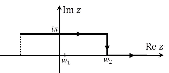
Figure 2: Integration contour for integral (60).

The last observation that $\mathrm{Im}\,g(z)=0$ along the steepest descent path $C$ implies that the contribution of the saddle point $w_{1}+i\pi$ (more precisely, the whole contribution of the first arc in (75)) drops off in the calculation of the imaginary part, because both the integrand and the integration contour become real for this integral after a change of variable $z=x+i\pi$:

$$\mathrm{Im}\,\int_{-\infty+i\pi}^{w_{2}+i\pi}\frac{dz}{\sqrt{2\pi\sigma^{2}}}\exp\left[-\frac{\kappa e^{z}+(z-i\pi)^{2}/2}{\sigma^{2}}\right]=\mathrm{Im}\,\int_{-\infty}^{w_{2}}\frac{dx}{\sqrt{2\pi\sigma^{2}}}\exp\left[-\frac{-\kappa e^{x}+\frac{1}{2}x^{2}}{\sigma^{2}}\right]=0$$

Therefore, even though the contribution of the second saddle point $w_{2}+i\pi$ is exponentially suppressed when computing the real part $\mathrm{Re}\,M\left(xe^{i\pi}\right)$ (see below), as the saddle point contour is complex-valued in the vicinity of $w_{0}^{(2)}+i\pi$, the second saddle point $w_{2}$ is the only one that determines the imaginary part of $M(z)$ along the branch cut. The dominant contribution to the imaginary part $\mathrm{Im}\,M\left(xe^{i\pi}\right)$ comes from integration over the second arc in the contour (75) (the integral over the third arc is exponentially suppressed in comparison to a contribution of the second arc, see below). Note that the contribution of $w_{1}$ to the imaginary part of $M(z)$ cancels out precisely due to a judicious choice of the integration contour (75). Unless such cancellation occurs, an accurate calculation of $\mathrm{Im}\,M\left(xe^{i\pi}\right)$ would be impossible for all practical purposes as it would require computing an exponentially suppressed quantity with a large ”numerical noise” that would be driven by an error in calculation of the contribution of the first arc in (75). The saddle point approximation to this integral produces the following result:

$$\mathrm{Im}\,M\left(xe^{i\pi}\right)=-\frac{1}{2}\frac{\exp\left(\frac{1}{\sigma^{2}}\left(w_{2}-\frac{1}{2}w_{2}^{2}\right)\right)}{\sqrt{w_{2}-1}}\left[1+\frac{\sigma^{2}}{8}\frac{w_{2}}{(w_{2}-1)^{2}}+O\left(w_{2}^{-2}\right)\right]$$ (76)

and $\mathrm{Im}\,M\left(xe^{-i\pi}\right)=-\mathrm{Im}\,M\left(xe^{i\pi}\right)$. The extra factor $\frac{1}{2}$ in Eq.(76) is due to the fact that the saddle point contour (75) involves only half of the line $[w_{2}-i\infty,w_{2}+i\infty]$ which would otherwise be obtained as a saddle point contour for a problem with a single saddle point at $w_{2}$ and $g^{\prime\prime}\left(w_{2}\right)>0$. Note that Eq.(76) is an asymptotic expansion valid for small $1/w_{2}\rightarrow 0$, i.e. for $\kappa\rightarrow 0$. Also note non-analyticity of this expression in $w$ (and hence in $\kappa$), which is due to the branch cut singularity of the square root function in (76).

To show that the contribution $I_{3}(\kappa)$ of the third arc of the saddle point contour (75) to the integral (60) is negligible as was promised above, we use the following inequalities:

$$|I_{3}(\kappa)|<\int_{w_{2}}^{\infty}\frac{dx}{\sqrt{2\pi}\sigma}\exp\left(-\kappa e^{x}-\frac{1}{2\sigma^{2}}(x^{2}-\pi^{2})\right)<\frac{\sigma}{2\sqrt{2\pi}w_{2}}\exp\left(-\frac{w_{2}}{\sigma^{2}}-\frac{1}{2\sigma^{2}}(w_{2}^{2}-\pi^{2})\right)$$

The second inequality here is obtained by noting that the maximum of the function $\phi(x)=-\kappa e^{x}-\frac{1}{2}\left(x^{2}-\pi^{2}\right)$ is attained at the left boundary $x=w_{2}$, and expanding $\phi(x)$ to linear order $\phi(x)=\phi(w_{2})+\phi^{\prime}(w_{2})\left(x-w_{2}\right)+\ldots$ to evaluate the integral. We see that $\mathrm{Im}\,I_{3}(\kappa)$ is exponentially suppressed in comparison with the contribution calculated in Eq. (76), and thus can be neglected in the limit $w_{2}\to\infty$ (i.e. $\kappa\to 0$). Likewise, $\mathrm{Re}\,I_{3}(\kappa)$ is exponentially suppressed relatively to a contribution due to the first arc of contour (75), as we will see next.

Turning to the calculation of the real part of $M(z)$ along the branch cut, it is now only the first saddle point $w_{1}$ (i.e. the first arc of the contour (75)) that determines the real part $\mathrm{Re}\,M\left(xe^{i\pi}\right)$, up to exponentially suppressed terms. The saddle point approximation produces the following result:

$$\mathrm{Re}\,M\left(xe^{i\pi}\right)=\frac{\exp\left(\frac{1}{\sigma^{2}}\left(w_{1}-\frac{1}{2}w_{1}^{2}\right)\right)}{\sqrt{1-w_{1}}}\left[1+\frac{\sigma^{2}}{8}\frac{w_{1}}{(1-w_{1})^{2}}+O\left(w_{1}^{2}\right)\right]$$ (77)

Expressions (76) and (77) will be used below to compute the tail distribution of a random sum of lognormal variables. Before doing that, we want to verify that Eq.(76) reproduces the right asymptotic behavior of a tail of a single lognormal loss when substituted in the general expression (58).

4.2 Tail probability of a single lognormal distribution

In this section, we check that our contour integral representation correctly reproduces the asymptotic behavior of the tail of the lognormal distribution (51):

$$\bar{F}(s)=N\left(-\frac{\log s-\mu}{\sigma}\right)=\frac{1}{\sqrt{2\pi}}\frac{\sigma}{\log s-\mu}\exp\left(-\frac{1}{2\sigma^{2}}\left(\log s-\mu\right)^{2}\right)+\ldots$$ (78)

As was shown above, it is only the second point $w_{2}$ that determines the imaginary part $\mathrm{Im}\,M(z)$ along the branch cut. Therefore, to lighten the notation, in this section we omit the index of the saddle point and write it simply as $w=w_{2}$ without any confusion. Note the integral (58) involves integration over $x$, while the asymptotic expression (76) is valid for an arbitrary fixed (and small) value $x\rightarrow 0$. The integral (58) could therefore be calculated, after a discretization on a grid $\{x_{i}\}$ ($i=1,2,\ldots$), by computing the saddle point $z_{0}(x_{i})$ for each value $x_{i}$ on the grid. However, it is much more convenient to change the integration variable $x\rightarrow w$ using Eq.(64) as a definition of the change of variables, thus avoiding a re-calculation of the saddle point for different values on the grid. The $x$ variable is found in terms of $w$ as follows:

$$x=\frac{1}{\sigma^{2}}e^{-\mu}w\exp(-w)$$ (79)

and the Jacobian $\mathcal{J}$ of the transformation is

$$\mathcal{J}=\left|\frac{\partial x}{\partial w}\right|=\frac{1}{\sigma^{2}}e^{-\mu-w}(w-1)$$ (80)

Using this in Eq.(58) along with Eq.(76) and truncating the integral at $x=\frac{1}{\sigma^{2}}e^{-\mu-1}$ (which is justified in the limit $s\rightarrow\infty$), we obtain

$$\bar{F}(s) = -\frac{1}{2\pi}\int_{0}^{\infty}dx\frac{e^{-sx}}{x}\Delta\mathrm{Im}\,\,M(x)\simeq-\frac{1}{2\pi}\int_{0}^{\frac{1}{\sigma^{2}}e^{-\mu-1}}dx\frac{e^{-sx}}{x}\Delta\mathrm{Im}\,\,M(x)$$ (81)

$$= \frac{1}{2\pi}\int_{1}^{\infty}\frac{dw}{w}\sqrt{w-1}\exp\left(\frac{1}{\sigma^{2}}\left(-swe^{-\mu-w}+w-\frac{1}{2}w^{2}\right)\right)\left[1+\frac{\sigma^{2}}{8}\frac{w}{(w-1)^{2}}+\ldots\right]$$

$$\equiv \frac{1}{2\pi}\int_{1}^{\infty}\frac{dw}{w}\sqrt{w-1}\exp\left(\frac{1}{\sigma^{2}}\Phi(w)\right)\left[1+\frac{\sigma^{2}}{8}\frac{w}{(w-1)^{2}}+\ldots\right]$$

where

$$\Phi(w)=-swe^{-\mu-w}+w-\frac{1}{2}w^{2}$$ (82)

This integral can be computed in the limit $s\rightarrow\infty$ using the saddle point approximation. Saddle points are found as solutions of the equation

$$\frac{d\Phi(w)}{dw}=\left(w-1\right)\left(se^{-w-\mu}-1\right)=0$$ (83)

This equation has two solutions $w_{1}=1$ and $w_{2}=\log s-\mu$, however, it is only the second solution $w_{2}$ that corresponds to the minimum of $\Phi(w)$, as can be easily checked by differentiation of Eq.(83). Therefore, we pick $w_{2}$ as the saddle point

$$w_{0}=\log s-\mu$$ (84)

Note that $w_{0}\gg 1$ when $s\rightarrow\infty$. We expand $\Phi(w)$ around this point:

$$\Phi(w)=\Phi(w_{0})+\frac{1}{2}\Phi^{\prime\prime}(w_{0})\left(w-w_{0}\right)^{2}+\ldots$$ (85)

We have

$$\Phi(w_{0}) = -\frac{1}{2}\left(\log s-\mu\right)^{2}$$

$$\Phi^{\prime\prime}(w_{0}) = -\log s+\mu+1$$ (86)

Omitting correction terms in (81), the leading order saddle point approximation reads

$$\bar{F}(s)=\frac{1}{\sqrt{2\pi}}\frac{\sigma}{\log s-\mu}\exp\left(-\frac{1}{2\sigma^{2}}\left(\log s-\mu\right)^{2}\right)+\ldots$$ (87)

which coincides with Eq.(78). We have therefore validated our result (76) using the known expression for the tail probability of a single-loss lognormal distribution.

4.3 Tail probability of a spliced distribution with a lognormal tail

Now we would like to discuss a practically important case of of a spliced loss severity distribution with a low-loss ”body” with a MGF $M_{1}(z)$ and a lognormal tail that starts at a junction point $x_{0}$. The MGF $M_{s}(z)$ of the spliced distribution is therefore

$$M_{s}(z)=\omega\tilde{M}(z)+(1-\omega)M_{1}(z)$$ (88)

where $\tilde{M}(z)$ stands for an MGF of a lognormal distribution truncated from below at $x_{0}$. As before, we assume that the MGF $M_{1}(z)$ of the ”body” is an analytic function of $z$, i.e. this distribution has all moments. The normalized truncated lognormal distribution has the following pdf:

$$\tilde{p}(x)=\theta(x\geq x_{0})\frac{\nu}{\sqrt{2\pi\sigma^{2}}}\frac{1}{x}\exp\left(-\frac{1}{2\sigma^{2}}\left(\log x-\mu\right)^{2}\right),\;\;\nu=\frac{1}{N\left(-\frac{\log x_{0}-\mu}{\sigma}\right)}$$ (89)

The MGF of a truncated lognormal distribution reads

$$\tilde{M}(z)=\nu\int_{x_{0}}^{\infty}\frac{dx}{\sqrt{2\pi\sigma^{2}}x}\exp\left(-xz-\frac{1}{2\sigma^{2}}\left(\log x-\mu\right)^{2}\right)$$ (90)

Note that apart from the constant multiplier $\nu$, the integral (90) only differs in the lower integration limit ($x_{0}$ instead of $0$) from the integral (54) that defines the MGF of an un-truncated lognormal distribution. Repeating steps leading to Eq.(60), but this time with the low bound of $x_{0}$, we obtain

$$\tilde{M}\left(xe^{i\pi}\right)=\nu\int_{\bar{w}_{0}}^{\infty}\frac{dz}{\sqrt{2\pi\sigma^{2}}}\exp\left[\frac{1}{\sigma^{2}}g(z)\right]\,,\;\;\bar{w}_{0}=\log x_{0}-\mu$$ (91)

where function $g(z)$ was defined in Eq.(61). The latter integral can now be evaluated using the saddle point approximation as was done above for an un-truncated lognormal distribution.

However, a detailed re-calculation is not necessary in this case. Recall that results of a saddle point approximation are not sensitive, to the leading order, to precise values of integration bounds as long as the latter are far away from a saddle point. This implies that as long as $\bar{w}_{0}\ll w_{2}$ (where $w_{2}$ is defined in Eq.(4.1)), the result for the imaginary part of $M_{s}\left(xe^{i\pi}\right)$ is the same (up to a constant multiplier) as for $M\left(xe^{i\pi}\right)$ (see Eq.(76)):

$$\mathrm{Im}\,M_{s}\left(xe^{i\pi}\right)=-\frac{\omega\nu}{2}\frac{\exp\left(\frac{1}{\sigma^{2}}\left(w_{2}-\frac{1}{2}w_{2}^{2}\right)\right)}{\sqrt{w_{2}-1}}\left[1+O\left(w_{2}^{-1}\right)\right],\;\;\left(\bar{w}_{0}\ll w_{2}\right)$$ (92)

To compute the real part of $M_{s}\left(xe^{i\pi}\right)$, we have to separately consider two cases: $\bar{w}_{0}<w_{1}$ and $\bar{w}_{0}>w_{1}$. In the first case, the first saddle point $w_{1}$ in Eqs.(4.1) lies inside of the integration interval, and the result for $\mathrm{Re}\,M_{s}\left(xe^{i\pi}\right)$ reads (see Eq.(77))

$$\mathrm{Re}\,M_{s}\left(xe^{i\pi}\right)=(1-\omega)\mathrm{Re}\,M_{1}\left(xe^{i\pi}\right)+\omega\nu\frac{\exp\left(\frac{1}{\sigma^{2}}\left(w_{1}-\frac{1}{2}w_{1}^{2}\right)\right)}{\sqrt{1-w_{1}}}\left[1+O\left(w_{1}\right)\right],\;\;\left(\bar{w}_{0}<w_{1}\right)$$ (93)

On the other hand, in the second case $\bar{w}_{0}>w_{1}$, the saddle point $w_{1}$ lies outside of the integration interval. In this case, the maximum of the integrand is attained at the left boundary of the integration interval. The asymptotic expression in this case reads

$$\mathrm{Re}\,M_{s}\left(xe^{i\pi}\right)=(1-\omega)\mathrm{Re}\,M_{1}\left(xe^{i\pi}\right)+\frac{\omega\nu\sigma}{\sqrt{2\pi}}\frac{\exp\left(\frac{1}{\sigma^{2}}\left(\bar{w}_{0}-\frac{1}{2}\bar{w}_{0}^{2}\right)\right)}{\bar{w}_{0}-\kappa e^{\bar{w}_{0}}}\left[1+O\left(w_{1}\right)\right],\;\;\left(\bar{w}_{0}>w_{1}\right)$$ (94)

Note that while in the previous expression (93) the second term depends on $x$ through a dependence of $w_{1}$ on $x$ (see Eqs.(4.1)), the second term in Eq.(94) is a constant in $x$, so that the $x$-dependence of $\mathrm{Re}\,M_{s}\left(xe^{i\pi}\right)$ in the case $\bar{w}_{0}>w_{1}$ arises solely due to the $x$-dependence of the MGF $M_{1}\left(xe^{i\pi}\right)$ of the ”body” of the distribution.

4.4 Tail probability of a compound distribution with a lognormal tail

In this section, we use our general relation (28) along with asymptotic relations (92)-(94) in order to compute the asymptotic expansion of the tail probability of a compound distribution where a single loss distribution is given by a spliced distribution with a low-loss ”body” with a MGF $M_{1}(z)$ and a lognormal tail that starts at a junction point $x_{0}$.

The MGF of a compound distribution with a Poisson frequency distribution is therefore

$$M_{\lambda}(z)=e^{\lambda T(M_{s}(z)-1)}$$ (95)

where $M_{s}(z)$ is defined in Eq.(88).

Recall that Eq.(28) can only be applied for MGFs that grow not faster than $e^{-x_{0}z}$ in the left semi-plane. This is the case in the present setting as $M(z)\rightarrow 0$ when $z=Re^{i\theta}$ with $R\rightarrow\infty$ and $\frac{\pi}{2}\leq\theta<\frac{3\pi}{2}$ (see Eq.(57)), which means that $M_{\lambda}(z)$ is bounded in the left semi-plane.

The discontinuity of the imaginary part of $M_{\lambda}(z)$ across the branch cut at $z\in[-\infty,0]$ reads

$$\Delta\,\mathrm{Im}\,M_{\lambda}\left(xe^{i\pi}\right)=2e^{\lambda T\left(\mathrm{Re}M_{s}\left(xe^{i\pi}\right)-1\right)}\sin\left[\lambda T\,\mathrm{Im}\,M_{s}\left(xe^{i\pi}\right)\right]$$ (96)

Using this in Eq.(28), we obtain

$$\bar{F}_{\lambda}(s)=-\frac{1}{\pi}\int_{0}^{\infty}\frac{dx}{x}e^{-sx+\lambda T\left(\mathrm{Re}M_{s}\left(xe^{i\pi}\right)-1\right)}\sin\left[\lambda T\,\mathrm{Im}\,M_{s}\left(xe^{i\pi}\right)\right]$$ (97)

Eq.(97) together with Eqs.(92)-(94) constitute our third main result that provides a rapidly convergent integral for a compound distribution of single loss distributions with lognormal tails. Similar to Eq.(42), this integral is dominated by small values of $x$ as $s\rightarrow\infty$, therefore we are justified in using asymptotic relations (92)-(94) to numerically evaluate the integral (97) in this limit. Also similar to Eq.(42), the low-loss component $f_{1}(x)$ effectively enters Eq.(97) only via its lowest moments, leading to a decoupling of the tail behavior of the compound distribution from individual small losses.

5 Compound distributions of compound heavy-tailed distributions

In this section, we briefly discuss possible extensions of the present formalism to compute tail probabilities of compound loss distributions where individual components are themselves compound distributions made of individual loss distributions with heavy tails. Such problem arise, in particular, when one computes total VAR of a financial institution having a number of different UoMs.

Let $X_{1},\ldots,X_{N}$ ($i=1,\ldots,N$) be total losses in $N$ different UoMs. Let $M_{\lambda}^{(i)}(z)$ be corresponding MGF’s for compound loss distributions for these UoMs, and $\lambda_{i}$ be their Poisson frequencies. The simplest assumption about the joint distribution of losses in all UoMs is to assume independence between them. Such assumption can be justified on the grounds of diffuculties of accurate estimation of correlation measures for operational losses, as well as the absence of any obvious mechanisms that would induce loss correlations between different UoMs. In this case, the MGF of the total loss $X=X_{1}+\ldots+X_{N}$ is given by the product of individual MGFs. Using Eq.(20), we obtain

$$M_{\lambda}(z)=\prod_{i=1}^{N}M_{\lambda}^{(i)}(z)=\prod_{i=1}^{N}\exp\left[\lambda_{i}T\left(M_{i}(z)-1\right)\right]=\exp\left[\sum_{i=1}^{N}\lambda_{i}T(M_{i}(z)-1)\right]$$ (98)

As this expression has the same functional form as Eq.(20), the tail probability of the compound compound distribution can be computed using the same relation (28) as was used above to compute tail probabilities of individual compound distributions.

Alternatively, if explicit modeling of dependencies between individual compound losses of different UoMs is deemed desired or necessary, there are multiple ways to introduces such dependences in a tractable way. One simple approach is to promote the Poisson intensities $\lambda_{i}$ into stochastic variables $\lambda_{i}({\bf Z})$ that depend on a low-dimensional set of $M$ common stochastic factors $\bf{Z}$. When one conditions on a realization of ${\bf Z}$, individual compound losses become independent, therefore the conditional tail probability $\bar{F}_{\lambda}\left(s|{\bf Z}\right)$ will still be given by Eq.(28) for each fixed value of ${\bf Z}$, and the unconditional tail probability would be obtained as follows:

$$\bar{F}_{\lambda}\left(s|{\bf Z}\right)=\int d{\bf Z}p({\bf Z})\bar{F}_{\lambda}\left(s|{\bf Z}\right)$$ (99)

where $p({\bf Z})$ is the probability density of ${\bf Z}$.

Finally, some standard copula models such as e.g. the Gaussian- or Student t-copula can be cast into an equivalent factor framework which ensures conditional independence of individual component losses. The conditional distribution of cumulative loss can be computed analytically using the saddle point method [4] in combination with methods presented above to compute marginal compound distributions. Details of such construction will be presented elsewhere.

6 Application to operational risk

In this section, we consider applications of our approach to calculation of the Operational Value at Risk (VAR) for a financial institution. We focus on the case where the large-loss component of an individual loss distribution is given by a power law distribution which is characterized by two parameters $\alpha$ and $x_{0}$. Once the threshold value of $x_{0}$ is specified, the value of $\alpha$ can be obtained using the expression obtained by the maximum likelihood method (see [2]):

$$\hat{\alpha}=1+N\left[\sum_{i=1}^{N}\log\frac{x_{i}}{x_{0}}\right]^{-1}$$ (100)

and the standard error of $\hat{\alpha}$ is

$$\sigma_{\alpha}=\frac{\hat{\alpha}-1}{\sqrt{N}}+O\left(\frac{1}{N}\right)$$ (101)

We illustrate our method with synthetic data produced using realistic model parameters that are similar to what is often observed in calibration to real world datasets.

We used the following values of parameters: $u=40,000$, $x_{0}=100,000$, $\alpha=2.2$, $\lambda=20$, $\omega=0.35$. The mean and variance of the body distribution are 63,877.92 and $2.625\cdot 10^{8}$, which corresponds to rescaled moments $m_{1}=-0.6388$ and $m_{2}=0.0131$.

The result obtained with our approach for the percentile level of 99.9% is shown in Fig. 3 where we also show results of MC simulation with 100 runs, each including 1,000,000 aggregate losses. We note that even for such a large number of MC trials the MC results are still quite noisy, which, in particular, makes computation of sensitivities difficult in the MC setting. Our analytical approach, by construction, is free of such defficiencies and allows accurate computation of both quantiles and their sensitivities.

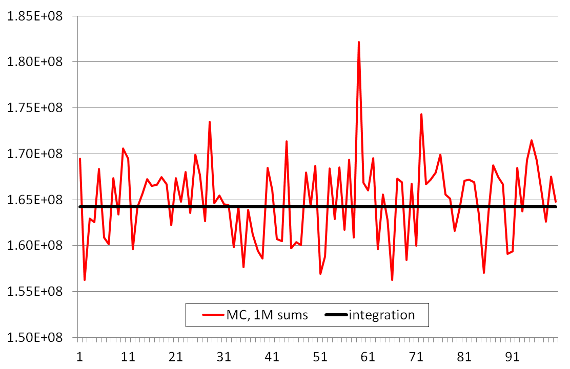
Figure 3: Integration vs MC simulation.

7 Summary

We have presented an analytical approach to computation of tail probabilities of compound heavy-tailed distributions, which is based on the contour integration method, and gives rise to a representation of the tail probability of a compound distribution in the form of a rapidly convergent real-valued one-dimensional integral. The latter integral can be evaluated in quadratures, or alternatively represented as an asymptotic expansion. While we only considered the case of a compound Poisson distribution where individual components have power-law or lognormal tails, our method can be extended to other settings with different specifications of individual component and/or frequency distribution, as long as its moment generating function has a branch cut singularity in the complex plane. We believe that the method proposed in this paper can offer a viable alternative to ”brute-force” numerical methods such as Monte Carlo, FFT or the Panjer recursion. Interestingly, this alternative appears especially attractive for high percentile levels, where these traditional approaches struggle, while the contour integration method starts to shine even more (in the sense that a convergent integral defining the tail distribution converges even faster as the percentile level increases).

Appendix A: Large deviations and Poisson tail probability

To apply the large deviation theory (see e.g. [12]) to estimation of the Poisson tail probability

$$P\left(Po(\lambda T)>n\right)=\sum_{k=n+1}^{\infty}\frac{(\lambda T)^{k}}{k!}e^{-\lambda T}$$ (A.1)

we use the equivalence of the Poisson event $Po(\lambda T)=n$ to the event of having $n$ arrivals by time $t=1$. If $Z_{i}$ with $i=1,2,\ldots$ stand for exponentially distributed random interarrival times, then $P\left(Po(\lambda T)>n\right)$ is the same as the probability of having the total arrival time for $n$ events to be less less than $t=1$

$$P\left(Po(\lambda T)>n\right)=P\left(Z_{1}+\ldots+Z_{n}<1\right)=P\left(\frac{Z_{1}+\ldots+Z_{n}}{n}<\frac{1}{n}\right)$$ (A.2)

To estimate this probability, we apply Cramer’s theorem [12]. We compute the rate function

$$I(z)=\sup_{x>0}\left(zx-\log\mathbb{E}e^{xZ_{1}}\right)=\sup_{x>0}\left(zx-\log\frac{\lambda T}{\lambda T-x}\right)=\lambda Tz-1-\log\lambda Tz$$ (A.3)

The Cramer theorem then states that

$$P\left(\frac{Z_{1}+\ldots+Z_{n}}{n}<\frac{1}{n}\right)\sim e^{-nI(1)}=e^{-n\left(\lambda T-\log\lambda T-1\right)}$$ (A.4)

References

- [1] K. Böcker and C. Klöppelberg, ”Operational VAR: a closed-form approximation”, RISK, December 2005, 90-93.
- [2] A. Clauset, C. R. Shalizi, and M.E.J. Newman, ”Power-law distributions in empirical data” (2007), available at http://arxiv.org/pdf/0706.1062.pdf.
- [3] R.M. Corless, G.H. Gonnet, D.E.G. Hare, D.J. Jeffrey, and D.E. Knuth, ”On the Lambert W function”, Advances in Computational Mathematics 5 (1996), 329 359.
- [4] I. Halperin, “CDO Pricing with Saddle Point Method”, JPM (2005).
- [5] L. Hernandez, J. Tejero, A. Su rez, and S. Carrillo-Men ndez (”Percentiles of Sums of Heavy-Tailed Random Variables: Beyond the Single-Loss Approximation”, Statistics and Computing, 24(3) (2014), pp. 377-397, available at http://arxiv.org/pdf/1203.2564.pdf.
- [6] L.D. Landau and E.M. Lifshitz, ”Quantum Mechanics”, Butterworth-Heinemann (1981).
- [7] M.E.J. Newman, ”Power Laws, Pareto Distributions and Zipf’s Law”, http://arxiv.org/pdf/cond-mat/0412004.pdf.
- [8] R. Lugannani and S. Rice, ”Saddlepoint approximations for the distribution of the sum of independent random variables”, Advances in Applied Probability, v.12 (1980), pp. 475- 490.
- [9] J. Mathews and R.L. Walker, Mathematical Methods of Physics, W.A. Benjamin, 1964.
- [10] A. Sahay, Z. Wan, and B. Keller, ”Operational risk capital: asymptotics in the case of heavy-tailed severity”, Journal of Operational Risk, v.2 (2007), 61-72.
- [11] C. Tellambura and D. Senaratne, ”Accurate Computation of the MGF of the Lognormal Distribution and its Application to Sum of Lognormals”, IEE Trans. on Communications, 58 (2010), 1568-1577.
- [12] S.R.S. Varadhan, Large Deviations and Applications, SIAM, Philadelphia (1984).
- [13] J. Zinn-Justin, ” The Principles of Instanton Calculus: a Few Applications”, in Recent Advances in Field Theory and Statistical Mechanics, Les Houches XXXIX (1982), ed. J.B. Zuber and R. Stora, Elsevier Science Publishers (1984).