Beyond the Unified Model

Abstract

The key elements of the Unified Model are reviewed. The microscopic derivation of the Bohr Hamiltonian by means of adiabatic time-dependent mean field theory is presented. By checking against experimental data the limitations of the Unified Model are delineated. The description of the strong coupling between the rotational and intrinsic degrees of freedom in framework of the rotating mean field is presented from a conceptual point of view. The classification of rotational bands as configurations of rotating quasiparticles is introduced. The occurrence of uniform rotation about an axis that differs from the principle axes of the nuclear density distribution is discussed. The physics behind this tilted-axis rotation, unknown in molecular physics, is explained on a basic level. The new symmetries of the rotating mean field that arise from the various orientations of the angular momentum vector with respect to the triaxial nuclear density distribution and their manifestation by the level sequence of rotational bands are discussed. Resulting phenomena, as transverse wobbling, rotational chirality, magnetic rotation and band termination are discussed. Using the concept of spontaneous symmetry breaking the microscopic underpinning of the rotational degrees is refined.

1 Introduction

This Focused Issue commemorates the 40-year Anniversary of the Nobel Prize for A. Bohr, B. R. Mottelson and L. Rainwater, which was awarded ”for the discovery of the connection between collective motion and particle motion in atomic nucleus and the development of the theory of the structure of the atomic nucleus based on this connection.” Before 1952, two apparently incompatible models coexisted. The Liquid Drop Model [1] describes the nucleus as a droplet of incompressible nuclear liquid, where the shape parameters are the degrees of freedom. As major achievements, it determined the stability of nuclei against spontaneous fission and explained the phenomenon of induced fission. The shell model considers the nucleus as a system of independent protons and neutrons confined to the spherical nuclear potential [2, 3]. It succeeded in explaining existence of special (”magic”) numbers of protons and neutrons for which nuclei are particularly strongly bound and it well accounted for excitation energies of these nuclei.

The experimental evidence for a substantial deformation of the nuclear charge deformation and for the existence of low-energy rotational excitations inspired A. Bohr and B. R. Mottelson to combine the two models to the Unified Model. In their pioneering papers [4, 5], they introduced the innovative concept of the coexistence and the interplay of collective and single particle degrees of freedom, which has become a fundamental of understanding low-energy nuclear structure. They realized that the collective motion of the density is accompanied by a corresponding motion of shell-model potential, which modifies the motion of the nucleons in the potential. The response of the nucleon ensemble determines the inertial parameters and the potential of the collective Hamiltonian. In addition, they assumed that the collective motion is slow compared to the single particle motion.

The Unified Model was extremely successful in accounting for the observation of collective and particle-like phenomena in one and the same nucleus. The concept has developed considerably during the succeeding years. In their contributions to this Focus Issue, D. R. Bes [8] and K. Heyde and J. L.Wood [7] review the history that lead to birth of the Unified Model and its subsequent development in a comprehensive way. A. Bohr and B. R. Mottelson expose in great detail the mature version of the Unified Model in their famous monograph Nuclear Structure Vol. II: Nuclear Deformations [6]. For a first encounter with the Unified Model, the excellent textbook Nuclear Collective Motion: Models and Theory by D. J. Rowe is recommended. A extended exposure of models describing the collective and single particle modes is given in Fundamentals of Nuclear Models by D. J. Rowe and J. L. Wood [10].

In the following I will refer to the ”Unified Model” as presented in these books. A central element of the theory is the presumption that the collective motion is slow as compared to the single particle motion, which simplifies the treatment of the coupling between collective and single particle degrees of freedom. The nucleonic orbitals adjust ”adiabatically” to the changing potential, which means, they are determined by the potential at given instant of time. Additional coupling terms due to the finite velocity of the changing potential are either neglected or taken into account in lowest order perturbation theory. The ”adiabatic approximation” shapes the interpretation of data in a fundamental way. For this reason it seems appropriate using the name ”Unified Model” when the adiabatic approximation is applicable. Clearly the concept of nucleons moving in a time-dependent potential extends beyond the realm of the Unified Model specified in this way. However, when the coupling between collective and single particle degrees of freedom becomes strong new phenomena emerge and it may be useful changing the perspective of looking on the data. Some of these new aspects beyond the Unified Model will be presented in my contribution.

The advances of experimental techniques after 1970, in particular the combination heavy ion accelerators with arrays of $\gamma$-detectors, provided new results that demonstrated the limitations of the Unified Model and stimulated the development of new theoretical approaches. My contribution will report on the progress in understanding the behavior of rapidly rotating nuclei, where the focus is on novel concepts and not on a full scale presentation of the theoretical approaches. Section 2 summarizes the essentials of the Unified Model and its microscopic foundation. The range of applicability is delineated by comparing its predictions with data. The non-adiabtic regime has been furthest explored in in the framework of the semiclassical rotating mean field approach. Section 3 lays out its simplest version based on the schematic pairing + quadrupole - quadrupole interaction, analyzes the symmetries and their observable consequences and introduces the Cranked Shell Model classification of the multi-band spectra. The central role of rotational frequency for the interpretation of the data and the appearance of uniform rotation about a tilted axis are discussed. Based on the concept of spontaneous symmetry breaking, the emergence and disappearance of collective degrees of freedom is analyzed in section 4. The definition collective angles is refined by changing the focus from the orientation of the deformed nuclear potential to the orientation in space of the nodal structure of the mean field many-body state. The new perspective accounts for band termination and magnetic rotation, which are phenomena beyond the Unified Model. The yrast states of spherical and weakly deformed nuclei are described as ”tidal waves” running over the nuclear surface. Section 5 lists some challenging phenomena beyond the Unified Model, for which the appropriate theoretical approaches are yet to be developed. Appendix A provides a semiclassical analysis of the interaction between the high-j particle orbitals and the deformed nuclear potential. Appendix B contains a table for navigating the paper.

The paper is meant as an introduction to structure of rotating nuclei on the graduate student level. I apologize to colleagues working in the field for repeating too many well known things and to newly interested ones for not having well enough explained certain things. To be self-contained, the present contribution repeats some material that I have reviewed before. In particular, Sections 3.1, 3.6.2, 3.8.2, 3.8.3, 3.8.4, 3.8.5, 3.8.6 (paragraph Chirality), 4.1, 4.2, 4.4.1, 4.4.2 contain excerpts from Ref.[14], where I reviewed the development of the cranking model until 2000 focusing on the symmetries.

2 The Unified Model: virtues and limits

The structure of Unified Model is analog to molecules, in case of which there are two classes of degrees of freedom, the positions of the nuclei and of the electrons. The electrons move about one thousand times faster than the heavy nuclei. Their wave functions adiabatically adjust to the slow re-arrangement of the nuclei. Adiabaticity allows one to find the molecular states in two steps (Born-Oppenheimer approximation). The electronic wave functions are calculated for fixed positions of the nuclei, which are varied. The energy of a certain electronic configuration as function of the nuclear positions represents the potential energy for the Hamiltonian that describes the motion of the nuclei. Its eigenstates are found in the second step. The eigenstates of the nuclear Hamiltonian are combinations of the rotation of the molecule as a whole and vibrations of the atoms relative to each other. For low angular momentum and excitation energy the vibrations is typically a factor 10-100 larger than the energy difference $\hbar\omega_{R}$ between the adjacent rotational levels, such that a rotational band is built on each vibrational configuration, which is defined by the number of vibrational phonons in each eigenmode $\hbar\omega_{V}$. With increasing angular momentum the rotational and vibrational modes progressively couple with each other, forming the so-called ”rovib” states. The adiabatic separation between electronic and nuclear degrees of freedom holds as long as the energy difference between two electronic configurations remains large compared with the rotational and vibrational frequencies $\hbar\omega_{R}$ and $\hbar\omega_{V}$. In this context, ”electronic configuration” means a certain electronic state that continuously changes with gradually moving the positions of the nuclei and ”energy difference” concerns the minimum with respect to all position explored by the nuclear motion. Sometimes the energy difference between two electronic configurations becomes small for a certain arrangement of the nuclei, which causes a coupling between the two configurations and the nuclear degrees of freedom.

In analogy, the Unified Model invokes two classes of degrees of freedom. The ”collective” degrees of freedom describe motion of the nuclear surface and the ”intrinsic” ones the motion of the nucleons in a fixed average potential that reflects the nuclear shape. It is assumed that collective motion is slow compared to the intrinsic motion such that the adiabatic approximation holds. The Unified Model considers the collective and intrinsic degrees of freedom as independent. It disregards the fact that the collective coordinates emerge as a consequence of correlations between the nucleons, that is, they merely describe a coherent motion overlaid to the intrinsic one. In this respect the Unified Model differs from molecules where the two kinds of degrees of freedom refer to different constituents (electrons and nuclei). The over-counting of degrees of freedom is unproblematic for many applications of the Unified Model.

In contrast to molecules, the collective motion of nuclei is only marginally slower than the intrinsic motion. For low spin and well deformed nuclei, rotational transition energies are about a factor 10 lower than the energies of intrinsic excitations at the best. For vibrational excitations the ratio is only 3 at the best. Exciting the nucleus, one early encounters the non-adiabatic regimes. Bohr and Mottelson studied two important special solutions of the collective Hamiltonian. One case is deformed nuclei that execute small vibrations around the axial shape, which I will discuss in sections 2.2 and 2.3 for the example of the Er isotopes. The microscopic basis of the Unified Model for this case will be discussed in section 2.5. The second case are spherical nuclei that execute oscillations around the equilibrium shape, which will be discussed in section 2.4. General solutions of the Bohr Hamiltonian for even-even nuclei have been studied by many authors. They apply to even-even nuclei only. For these nuclei the pairing correlation generate a gap of about 2 MeV between the intrinsic ground state and the lowest two-quasiparticle excitations, which ensures a reasonable adiabatic separation between the collective and intrinsic degrees of freedom. They will be briefly reviewed in section 2.6. Complementary discussions of the material of this section can be found in Refs. [15, 16].

2.1 The Bohr Hamiltonian

The collective motion is described by the Bohr Hamiltonian (BH), which describes the surface motion of a droplet of liquid [4]. The droplet has a well localized surface because the liquid is hard to compress. The shape is described by a multipole expansion of the distance of the surface from the center of gravity

$$R(\theta,\phi)=R_{0}\left[1+\sum\limits_{\lambda=2,\mu=-\lambda}\limits^{\infty,\mu=\lambda}\alpha_{\lambda\mu}Y_{\lambda\mu}(\theta,\phi)\right],~{}~{}~{}R_{0}=1.2A^{1/3}fm.$$ (1)

The collective dynamics has been mainly studied for the quadrupole mode. The five coefficients $\alpha_{2\mu}\equiv\alpha_{\mu}$ represent the collective shape coordinates. They are re-expressed in terms of the two deformation variables $\beta$ and $\gamma$, which describe the lengths of the principle axes of the triaxial shape [4],

$$R_{1}=R_{0}\left[1+\sqrt{\frac{5}{16\pi}}\beta\left(-\cos\gamma+\sqrt{3}\sin\gamma\right)\right],$$ (2)

$$R_{2}=R_{0}\left[1+\sqrt{\frac{5}{16\pi}}\beta\left(-\cos\gamma-\sqrt{3}\sin\gamma\right)\right],$$ (3)

$$R_{3}=R_{0}\left[1+\sqrt{\frac{5}{16\pi}}2\beta\cos\gamma\right],$$ (4)

and the Euler angles $\Omega=\{\psi,\vartheta,\varphi\}$, which specify the orientation of the shape,

$$\alpha_{\mu}=\beta\left[\cos\gamma\,D^{2}_{0,M}(\Omega)+\frac{1}{\sqrt{2}}\sin\gamma\left[D^{2}_{2,M}(\Omega)+D^{2}_{-2,M}(\Omega)\right]\right].$$ (5)

The Bohr Hamiltonian takes the generic form

$$H_{BH}=T+V(\beta,\gamma),~{}~{}T=T_{\beta\beta}+T_{\gamma\gamma}+T_{\beta\gamma}+H_{ROT}.$$ (6)

It is composed of the rotational energy $H_{ROT}$, the kinetic energies $T_{\beta\beta}$, $T_{\gamma\gamma}$ of the two deformation parameters $\beta$ and $\gamma$, a kinetic coupling term $T_{\beta\gamma}$, and the deformation potential $V(\beta,\gamma)$. The rotational part is the Hamiltonian of the triaxial rotor

$$H_{ROT}=\sum\limits_{i=1,2,3}\frac{\hat{R}_{i}^{2}}{2{\cal J}_{i}(\beta,\gamma)}.$$ (7)

The angular momentum components $R_{i}$ expressed in terms of the Euler angles are given in standard texts on angular momentum (e. g. Ref. [12], see also section 1A in Ref. [13] and Appendix B in Ref. [9]). It is common to assume that the three moments of inertia depend on the deformation parameters as expected for irrotational flow of an ideal liquid (see Ref. [6])

$${\cal J}_{i}(\beta,\gamma)=4B\beta^{2}\sin^{2}(\gamma-\frac{2\pi i}{3}),$$ (8)

with $B$ being a free constant to be adjusted to the experimental energies.

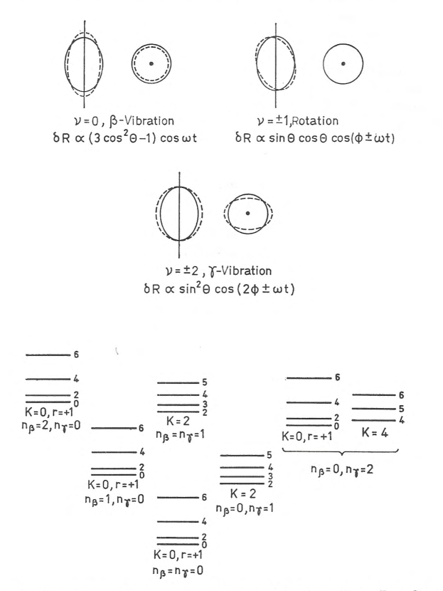
Figure 1: Various quadrupole shape oscillations in a prolate nucleus. The upper part shows projections of the nuclear shape perpendicular and parallel to the symmetry axis. The lower part shows the spectra associated with the excitation of one or two vibrational quanta including the specific values of the various oscillation energies $\hbar\omega_{\beta}$ and $\hbar\omega_{\gamma}$. The corresponding classical motion of the deviation of the surface from a sphere, $\delta R(\vartheta=\theta,\varphi=\phi,t)$ is indicated. Reproduced from [11].

2.2 The Deformed Shell Model

According to the concept of adiabaticity, the Unified Model assumes that the nucleons move in a deformed potential $v(\beta,\gamma)$ with a shape that corresponds to the instantaneous values of the slowly changing deformation variables $\beta$ and $\gamma$. The deformed single particle Hamiltonian

$$h_{def}\phi_{i}=\left(t+U(\beta,\gamma)\right)\phi_{i}=e_{i}\phi_{i},$$ (9)

generates the single particle energies $e_{i}$ and the single particle wave functions $\phi_{i}$. The most successful versions are the modified oscillator or Nilsson potential [17, 18], the Woods Saxon potential [19] and the folded Yukawa potential [20]. Because the single particle Hamiltonian $h(\beta,\gamma)$ is invariant under time reversal, it has twofold eigenstates $(i,\bar{i})$ (orbitals) with the energy $e_{i}$, which are related by time reversal. For axial potentials it has become custom to label the single particle by the Nilsson quantum numbers $[Nn_{z}\Lambda]\Omega$ of the modified oscillator potential (see [17, 6]). Respectively, they indicate the total number of oscillator quanta, the nodal number along the symmetry axis, the orbital angular momentum and the total angular momentum projections on the symmetry axis. For axial potentials the pair of time-reversed orbitals are the states with two projections $\pm\Omega$ and the same other quantum numbers.

The pair correlations are taken into account in the framework of the BCS theory by introducing the monopole pair potential $\Delta P^{\dagger}=\Delta\sum\limits_{i}c^{\dagger}_{i}c^{\dagger}_{\bar{i}}$, which generates pairs in the time reverse orbitals $(i,\bar{i})$, and $\lambda\hat{N}$, which is adjusted such that the expectation value of the particle number $\langle\hat{N}\rangle$ agrees with the actual particle number $N$. The quasiparticle Hamiltonian

$$h_{qp}=h_{def}(\beta,\gamma)+\Delta(P^{\dagger}+P)-\lambda\hat{N}$$ (10)

is diagonalized by introducing quasiparticles with the energy

$$E_{i}=\sqrt{\left(e_{i}-\lambda\right)^{2}+\Delta^{2}}.$$ (11)

The intrinsic states are configurations of excited quasiparticles with an energy equal to the sum of the quasiparticle energies, where excited states in even-$N$ nuclei have even numbers of quasiparticles and excited states in odd-$N$ nuclei have odd numbers of quasiparticles. The strength $\Delta$ of the pair potential is called the pairing gap, because it is the lowest possible quasiparticle energy. The lowest two-quasiparticle energy in even-N nuclei is larger than $2\Delta$, which generates a gap in the excitation spectrum. The lowest one-quasiparticle state, which is the ground state of the odd-$N$ neighbor, is equal or slightly larger than $\Delta$. For this reason $\Delta$ is approximately given by the energy difference between the ground state energy of the odd-$N$ nucleus and the average of the ground state energies of its two even-$N$ neighbors, which is called the even-odd mass difference $\Delta_{eo}$ (three-point even-odd mass difference). The preceding is only a sketch of the necessary rudiments of the BCS theory, which is well exposed in many textbooks, as for example in Refs.[6, 9, 22, 23, 24] and will be presented in more detail in section 3.1.

In a phenomenological approach to the Unified Model, the experimental value of the even-odd mass difference $\Delta_{eo}$ is taken to fix the pair gap $\Delta$, the deformation of the potential is determined from the experimental value of the reduced transition probability $B(E2,2^{+}_{1}\rightarrow 0^{+}_{1})$. Usually, the requirement $\langle\hat{N}\rangle=N$ places the chemical potential $\lambda$ between the last occupied and the first free level. One may allow for some adjustment of $\lambda$ to improve the agreement with the observed energies of the one-quasiparticle levels. In the following we will denote the quasiparticle configurations by $\phi(\xi)$, where $\xi$ is the short-hand notation for the nucleon coordinates with respect to principal axes of the deformed potential.

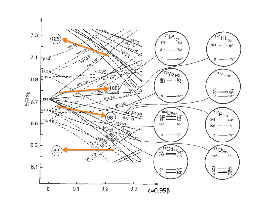
Figure 2: Single neutron orbitals in the rare earth region calculated by means of the modified oscillator potential. The circles show the position of the Fermi level for various neutron numbers. The deformation parameter $\varepsilon$ differs slightly from $\beta$ (see [6, 22]). For small deformation they are related by the indicated proportionality. The energy scale is $\hbar\omega_{0}=41A^{-1/3}$ MeV=7.5 MeV. The experimental band head energies of odd-$N$ rare-earth nuclei are shown to the right, which represent the one-quasineutron excitations. Each circle is connected with the Nilsson level pertinent to the ground state rotational band. The red arrows show how the nucleus changes its equilibrium deformation by avoiding high level density. Reproduced and modified from Ref. [22].

2.3 Deformed prolate nuclei

When the potential of the collective motion $V(\beta,\gamma)$ has a deep minimum at $\beta_{0}$ and $\gamma=0$, the deformed nuclear surface rotates and executes small-amplitude oscillations around its equilibrium shape. The resulting harmonic rotation-vibration spectrum spectrum is illustrated by the well known Fig. 1 from the monograph [6]. It is assumed that, like in molecules, the rotational frequency $\omega_{R}$ is substantially smaller than the vibrational frequencies $\omega_{\beta}$ and $\omega_{\gamma}$ and much smaller than the frequencies of the nucleons moving in the deformed potential. The different nucleonic configurations and the vibrational excitations are called the ”intrinsic states”. The mutual coupling between the intrinsic modes and the rotational mode is neglected which gives the total energy as the sum of the energies of the individual modes,

$$E=E_{ROT}+E_{int},~{}~{}E_{int}=E_{qp}+E_{V},$$ (12)

$$E_{V}=(n_{\beta}+1/2)\hbar\omega_{\beta}+(n_{\gamma}+1)\hbar\omega_{\gamma}.$$

A rotational band is built an each intrinsic state, where sequence of rotational levels is given by the eigenvalues of the rotor Hamiltonian (7). The lowest state of the band is called the band head.

The sequence of states with lowest energy at a given angular momentum is called the yrast line. The energy range up to about few MeV above the yrast line is called the yrast region. The rotational bands in this region are built on different configurations of the nucleons in the deformed rotation potential, while the vibrational modes are in the ground or the one-phonon state.

Molecules have also three different modes: rotation, vibrations of the atomic nuclei relative to each other and the motion of the valence electrons. There is a clear separation of the energy scales of the motion of the electrons and of the nuclei, which is due to the difference of their masses. As both constituents are confined to the size of the molecule,

$$\frac{\hbar\omega_{\mathrm{electronic}}}{\hbar\omega_{\mathrm{nuclear}}}\sim\frac{m_{\mathrm{nucleus}}c^{2}}{m_{\mathrm{electron}}c^{2}}\sim\frac{50000\mathrm{MeV}}{0.5\mathrm{MeV}}=10^{5}.$$ (13)

The electronic states are determined by the instantaneous potential generated by the slowly moving nuclei. The time dependence of this potential is neglected, which is called the lowest order adiabatic approximation.

The Unified Model is based on the adiabatic approximation, which is also called the strong coupling limit. It is assumed that the rotational frequency is small as compared to the typical frequencies of the nucleons in the rotating potential such that the reaction of the nucleons to the inertial forces can be neglected (or taken into account in low-order perturbation theory, see Ref. [6] 4A-3). The scale ratio for normal deformed nuclei is given by the ratio between the average splitting of the single particle levels in the deformed potential $\hbar\omega_{intrinsic}\sim\beta\hbar\omega_{0}$ (see Fig. 2) and the typical rotational transition energies $\hbar\omega_{R}=R/{\cal J}$, which is

$$\frac{\hbar\omega_{intrinsic}}{\hbar\omega_{R}}\sim\beta\hbar\omega_{0}\frac{{\cal J}}{R}\sim 0.3\times 7.4~{}\mathrm{MeV}\frac{30~{}~{}~{}}{\mathrm{MeV}~{}R}\approx\frac{60}{R}$$ (14)

at the best. The reason for the rather moderate scale ratio is that nuclei are composed of protons and neutrons that have nearly the same mass.

2.3.1 The strong coupling limit

The adiabatic approximation implies that the Hamiltonian of the Unified Model is the sum of the rotor Hamiltonian (7) and the quasiparticle Hamiltonian (10).

$$H_{UM}=H_{ROT}+H_{int},~{}~{}H_{int}=h_{qp}+H_{V},$$ (15)

where $H_{V}=T_{\beta\beta}+T_{\gamma\gamma}+C_{\beta}/2(\beta-\beta_{0})^{2}+C_{\gamma}/2\gamma^{2}$ is the vibrational part of the Bohr-Hamiltonian (6) for a potential $V(\beta,\gamma)$ that is quadratic around its minimum at $\beta_{0}$ and $\gamma=0$. The eigenstates are the product of the collective rotor wave functions and the intrinsic wave functions $\phi=\phi_{qp}\phi_{V}$ represented by the quasiparticle configurations in the deformed potential $\phi_{qp}$ and the vibrational states $\phi_{V}=\phi_{n_{\beta}}(\beta)\phi_{n_{\gamma}}(\gamma)$.

In case of molecules the well localized positions of the different atomic nuclei allows one to define the orientation of the molecule in a straightforward way. In contrast, nuclei are composed of protons and neutrons, which are identical Fermions concerning the symmetry of their many-body mean-field state in the deformed potential (see 2.2). The indistinguishability of the constituents has cutting consequences for the rotational motion, which are illustrated in Fig. 3 for the case of an axial rotor.

The collective degrees of freedom are the Euler angles which determine the orientation of the quasiparticle state $\phi(\xi)$. As illustrated by Fig. 3 (a) this intrinsic wave function is not changed by a rotation about the symmetry axis (3). The intrinsic wave function $\phi$ is an eigenfunction of $\hat{J}_{3}$, the projection of the angular momentum on the symmetry axis, with the eigenvalue $\Omega$. , The rotation operation

$${\cal R}_{3}(\varphi)\phi=\exp[-i\varphi\frac{\hat{J}_{3}}{\hbar}]\phi=\exp[-i\varphi\Omega]\phi$$ (16)

does not reorient $\phi$, because a state is only defined up to an arbitrary phase of the wave function. This means the nucleus cannot collectively rotate about the 3-axis and the moment of inertia ${\cal J}_{3}=0$. The other two moments of inertia are equal, ${\cal J}_{1}={\cal J}_{2}={\cal J}$.

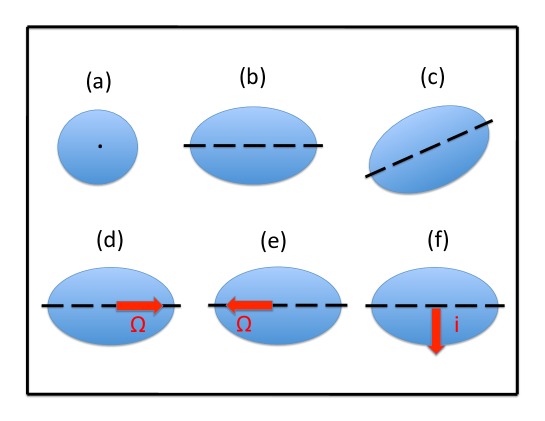
Figure 3: Rotating a prolate ensemble composed of indistinguishable particles. The red arrow indicates the angular momentum of the intrinsic state. (a): Rotating about the symmetry axis does not change the system because the constituents are indistinguishable. (b) and (c): Rotating perpendicular to the symmetry axis changes the system. (b) and (f): Rotation by $\pi$ perpendicular to the symmetry axis does not change the system. The orientation angle is restricted to one hemisphere. (d) and (e): Rotation by $\pi$ perpendicular to the symmetry axis changes the system. The orientation angles covers the full unit sphere.

The eigenvalues and eigenfunctions of the axial limit of the rotor Hamiltonian (7) are discussed in many textbooks, as e. g. [6, 9, 23, 24], which provide citations of the original work. They are given by

$$E(I)=\frac{I(I+1)-K^{2}}{2{\cal J}},~{}~{}~{}\Psi_{IMK}(\Omega)=\left(\frac{2I+1}{8\pi^{2}}\right)^{1/2}D^{I}_{M,K}(\Omega).$$ (17)

The eigenfunction are the Wigner D-functions $D^{I}_{M,K}$ which are exposed in all standard treatments of angular momentum in quantum mechanics (see e. g. Ref. [12], see also section 1A in Ref. [13] and Appendix B in Ref. [9]) . Their indices $I$, $M$, $K$, respectively, indicate the absolute angular momentum, the angular momentum projection on the laboratory z-axis and the angular momentum projection on the symmetry axis 3 in units of $\hbar$.

First we consider bands in even-even nuclei who’s intrinsic wave functions do not carry individual angular momentum along the 3-axis, i.e. $\Omega=0$. The total angular momentum agrees with the collective angular momentum of the rotor $\hat{J}_{i}=\hat{R}_{i}$ and $I=R$. The energy and the wave function of the Unified Model Hamiltonian (15) are given by

$$E(I)=E_{int}+\frac{I(I+1)}{2{\cal J}},~{}~{}~{}\Psi_{IM}(\Omega)=\left(\frac{2I+1}{8\pi^{2}}\right)^{1/2}D^{I}_{M,0}(\Omega)\phi_{K=0}(\xi).$$ (18)

It is important keeping in mind that the quasiparticle coordinates $\xi$ are defined relative to the body fixed frame of reference, that is, they change with the Euler angles $\Omega$.

As illustrated by Fig. 3 (b), rotating the intrinsic wave function $\phi$ by the angle $\pi$ about the 1-axis brings it back into an indistinguishable position, which means that it can only differ from the original one by a phase factor,

$${\cal R}_{1}(\pi)=\exp[-i\varphi\frac{\hat{J}_{1}}{\hbar}\pi]\phi=r\phi=\exp(-i\alpha\pi)\phi.$$ (19)

The phase factor $r$ or its exponent $\alpha$ are called the signature of the intrinsic state. Changing the Euler angles such that they correspond to the same rotation ${\cal R}_{1}(\pi)$ multiplies the $D^{I}_{M,0}$ functions by the phase factor $\exp(iI\pi)$, which is the phase change generated by collective rotation. To have an identical state, this phase must compensate with the phase generated by the direct rotation of $\phi$, which means that only states with $I=\alpha+2n$, $n$ integer are possible.

Each second value of $I$ is forbidden, because the symmetry of the intrinsic wave functions permits specifying the orientation of the symmetry axis only within a hemisphere. The ground state of even-even nuclei is even with respect to ${\cal R}_{1}(\pi)$, because the orbitals with $\Omega_{i}$ and $-\Omega_{i}$ are occupied with equal probability in the BCS ground state and the ground states of the vibrational modes are even as well. As a consequence, $\alpha=0$, $r=+1$ and the ground state band has only even spins. The $\beta$ vibrations have $r=1$ as well, which means that the one-phonon $\beta$ band comprises only even spins. The $K=0$ collective octupole vibration is an oscillation of a pear-shaped deformation overlaying the prolate shape. The one-phonon state has $r=-1$, which implies that the octupole band comprises only odd values of $I$.

Figs. 3 (d) and (e) illustrate the case when the intrinsic wave function carries its own angular momentum $\hbar\Omega$, which for nucleons in a non-rotating axial potential must have the direction of the symmetry axis. Since there is no collective rotation about the symmetry axis possible, the projection of the total angular momentum on the symmetry axis $K$ must be equal to the intrinsic one, $K=\Omega$. Using $\hat{J}_{1}=\hat{R}_{1},~{}\hat{J}_{2}=\hat{R}_{2},$ eigenvalues and eigenfunctions of the Unified Model Hamiltonian (15) are

$$E(I)=E_{int}+\frac{I(I+1)-K^{2}}{2{\cal J}},~{}~{}~{}\Psi_{IMK}(\Omega)=\left(\frac{2I+1}{8\pi^{2}}\right)^{1/2}D^{I}_{M,K}(\Omega)\phi_{K}(\xi),$$ (20)

where $I\geq K>0$. As seen in Fig. 3 (d,e), the presence of intrinsic angular momentum along the symmetry axis (arrow with a tip) makes it possible to specify the orientation for the whole $\Omega$ sphere, which has the consequence that there is no signature selection rule that restricts the values of $I$. The quasiparticle configurations in the axial potential are always two-fold degenerate, corresponding to the two angular momentum projections (d) and (e) in Fig. 3. They cannot be considered as two different intrinsic states because the full sphere of the possible orientations of the angular momentum arrow includes both projections in, respectively, the eastern and western hemispheres. Thus only $K>0$ should be considered as an individual intrinsic state. Care has to be taken when evaluating matrix elements with the wave functions (20) for $K=1/2$. Operators like $J_{1}$ may flip the angular momentum projection on the symmetry axis which generates matrix elements that connect the two hemispheres. In order to account for them in an explicit way, Bohr and Mottelson introduced a symmetrized version of the wave function,

$$\Psi_{IMK}(\Omega)=$$

$$=\left(\frac{2I+1}{16\pi^{2}}\right)^{1/2}\left(D^{I}_{M,K}(\Omega)\phi_{K}(\xi)+(-1)^{I+K}D^{I}_{M,-K}(\Omega){\cal R}_{2}(-\pi)\phi_{K}(\xi)\right).$$ (21)

Its form is suggested by the consideration that instead of constructing the wave function from the intrinsic configuration with the angular momentum projection pointing in the direction of the positive 3-axis, as in Eq. (20), one may also construct it from the intrinsic configuration with the angular momentum projection pointing in the direction of the negative 3-axis, which is the second term. The phase factor is derived from the requirement that the two forms must be the same wave function, including the phase. The detailed derivation can be found in the textbooks [6] (section 4.2c) and [9] (sections 6.1-6.3). As discussed in section 2.7 below, taking into account the coupling between rotation and the quasiparticle degrees of freedom in first order perturbation theory modifies the energy of the $K=1/2$ bands. The extended energy expression for all values of $K$ becomes

$$E(I)=E_{int}+\frac{1}{2{\cal J}}\left(I(I+1)-K^{2}+\delta_{K,1/2}a(-1)^{I+1/2}(I+1/2)\right).$$ (22)

The additional term splits the $K=1/2$ bands into two branches with the signatures $\alpha=\pm 1/2$, where the splitting is determined by the ”decoupling parameter” $a$.

Evaluating electromagnetic transition matrix elements, the transition operator must be transformed to the body fixed frame of reference where the integration over the intrinsic coordinates $\xi$ can be carried out. Multipole operators transform under the rotation from the laboratory coordinate system to the body-fixed system by

$${\cal M}_{\lambda,\mu}=\sum\limits_{\nu}D^{\lambda}_{\mu,\nu}(\Omega){\cal M}_{\lambda,\nu}(\xi).$$ (23)

The $\Omega$ integration over the product of the three $D$ - functions results in the product of two Clebsch-Gordan coefficients (see e. g. Ref. [12], see also section 1A in Ref. [13] and Appendix B in Ref. [9]). That is, the ratios of the electromagnetic transition matrix elements between the different members of the bands are determined by the rotational wave functions (20) only in form of the two Clebsch-Gordan coefficients. Accordingly, the reduced transition matrix elements between two bands based on the intrinsic states $\phi_{K_{f}}$ and $\phi_{K_{i}}$ are given by the Alaga rules [30]

$$\langle I_{f}K_{f}||{\cal M}_{\lambda}||I_{i}K_{i}\rangle=\left[\frac{2I_{i}+1}{(1+\delta_{K_{i}0})(1+\delta_{K_{f}0})}\right]^{1/2}\times$$

$$\{\langle I_{i}K_{i}\lambda\nu|I_{f}K_{f}\rangle\langle\phi_{K_{f}}|{\cal M}_{\lambda,\nu}|\phi_{K_{i}}\rangle$$

$$+(-1)^{I_{i}+K_{i}}\langle I_{i}-K_{i}\lambda\mu|I_{f}K_{f}\rangle\langle\phi_{K_{f}}|{\cal M}_{\lambda,\mu}|{\cal R}_{2}(-\pi)\phi_{K_{i}}\rangle\}$$

$$\nu=K_{f}-K_{i},~{}~{}\mu=K_{f}+K_{i}.$$ (24)

For transition within a band one has to use the diagonal matrix element $\langle I_{f}K_{i}||{\cal M}_{\lambda}||I_{i}K_{i}\rangle$. D. Rowe lists explicit expressions for the experimentally important electromagnetic and weak- interaction transition matrix elements in his textbook [9] (Eqs. (6.32) - (6.52) in section 6.7).

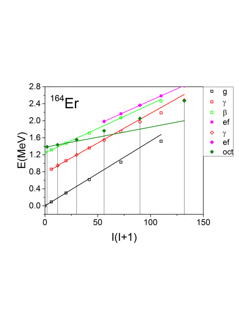
Figure 4: Experimental rotational bands in ¹⁶⁴Er. The labels indicate the bands built on the ground state (g), and on the one-phonon $\beta$, one-phonon $\gamma$, two-quasiproton (ae, af) and one-phonon octupole (oct) excitations. The convention for $(\pi,\alpha)$ is: $\pi=+$ open symbols, $\pi=-$ full symbols, $\alpha=0$ side up, $\alpha=1$ angle up. The drop lines indicate the spin value $I$. Data from Ref. [25].

2.3.2 Comparison with experiment

Fig. 4 shows the low-spin part of the rotational bands of the well-deformed nuclide ¹⁶⁴Er. The ground state band (g) has only even $I$ because the all even-even nuclei have $r=+1$. The energies follow the rigid rotor values (20) $\propto I(I+1)$ only approximately. By $I=10$ they deviate by 200 keV. Band (ef) is built on the intrinsic state that carries two excited quasiprotons, denoted by e and f. They generate an angular momentum projection of $\hbar\Omega=7\hbar$ along the symmetry axis. Even and odd values of $I$ merge into a smooth $\Delta I=1$ sequence, because the large angular momentum projection strongly breaks the ${\cal R}_{1}(\pi)$ symmetry. The moment of inertia (slope) of the band is larger than the one of the g-band. The increase is caused by a combination of weakening of pair correlations, change of deformation and modification of the microstructure of the intrinsic state.

The $\gamma$ vibration represents a deviation of the nuclear shape from axial symmetry, which travels as a wave over the nuclear surface (see Fig. 1). It carries an angular momentum of $J_{3}=\hbar K=2\hbar$ along the symmetry axis. Accordingly, the $\gamma$ band is a $\Delta I=1$ sequence. Its moment of inertia is close to the one of the g-band, which is expected for a harmonic shape vibration. This is an example for the general observation that the one-phonon $\gamma$ excitations come closest to the shape-vibrations of the Bohr Hamiltonian (see section 2.6). There is no clear evidence for harmonic the two-phonon $\gamma$ excitations.

The band denoted by $\beta$ is traditionally interpreted as the one-phonon excitation of the axial $\beta$ shape vibration, which does not carry angular momentum of its own and has $\alpha=0$. However, its structure is likely a more complex combination of the collective shape oscillation and a two-quasiparticle excitation (see section 2.6, Sec.4.4.2, the contribution to this Focus Issue by K. Heyde and J. L. Wood [7] and e. g. Ref. [26]). Accordingly, its moment of inertia differs from the one of the g-band being close to the one of the two-quasiproton band ef.

The band (oct) is based on the $K=0$ octupole vibration. It is the oscillation of a pear-shape distortion, which is odd under space inversion and odd under a rotation by $\pi$ perpendicular to the symmetry axis. Accordingly, the intrinsic state has odd parity and $\alpha=1$ and the band consists of the sequence of states with $I^{\pi}=1^{-},~{}3^{-},~{}5^{-},~{}...$. The energies strongly deviate from the rigid rotor values, which indicates that the structure of the intrinsic state changes with angular momentum.

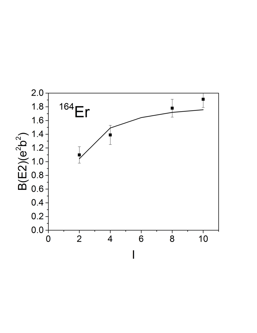
Figure 5: Reduced transition probabilities $B(E2,I\rightarrow I-2)$ for the ground state band of ¹⁶⁴Er. The line shows the axial rotor values (25) calculated with the intrinsic charge quadrupole moment $Q_{0}$=7.24 eb. Data from Ref. [27]

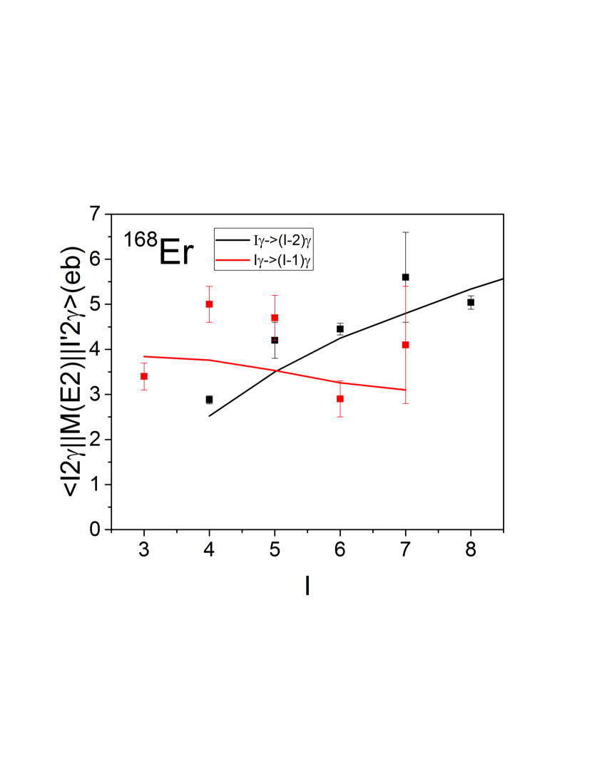
Figure 6: Reduced transition matrix elements $\langle I2,\gamma||{\cal M}_{\lambda}||I^{\prime}2,\gamma\rangle$ for transitions within the $\gamma$ band of ¹⁶⁸Er. The dashed lines (not visible) show the axial rotor values (2.3.1) calculated with the intrinsic charge quadrupole moment $Q_{0}$= 7.7 eb. The full lines show the triaxial rotor calculations. The dashed lines are not visible because two calculations are too close. Data from Ref.[28].

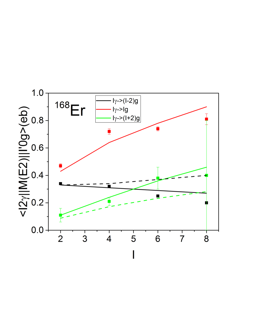
Figure 7: Reduced transition matrix elements $\langle I2,\gamma||{\cal M}_{\lambda}||I^{\prime}0,g\rangle$ for transitions between the $\gamma$ band and the ground band of ¹⁶⁸Er. The full lines show the the triaxial rotor calculations, the dashed lines the axial rotor values (2.3.1) calculated with the transition charge quadrupole moment $Q_{2}$= 0.76 eb. For $I\rightarrow I$ transitions the dashed lines are not visible because the two calculations are too close. Data from Ref. [28].

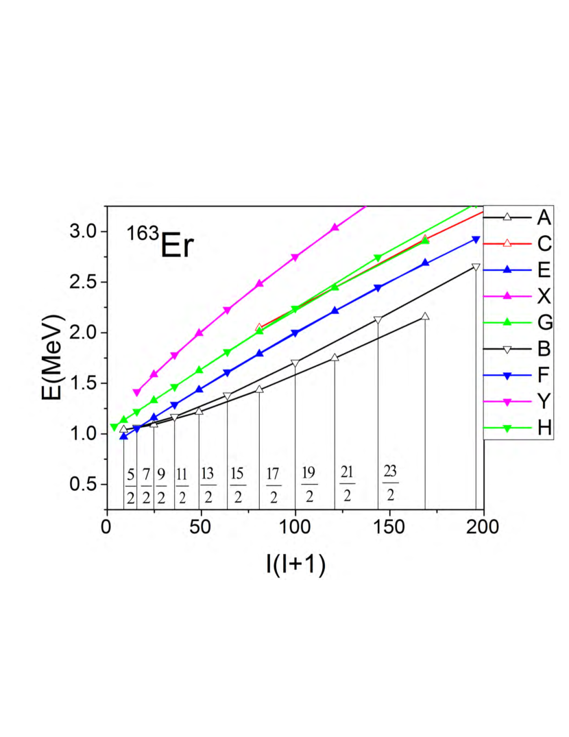
Figure 8: Experimental rotational bands in ¹⁶³Er. The labels indicate the bands built on various one-quasineutron states that are are labeled by letters. The associated Nilsson labels are quoted in Tab. 1. The convention for $(\pi,\alpha)$ is: $\pi=+$ open symbols, $\pi=-$ full symbols, $\alpha=1/2$ angle up, $\alpha=-1/2$ angle down. For consistency with later discussions the ground state has assigned an energy of 0.92 MeV, which takes into account the difference between its binding energy and the mean of the binding energies of its even-N neighbors. It represents one-quasineutron excitation energy. Seven more bands are identified with $I<7/2$ and $E^{*}<$ 0.8 MeV, which are not shown. Data from Ref. [25].

In case of the g-band of even-even nuclei the Alaga rules (2.3.1) give for the intraband transitions $I\rightarrow I-2$ the reduced transition probability

$$B(E2,I\rightarrow I-2)=\frac{5}{16\pi}\langle I~{}0~{}2~{}0|I-2~{}0\rangle^{2}e^{2}Q_{0}^{2},$$ (25)

where $eQ_{0}$ is the quadrupole moment of the prolate charge distribution as defined in [6]. Fig. 5 demonstrates that the experimental values follow closely the rigid rotor ratios

The other transition matrix elements of ¹⁶⁴Er are not well known. A good set has been extracted from the COULEX work by Kotiliński et al. [28] on ¹⁶⁸Er, which is presented in Figs. 6 and 7. (The energies follow the $I(I+1)$ rule with about the same accuracy as in ¹⁶⁴Er.) The figures show the reduced transition matrix elements (2.3.1), where the intrinsic transition matrix elements are taken as $\langle 0,g|{\cal M}_{2,0}|0,g\rangle=\sqrt{5/16\pi}Q_{0}$ and $\langle 2,\gamma|{\cal M}_{2,2}|0,g\rangle=\sqrt{5/16\pi}Q_{2}$ with $Q_{0}=7.7$ eb and $Q_{2}=0.76$ eb. The Alaga rules (2.3.1) reproduce the experiment fairly well. The $I\rightarrow I\pm 2$ transition matrix elements show systematic deviations. The detailed analysis of the similar observation in ¹⁶⁶Er by Bohr and Mottelson [6] demonstrated that the deviations are due to the coupling between the $\gamma$ and the g- band. Such a coupling can be taken into account by assuming a slight triaxiality $\gamma>0$ for the rotor Hamiltonian (7). The rotor states for small triaxiality are given in Ref. [6] (section 4.5c). Assuming that the moments of inertia depend on $\gamma$ as expected for irrotational flow (8) and that the ratio between the intrisic quadrupole moments is $Q_{2}/Q_{0}=\tan\gamma\sqrt{2}$, the $I\rightarrow I\pm 2$ transition matrix elements are well described with the choice of $\gamma=8^{\circ}$ [28]. The modification of the other matrix elements by the coupling is too small to be visible in Figs. 6 and 7. There are noticeable deviations from the triaxial rotor calculations for the $\Delta I=1$ transitions, which have a mixed E2/M1character. The M1 component is disregarded in the calculations and cannot be well extracted from the COULEX data.

The examples illustrate the general observation that the adiabatic pattern of Fig. 3 is realized in well deformed even-even nuclei for $I<10,~{}A\approx 170$ and $I<20,~{}A\approx 240$. The large gap of about 2 MeV between the ground state and the first two-quasiparticle excitations as well as the rigid shape are the reason for the adiabatic behavior. The situations is less favorite in odd mass nuclei. Fig. 8 shows the low-spin part of the rotational bands in ¹⁶³Er, which are based on different intrinsic one-quasineutron states. Fig. 2 shows that the band heads of the $N=95$ isoton ¹⁶¹Dy have quite similar energies. There is no energy gap between the ground and excited bands, because the distances between lowest quasiparticle energies $\sqrt{\left(e_{i}-\lambda\right)^{2}+\Delta^{2}}$ are strongly reduced by the pair correlations ($\Delta\sim$ 1 MeV, $|e_{i}-\lambda|\sim$0.3 MeV). The rotational bands are extracted from the dense spectrum using the fact that the intraband E2 transitions are much stronger than transitions between different bands, and that the transition energies change in a smooth way with $I$. As seen in Fig. 8, the deviations of several bands from the adiabatic $I(I+1)$ rule are substantial for some of the bands.

There is no evidence for the existence of a collective $\gamma$ vibration built on the intrinsic ground state (F). In contrast to the even-even neighbor, the collective excitation, which is expected at about 0.8 MeV, is situated among quasineutron states to which it couples. There are seven more bands identified with band heads below 0.8 MeV, which are not shown in the figure. The coupling fragments the collective mode among the states to which it couples. Studying the quasiparticle-phonon coupling experimentally requires the measurement pertinent transition matrix elements, which does not exist. Conceptually, one has reached the limit of the Unified Model.

A	$\nu[642]\frac{5}{2}$	$(+,+\frac{1}{2}$)	B	$\nu[642]\frac{5}{2}$	$(+,-\frac{1}{2}$)	C	$\nu[651]\frac{3}{2}$	$(+,+\frac{1}{2}$)
E	$\nu[523]\frac{5}{2}$	$(-,+\frac{1}{2}$)	F	$\nu[523]\frac{5}{2}$	$(-,-\frac{1}{2}$)	G	$\nu[521]\frac{3}{2}$	$(-,+\frac{1}{2}$)
H	$\nu[521]\frac{3}{2}$	$(-,-\frac{1}{2}$)	X	$\nu[505]\frac{11}{2}$	$(-,+\frac{1}{2}$)	Y	$\nu[505]\frac{11}{2}$	$(-,-\frac{1}{2}$)
a	$\pi[404]\frac{7}{2}$	$(+,+\frac{1}{2}$)	e	$\pi[523]\frac{7}{2}$	$(-,+\frac{1}{2}$)	f	$\pi[523]\frac{7}{2}$	$(-,-\frac{1}{2}$)

Table 1: Letter code used to label quasiparticle orbitals. The Nilsson labels are quoted after the letter to be followed by the parity and signature.

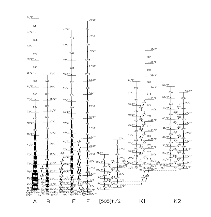
Figure 9: Partial level scheme of the nucleus ¹⁶³Er presented by Hagemann et al. [32]. The energies are given in keV. Each level is labeled by the spin and parity $I^{\pi}$. The bands are labelled by the quasiparticle configurations, which are discussed in Sects. 3.6 and 3.8.

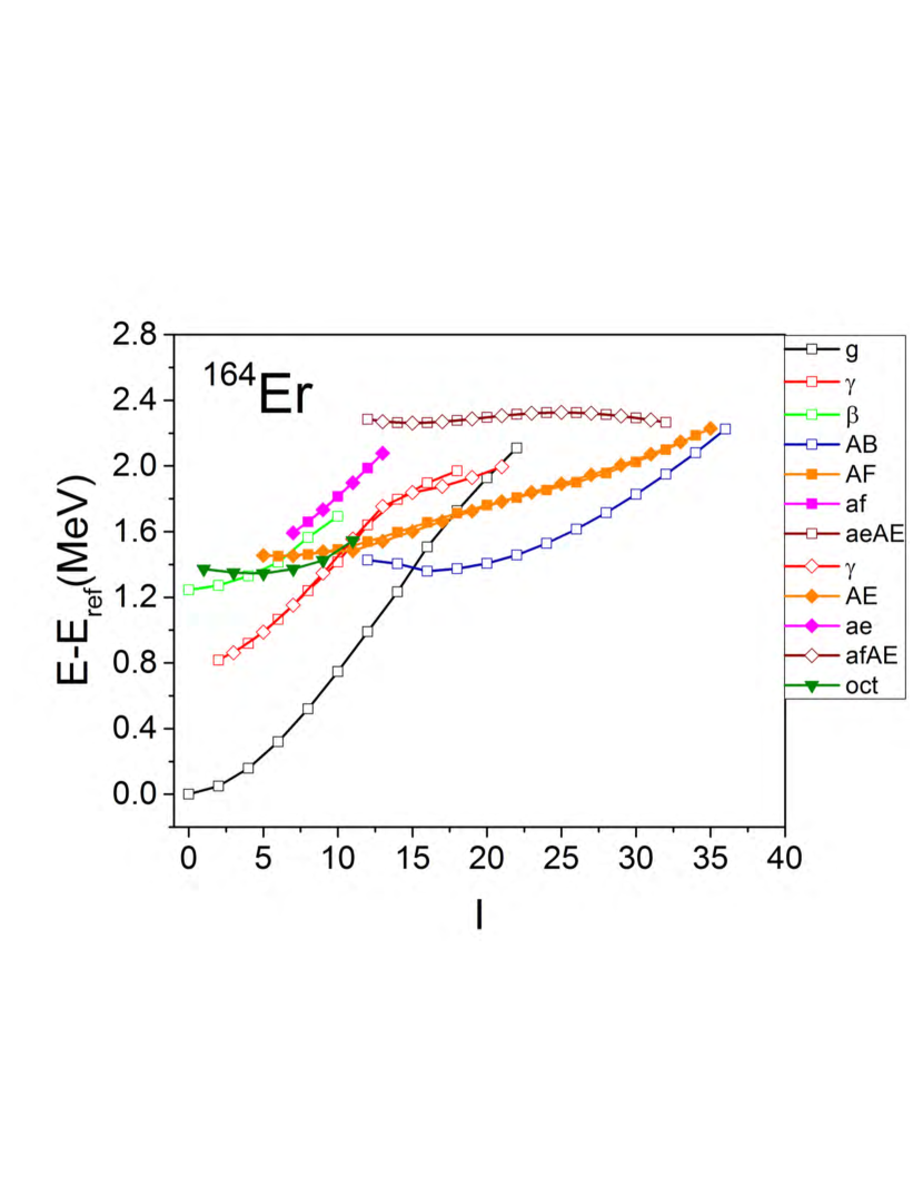
Figure 10: Experimental rotational bands in ¹⁶⁴Er. A reference energy $E_{ref}=0.007\times I(I+1)$ MeV is subtracted. The labels indicate the configuration of rotating quasiparticles. Symbol convention as in Fg. 4. Data from Ref. [25].

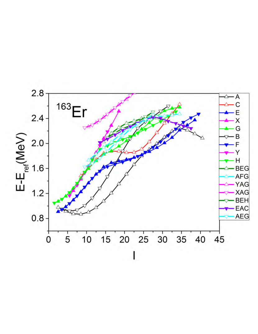
Figure 11: Experimental rotational bands in ¹⁶³Er. A reference energy $E_{ref}=0.007\times I(I+1)$ MeV is subtracted. The labels indicate the configuration of rotating quasiparticles. Symbol convention as in Fg. 8. Data from Ref. [25].

Fig. 9 shows an example of a high-spin level scheme. The transition energies between the members of a band are comparable with the energy differences between the bands, which are given by the distances between levels of the same spin. Thus differences in the energy scales cannot be used to group the levels into bands. The experimentalists arrange the measured $\gamma$ lines into a rotational spectrum like Fig. 9 as follows.
1) The states of a band are connected by fast electromagnetic transitions of low multipolarity ($E2$, $M1$, $E1$, $E3$).
2) The transition energy grows with the angular momentum $I$ in a smooth way.
3) The transition matrix elements connecting the states gradually change with $I$.
These criteria are quite handy tools for systematizing the data. However they also reflect those features of bands that remain valid at high spin. The first criterion states that the nucleus has large electromagnetic multipole moments, which are carried along with the rotation. They are the source of the radiation, which manifests itself as a cascades of sequential fast transitions. The multi-coincidence $\gamma$-detector arrays are very good filters for such cascades. The second and third criterion state that the intrinsic nuclear structure changes only gradually along a band. Figs. 10 and 11 display the energies of rotational bands up to the highest spins reached in experiment. The bands show kinks and bends which indicate major intrinsic rearrangements.

The figures illustrate the structure of the high-spin yrast region about 2 MeV above yrast line, which is the sequence of levels with minimal energy for given angular momentum. Although the energy increases by 10 MeV in the shown range of spin, the level density remains about the same in the region of about 1 MeV above the yrast line. There one can experimentally identify rotational bands and assign to them an intrinsic structure, which however is substantially modified by the inertial forces. In contrast, at zero angular momentum the same excitation energy leads into a region of very high level density (level distance eV), where one has to change to a statistical description in terms of average quantities (see Fig 16 in section 2.8).

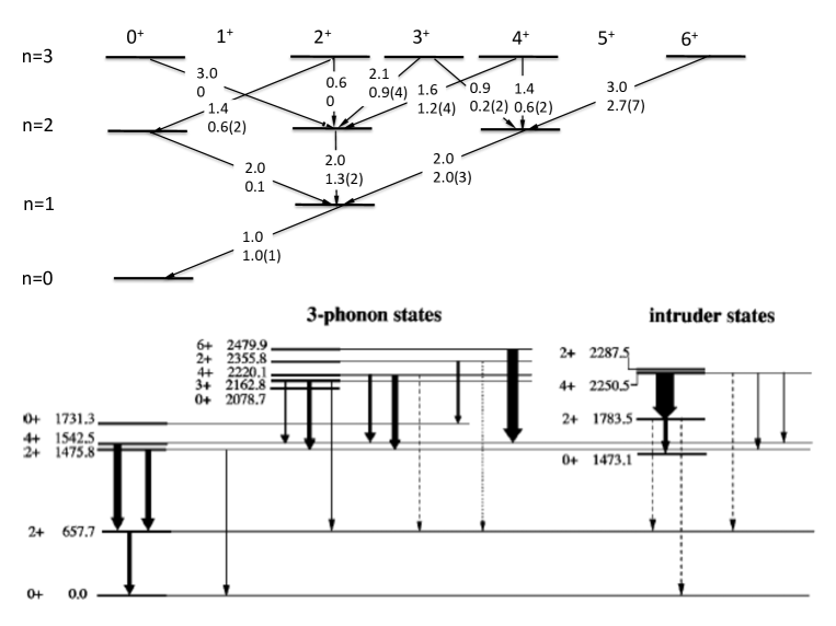
Figure 12: Upper part: The harmonic vibrator excitation spectrum. The allowed transitions are indicated by arrows. All other are forbidden. The numbers on the arrows quote the ratios of the reduced E2 transition probabilities. The upper numbers are the harmonic vibrator ratios and the lower are the experimental ratios $B(E2,I,n\rightarrow I^{\prime},n-1)/B(E2,2,1\rightarrow 0,0)$, which are taken from [33, 34, 35]. The value $B(E2,2,1\rightarrow 0,0)$=27(15) Wu from [35] is used. Lower part: The experimental levels associated with the phonon multiplets and the rotational band based on the $0_{2}^{+}$ ”intruder level”. The width of the arrows correspond to the magnitude of the experimental $B(E2)$ values. Figure is taken from Ref. [34].

2.4 Spherical nuclei

The minimum of the collective potential $V(\alpha_{\mu})$ lies at spherical shape $\alpha_{\mu}=0$. The shape executes harmonic quadrupole vibrations, which are described by the harmonic vibrator Hamiltonian

$$H_{HV}=\sum\limits_{\mu=-2}\limits^{2}(-1)^{\mu}\left[-\frac{\hbar^{2}}{2B}\frac{\partial^{2}}{\partial\alpha_{\mu}\partial\alpha_{-\mu}}+\frac{C}{2}\alpha_{\mu}\alpha_{-\mu}\right],~{}~{}\omega_{V}=\sqrt{\frac{C}{B}}.$$ (26)

It has the harmonic vibration spectrum

$$E(n)=\hbar\omega_{V}\left(n+\frac{5}{2}\right),$$ (27)

which is generated by exciting $n$ of the five degenerate phonons. The phonons are described by the operators

$$a^{\dagger}_{\mu}=\frac{1}{\sqrt{2}}\left(-b\frac{\partial}{\partial\alpha_{\mu}}+\frac{\alpha_{\mu}}{b}\right),~{}~{}a_{\mu}=\frac{1}{\sqrt{2}}\left(b\frac{\partial}{\partial\alpha_{\mu}}+\frac{\alpha_{\mu}}{b}\right),~{}~{}b=\left(\frac{\hbar^{2}}{4CB}\right)^{1/4},$$ (28)

where $b$ is the zero point amplitude. The phonon carries the angular momentum of 2$\hbar$ with the projection of $\hbar\mu$. The spectrum is composed of equidistant multiplets of $n$ phonons, which couple to the total angular momenta of $R=0$ to $R=2n\hbar$. The upper panel of Fig. 12 illustrates the spectrum and indicates the ratios between the reduced transition probabilities. For the harmonic vibrator the $B(E2)$ values increase linearly with the phonon number $n$ as long as the phonons are independently excited. Coupling them to good angular momentum redistributes the transition strength. The coefficients of fractional parentage, which determine the redistribution, are discussed in Ref. [6] (appendix 6b). The lower panel of Fig. 12 shows the lowest positive parity excitations in ¹¹⁰Cd, which is considered as one of the nuclides that come as close as possible to the harmonic vibrator limit. The $2^{+}$ one-phonon excitation lies at $\hbar\omega_{V}$=658 keV. Around 1500 keV are the three states $0^{+},~{}2^{+},~{}4^{+}$, which are interpreted as the two-phonon triplet. Their energy is about 200 keV higher than $2\hbar\omega_{V}$. The group $0^{+},~{}2^{+},~{}3^{+},~{}4^{+},~{}6^{+}$ has been associated with the three-phonon quintuplet. The experimental ratios of the yrast energies $E(I)/E(2)$= 2.3, 3.7, 5.0 for $I$=4, 6, 8 are larger than the harmonic vibrator values 2, 3, 4; their ratios $B(E2,I,n\rightarrow I^{\prime},n-1)/B(E2,2,1\rightarrow 0,0)=$1.8, 2.3 for $I=$4, 6 are smaller then the harmonic vibrator values of 2, 3 (see section 4.5). The energies of the non-yrast levels deviate from the harmonic vibrator values by comparable amounts. Their $B(E2)$ values strongly deviate from the harmonic vibrator, where the deviations increase with the distance from the yrast line. One notices that transitions that go parallel to the yrast line come closer to the harmonic vibrator values than the other. The transitions from the 0⁺ states are completely off.

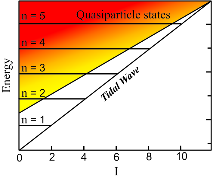
Figure 13: Schematic representation of the location of the collective quadrupole vibrational excitations relative to the quasiparticle excitations. The darker shades approximately indicate higher densities of quasiparticle states. Figure from Ref. [36].

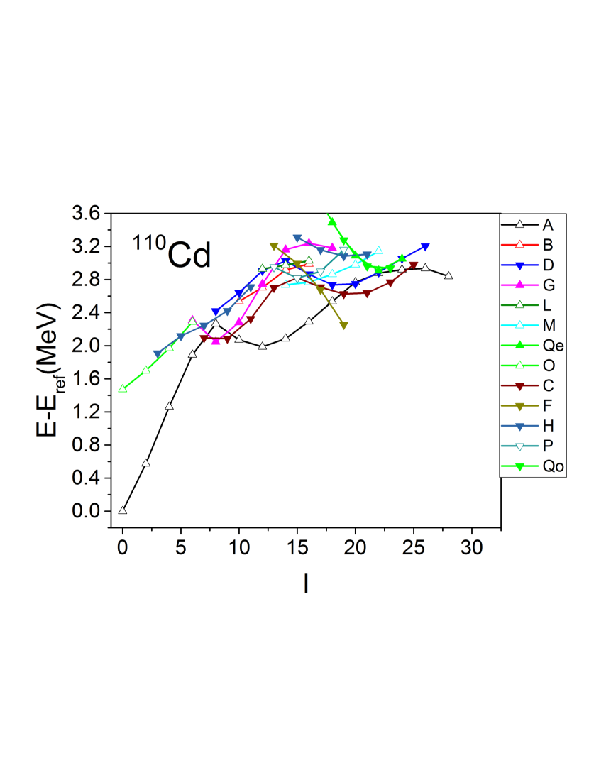
Figure 14: Experimental rotational bands in ¹¹⁰Cd. A reference energy $E_{ref}=0.014\times I(I+1)$ MeV is subtracted. The convention for $(\pi,\alpha)$ is: $\pi=+$ open symbols, $\pi=-$ full symbols, $\alpha=0$ angle up, $\alpha=1$ angle down. The parity of Qe and Qo is not known. Data from [25], from which the band labels are adopted.

The experimental spectrum contains an additional 0⁺ state upon which a rotational sequence is built. Because it does not fit into the harmonic vibrator scenario, it is often called ”intruder band”. It is the rotational band built on a deformed four quasiparticle excitation, which coexist with the harmonic vibrator spectrum built on the spherical ground state. The coexistence of the spherical shape with a deformed one is common for nuclei classified as harmonic vibrators. K. Heyde and J. L. Wood [7] discuss the shape coexistence phenomenon in great detail in their contribution to this Focus Issue.

The example describes how close real nuclei come to the harmonic vibrator spectral characteristics in general. Fig. 13 illustrates the limits of the Unified Model description of spherical nuclei in a schematic way. With increasing phonon number $n$, the zero angular momentum members of the vibrational multiplets move into the region of high density of quasiparticle excitations. The coupling to intrinsic states causes a fragmentation of the collective transition strength among an increasing number of states. The fragmentation already sets in for the $0^{+}$ state of the two-phonon triplet. The level density remains low for the yrast states of the multiplets, because of angular momentum conservation. As a consequence, the harmonic vibrator characteristics persist to higher phonon numbers. The harmonic vibrator pattern erodes with decreasing spin within a multiplet (see section 4.5).

Fig. 14 shows the yrast region of ¹¹⁰Cd up to the highest spins measured. The states can be grouped into quasi rotational sequences using the same experimental criteria as for well deformed nuclei: Strong E2 transitions connecting adjacent band members and a regular increase of $E(I)$ with $I$. The quasi rotational sequences are shorter than the rotational bands in well deformed nuclei, but the band pattern is clearly discernible. In Figs. 10, 11 and 14 an average reference energy $E_{ref}(I)=I(I+1)/2{\cal J}_{ref}$ is subtracted. The values ${\cal J}_{ref}=71\hbar^{2}$/MeV and $36\hbar^{2}$/MeV are close to the moments of inertia of rigid spheres, ${\cal J}_{rig}=2mr_{0}^{2}A^{5/3}/5$, with $A=$ 164 and 110, which are $72\hbar^{2}$/MeV and $37\hbar^{2}$/MeV, respectively. This comes not unexpected, because the yrast energy of the nucleonic Fermi gas is equal to $I^{2}/2{\cal J}_{rig}$. However, gross shell structure causes deviations of the average moment of inertia from the rigid body value [37].

2.5 Microscopic basis of the Unified Model

The preceding discussions considered the Unified Model from a phenomenological perspective. The parameters of the Unified Model, $\beta$, $\gamma$, $\Delta$, $Q_{0}$, ${\cal J}$, … were considered as adjustable to describe the experiment. The parameters can be calculated in the framework time-dependent and time-independent mean field approaches of increasing sophistication. Let us start with the potential $V(\beta,\gamma)$, which is given by the time-independent mean field. The underlying Hartree-Fock-Bogolyubov mean field theory is presented in standard textbooks on nuclear theory, as for example [9, 10, 23, 24]. Nowadays, there are four major approaches in practice, which have been refined over the last four decades such that they allow us to predict with good accuracy static properties as binding energies, radii and deformation parameters. These approaches are the shell correction method, the Skyrme energy density functional, the Gogny effective interaction and the relativistic mean field theory. A review of the immense work invested into developing these tools is beyond the focus of my contribution. Bender, Heenen and Reinhard excellently reviewed the work in 2003 [38]. For more recent developments see the literature cited in the contributions to this Focus Issue by Reinhard [39], Satula and Nazarewicz [40], Egido [41], Meng and Zhao [42] and Zhou [43].

Here I will only discuss the shell correction method [44, 45], which is also called the micro-macro approach. It over arcs the two columns of the Unified Model, the liquid drop model and the deformed shell model, in a way that allows one to calculate $V(\beta,\gamma)$ with considerable precision. It exposes the mechanism behind the appearance of stable deformation most directly and it is a time-proven simple method with predictive power that is comparable with the other selfconsistent mean field approaches being used at present. The new phenomena beyond the realm of the Unified Model, which will be discussed in this contribution, have been described in a quantitative way by the shell correction method.

Selfconsistency is the central element of the mean field approaches. The single particle orbitals, which are the eigenstates the single particle Hamiltonian $h_{def}$, generate the density matrix $\rho$. The deformed potential of $h_{def}$ is calculated from $\rho$ in different ways, which depend on the approach: Skyrme energy density functionals, the Gogny effective interaction and the relativistic mean field theory. The shell correction method uses selfconsistency only in a restricted form, which accounts for the short range of the effective nucleon-nucleon interaction. It assumes that the nuclear matter density distribution corresponds to the one of a deformed droplet, which is constant inside and drops to zero in a thin surface layer. The central single particle potential generated by the short-range interaction will have a similar profile and shape,

$$U\vec{r}~{})=\int\rho(\vec{r}~{}^{\prime})v(\vec{r},\vec{r}~{}^{\prime})d^{3}r^{\prime}~{}~{}~{}\mathrm{if}~{}~{}~{}v(\vec{r},\vec{r}~{}^{\prime})=v_{0}\delta(\vec{r}-\vec{r}~{}^{\prime})\rightarrow U(\vec{r}~{})=v_{0}\rho(\vec{r}~{}).$$ (29)

Its depth and surface thickness are parameters. The profile of the spin-orbit potential is taken as the gradient of the profile of the central potential with the strength as another parameter. The total energy is the sum of the ”macroscopic” energy of a liquid drop of nuclear matter $E_{LD}(\beta,\gamma)$ and a ”microscopic” shell correction $E_{SC}(\beta,\gamma)$,

$$E(\beta,\gamma)=E_{LD}(\beta,\gamma)+E_{SC}(\beta,\gamma).$$ (30)

Both depend on the shape, which is parametrized by a set of deformation parameters. Here we only expose the case of pure quadrupole deformation, but higher multipoles are taken into account when needed. The macroscopic liquid drop energy is the sum of a volume term, a surface term and a Coulomb term, respectively,

$$E_{LD}(\beta,\gamma)=-a_{V}\left(1-\kappa_{V}I^{2}\right)A+a_{S}\left(1-\kappa_{S}I^{2}\right)A^{2/3}B_{S}(\beta,\gamma)$$

$$+a_{C}\frac{Z^{2}}{A^{1/3}}B_{C}(\beta,\gamma),~{}~{}I=\frac{N-Z}{A},$$ (31)

where $B_{S}$ is the ratio of the surfaces areas of the deformed and the spherical droplet and $B_{C}$ is the ratio of the Coulomb energies of a homogeneously charged deformed and the spherical droplet [46]. The microscopic shell correction energy takes into account the deviations of the total energy from the macroscopic liquid drop energy due to the quantization of the nucleonic motion in the nuclear potential, which generates the shell structure. It is taken as the difference between the sum of the energies of the occupied levels $e_{i}$ of $h_{def}$ and of the levels $\tilde{e}_{i}$ of a fictitious nucleus that does not show shell structure,

$$E_{SC}=\sum\limits_{i\leq N}e_{i}-\sum\limits_{i\leq N}\tilde{e}_{i}.$$ (32)

Here, $e_{N}$ is the Fermi level, i. e. the $N^{th}$ state counting time reversed states $i$ and $\bar{i}$ explicitly. The smooth spectrum $\tilde{e}_{i}$ is obtained from the real spectrum $e_{i}$ by means of Strutinsky’s averaging procedure. It is described in Refs. [44, 45], which also derive the simple expression (30) for the total energy (see also Ref. [22]).

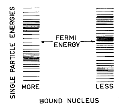
Figure 15: Qualitative illustration of the connection between the level density at the Fermi energy and the binding energy of the nucleus. Left: The occupied levels just below the Fermi energy have a smaller energy than equidistant levels with the average distance. Their contribution reduces the sum energy as compared to the sum energy of the equidistant levels. Right: The occupied levels just below the Fermi energy have a larger energy than equidistant levels with the average distance. Their contribution increases the sum energy as as compared to the sum energy of the equidistant levels. When all levels are occupied the modulation of the level density averages out. From Ref. [45]

The microscopic potential of the Bohr Hamiltonian is then given as

$$V(\beta,\gamma)=E_{LD}(\beta,\gamma)+E_{SC}(\beta,\gamma).$$ (33)

For $\gamma=0$ and up to quadratic order in the deformation parameter $\varepsilon\approx 0.95\beta$,

$$E_{LD}(\varepsilon)-E_{LD}(\varepsilon=0)=\varepsilon^{2}\left[\frac{2}{5}a_{S}\left(1-\kappa_{S}I^{2}\right)A^{2/3}-\frac{1}{5}a_{C}\frac{Z^{2}}{A^{1/3}}\right].$$ (34)

Since the liquid drop energy always prefers spherical shape, the shell energy determines the form of the potential. The shell energy is the difference of between the sum of the energies of the levels near the Fermi level and the same sum of fictitious levels with a constant average spacing. This difference is positive in regions with a level density higher than the average and negative in regions with a level density smaller than the average (see Fig. 15). That is, the maxima of $V(\beta,\gamma)$ will lie in regions of high level density and the minima in regions of low level density. This allows one to easily obtain an estimate of the equilibrium shape from a single particle energy diagram like Fig. 2. By changing its shape the nucleus tries to avoid high level density near the Fermi energy and tries to approach regions of low level density near the Fermi energy. As indicated by the red arrows in Fig. 2, the level density is low for spherical shape near the magic number $N=82$ and 126 but high for deformed shape. Somewhat away from these magic numbers the level density becomes rapidly high at spherical shape, the shell energy develops a pronounced maximum, which results in a maximum of $V(\beta,\gamma)$. There must be a minimum at deformed shape, because at large deformation the liquid drop energy prevails. The deformed minimum is stabilized by the relatively low level density for $N$ around 100, which has been called a ”deformed shell closure” in analogy to a spherical shell closure [45].

Let us now turn to the kinetic energy of the Bohr Hamiltonian. In the case of molecules, the kinetic energy of the nuclear motion is simply the sum of the kinetic energies of a set of point masses. In the case of the nuclear Unified Model one calculates the increase of the energy when the shape of the potential in the single particle Hamiltonian $h_{def}\left(\alpha(t)_{\mu}\right)$ slowly changes as a function of the five quadruple deformation parameters $\alpha(t)_{\mu}$. The kinetic energy for the Bohr Hamiltonian for the zero-quasiparticle state is obtained by solving the Schrödinger equation for the time-dependent quasiparticle Hamiltonian (10) by means of time-dependent perturbation theory, which explicitly brings in the adiabatic approximation. The energy increase caused by the collective motion is

$$T=\frac{1}{2}\sum\limits_{\mu,\nu}B_{\mu\nu}\dot{\alpha}_{\mu}\dot{\alpha}_{\nu},~{}~{}B_{\mu\nu}=2\sum\limits_{i,j}\frac{|\langle 0|\partial h_{def}/\partial\alpha_{\mu}|ij\rangle|\langle 0|\partial h_{def}/\partial\alpha_{\nu}|ij\rangle|}{\left(E_{i}+E_{j}\right)^{3}},$$ (35)

where the sum runs over all two-quasiparticle excitations $|ij\rangle$. Eq. (35) provides the generic cranking (Belyayev) expressions for the inertial parameters $B_{\mu\nu}$ used in the microscopic Bohr Hamiltonian [47]. Re-expressed in terms of the intrinsic shape parameters $\alpha_{0}=\beta\cos\gamma$ and $\alpha_{2}=\beta\sin\gamma/\sqrt{2}$ and the orientation angles, $T$ takes the form (6), where the three Inglis-Belyaev moments of inertia [48, 47]

$${\cal J}_{1,2,3}=2\sum\limits_{i,j}\frac{|\langle 0|j_{1,2,3}|ij\rangle|^{2}}{E_{i}+E_{j}}$$ (36)

appear as the inertial parameters for the angle degrees of freedom.

Kumar and Baranger [49] pioneered the microscopic calculation of the Bohr Hamiltonian and its collective wave functions in the framework of the pairing+quadrupole-quadrupole model (see section 3.1). Subsequent approaches based on the various selfconsistent mean field theories have been reviewed in Refs. [38, 15, 50, 51]. The Inglis-Belyaev expressions (35,36) well reproduce the deformation dependence of the inertial parameters. Overall, they are too small. The suppression depends on the approach but is typically of the order of 20-30%. Different ad-hoc prescriptions have been suggested to bring the mass parameters to the experimental scale, which have been used in practical calculations. When selfconsistent time-odd mean fields are taken into account, the rotational moments of inertia are changed to the Thouless-Valatin form [52], which re-produce very well the experimental values. State-dependent pairing (adding quadruple pairing to the monopole pairing as the simplest variant) generates an important contribution. This seems to indicate that using the Thouless-Valatin inertial parameters for the deformation degrees of freedom will bring them to the experimental scale. Taking the time-odd selfconsistent fields into account is still a challenging task. The contribution by K. Matsuyanagi, M. Matsuo, T. Nakatsukasa, K. Yoshida, N. Hinohara and K. Sato to this Focus Issue [51] reports progress meeting the challenge. Further developments along these lines are reviewed in Refs. [15, 50].

The quasiparticle random phase approximation (QRPA) is an alternative method to describe the vibrational excitations in a microscopic way. It can be seen as an approximation of the time-dependent mean field approach. The oscillating mean field is assumed deviating only slightly from the static equilibrium field. This allows one to linearize the equations, which then describe a harmonic vibrator. The analogy is the small-amplitude limit for a physical pendulum, which is the harmonic mathematical pendulum. The QRPA does not use the adiabatic approximation. It describes the coupling of the one-phonon vibrational excitations with the surrounding two-quasiparticle states. The QRPA is well exposed in standard textbooks on nuclear theory, as e. g. [9, 10, 23, 24]. The present status of describing the quadrupole vibrations in the framework of the QRPA will not be reviewed. Only the QRPA work on wobbling and chiral vibrations will be touched in section 3.8.5.

2.6 Transitional nuclei

The collective excitations of the nuclei in-between the well deformed and spherical limits have are described by the general solutions of the Bohr Hamiltonian (6). On the phenomenological level, the potential is parametrized by few terms of appropriate symmetry with constants that are adjusted to the experiment. The kinetic energy term is assumed to be of irrotational flow type with the overall scale as a adjustable parameter. The details have recently been reviewed by Frauendorf [15]. The virtues and limits of the Unified Model discussed for deformed and spherical nuclei appear in the transitional nuclei in the same way. The collective yrast states are best accounted for and the excited $0^{+}$ states least. Only the first excited $0^{+}$ states in nuclei located near the transition between spherical and deformed shape show the collective properties predicted by the Bohr Hamiltonian. They are particularly low in energy and have an extended wave function because of the $\beta$-flatness of the potential around the transition.

As discussed in section 2.5, the Bohr Hamiltonian has been derived microscopically in the framework of the various versions of adiabatic time-dependent mean field theory or the equivalent generator method with Gaussian approximation (see Ref. [38]). The application of the different approaches to specific nuclei has been recently reviewed Frauendorf [15]. The method, often referred to as the ”Five-Dimensional Bohr Hamiltonian” (5DBH), has considerable predictive power. Of course, it is constraint by the adiabatic approximation or the Gaussian overlap approximation. Large scale calculations of the lowest collective excitations have been carried out. In a bench mark study, Delaroche et al. [53] calculated all even-even with $10\leq Z\leq 100$ and $20\leq A\leq 200$. The results for the energies and E2 and E0 matrix elements for the yrast levels with $I\leq 6$, the lowest excited $0^{+}$ states and the two next yrare $2^{+}$ states are accessible in the form of a table as supplemental material to the publication. The authors carried out a thorough statistical analysis of the merits of performance of the method and state: ”We assess its accuracy by comparison with experiments on all applicable nuclei where the systematic tabulations of the data are available. We find that the predicted radii have an accuracy of 0.6%, much better than the one that can be achieved with a smooth phenomenological description. The correlation energy obtained from the collective Hamiltonian gives a significant improvement to the accuracy of the two-particle separation energies and to their differences, the two-particle gaps. Many of the properties depend strongly on the intrinsic deformation and we find that the theory is especially reliable for strongly deformed nuclei. The distribution of values of the collective structure indicator $R42=E(4^{+}_{1})/E(2^{+}_{1})$ has a very sharp peak at the value 10/3, in agreement with the existing data. On average, the predicted excitation energy and transition strength of the first $2^{+}$ excitation are 12% and 22% higher than experiment, respectively, with variances of the order of 40-50%. The theory gives a good qualitative account of the range of variation of the excitation energy of the first excited $0^{+}$ state, but the predicted energies are systematically 50% high. The calculated yrare $2^{+}$ states show a clear separation between $\gamma$ and $\beta$ excitations and the energies of the $2^{+},~{}\gamma$ vibrations accord well with experiment. The character of the $0^{+}_{2}$ state is interpreted as shape coexistence or $\beta$-vibrational excitations on the basis of relative quadrupole transition strengths. Bands are predicted with the properties of $\beta$ vibrations for many nuclei having R42 values corresponding to axial rotors, but the shape coexistence phenomenon is more prevalent. ” In addition the authors observe that the theory describes the $0^{+}_{2}$ states generally as too vibrational .

2.7 Quasiparticle triaxial rotor model

The quasiparticle triaxial rotor model studies a triaxial rotor to which one or more quasiparticles are coupled. Using the body-fixed frame of reference, the Hamiltonian of the coupled system is

$$H_{QTR}=H_{ROT}+h_{qp}=\sum\limits_{i=1,2,3}\frac{\left(\hat{J}_{i}-\hat{j}_{i}\right)^{2}}{2{\cal J}_{i}(\beta,\gamma)}+h_{qp}(\beta,\gamma),$$ (37)

$$=\sum\limits_{i=1,2,3}\frac{1}{2{\cal J}_{i}(\beta,\gamma)}\left(\hat{J}_{i}^{2}-2\hat{J}_{i}\hat{j}_{i}+\hat{j}_{i}^{2}\right)+h_{qp}(\beta,\gamma),$$ (38)

where $\hat{J}_{i}=\hat{R}_{i}+\hat{j}_{i}$ is the total angular momentum and $j_{i}$ the quasiparticle angular momentum. The rotor represents the collective motion of all nucleons but the explicitly treated quasiparticles. The intrinsic states are the configurations generated by combining the quasiparticles that belong to the Hamiltonian $h_{qp}$, Eq. (10). The model does not resort to the adiabatic approximation. Rather it takes fully into account the impact of the inertial forces on the quasiparticles. The coupling between the quasiparticle degrees of freedom and the rotational motion is facilitated by the ”Coriolis coupling” terms    $-\sum_{i=1,2,3}\hat{J}_{i}\hat{j}_{i}/{\cal J}_{i}(\beta,\gamma)$.

The axial rotor limit of the Unified Model, discussed in section 2.3, is recovered by setting ${\cal J}_{3}=0$ and neglecting the terms originating from $j_{1}$ and $j_{2}$, which describe action of the inertial forces on the quasiparticle motion. The wave functions (2.3.1) are the eigenfunctions and the strong coupling energies (20) are the eigenvalues of the truncated Hamiltonian. In first order perturbation theory with respect to the quasiparticle - rotation coupling the expectation value of the full Hamiltonian is taken with the unperturbed wave functions (2.3.1), which gives the energy expression (22). The signature-dependent term of the $K=1/2$ bands is the expectation value of the Coriolis coupling. The resulting expression for the decoupling parameter is

$$a=-\sum\limits_{i}\langle\phi_{K=1/2}|(j_{1,i}+ij_{2,i}){\cal R}_{2}(-\pi)|\phi_{K=1/2}\rangle.$$ (39)

The so called ”recoil term” $\sum_{i=1,2,3}\hat{j}_{i}^{2}/2{\cal J}_{i}(\beta,\gamma)$ is usually considered to be already taken into account by $h_{def}$ when fitting the deformed shell model potential to the quasiparticle levels in odd-A nuclei.

The step beyond the adiabatic limit is to diagonalize the full quasiparticle triaxial rotor model Hamiltonian (37) in the basis of the Unified Model wave functions (2.3.1) constructed from the various quasiparticle configurations. The details are laid out in the textbooks [6, 9, 22]. Limits to the number of the coupled quasiparticles are set by the dimensions of the Hamiltonian matrix but also by the Pauli Principle between the explicitly treated quasiparticles and the ones in the rotor core.

2.8 Approaches beyond the Unified Model

The territory beyond the applicability of the Unified Model depends on the direction one crosses its borderlines, and so the methods and concepts that have been developed. Fig. 13 illustrates the point for spherical nuclei and Fig. 16 for deformed. One possibility is to increase the angular momentum but stay close to the yrast line. In the yrast region, the level density remains small enough that one can study individual quantum states. The reason is angular momentum conservation, which limits the ways the excitation energy can be distributed among the nucleons. There is only one way at the yrast line, where the nucleus has ”zero temperature”. This corresponds to the well known observation that increasing the energy of a body by setting it into rotational motion does not increase its temperature (see e. g. Landau and Lifshitz Statistical Physics [29]). In the yrast region up to about 1 MeV above the yrast line, experimentalists can identify the transitions between individual states, which organize into rotational bands, or may not do so, depending on the nuclide. The rotational bands are identified by measuring multi coincidence events in large arrays of $\gamma$ ray detectors. The method and important results are discussed in the contribution to this Speccial Edition by M. A. Riley, J. Simpson and E. S. Paul [60].

The density of intrinsic states increases exponentially with the excitation energy above the yrast line. A one-to-one association of individual experimental and calculated states loses sense. One has to resort to statistical concepts as averages of energy and transition rates, their fluctuations and level densities, which implicitly invokes a certain degree of randomness that the models cannot account for. The methods of statistical mechanics have long be used for the region of excitation energies at and above the nucleon binding energy ($\sim$ 8 MeV). The computational power of modern computers has opened new avenues. The possibility to diagonalize matrices of dimension 10⁶ and more makes Shell-Model-like approaches new powerful tools. In their contribution to this Focus Issue [61], S. Leon and A. Lopez-Martens discuss ”warm nuclei”, which is the region of 2-3 MeV above the yrast line. The large density of bands and their mutual coupling require special techniques for analyzing the data from large arrays of $\gamma$ ray detectors and new concepts (rotational damping) for interpreting the $\gamma$ ray spectra emitted by these warm nuclei.

The latter path is not taken in this contribution. Rotational bands in the yrast region will be analyzed in the traditional way by comparing spectroscopic data of individual quantum states with theory. I will present work exploring the yrast region at high angular momentum, which is based on the rotating mean field approach (section 3) and the quasiparticle triaxial rotor model (section 2.7).

Important alternative developments beyond the Unified Model are left away. One example is the extensive work in the framework of the quasiparticle random phase approximation (QRPA). In their contributions to this Focus Issue, T. Nakatsukasa, K. Matsuyanagi, M. Matsuzaki and Y. R. Shimizu [54] discuss the description of vibrational excitations in rotating nuclei by means of the QRPA starting from the rotating mean field. D. R. Bes [8] and R. A. Broglia, P. F. Bortignon, F. Barranco, E. Vigezzi, A. Idini and G. Potel [55] present the Nuclear Field Theory. J. L. Egido [41] exposes the Generator Coordinate Method. The reviews [15, 50, 38] provide good citations of work on beyond-mean-field approaches.

3 Rotating mean field

The rotating mean field approach bases on the assumption that the nucleus rotates uniformly about a body-fixed axis. The time dependence is removed by transforming the theory to the frame of reference that rotates with the angular velocity $\vec{\omega}$, within which the nucleus stands still. It is known from Classical Mechanics that the Hamiltonian $H^{\prime}$ in the rotating frame is related to the Hamiltonian $H$ in the laboratory frame by the simple transformation

$$H^{\prime}=H-\vec{\omega}\cdot\vec{J},$$ (40)

where $\vec{J}$ is the total angular momentum. The transformed Hamiltonian has been called the two-body routhian [62] . The fact that $\vec{J}$ is a one-body operator leads to a dramatic simplification because it allows one to apply the mean field approximation in the same way as for the ground state. The new term $-\vec{\omega}\cdot\vec{J}$ just modifies the mean field Hamiltonian by ”cranking” it with the angular velocity $\vec{\omega}$. For this reason applying the mean field approximation to the two-body routhian (40) is also called the selfconsistent cranking model, which will be exposed in sections 3.1, 3.4.

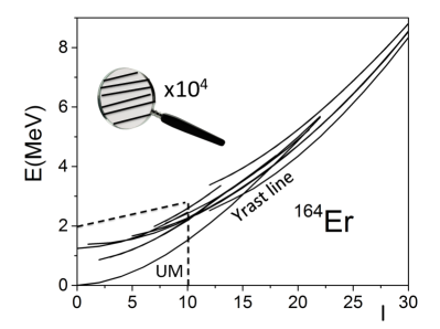
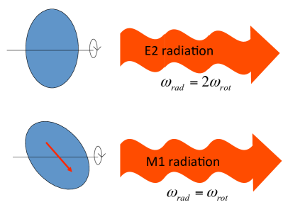
Figure 16: Left panel: Experimental energies of rotational bands in the normal deformed nucleus ¹⁶⁴Er. There are no states below the yrast line. The dashed linens delineate the realm of the Unified Model. The spacing between the rotational bands decreases exponentially with the excitation energy above the yrast line, which is illustrated by the magnifying glass. The indicated magnification factor corresponds to the location of the glass.
Right panel: Classical radiation from rotating nuclei. Upper case: The rotating charge distribution generates E2 radiation with twice the rotational frequency, because already after a half turn it returns to its original position. Lower case: The rotating magnetic moment generates M1 with the rotational frequency. The rotating charge distribution generates two kinds of E2 radiation, one with and another with $\omega_{rad}=2\omega_{rot}$.

Our focus beyond the Unified Model is on large angular momentum, for which uniform rotation about a body fixed axis can be described with good accuracy in a semiclassical way. The expressions from classical electrodynamics for radiation emission from rotating charged and magnetized bodies provide the transition matrix elements in semiclassical approximation. As illustrated by the right panel of Fig. 16, the frequency of the emitted radiation provides directly the rotational frequency $\omega$ of the nucleus. In this way, the rotational frequency can be measured by detecting the energy $\hbar\omega(E,M1)$ of the photons (cf. section 3.3). The interpretation of high-spin phenomena becomes more transparent when the angular frequency, instead of the angular momentum, is used to label the sequence of rotational states. It is useful to ”dequantize” the data, that is, to interpolate between the discrete values of the energies of the transitions connecting the rotational levels. The resulting continuous functions are directly compared with the rotating mean field calculations. This way, the multi band spectrum of the yrast region is classified in terms of configurations of quasiparticles in the rotating potential, where their response to the inertial forces is fully taken into account (sections 3.2, 3.3, 3.5, 3.6).

There is a complimentary perspective on the rotating mean field approach. Applying the mean field approximation to the two-body routhian (40 is equivalent with minimizing its expectation value with with respect to all possible mean field states. The variation

$$\delta\left(\langle H\rangle-\vec{\omega}\cdot\langle\vec{J}\rangle\right)=0$$ (41)

with respect to the quasiparticle states provides the pertinent quasiparticle routhian. The derivation is given by Ring and Schuck [23] and Blaizot and Ripka [24]. According to the Ritz Variational Principle one determines the best possible mean field state under the constraint that its expectation value of the angular momentum operator is different from zero. The mean field solutions found may have a lower symmetry than the two-body routhian, which is called spontaneous symmetry breaking. Breaking the rotational symmetry with respect to $\vec{\omega}$ axis is the prerequisite for the appearance of a rotational band. Breaking the symmetry with respect to additional discrete symmetries of the two-body routhian is reflected by different sequences of spin and parity of the band members. The discussion of the mean field symmetries in section 3.2 extends the discussion of the $\Delta=1$ and $\Delta=2$ bands in the framework of the Unified Model in section 2.3.1. The rotating mean field reveals the microscopic underpinning of the rotational degrees of freedom and has extended our view of what these are (section 4). Important new aspects are the insight that the rotating mean field may uniformly rotate about an axis titled away from the principal axes of the density distribution (section 3.8), a quantitative description of band termination (section 4.1) and the discovery magnetic rotation ((section 4.2), a new mode not anticipated in the Unified Model framework.

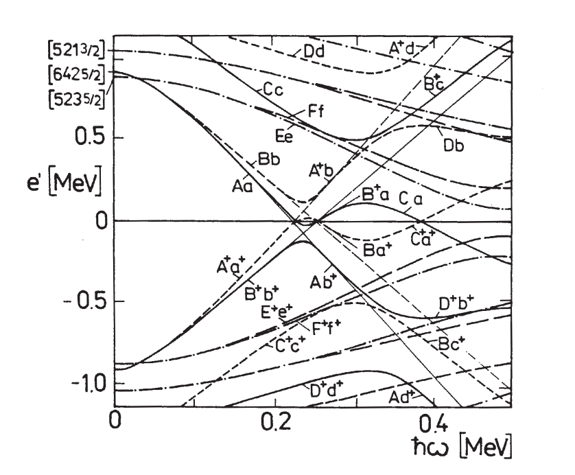
Figure 17: Quasineutron routhian trajectories for $N=96$. The figure shows the trajectories as obtained by diagonalizing the quasiparticle routhian (42) , labeled with lowercase letters, as well as the diabatic trajectories constructed from them, labeled with capital letters. The diabatic trajectories are extended through the crossings only for the levels $A,~{}B,~{}A^{+},~{}B^{+}$, where $+$ indicates the conjugate quasiparticle. Note, the frequency $\omega$ is the frequency $\omega_{1}$ discussed in the text. The figure is constructed using the parameters $\beta=0.258,~{}\Delta=0.86$ MeV. The line types indicate parity and signature $(\pi,\alpha)$: full $(+,+1/2)$, short-dashed $(+,-1/2)$, dot-dashed $(-,1/2)$, long-dashed $(-,-1/2)$. Reproduced from [71], from which the band labels are adopted.

The key assumptions -uniform rotation and semiclassics- are also the limitations of the selfconsistent cranking model. Certain phenomena are missing, like wobbling as a manifestation of non-uniform rotation with respect to the body fixed frame. Angular momentum is not conserved by the rotating mean field, which, among many other issues, leads to inaccuracies of the semiclassical transition rates or causes problems at band crossings. The quasiparticle triaxial rotor model, often used in combination with the selfconsistent cranking model, complements for these deficiencies of the rotating mean field to some extend (section 3.8.6). The Projected Shell Model (see the contributions by Y. Sun [56], P. M. Walker and F. R. Xu [57], and J. A. Sheikh, G. H. Bhat, W. A. Dar, S. Jehangir and P. A. Ganai [58] to this Focus Issue) is another approach that has been very successful in reproducing numerous spectroscopic data from the non-adiabatic regime. It starts from a set of quasiparticle configurations generated by the non-rotating mean field of the pairing + quadrupole-quadrupole Hamiltonian, generates rotational bands by projecting a sequence of states of good angular momentum from each, and finally diagonalizes a rotationally invariant Hamiltonian in the non-orthogonal basis generated this way.

3.1 Selfconsistent cranking model

The selfconsistent cranking model extends the mean field approaches from low spin to the whole yrast region. The rotational mode is treated semiclassically, which make the rotational frequency $\omega$ a central concept. The cranking term $\vec{\omega}\cdot\vec{\hat{J}}$ is subtracted from the deformed quasiparticle Hamiltonian (10),

$$h^{\prime}_{qp}(\beta,\gamma,\Delta,\lambda,\omega_{1})=h_{qp}(\beta,\gamma,\Delta,\lambda)-\vec{\omega}\cdot\vec{\hat{J}},$$ (42)

where $\vec{\hat{J}}$ is the total angular momentum operator. The cranking term describes the transformation of the quasiparticle Hamiltonian from the non-rotating frame of reference to the frame that uniformly rotates with the angular velocity $\omega$. We will refer to Hamiltonian (42) as the quasiparticle routhian. Like $h_{qp}(\beta,\gamma)$, it describes the motion of independent quasiparticles, because $\vec{\hat{J}}$ is a one-body operator. The motion in the rotating frame is subject to the inertial forces. Their strength is directly determined by the angular velocity, not the angular momentum, which is the reason for its central role of $\omega$. Compared to the microscopic Unified Model discussed in section 2.5, the new step is to take the cranking term fully into account instead of using perturbation theory. Fig. 17 shows the quasineutron routhians of an axial nucleus as functions of the frequency, which rotates about an axis perpendicular to its symmetry axis.

Conventionally (see [22, 23, 24, 31]) it was assumed that the rotational axis agrees with one of the principal axes of the deformed density distribution. Such principal axis cranking (PAC) solutions always exist. Frauendorf [87] demonstrated the existence of stable selfconsistent rotating mean field solution that uniformly rotate about an axis that is titled with respect to one of the principal axes of the deformed potential. These tilted axis cranking (TAC) solutions were only reluctantly accepted by the nuclear community, because their existence seemed to contradict basic classical mechanics, which states that a rigid body can only uniformly rotate about one of its principal axes. The origin of the tilt is discussed in section 3.8.

The elements of the selfconsistent cranking model are most transparently presented for the schematic pairing+quadrupole-quadrupole interaction [59]. The starting point is two-body routhian, which has the form

$$H^{\prime}=H_{sph}-\frac{\chi}{2}\sum\limits_{\mu=-2}^{2}Q^{+}_{\mu}Q_{\mu}-GP^{+}P-\lambda\hat{N}-\omega\hat{J}_{z},$$ (43)

where the z-axis is chosen as rotational axis. As discussed above, applying the mean field approximation to it can be seen from two complementary points of view. Interpreting expression (43) as the Hamiltonian transformed to the rotation frame of reference, its stationary mean field solutions uniformly rotate in the laboratory system, which straightforwardly leads to the semiclassical expressions for electromagnetic transition probabilities given below. Interpreting the cranking term as a constraint, the mean field solutions are the best approximation for a given finite value of the angular momentum expectation value. This complementary viewpoint is more appropriate when discussing symmetries and the nature of the rotational degrees of freedom in section 3.2.

The pairing+quadrupole-quadrupole model [59] incorporates three important aspects of the nuclear many-body system. The nucleons move in a spherical potential $U_{sph}$ with a strong spin-orbit term as the Nilsson [18] or the Woods-Saxon [19] potentials. Sometimes the energies $e_{k}$ of the levels in the spherical potential are directly adjusted to the experiment [49]. In second quantization spherical single particle Hamiltonian reads

$$h_{sph}=t+U_{sph}=\sum\limits_{k}e_{k}c^{+}_{k}c_{k},$$ (44)

where $k$ labels the single particle states.

The long range particle-hole correlations are taken into account by the second term, the quadrupole interaction. It assumed to be separable in form of a product of the quadrupole operators

$$Q_{\mu}=\sum\limits_{kk^{\prime}}\sqrt{\frac{4\pi}{5}}\langle k|r^{2}Y_{2\mu}|k^{\prime}\rangle c^{+}_{k}c_{k^{\prime}}.$$ (45)

This part of the interaction is responsible for the quadrupole deformation of the mean field.

The short range particle-particle pair correlations are taken into account by the third term, the pairing interaction. It is a product of the operators of the monopole pair field

$$P^{+}=\sum\limits_{k>0}c^{+}_{k}c^{+}_{\bar{k}},$$ (46)

were $\bar{k}$ is the time reversed state of $k$. The monopole pair field consists of Cooper pairs of protons or neutrons coupled to angular momentum zero.

The term $-\lambda\hat{N}$ controls the expectation value of the particle number $\langle\hat{N}\rangle$. To simplify the notation, the routhian (43) is written only for one kind of particles. The terms $h_{sph}$, $Q_{\mu}$ and $\hat{J}_{z}$ must be understood as sums of a proton and a neutron part and there are terms $-GP^{+}P$ and $-\lambda\hat{N}$ for both protons and neutrons.

The Hartree–Bogoliubov approximation (see [23, 24]) is used for the state vector $|\rangle$, which is an eigenstate of the mean field routhian $h^{\prime}$, which is given by

$$h^{\prime}=h_{sph}-\chi\sum\limits_{\mu=-2}^{2}q_{\mu}Q^{+}_{\mu}-\Delta(P^{+}+P)-\lambda\hat{N}-\omega\hat{J}_{z}.$$ (47)

The selfconsistency equations determine the deformed part of the potential

$$q_{\mu}=\langle Q_{\mu}\rangle,$$ (48)

the pair potential

$$\Delta=G\langle P\rangle,$$ (49)

and implicitly the chemical potential $\lambda$ by

$$N=\langle\hat{N}\rangle.$$ (50)

The quasiparticle operators

$$\alpha_{i}^{+}=\sum\limits_{k}U_{ki}c^{+}_{k}+V_{ki}c_{k}$$ (51)

obey the equations of motion

$$[h^{\prime},\alpha_{i}^{+}]=e_{i}^{\prime}\alpha_{i}^{+},$$ (52)

which define the eigenvalue equations for the quasiparticle amplitudes $U_{ki}$ and $V_{ki}$. The explicit form of these Hartree–Bogoliubov equations are given by Ring and Schuck [23] and Blaizot and Ripka [24]. The eigenvalues $e^{\prime}_{i}$ are called the quasiparticle routhians. Examples are shown in Fig. 17.

The quasiparticle operators refer to the vacuum state $|0\rangle$

$$\alpha_{i}|0\rangle=0~{}~{}\forall~{}i$$ (53)

and define the excited quasiparticle configurations

$$|i_{1},i_{2},...\rangle=\alpha_{i_{1}}^{+}\alpha_{i_{2}}^{+}...|0\rangle.$$ (54)

The construction of a configuration for a sequence of $\omega$ values, which represents a rotational band, will be discussed in section 3.6.2.

The set of Hartree-Fock-Bogoliubov equations (47)-(54) can be solved for any configuration $|\rangle=|i_{1},i_{2},...\rangle$. For such a selfconsistent solution, the total routhian

$$E^{\prime}=\langle H^{\prime}\rangle$$ (55)

has an extremum

$$\frac{\partial E^{\prime}}{\partial q_{\mu}}|_{\omega}=0,~{}~{}\frac{\partial E^{\prime}}{\partial\Delta}|_{\omega}=0$$ (56)

for the values of $q_{\mu}$ and $\Delta$ determined from the selfconsistency requirements (48,49). The total energy as function of the angular momentum is given by

$$E(J)=E^{\prime}(\omega)+\omega J(\omega),$$ (57)

$$J(\omega)=\langle\hat{J}_{z}\rangle,$$ (58)

where Eq. (58) implicitly determines $\omega(J)$. The total energy is extremal for a fixed value of $J$,

$$\frac{\partial E}{\partial q_{\mu}}|_{J}=0,~{}~{}\frac{\partial E}{\partial\Delta}|_{J}=0.$$ (59)

For a family of selfconsistent solutions $|\omega\rangle$ found for different values of $\omega$, the following canonical relations hold

$$\frac{dE}{dJ}=\omega,~{}~{}\frac{dE^{\prime}}{d\omega}=-J,~{}~{}E^{\prime}=E-\omega J.$$ (60)

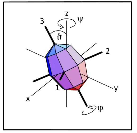
Figure 18: Euler angles specifying the orientation of the triaxial reflection symmetric density distribution. Reproduced from [14].

The calculations are most conveniently carried out in the body-fixed frame. It is the frame of the principal axes 1, 2, 3, within which the quadrupole tensor takes the simple form $q^{\prime}_{-1}=q^{\prime}_{1}=0$ and $q^{\prime}_{-2}=q^{\prime}_{2}$. Its orientation with respect to the laboratory frame is fixed by the three Euler angles $\psi$, $\vartheta$ and $\varphi$. Fig. 18 illustrates the definition of these angles. In our convention, $\psi(=\omega t)$ is the angle that grows as the nucleus rotates uniformly about the z-axis. The angles $\vartheta$ and and $\varphi$ are the orientation angles of $\vec{J}$ (i.e. of the z-axis) with respect to the principal axes . The two intrinsic quadrupole moments $q^{\prime}_{0}$ and $q^{\prime}_{2}$ specify the deformation of the potential. The quadrupole moments in the laboratory frame are related to them by

$$q_{\mu}=D^{2}_{\mu 0}(\psi,\vartheta,\varphi)q^{\prime}_{0}+(D^{2}_{\mu 2}(\psi,\vartheta,\varphi)+D^{2}_{\mu-2}(\psi,\vartheta,\varphi))q^{\prime}_{2},$$ (61)

where $D^{2}_{\nu\mu}(\psi,\vartheta,\varphi)$ are the Wigner $D$-functions .

In the body-fixed frame, the quasiparticle routhian (47) takes the form

$$h^{\prime}=h_{def}-\omega(\sin\vartheta\cos\varphi\hat{J}_{1}+\sin\vartheta\sin\varphi\hat{J}_{2}+\cos\vartheta\hat{J}_{3})$$ (62)

with

$$h_{def}=h_{sph}-q^{\prime}_{0}Q^{\prime}_{0}-q^{\prime}_{2}(Q^{\prime}_{2}+Q^{\prime}_{-2}),$$ (63)

which becomes the modified oscillator Hamiltonian when one expresses quadrupole moments by the deformation parameters

$$q^{\prime}_{0}=K\beta\cos\gamma,~{}~{}q^{\prime}_{2}=-K\beta\sin\gamma/\sqrt{2},$$ (64)

where $K=\hbar\omega_{0}/\sqrt{4\pi/5}$, $\hbar\omega_{0}=41\mathrm{MeV}/A^{1/3}$ sets the energy scale for the deformed potential. The modified oscillator Hamiltonian involves a careful parametrization of the spherical single particle energies [18].

The five selfconsistency equations (48) are reduced to two

$$q^{\prime}_{0}=\kappa\langle Q^{\prime}_{0}\rangle,\,q^{\prime}_{2}=\kappa\langle Q^{\prime}_{2}\rangle,$$ (65)

which determine $\beta$ and $\gamma$. They are complemented by the condition that $\vec{J}=\langle\hat{\vec{J}}\rangle$ must be parallel to $\vec{\omega}$ at the point of selfconsistency, which is used to determine the angles $\vartheta$ and $\varphi$. The routhian $E^{\prime}(\vartheta,~{}\varphi$) has an extremum for this orientation.

The stationarity of the eigenvalues with respect to parameter changes ensues that the negative slope of the quasiparticle routhians with respect to $\omega$,

$$i=-\frac{de^{\prime}(\omega)}{d\omega},$$ (66)

is the projection of the quasiparticle angular momentum on the rotational axis $\vec{\omega}$, which is called the aligned angular momentum or simply alignment. For example, the routhian A in Fig. 17 has the large alignment of 4.1$\hbar$.

The possible ratios between the lengths of three axes of the deformed potential are given by the values of the triaxiality parameter restricted to the interval $0\leq\gamma\leq 60^{o}$. Extending its range repeats the family of shapes with a different association of the principal axes long (l), medium (m) , short (m) with the axes labels 1, 2, 3 to which the Euler angles are attached. Tab. 2 lists the association of the 1- and 3-axes. As long as the rotational axis lies in one of the principal planes one may chose the 1-3 plane and extend the $\gamma$ interval to $-60^{o}\leq\gamma\leq 120^{o}$ to include the possible combinations m-l, s-l, s-m. Frauendorf [88] introduced this practical convention, which extends the long-practiced convention that the nucleus rotates about the 1-axis in case that the rotational axis agrees with one of the three principal axes. More details and further illustrations are given by Nilsson and Ragnasson [22] and Szymanski [31].

$\gamma$	shape	1-axis	3-axis
$-240^{o}$	prolate	short	short
	triaxial	medium	short
$-180^{o}$	oblate	long	short∗
	triaxial	long	short
$-120^{o}$	prolate	long∗	short
	triaxial	long	medium
$-60^{o}$	oblate	long	long
	triaxial	medium	long
$0^{o}$	prolate	short	long∗
	triaxial	short	long
$60^{o}$	oblate	short∗	long
	triaxial	short	medium
$120^{o}$	prolate	short	short

Table 2: Association of the semi axes of the triaxial potential with the principal axes 1 and 3. The star indicates a symmetry axis. The figure on the right illustrates the association by displaying the deformation parameters as polar coordinates, where $\beta$ is the radius and $\gamma$ the angle. It is quite common to visualize the potential energy $V(\beta,\gamma)$ and other quantities using this kind of polar coordinates, which are called the ”$\beta-\gamma-$plane”. The vertical arrows in the drawing indicate the direction of the rotational 1-axis for axial shape. For triaxial shape the axis associated with 1 is indicated by its name (the medium axis is called intermediate).

Semiclassically, the probabilities for electromagnetic transitions are given by the classical radiative power divided by the photon energy. The expressions for uniformly rotating magnetic dipoles and electric quadrupoles can be found in textbooks on classical electrodynamics, as e. g. Landau and Lifshitz Classical Fields [64]. The semiclassical transition amplitudes are proportional to the E2 and M1 multipole moments in the laboratory frame, which are related to the time-independent intrinsic moments by the transformation (23). For uniform rotation the angle $\psi=\omega t$ and for planar geometry $\varphi=0$ if rotational lies in the 1-3- principal plane (see Fig. 18). Using that $D^{\lambda}_{\mu\nu}(\psi,\vartheta,\varphi)=e^{i\mu\psi}d^{\lambda}_{\mu\nu}(\vartheta)e^{i\nu\varphi}$, the transformation (23) becomes

$${\cal M}^{lab}_{\lambda,\mu}(t)=\sum\limits_{\nu}e^{i\omega\mu t}d^{\lambda}_{\mu,\nu}(\vartheta){\cal M}^{int}_{\lambda,\nu}.$$ (67)

The expression has a straightforward meaning in classical electrodynamics, which is illustrated by the right panel of Fig. 16. The static multipole moments are given by ${\cal M}^{lab}_{1,0}(M1)$ and ${\cal M}^{lab}_{2,0}(E2)$. The multipole moments ${\cal M}^{lab}_{1,1}(M1,t)$ and ${\cal M}^{lab}_{2,1}(E2,t)$ are sources of radiation with the frequency $\omega$. The multipole moment ${\cal M}^{lab}_{2,2}(E2,t)$ is a source of radiation with the frequency $2\omega$. Using the explicit expressions for the reduced $d$ - functions given in standard textbooks on angular momentum (e. g. Ref. [12], see also section 1A in Ref. [13] and Appendix B in Ref. [9]), Frauendorf [88] derived the semiclassical transition amplitudes for the case of a planar geometry ($\varphi=0$).

The intra band M1 - transition matrix elements are

$$<I-1I-1|{\cal M}_{-1}(M1)|II>=<{\cal M}_{-1}(M1)>$$

$$=\sqrt{\frac{3}{8\pi}}\left[\mu_{3}\sin\,\vartheta-\mu_{1}\cos\,\vartheta\right].$$ (68)

The components of the transition operator ${\cal M}_{\nu}$ refer the laboratory system. The expectation value is taken with the tilted axis cranking configuration $|>$. In the second line ${\cal M}_{\nu}$ is expressed by the components of the magnetic moment in the intrinsic frame for the case that the rotational axis lies in the 1-3 principal plane. (The other three planes can be reached by extending the range of the triaxiality parameter to $-120^{\circ}\leq\gamma\leq 60^{\circ}$.) The components are related by the rotation about the Euler angle $\vartheta$ ( cf. Eq. (61), $\varphi=0$). The reduced M1-transition probability is

$$B(M1,\,I\rightarrow I-1)=<{\cal M}_{-1}(M1)>^{2}.$$ (69)

The spectroscopic magnetic moment is given by

$$\mu_{s}=<II|\mu_{z}|II>=\frac{I}{I+1/2}<\mu_{z}>$$

$$=\frac{I}{I+1/2}[\mu_{1}\sin\,\vartheta+\mu_{3}\cos\,\vartheta].$$ (70)

The factor $I/(I+1/2)$ is a quantal correction which is close to one for high spin. The components of the magnetic moment with respect to the principal axes are calculated by means of

$$\mu_{1}=\mu_{N}(J_{1,p}+(\eta 5.58-1)\,S_{1,p}-\eta 3.82\,S_{1,n}),$$

$$\mu_{3}=\mu_{N}(J_{3,p}+(\eta 5.58-1)\,S_{3,p}-\eta 3.82\,S_{3,n}),$$ (71)

where the components of the vectors of angular momentum $\vec{J}=\langle\hat{\vec{J}}\rangle$ and of the spin $\vec{S}=\langle\hat{\vec{S}}\rangle$ are the expectation values with the tilted axis cranking configuration $|\rangle$. The free spin magnetic moments are attenuated by a factor $\eta\sim 0.5-0.7$ depending on the mass region. The components of the magnetic moment can expressed as the sum of the contributions of the vacuum and the excited quasiparticles (labelled by $i$),

$$\mu_{1}=g_{R}R_{1}+\sum\limits_{i}g_{i}j_{1,i},~{}~{}\mu_{3}=g_{R}R_{3}+\sum\limits_{i}g_{i}j_{3,i},$$ (72)

where $R_{1,3}$, $j_{1,3i}$ and $g_{R}$, $g_{i}$ are the respective angular momentum components and the $g$ factors of the vacuum and of the excited quasiparticles. This form allows one to use estimates of the ingredients that are taken from experiment: Experimental $g$ factors are often known for a mass region of interest and quasiparticle angular momentum components can be derived from the spectra. Examples are the semi empirical vector models [99, 100] and [133], which will be discussed in sections 3.6, 3.8.4 (see Eqs. (105)) and 4.2, respectively.

The intra band E2 transition matrix elements are

$$<I-2I-2|{\cal M}_{-2}(E2)|II>=<{\cal M}_{-2}(E2)>=$$

$$=\sqrt{{5\over 4\pi}}\left(\frac{eZ}{A}\right)\Bigl{[}\sqrt{3\over 8}<Q^{\prime}_{0}>(\sin\,\vartheta)^{2}$$

$$+{1\over 4}<Q^{\prime}_{2}+Q^{\prime}_{-2}>\left(1+(\cos\vartheta)^{2}\right)\Bigr{]},$$

$$<I-1I-1|{\cal M}_{-1}(E2)|II>=<{\cal M}_{-1}(E2)>=$$

$$=\sqrt{{5\over 4\pi}}\left(\frac{eZ}{A}\right)\Bigl{[}\sin\,\vartheta\cos\vartheta(\sqrt{3\over 2}<Q^{\prime}_{0}>-{1\over 2}<Q^{\prime}_{2}+Q^{\prime}_{-2}>)\Bigr{]},$$ (73)

and the spectroscopic quadrupole moment is

$$Q_{s}=<II|Q_{0}^{(BM)}|II>=\frac{I}{I+3/2}<Q_{0}^{(BM)}>=$$

$$\frac{I}{I+2/3}\frac{2eZ}{A}\Bigl{[}<Q^{\prime}_{0}>\left((\cos\vartheta)^{2}-{1\over 2}(\sin\,\vartheta)^{2}\right)$$

$$+\sqrt{3\over 8}<Q^{\prime}_{2}+Q^{\prime}_{-2}>(\sin\,\vartheta)^{2}\Bigr{]}.$$ (74)

The reduced E2 transition probabilities are

$$B(E2,\,I\rightarrow I-2)=<{\cal M}_{-2}(E2)>^{2}$$ (75)

and

$$B(E2,\,I\rightarrow I-1)=<{\cal M}_{-1}(E2)>^{2}.$$ (76)

The mixing ratio is

$$\delta=\frac{<{\cal M}_{-1}(E2)>}{<{\cal M}_{-1}(M1)>}.$$ (77)

If one uses the high-spin approximation for the Clebsch-Gordan coefficients in the Unified Model one obtains the semiclassical form (3.1-77).

3.2 Symmetries

The symmetries of the two-body routhian (43) and of the mean field routhian (42) play a central role in the interpretation of the rotating mean field solutions. The symmetries are not necessarily the same. If the mean field routhian has a lower symmetry one speaks of ”spontaneous symmetry breaking”. The concept of spontaneous symmetry breaking is discussed in the textbooks [23, 24] on many-body theory of finite quantum systems. It has been conceived for phase transitions in infinite systems. When a phase has a lower symmetry than the Hamiltonian there are more than one symmetry-breaking mean field states, which all have the same energy. Their number equals the number of elements of the group of the broken symmetry. In the thermodynamic limit the symmetry breaking states become exact many-body solutions. For finite systems the exact solutions are the eigenstates of the two-body routhian, which have the same symmetry. Only approximate solutions may have a lower symmetry, which are the rotating mean field solutions. The exact eigenstates are approximated by superpositions of these degenerate rotating mean field solutions, which restore the broken symmetry . The amplitudes of such a superposition represent the collective wave function. Classifying rotating mean field solutions according to their symmetry is a fruitful concept, because the different symmetries manifest themselves clearly as the different types of rotational bands.

As discussed in the texbooks [23, 24] and section 2.3.1, breaking of the rotational symmetry with respect to the angular momentum axis leads to the appearance of a rotational band. The breaking of a discrete twofold symmetry results in the appearance of pairs of degenerate states. In a molecule the rigid localization of the atomic nuclei and the corresponding electronic wave functions break spontaneously the symmetry of the total Hamiltonian that describes the interaction between its constituents, which leads to specific degeneracies of the rotational levels. In nuclei the breaking of a two-fold symmetry by the mean field is weaker and the two states are close but not degenerate.

The order parameter is a related concept that is used for the description of phase transitions in infinite systems. An order parameter is some physical quantity that is zero in the symmetry-conserving phase and is finite in the symmetry-breaking phase. Its values distinguish between the symmetry-conserving and the symmetry-breaking states. . The spontaneous magnetization of a ferromagnet is a way to specify the different orientations of a ferromagnet, which are the degenerate symmetry-breaking states. The magnetization disappears when the temperature exceeds the critical value, where the phase transition into the isotropic paramagnetic state takes place. For finite nuclei the order parameters should specify the different orientation of the degenerate rotating mean field solutions. Suitable quantities are the magnetic dipole and electric moments, if they are large compared with a typical single-particle matrix element.

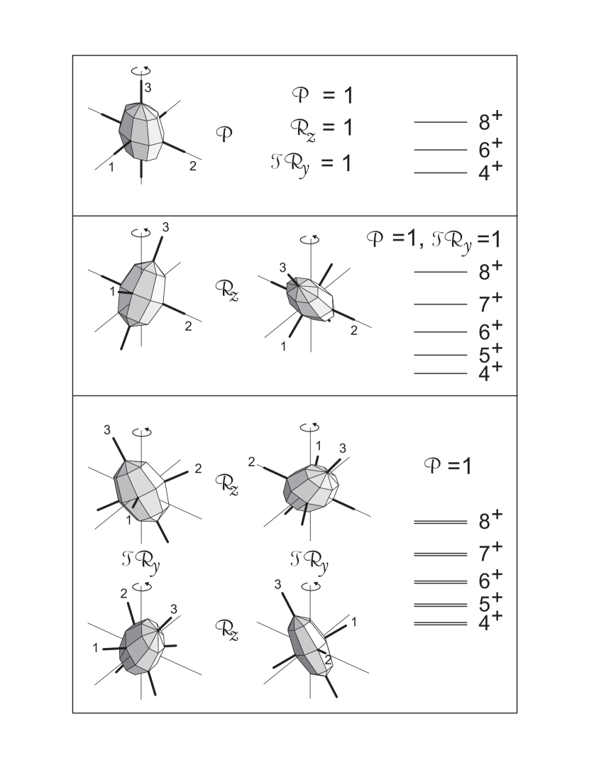
Figure 19: Discrete symmetries of the mean field of a rotating triaxial reflection symmetric nucleus (three symmetry planes). The mean field is represented by its density distribution. A polyhedron is used to make the symmetries better visible. The axis of rotation (z) is marked by the circular arrow. It coincides with the angular momentum $\vec{J}$. The figure illustrates the reorientation of the density distribution under the three symmetry operations that leave the two-body routhian invariant. The structure of the rotational bands associated with each symmetry type is illustrated on the right side.

The two-body routhian (43) is invariant with respect to

1. ${\cal R}_{z}(\psi)$, rotation about the z-axis,

2. ${\cal P}$, space inversion,

3. ${\cal R}_{z}(\pi)$, rotation about the z-axis by an angle of $\pi$,

4. ${\cal TR}_{y}(\pi)$, rotation about the x-axis by an angle of $\pi$
   combined with the time reversal ${\cal T}$.

The symmetry (iv) is a consequence of $\vec{J}$ being odd under the time reversal operation ${\cal T}$. We are interested in rotational bands, which means that symmetry (i) is broken. The symmetry operations (ii-iv) are two-fold and commute. The pairing+quadrupole-quadrupole interaction does not generate correlations that spontaneously break the space inversion symmetry. In the following it is assumed that the mean field conserves parity. The consequences of breaking the space inversion symmetry are discussed in Ref. [14].

Fig. 19 illustrates the case that the mean field routhian (47) is invariant with respect to space inversion (indicated by ${\cal P}=1$). The parity $\pi$ is a good quantum number of the mean field solutions,

$${\cal P}|\rangle=\pi|\rangle,$$ (78)

and the rotational bands are characterized by a fixed parity $\pi$. The deformed density distribution is reflection symmetric with respect to the three planes spanned by the principal axes of the quadrupole tensor (see Eq. (61)). We refer to them as the principal planes (PP) and to their intersections as the principal axes (PA). The different possible orientations of angular momentum vector $\vec{J}$ with respect to the principal axes obey the symmetries (iii) and/or (iv) or break them, which is reflected by the sequence of states in the rotational bands. The following discussion of the symmetries is not restricted to quadrupole deformations. It is valid for all shapes that have three symmetry planes (D_2h symmetry). Hexadecapole deformation is the most import reflection-symmetric deviation from quadrupole deformation. It appears in the lower region of a shell (e. g. $N\approx 90$), where nuclei look lemon-like and in the upper region (e. g. $N\approx 110$), where they look barrel-like (see e. g. [20]).

The symmetry operations ${\cal R}_{z}(\pi)$ and ${\cal TR}_{y}(\pi)$ are twofold. If the mean field is not symmetric with respect to one of them, there is for each selfconsistent solution another one with the same energy, which is generated by the symmetry operation. This follows from the invariance of the two-body routhian with respect to the symmetry operation. As a consequence, there will be two rotational bands with the same energy represented by the linear combinations of the two mean field solutions that restores the broken symmetry.

3.2.1 Axis of rotation is a principal axis

The upper panel of Fig. 19 shows the case when $\vec{J}$ has the direction of one of the principal axes (principal axis cranking - PAC). The mean field routhian $h^{\prime}$ is invariant with respect to ${\cal R}_{z}(\pi)$ and, as a consequence,

$${\cal R}_{z}(\pi)|\rangle=e^{-i\alpha\pi}|\rangle,$$ (79)

where $\alpha$ is the signature exponent or shortly the signature of the state . Since ${\cal R}_{z}(\pi)$ is a subgroup of the full rotational group, invariance of $h^{\prime}$ with respect to it leads to a selection rule for the total angular momentum,

$$I=\alpha+2n,~{}~{}n=0,\pm 1,\pm 2,....~{}.$$ (80)

The relation between the total angular momentum and $\alpha$ follows directly from the decomposition of $|\rangle$ into states of good angular momentum $|I,M=I\rangle$

$${\cal R}_{z}(\pi)|\rangle=\sum C_{I}{\cal R}_{z}(\pi)|I,M=I\rangle=e^{-iI\pi}|\rangle,$$ (81)

which implies by virtue of (79) that the sum contains only those values of $I$ that obey (80). Naturally such a wave packet is associated with a $\Delta I=2$ band according the selection rule (80).

Each quasiparticle configuration corresponds to a band of given parity and signature $(\pi,\alpha)$, i. e. to sequence of states of given parity $\pi$ and angular momentum $I$ that changes in steps of 2, in accordance with (80). The configurations with different signature have different energy. This is seen best if one connects the $\Delta I=2$ sequences of data points in a smooth way. As examples, Fig. 9 shows the two bands A and B with $(\pi,\alpha)=(+,1/2)$ and $(+,-1/2)$, which constitute two well separated $\Delta=2$ bands at large spin.

The members of the $\Delta I=2$ bands are interconnected by fast $E2$-transitions. The $\gamma$ transitions within the bands A and B in Fig. 9 are examples. The transitional quadrupole moment

$$Q_{t}\equiv Q_{22}=\sqrt{\frac{4\pi}{5}B(E2,I\rightarrow I-2)},$$ (82)

which measures the asymmetry of the density distribution with respect to the rotational axis $\vec{J}$ can be considered as the order parameter.

3.2.2 Axis of rotation in a principal plane

The middle panel of Fig. 19 shows the case when the rotational axis $\vec{J}$ is tilted away from the principal axes but still lies in one of the three principal planes (planar tilted axis cranking - planar TAC). This is always the case for axial shape. The mean field routhian is no longer invariant with respect the rotation ${\cal R}_{z}(\pi)$. Since

$${\cal R}_{z}(\pi)|\rangle\not=e^{-i\alpha\pi}|\rangle,$$ (83)

there is no restriction of $I$. The rotational bands correspond to sequences of states of all possible values of $I$ and fixed parity $\pi$. If one plots experimental energies or routhians of the states with $I=I_{o}+2n$ and $I=I_{o}+1+2n$ and connects them smoothly, the two $\Delta I=2$ sequences are degenerate, which means they combine to a $\Delta I=1$ band. In this way, the expected doubling of the number of states due to the breaking of the ${\cal R}_{z}(\pi)$ symmetry shows up. The bands K1 and K2 in Fig. 9 are examples of broken ${\cal R}_{z}(\pi)$ symmetry.

The members of the $\Delta I=1$ bands are linked by strong $E2$-transitions between the states $I$ and $I-2$ as well as by $M1$- and $E2$-transitions between the states $I$ and $I-1$. The latter are caused by the finite transitional magnetic moment $\mu_{11}\left(=\sqrt{4\pi/3B(M1,I\rightarrow I-1)}\right)$ and transitional quadrupole moment $Q_{21}\left(=\sqrt{4\pi/5B(E2,I\rightarrow I-1)}\right)$. Since both are equal to zero for ${\cal R}_{z}(\pi)$ symmetry, they may be considered as order parameters, measuring the tilt of the rotational axis or, equivalently, how strongly the ${\cal R}_{z}(\pi)$ symmetry is broken.

The preceding discussion generalizes the symmetry considerations in section 2.3.1. Within the Unified Model signature appears as a special quantum number for $K=0$ bands, because axial shape and the validity of the adiabatic approximation are assumed. More generally, the signature quantum number appears as a consequence of the symmetry mean field state under the rotation ${\cal R}_{i}(\pi)$ about one of the principal axes (see case (f) in Fig. 3). The bands A and B in Fig. 9 constitue an example. At low spin the sequences A and B combine to a $\Delta I=1$ based on $K=5/2$ intrinsic state. With increasing spin the inertial forces modify the quasiparticle state such that the $\Delta=1$ sequence splits into the two $\Delta=2$ branches with the signature $\alpha\pm 1/2$. The corresponding transition from broken to good ${\cal R}_{z}(\pi)$ symmetry will be discussed in more detail in section 3.8.5.

3.2.3 Axis of rotation out of the principal planes

The lower panel of Fig. 19 displays the aplanar tilted axis cranking case when $\vec{J}$ does not lie in one of the principal planes. Then the mean field routhian $h^{\prime}$ is no longer invariant with respect to ${\cal TR}_{y}(\pi)$, because this operation leads to a new combination of $\vec{J}$ with the system of principal axes. The two combinations have opposite chirality. To see this, first realize that the angular momentum vector $\vec{J}$ selects three principal half axes (the ones with a positive projection on $\vec{J}$). Look from the arrow head of $\vec{J}$ into this octant. Call the principal axes system right-handed if the short (1), medium (2) and long (3) axes are ordered counter clockwise (upper pair in Fig. 19) and left-handed if they are ordered clockwise (lower pair in Fig. 19). It is not possible to change the chirality by a rotation. Only the combination ${\cal TR}_{y}(\pi)$ which includes the time reversal operation ${\cal T}$ reverses the chirality.

The breaking of the ${\cal TR}_{y}(\pi)$ symmetry causes a doubling of the rotational levels. There are two identical $\Delta I=1$ sequences with the same parity, which are the even and odd linear combinations of the left- and right-handed mean field solutions. These linear combinations restore the broken ${\cal TR}_{y}(\pi)$ symmetry. The members of each band are connected by enhanced $E2$- and $M1$-transition like the planar tilted axis cranking solutions.

3.3 Rotational frequency

When the angular momentum is large it behaves almost like a classical quantity. As a consequence, the angular frequency $\omega$ also becomes a well defined observable. This presumes that we can construct a wave packet out of states with different $I$ that have otherwise similar structure, i. e. out of the members of a rotational band. At high spin it is often preferable to choose the angular frequency as the parameter that changes along the band and not the angular momentum. The modifications of the nucleonic motion are directly controlled by $\omega$, because the inertial forces depend on the angular velocity. The central role of the angular frequency in the analysis of the experimental spectra was appreciated by Bentsson and Frauendorf [62]. They introduced the experimental routhian $E^{\prime}(\omega)$, which is energy in the rotating frame of reference. It is the appropriate quantity to consider when referring to the frequency $\omega$. In classical mechanics there are the canonical relations (60) between the energy in the space-fixed and rotating frames of reference, which hold in semiclassical quantum mechanics as well. As illustrated by the right panel of Fig. 16, the rotational frequency $\omega$ is directly related to the frequency of the electromagnetic radiation which is equal to the transition energy. One may define $E^{\prime}$ and $\omega$ on the basis of the stretched quadrupole ($\Delta I=2$) or dipole ($\Delta I=1$) transitions. The choice depends on the symmetry (cf. section 3.8).

If states differing by one unit of angular momentum arrange into a $\Delta I=1$ band (e. g. the band K1 in Fig. 9) one can use

$$J=I\hbar,~{}~{}\hbar\omega(I)=E(I)-E(I-1),$$ (84)

$$E^{\prime}(I)=\frac{1}{2}[E(I)+E(I-1)]-\omega J(I).$$ (85)

Here we introduced the ”classical value” of angular momentum $J$, which can be directly compared with the results of the mean field theory.

Due to the leading order quantal correction one must associate the classical angular momentum $J$ with quantal value $I+\frac{1}{2}$. The rotational frequency $\omega$, which is defined by a transition between two rotational levels, is assigned to the mean value of $J$ of the two levels.

If states differing by two units of angular momentum arrange into a $\Delta I=2$ band (e. g. band A in Fig. 9) one must use

$$J(I)=(I-\frac{1}{2})\hbar,~{}~{}\hbar\omega(I)=\frac{1}{2}[E(I)-E(I-2)],$$ (86)

$$E^{\prime}(I)=\frac{1}{2}[E(I)+E(I-2)]-\omega(I)J(I).$$ (87)

For $\Delta I=1$ bands the rotational axis, which has the direction of the angular momentum vector $\vec{J}$, deviates from the principal axes of the nuclear shape. A majority of rotating mean field calculations assumes that the rotational axis is a principal axis. Conventionally the 1-axis is chosen. For comparison with these calculations one uses the projection $\omega_{1}$ of $\vec{\omega}$ on the principal axis 1. For axial nuclei with a substantial deformation a quite good approximation is keeping angular momentum projection on the symmetry axis $J_{3}$ constant equal to its value $K$ at the band head. The relations of classical vector geometry

$$\omega_{1}=\frac{J_{1}}{J}\omega=\frac{dJ}{dJ_{1}}\frac{dE}{dJ}=\frac{dE}{dJ_{1}},~{}~{}J_{1}=\sqrt{J^{2}-J_{3}^{2}}$$ (88)

are approximated by finite differences

$$J(I)=(I-\frac{1}{2})\hbar,~{}~{}J_{1}=\sqrt{J^{2}-(\hbar K)^{2}},~{}~{}\omega_{1}(I)=\frac{E(I)-E(I-2)}{J_{1}(I)-J_{1}(I-2)},$$ (89)

$$E^{\prime}(I)=\frac{1}{2}[E(I)+E(I-2)]-\omega_{1}(I)J_{1}(I).$$ (90)

Figs. 22 and 27 show the experimental routhians derived by means of Eqs. (89,90) from the spectrum in Fig. 9 .

The rotational frequency is a more direct experimental observable than the angular momentum, which must be constructed from the multi polarities of all the $\gamma$ transitions that form the cascade. If a certain sequence of coincident transitions is not connected with the rest of the spectrum, then one knows the frequency $\omega$ but the angular momentum only up to a constant.

Since $\omega$ changes in many small steps along a band, it is a convenient measure for studying the reaction of the nucleonic motion to the inertial forces. Choosing the rotational frequency as the band parameter facilitates the comparison with the cranking mean field theory because the latter is formulated for a given frequency. The relation (60) between the energies and the frequency, which holds exactly for the selfconsistent cranking model, ensures that the frequency used in the calculations can be identified with the experimental frequency.

Using the frequency as a rotational parameter, one distinguishes between the kinematical moment of inertia ${\cal J}^{(1)}(\omega)$ and the dynamical moment of inertia ${\cal J}^{(2)}(\omega)$ defined as

$${\cal J}^{(1)}=\frac{J}{\omega},~{}~{}{\cal J}^{(2)}=\frac{dJ}{d\omega}.$$ (91)

Authors often show experimental moments of inertia calculated from the measured energies $\Delta I=1$ transitions by means of Eqs. (84) and $\Delta I=2$ transitions by means of Eqs. (86) and, respectively,

$${\cal J}^{(1)}\left(\omega(I)\right)=\frac{J(I)}{\omega(I)},$$ (92)

$${\cal J}^{(2)}\left(\omega(I)\right)=\frac{1\hbar}{\omega(I)-\omega(I-1)}~{}~{}~{}\Delta I=1,$$ (93)

$${\cal J}^{(2)}\left(\omega(I)\right)=\frac{2\hbar}{\omega(I)-\omega(I-2)}~{}~{}~{}\Delta I=2.$$ (94)

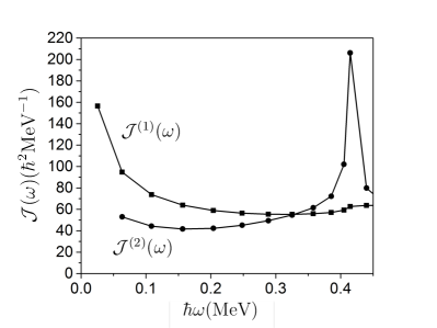
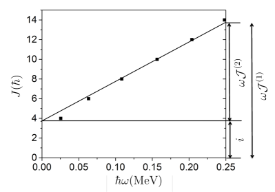
Figure 20: The experimental kinematic moment of inertia ${\cal J}^{(1)}$ and dynamic moment of inertia ${\cal J}^{(2)}$ (left) and the angular momentum $J$ (right) of band A in ¹⁶³Er calculated by means of Eqs. (86,92,94). The right panel illustrates Eq. (95), where the slight curvature of the sequence experimental points is disregarded. Data from [25].

The dynamical moment of inertia ${\cal J}^{(2)}$ measures the increment of the angular momentum with the frequency $\omega$ for a given quasiparticle configuration. It characterizes the coherent quantal states that form a rotational band. The kinematical moment of inertia ${\cal J}^{(1)}$ is a more appropriate measure for the overall increment of the energy of the states in the yrast region with angular momentum, $E(J)\approx J^{2}/(2{\cal J}^{(1)})$, irrespective of structural rearrangements.

When the adiabatic approximation is valid, the kinematic moment of inertia ${\cal J}^{(1)}$ is equal to the dynamic moment of inertia ${\cal J}^{(2)}$, and both coincide with the moment of inertia of the Unified Model. This is no longer the case when there is quasiparticle angular momentum $i$ aligned with the rotational axis. Then

$${\cal J}^{(1)}=\frac{J}{\omega}=\frac{i+{\cal J}^{(2)}\omega}{\omega}=\frac{i}{\omega}+{\cal J}^{(2)}.$$ (95)

Fig. 20 shows the band A in ¹⁶³Er as an example. Below $\hbar\omega$=0.3 MeV the dynamic moment of inertia ${\cal J}^{(2)}$ is nearly constant, because it represents the rotational response of all quasiparticles but A, which contributes an approximately constant angular momentum of $i$. The latter generates the down-slope of the in the kinematic moment of inertia ${\cal J}^{(1)}$ (see Eq. (95). A sudden increase of ${\cal J}^{(1)}$ followed by a down-slope indicate the alignment of quasiparticle angular momentum with the rotational axis. The spike of ${\cal J}^{(2)}$ at $\hbar\omega$=0.4 MeV is another signal of rapid quasiparticle alignment, which leads to a gain of $J$ without much increase of $\omega$ (see the discussion of the back bending effect in section 3.6.2). The irregularites of ${\cal J}^{(2)}$ are used as sensitive indicators of quasiparticle alignment processes. They are better visible at high frequency than the up-down in ${\cal J}^{(1)}$ (compare the feeble feature of ${\cal J}^{(1)}$ at $\hbar\omega$=0.4 MeV with the spike of ${\cal J}^{(2)}$).

Often, a more direct and practical graph is $J(\omega)$, as shown in the right panel of Fig. 20. It shows $i$ as a constant shift of the line ${\cal J}^{(2)}\omega$. As seen, the aligned angular momentum $i=3.9\hbar$ is already present at the band head. As a consequence there is no spike of ${\cal J}^{(2)}(\omega)$ that indicates the process of quasiparticle re-alignment. When the bands in the yrast region have approximately the same dynamic moment of inertia ${\cal J}^{(2)}(\omega)$ the distances between of the curves $J(\omega)$ directly provide the relative amount of angular momentum aligned with the rotational axis, which is an important information about the quasiparticle composition of the bands. The discussion of Fig. 29 in section 3.6.3 is an example.

3.4 Calculation of the mean field shape

The selfconsistent cranking approach is applied on different levels of sophistication. The simplest version is the Cranked Shell Model introduced by Bengtsson and Frauendorf [62]. It assumes that the rotational axis is the principal axis of the deformed potential with the maximal moment of inertia, which is conventially taken as the 1-axis. Its shape parameters $\beta,~{}\gamma$ and the pair potential $\Delta$ are assumed to be known. The rotational bands shown in Figs. 10 and 11 are interpreted as configurations of quasiparticles in a potential rotating with the angular velocity $\omega$. The Cranked Shell Model has become an indispensable tool for classifying the wealth of rotational bands measured with $\gamma$ ray detector arrays. It will be discussed in section 3.6.

The next level of sophistication is to calculate the quasiparticle routhian using selfconsistency. The majority of these studies assumes that the axis of rotation is a principal axis. Systematic calculations have been carried out for all versions of mean field theory. They are quite successful in reproducing rotational bands up to the highest spins. A review of this work is beyond the scope of this contribution. Only the principal axis cranking based on the shell correction method (SCPAC) introduced in Refs. [78, 79] will be presented. From the conceptual standpoint, it provides the essential new phenomena that principal axis cranking describes. The presentation is postponed to section 3.7 after discussing the properties of the quasiparticle routhians and the relation between quasiparticle configurations and rotational bands in sections 3.5 and 3.6.

Finally, the assumption that the rotational axis coincides with one of the principal axes of the density distribution is dropped. Frauendorf demonstrated the existence of selfconsistent solutions of this type, called tilted axis cranking (TAC) solutions, for the schematic pairing+quadrupole-quadrupole interaction and gave their interpretation as $\Delta I=1$ bands [87]. The tilted axis cranking approach has been laid out above for the pairing+quadrupole-quadrupole interaction, because its simplicity brings the new aspects into focus. Frauendorf [88] introduced the shell correction version of tilted axis cranking (SCTAC) and described in detail how to apply the method. Olbratowski et al. [89, 90] applied tilted axis cranking to the Skyrme density functional approach. Peng et al. [91] and Zhao et al. [92] developed tilted axis cranking for the Relativistic Mean Field approach. In their contribution to this Focus Issue, J. Meng and P. Zhao [42] describe the application of the latter to Magnetic Rotation. Tilted axis cranking will be discussed in section 3.8 with focus on its physical interpretation and symmetry aspects. A more comprehensive review, which cites the work preceding Ref. [87] and early applications, can be found in Ref. [14].

3.5 Geometry and rotational response of quasiparticle orbitals

The high-spin phenomena are governed by the balance between the cranking term $-\vec{\omega}\cdot\vec{\hat{J}}$, which favors the alignment of the quasiparticle angular momentum with the rotational axis $\vec{\omega}$ (inertial forces) and the deformed potential, which favors maximal overlap with the density distribution of a particle (nuclear interaction is short-range attractive). This interplay is particularly transparent for the ”high-j intruder orbitals” $f_{7/2},~{}g_{9/2},~{}h_{11/2},~{}i_{13/2},~{}j_{15/2}$, which are the key players in high-spin phenomena. As illustrated in in the left panel of Fig. 21, they are relatively pure spherical orbitals because the reflection-symmetric potential cannot mix them with the neighboring orbitals of opposite parity. They act like gyroscopes carrying angular momentum fixed by quantization. They favor maximal overlap of their torodial density distribution with the deformed potential. Away from this orientation, the torque causes a precession motion. For axial shape a particle tends to align its angular momentum with the axis perpendicular to the symmetry axis, because this orientation corresponds to maximal overlap with the attractive potential. A hole prefers an orientation that minimizes the overlap of its density with the deformed potential, which is repulsive for a hole. Accordingly it tends to align with the symmetry axis. For triaxial shape a particle tends to align with the short axis, because this orientation maximizes the overlap, whereas a hole tends align with the long axis the long axis, minimizing the overlap.

The interplay between the torque excerted by the deformed potential and the inertial forces result in different coupling schemes, which are illustrated in Fig. 21 by means of the precession cone carried out by the angular momentum vector of the quasiparticle [67]. The figure also shows the fingerprint of the coupling scheme in a quasiparticle diagram like Fig. 17.

At low frequency the torque exerted by the deformed potential causes $\vec{j}$ to precess around the symmetry axis 3, i. e. $\langle j_{1}\rangle=i\approx 0$ and $\langle j_{3}\rangle\approx\hbar\Omega$, the quantized angular momentum projection on the symmetry axis without rotation. The trajectories of the routhians are horizontal and degenerate with respect to the signature $\alpha$. The coupling scheme is called deformation aligned (DAL) because the precession cone is aligned with the symmetry axis of the potential. In this context ”aligned with the axis” means that the axis is located within the cone. Of course, DAL is the coupling scheme of the adiabatic limit of the Unified Model.

At large frequency the inertial forces prevail, which cause $\vec{j}$ precessing about the 1-axis, i. e. $\langle j_{1}\rangle=i\approx const$ and $\langle j_{3}\rangle\approx 0$. The precession angle is given by the quantization of $j_{1}=\hbar m$. The trajectories of the routhians have a constant slope $-\hbar m$ and are ordered according to the energy $-\hbar\omega m$ with alternating signature $\alpha=m+2n$. This coupling scheme is called rotation aligned (RAL) because the precession cone is aligned with the rotational axis.

For the lowest quasiparticles the pair field generates a tendency toward RAL. The superposition of particle and hole components, which have opposite quadrupole moments, reduces the net quadrupole moment of the quasiparticle and thus its coupling to the deformed potential. A new coupling scheme appears. It corresponds to precession about an axis $\vec{j}_{\lambda}$, which has the angle $\arccos[j_{3\lambda}/j]$ with the 3-axis, where $j_{3\lambda}$ is the angular momentum projection of the Fermi level on the symmetry axis. Both $j_{3\lambda}$ and $i$ are approximately constant. The fingerprint corresponds to constantly sloping trajectories, which are degenerate with respect to the signature $\alpha$. The scheme has been called Fermi aligned (FAL) because the precession cone is aligned with the $\vec{j}_{\lambda}$ axis that lies on the precession cone of the Fermi level [67].

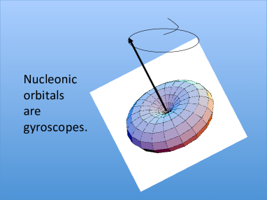
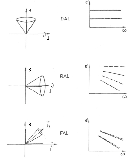
Figure 21: Left panel: Density distribution and angular momentum of a high-j orbital (f_7/2, g_9/2, h_11/2, i_13/2, j_15/2). They remain relatively pure spherical orbitals because the deformed reflection-symmetric nuclear potential does not mix them with the surrounding orbitals of opposite parity. Its torque causes a precession motion. Right panel: The three coupling schemes for a nucleus rotating about an axis perpendicular to its symmetry axis and their fingerprints in the quasiparticle routhian trajectories.

The semiclassical analysis in A provides a more detailed picture of the coupling of high-j orbitals with the triaxial potential, which extends the work in Refs. [65, 66, 67, 68, 69].

Frauendorf [88] also analyzed how the normal parity quasiparticles couple to the deformed rotating potential. In the case of a prolate axial deformation the orbitals with a large projection $j_{3}$ are strongly coupled to the deformed potential. They have the same $-j_{3}\omega\cos\vartheta$ dependence discussed above for the hole type high-$j$ orbitals. The states originating from low-$K$ Nilsson levels show a complex behavior, which cannot be explained in a simple way. An exception are the pseudo spin singlets, which will be briefly discussed in section 3.8.3.

In summary, the fingerprint for RAL coupling is a well-split sequence of states of alternating signature with approximately constant aligned angular momentum $i=\langle j_{1}\rangle=-de^{\prime}/d\omega$, which decreases with energy. The fingerprints of DAL coupling are signature doublets with finite angular momentum aligned with the deformation axis and no (or small negative) angular momentum aligned with the rotation axis. The fingerprint of FAL coupling are signature doublets with with finite angular momentum aligned with the deformation axis and substantial angular momentum aligned with the rotation axis.

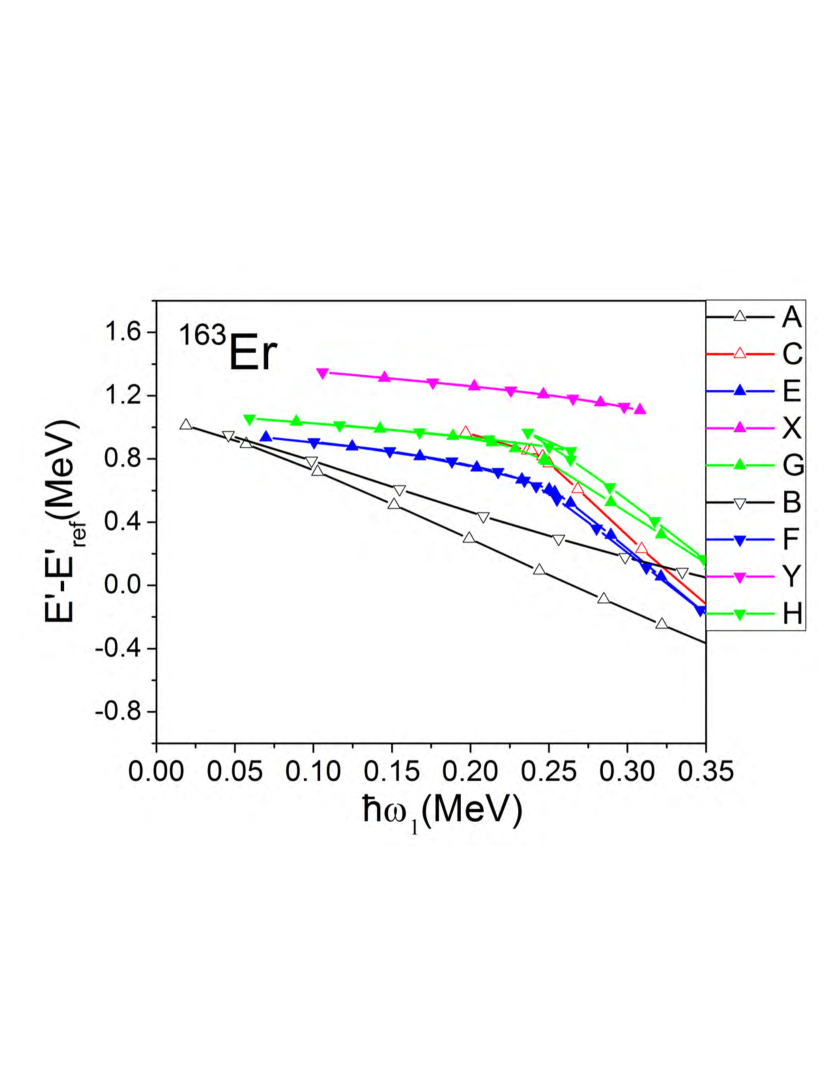
Figure 22: Experimental routhians in ¹⁶³Er relative to the g-band reference routhian $E_{ref}$. The symbol convention is the same as in Fig. 4. The routhians are calculated by means of Eqs. (89,90), where $K=5/2$ is used for A, B, E, F, and $K=11/2$ for X, Y. Configurations involving quasiprotons and several three-quasineutron configurations are left away for clarity. Data from Refs. [25] and [32], from which the band labels are adopted.

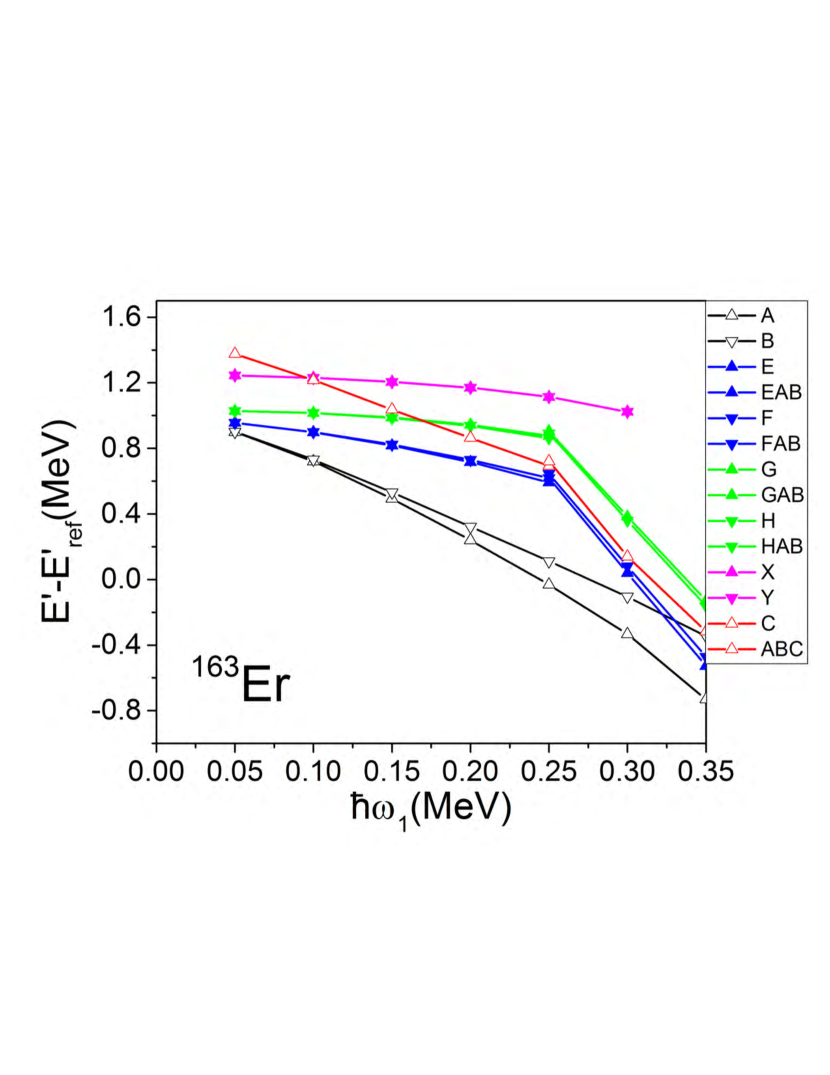
Figure 23: Calculated routhians in ¹⁶³Er relative to the calculated g-band reference routhian $E_{ref}$. Symbol convention as in Fig. 4. Configurations involving two-quasiproton and several three-quasineutron configurations are left away for clarity.

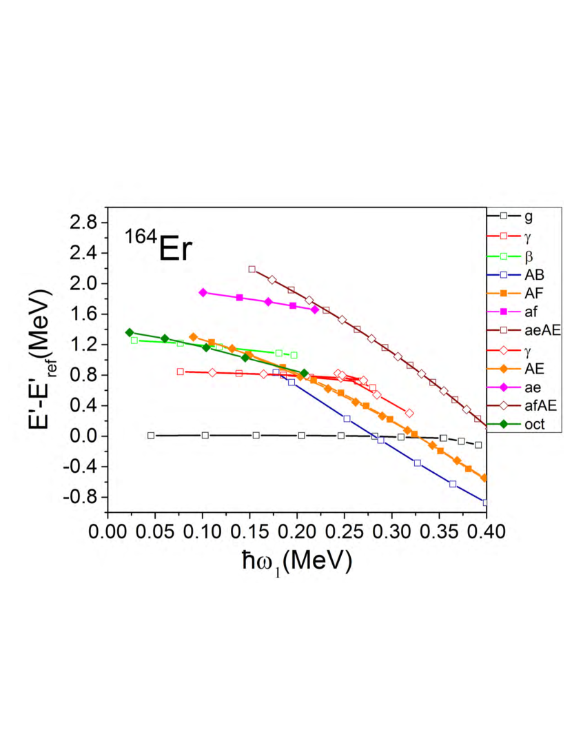
Figure 24: Experimental routhians in ¹⁶⁴Er relative to the g-band reference routhian $E_{ref}$. The symbol convention is the same as in Fig. 4. Data from Ref. [25] from which the band labels are adopted. The routhians are calculated by means of Eqs. (89,90), where $K=0$ is used for g, AB; $\beta$, oct; $K=2$ for $\gamma$; $K=5$ for AE, AF; $K=7$ for ae, af; and $K=12$ for aeAE, afAE.

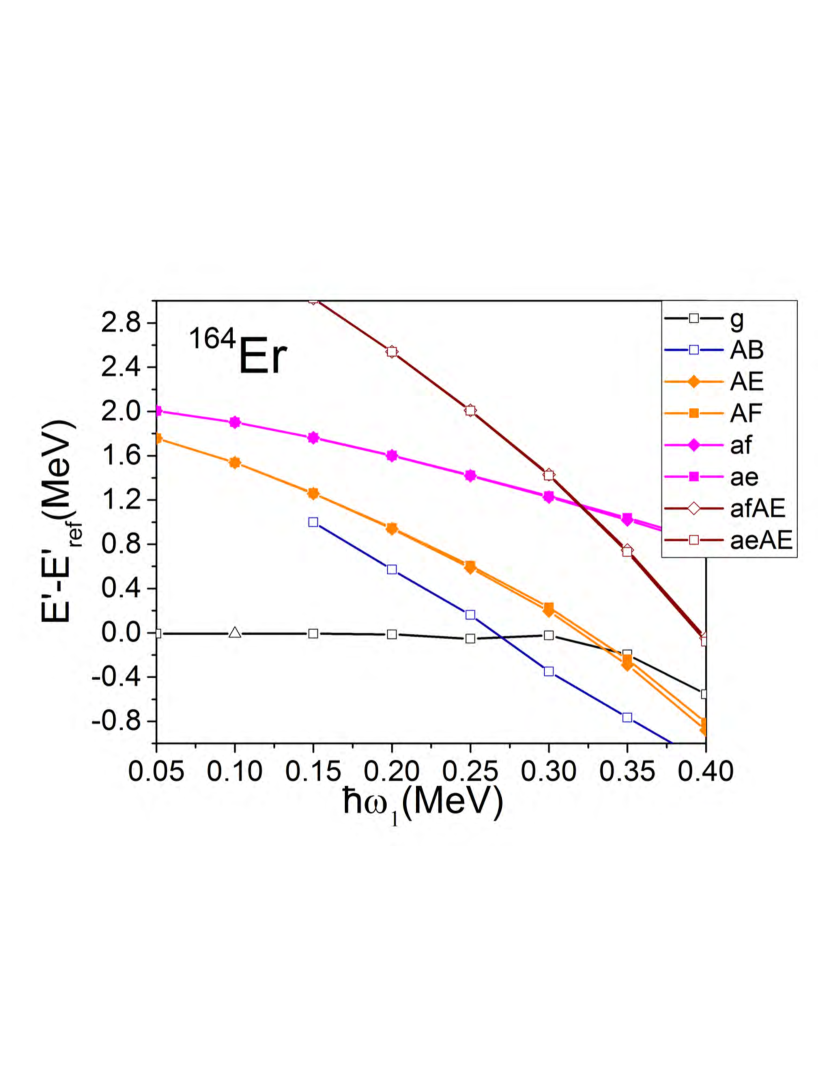
Figure 25: Calculated routhians in ¹⁶⁴Er relative to the calculated g-band reference routhian $E_{ref}$. The symbol convention is the same as in Fig. 4.

3.6 Cranked Shell Model

The concept of the Cranked Shell Model was established by Bengtsson and Frauendorf [62]. A detailed presentation was given by Bengtsson, Frauendorf and May [71], which contains a collection of quasiparticle routhians. In the spirit of the conventional Shell Model it considers configurations of independent nucleons which occupy the eigenstates of the single particle routhian

$$h^{\prime}(\beta,\gamma,\omega_{1})\phi_{i}=\varepsilon^{\prime}_{i}(\beta,\gamma,\omega_{1})\phi_{i},~{}~{}~{}h^{\prime}(\beta,\gamma,\omega)=h(\beta,\gamma)-\omega_{1}j_{1}$$ (96)

according to the Pauli principle. The energies in the rotating frame of reference, $\varepsilon^{\prime}_{i}(\beta,\gamma,\omega)$, are called the single particle routhians. The single particle routhian operator (96) conserves parity. In addition it is invariant with respect to a rotation by $\pi$ about the 1-axis, which implies that its eigenstates carry the signature quantum number $\alpha$,

$${\cal R}_{1}(\pi)\phi_{i}=e^{-i\pi\alpha_{i}}\phi_{i},~{}~{}~{}\alpha=\pm 1/2.$$ (97)

The total parity is the product of the single particle parities. The total signature $\alpha$ of a configuration is the sum of the single particle signatures, which is related to the angular momentum of the band by $I=\alpha+2n$ for the same reason as discussed for the Unified Model above. As usual, the relative energies of the various configurations are equal to the differences between the sums of the routhians of all occupied states, provided the deformation parameters and the angular frequency $\omega_{1}$ are the same. This means the bands can be classified as the particle-hole configurations in the same way as for the non-rotating deformed potential of the Unified Model. The simplicity only reveals when one compares routhians at a given frequency $\omega_{1}$.

The particle-hole scheme works only at sufficiently high spin, where the pair correlations can be neglected. In their contribution to this Focus Issue [60], M. A. Riley, J. Simpson and E. S. Paul present the Cranked Shell Model interpretation of the rotational bands ^{159,160,161,162}Er. For $\hbar\omega>0.4$MeV the experimental routhians can be surprisingly well reproduced as particle-hole configurations of single particle routhians.

At moderate spin, where the pairing correlations must be taken into account, one must change to quasiparticle configurations. The quasiparticle routhians are found by diagonalizing the double-dimensional quasiparticle routhian (42). The details are given e. g. in Ref. [62] or the in the textbooks nuclear many body theory [23, 24]. The quasiparticle routhians $e_{i}^{\prime}$ appear in the symmetric way shown in Fig. 17. At low spin the quasiparticles simply occupy the solutions $e_{i}>0$. When the quasiparticle routhians cross with zero the interpretation simplifies using an extended occupation scheme that includes the $e_{i}<0$ part. The modified rules state that

• One half of all quasiparticle routhians is occupied and the conjugate half is free.

• Out of a conjugate pair only one of the re-occupied states contributes to the change of energy, aligned angular momentum, signature, parity and other quantities.

The second rule is meant for the Cranked Shell Model only, which calculates energy differences between quasiparticle configurations for fixed mean-field parameters. The excitation energies are taken relative to some reference configuration, which may be chosen differently depending on the spin range.

The reference routhian and angular momentum can be well approximated by the Harris expressions

$$J_{1ref}=i_{r}+\omega\Theta_{0}+\omega^{3}\Theta_{1},~{}~{}E_{ref}=e_{r}+i_{r}\omega+\frac{\omega^{2}}{2}\Theta_{0}+\frac{\omega^{4}}{4}\Theta_{1}+\frac{\hbar^{2}}{8\Theta_{0}}.$$ (98)

For low and moderate spin the natural choice is the ground state (g-) band of the even-even nucleus, which has $i_{r}=e_{r}=0$. For our example ¹⁶⁴Er, the experimental energies of the g-band give $\Theta_{0}=32\hbar^{2}$MeV^-1 and $\Theta_{1}=32\hbar^{4}$MeV ^-3. This reference is subtracted in Figs. 22, 24 and 29. The experimental relative routhians are compared with the calculated ones in Figs. 23 and 25 . The parameters of the Cranked Shell Model reference are adjusted to the calculated routhian of the g-configuration.

3.6.1 Bands as quasiparticle configurations

Fig. 17 shows the quasineutron routhians for $N\approx 96$. A collection of such quasiparticle diagrams for the rare earth region can be found in Ref. [71]. The quasiparticle trajectories are classified by means of the parity and signature, $(\pi,\alpha)$. The different rotational bands correspond to the various possibilities of occupying the quasiparticle levels, i. e. to quasiparticle configurations. The large number of bands identified with multi $\gamma$ ray detector arrays necessitates a compact notation. A letter is assigned to each quasiparticle, where the convention is used that the first letters of the alphabet A, B, C, D are used for the high-j intruder states (i_13/2 neutron in our example) and E, F, G, …. for the normal parity states. For the discussion we use the letter code of Fig. 17 and its extension in Table. 1.

The vacuum configuration [0] has $(\pi,\alpha)=(0,0)$. It is the even-$I$ ground state rotational band of ${}^{164}_{68}$Er₉₆. Exciting one quasineutron to the levels A or B generates the configurations [A] and [B] with $(\pi,\alpha)=(+,1/2)$ and $(+,-1/2)$, respectively. They represent bands with $I=1/2+2n$ and $I=-1/2+2n$ in ${}^{163}_{68}$Er₉₅, which are in Figs. 22 and 23 denoted by A and B, respectively. Likewise, the excitation of quasineutrons to the levels E, F, F, G generates the negative parity bands. These quasineutron routhians combine to the two-quasineutron configurations AE, AF in ¹⁶⁴Er shown in Figs. 24 and 25. Shown are also the two-quasiproton excitations ae and af, as well as the two-quasiproton-two-quasineutron configurations afAE and aeAE. Several three-quasiparticle excitations are left away in Figs. 22 and 23 for clarity.

3.6.2 Bandcrossings

At $\hbar\omega=0.23$ MeV, the levels A and B⁺ ”quasicross”, i. e. they exchange their character in the narrow region where they repel each other. The yrast configuration changes its character from the vacuum [0] to what was the two-quasineutron configuration [AB] before the quasicrossing. Such a rapid structural change is in conflict with the concept of a band. The appropriate point of view is to consider the configurations [0] and [AB] as two separate bands, called the g- and s-bands (super-), which cross each other (AB-crossing). The crossing is observed as a ”back bending” (S-shape) of the function $J(\omega)$ constructed from the yrast levels. As first relized by Stephens and Simon [72], the back bend is caused by the sudden alignment of the angular momentum of the two quasiparticles A and B with the 1-axis. At given $I$, the frequency in the g-band is larger than in the s-band

$$\omega_{g}=(I+1/2)/{\cal J},~{}~{}\omega_{s}=(I+1/2-j)/{\cal J},~{}~{}j=j_{1,A}+j_{1,B},$$ (99)

which results in the the decrease of $\omega$ when the yrast levels change from the g- to the s-band. More about the discovery of back bending can be found in the contribution by M. A. Riley, J. Simpson and E. S. Paul to this Focus Issue [60]. A beautiful mechanical simulation of the effect is available online [73].

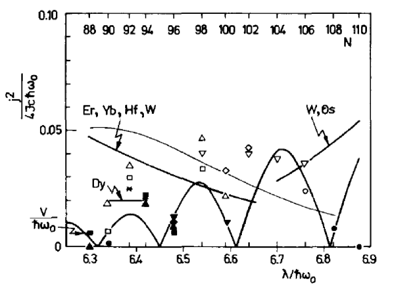
Figure 26: The interaction matrix element $|V|$ between the g- and s-band. The experimental values are shown by the scattered symbols. The theoretical values correspond to the oscillating curve denoted by $V/\hbar\omega_{0}$ with $\hbar\omega_{0}=41A^{-1/3}$ MeV. The experimental values are derived from the experimental function $J_{1}(\omega)$ by an expression given in Ref. [70] that relates $|V|$ to the rapidness of the back bend. The scale of this relation is determined by the quantity $j^{2}/4{\cal J}_{c}$ (cf. Eq. (99), which is shown by the smooth curves (thick lines - experimental, thin lines CSM). Reproduced from [70].

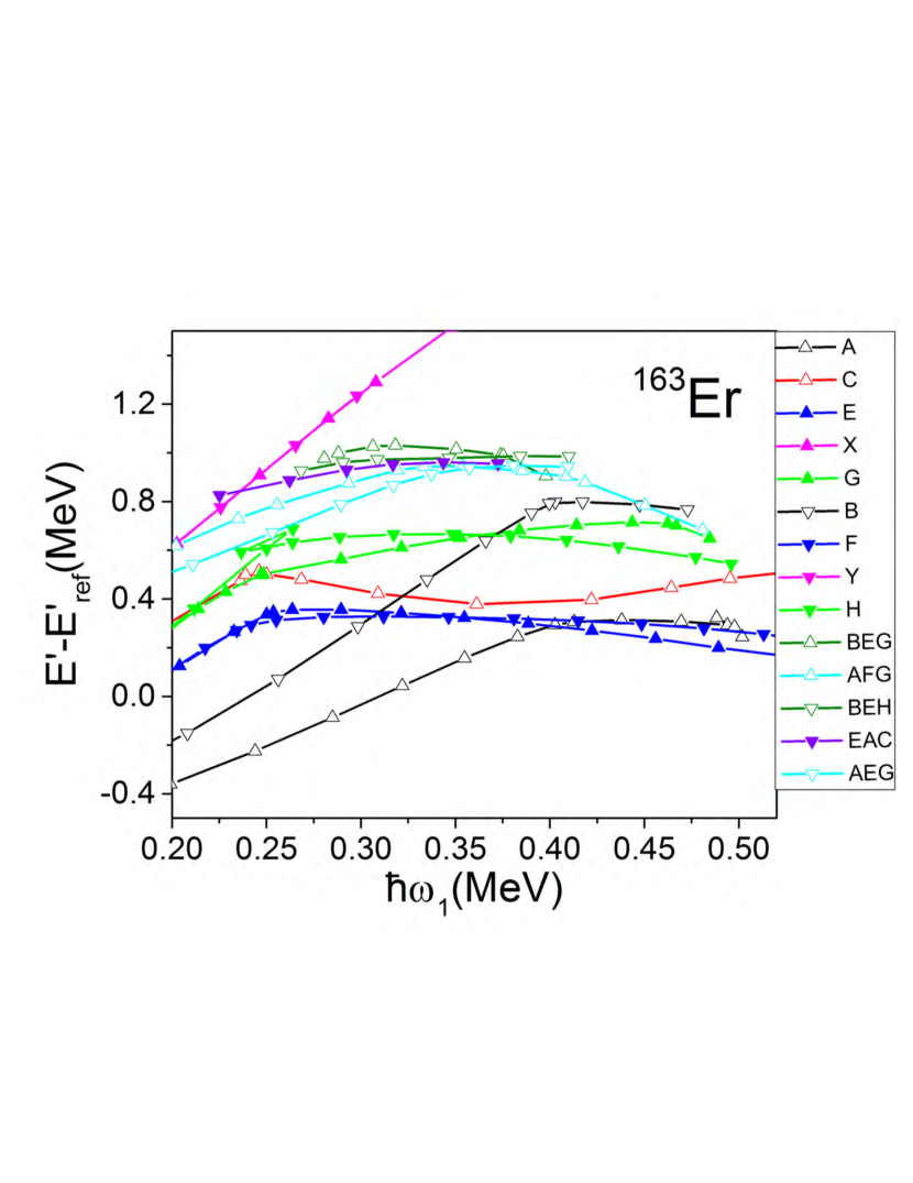
Figure 27: Experimental routhians in ¹⁶³Er relative to the s-band reference routhian $E_{ref}$. The symbol convention is the same as in Fig. 4. Configurations involving two-quasiproton configurations are left away for clarity. The routhians are calculated by means of Eqs. (89,90), where $K=3/2$ is used for g, H; $K=5/2$ for A, B, E, F; $K=9/2$ for BEG, AFG, EAC, AEG; $K=11/2$ for X, Y (cf. [32]). Data from Refs. [32, 25], from which the band labels are adopted.

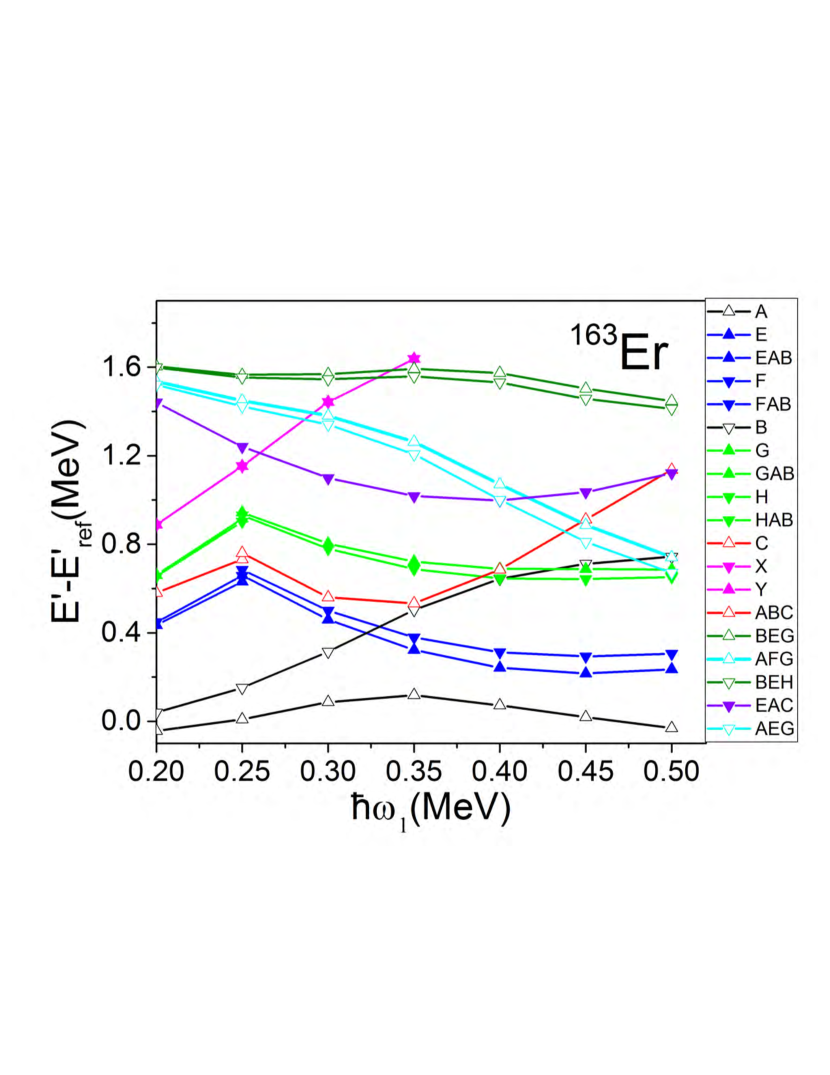
Figure 28: Calculated routhians in ¹⁶³Er relative to the calculated g-band reference routhian $E_{ref}$. Symbol convention as in Fig. 4. Configurations involving quasiprotons and several three-quasineutron configurations are left away for clarity.

The AB-crossing appears in yrast lines of the even-$N$ nuclei ^162,164Er. In Figs. 22 and 23, it is seen at the same frequency as the sudden increase of the negative slope of the bands E, F, G, H in ¹⁶³Er. These quasineutrons are just spectators of the reaction of A and B to the inertial forces. According to this interpretation the [AB] content after the band crossing is explicitly indicated in Fig, 23. The configuration [A] is not disturbed by the AB-crossing. It is “blocked” because both A and B⁺ are occupied. The same holds for [B].

For the systematic analysis of the band crossings it is useful to construct ”diabatic” trajectories . These are the thin lines in Fig. 17 obtained by ”switching off” the interaction, which causes the repulsion between A and B⁺ near the crossing. In this way problems near the crossing are avoided. The rotating mean field becomes a poor approximation there because the basic presumption that the dispersion in angular momentum depends weakly on $\omega$ is violated [74]. This point will be further discussed in section 4.4.

Diabatic tracing is the simplest way to construct diabatic routhians. The quasiparticle routhian (42) is diagonalized for a discrete set of $\omega_{n}$ values. The overlaps between the quasiparticle amplitudes of two adjacent steps, which are given by $[\alpha_{i}^{\dagger}(\omega_{n-1}),\alpha_{j}(\omega_{n})]$, are calculated. The quasiparticle $j$ at $\omega_{n}$ that has the maximal overlap with quasiparticle $i$ at $\omega_{n-1}$ continues the diabatic trajectory. The method depends on the step size. A step of $\Delta\hbar\omega$=0.05 MeV has proven a good choice for medium and heavy nuclei. The tracing sometimes fails when a grid point falls close to the center of a quasicrossing. Usually such problems are easily mended by slightly changing the step size.

Of course, the quasiparticle trajectories found by tracing are still perturbed by the level repulsion near the quasicrossing. Bengtsson an Frauendorf [70] introduced an interaction removal procedure. The routhians in the $\omega$ interval where the level repulsion is substantial are replaced by a low-order interpolation adjusted to the branches above and below the quasicrossing. The deviation of the calculated routhians from the interpolation provides an estimate of the interaction strength that causes the level repulsion. They also suggested an analog analysis of experimental data in terms of two crossing bands, which provided an estimate of the interaction strength that mixes the crossing bands. The two estimates are related in a semiquantitative way. The observed degree of band mixing correlates closely with the mixing degree of the quasiparticle configurations. A striking example of this correlation are the oscillations of the AB-crossing interaction strength shown in Fig. 26. Nikam et al. [75] suggested that these oscillations are a nuclear manifestation of Berry’s Phase encountered in quantum chemistry and solid state physics.

3.6.3 Cranked Shell Model classification of bands

The Cranked Shell Model provides indispensable guidance of which quasiparticle configurations are expected in the yrast region to be associated with the observed multitude of rotational bands. As an example, Fig. 27 shows the routhians in the yrast region of ¹⁶³Er at high spin, which are associated with the Cranked Shell Model quasineutron configurations in Fig. 28. For the high spin region it is more appropriate to use the [AB] configuration, which is yrast in the $N=96$ system, as a reference. It is well approximated by the Harris expression (98) with $i_{r}=3.4\hbar,~{}\Theta_{0}=55.8~{}\hbar^{2}$MeV${}^{-1},~{}\Theta_{1}=0$. The experimental routhians clearly correlate with the Cranked Shell Model pattern. Of course, accurate agreement cannot be expected because the Cranked Shell Model assumes independent quasiparticles and a configuration-independent rotating mean field. Like the time-honored work horses of the spherical Shell Model and the Nilsson Model for deformed nuclei, which are based on the same simplifications, it represents the starting point for a more sophisticated analysis.

A specific feature of the Cranked Shell Model is the appearance of characteristic frequencies of band crossings, which belong to one and the same crossing between two quasiparticle trajectories. It is expected to be seen as a rapid increase of $J_{1}(\omega)$ in all configurations with one of the trajectories occupied and the other free. The crossing shows up as a kink or down bend in the routhian. If both trajectories are occupied or free, no irregularity appears, the crossing is said to be ”blocked”. There are three pronounced crossings seen in Fig. 17, which occur between the high-j i_13/2 quasineutron orbitals: the AB-crossing between A^† and B at $\hbar\omega=$0.25 MeV, the BC-crossing between B^† and C at $\hbar\omega=$0.34 MeV, and the AD-crossing between A^† and D at at $\hbar\omega=$0.38 MeV. The AB-crossing is active in the configurations [E], [F], [G], [H], [C] and seen in Fig. 27 as kinks in the respective bands. It is blocked in the configurations [A] and [B], which are regular around $\hbar\omega=$0.25 MeV. The AD-crossing is active in [B]. It appears as the gradual down bend of the routhian B in Fig. 28 and the kink of B in Fig. 27 at $\hbar\omega=$0.38 MeV, where [B] changes to [ABD]. The BC-crossing is active in [A]. It appears as the gradual down bend of the routhian A and the gradual up bend of ABC in Fig. 28 around $\hbar\omega=$0.34 MeV, where the two configurations interchange character: [A] $\rightarrow$ [ABC] and [ABC]$\rightarrow$ [A]. The interchange corresponds to the crossing of the bands A and ABC seen in Fig. 27 at $\hbar\omega=$0.39 MeV. The BC and AD crossings show analog oscillations as AB as function of the location of the chemical potential $\lambda$ within the i_13/2 shell (cf. Ref. [67]). Therefore, the smoothness of the crossings is sensitive to details of the rotating mean field and may not be accurately accounted for by the Cranked Shell Model, as it is the case in our example.

The Cranked Shell Model approximation implies additivity. That is, the relative routhian $E^{\prime}(\omega)-E^{\prime}_{ref}(\omega)$ of a complex configuration is just the sum the routhians of the constituent quasiparticles. The same holds for the relative angular momentum $J_{1}(\omega)-J_{1ref}$, which is often called the aligned angular momentum or simply the alignment. Plots of the latter have turned out to be a very useful classification tool. Following familiar Shell Model practice, the quasiparticle alignments can be directly derived from experiment. Then they are added up to the total alignment of a multi-quasiparticle configuration. Fig. 29 shows an example of such ”alignment plot”. The gain in alignment by the AB crossing is clearly seen as the group of up-bends clustering around $\hbar\omega_{1}=$0.25 MeV. Summing the experimental quasineutron alignments somewhat overestimates the experimental alignments. The discrepancy can be traced back to a reduction of the pair field $\Delta_{n}$. Using a Cranked Shell Model quasiparticle diagram like Fig. 17 for guidance and combining the information from the alignment plot with the signature and parity quantum numbers (determined by the combining the respective quantum numbers of the constituent quasiparticles), usually allows one to identify the quasiparticle configurations of the lowest bands. The analysis of ¹⁶³Er in Ref.[32] is a good example.

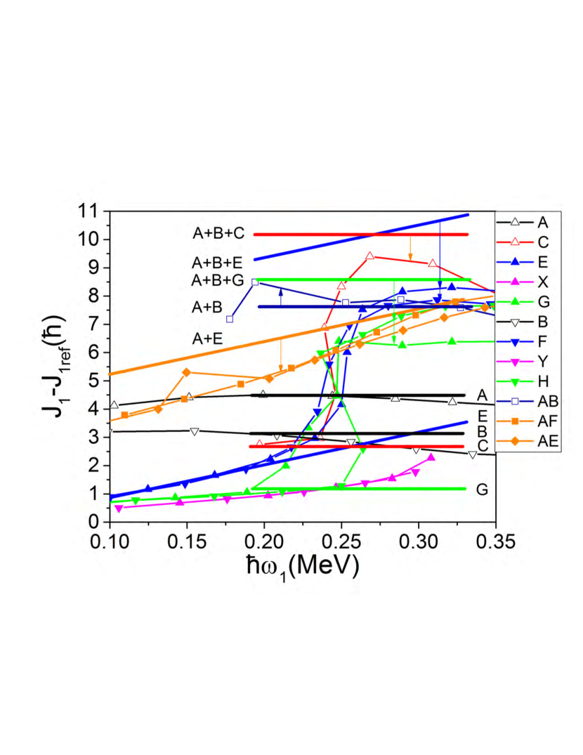
Figure 29: Experimental angular momentum projection on the 1-axis for ^163,164Er relative to the g-band reference $J_{1ref}$. Thin lines with symbols display the data from Data from [32, 25], where symbol convention is as in Fig. 4. The thick lines show some average of the aligned angular momentum in case of one-quasineutron configurations and their sums in case of the multi-quasineutron configurations . The arrows associate the sums with the respective data. Only quasineutron configurations are shown for clarity.

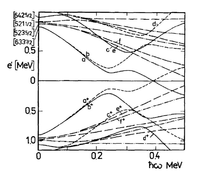
Figure 30: Quasineutron routhian trajectories for $N=98$. The figure shows the trajectories as obtained by diagonalizing the quasiparticle routhian (42) , labeled with lowercase letters, where $+$ indicates the conjugate quasiparticle. Note, the frequency $\omega$ is the frequency $\omega_{1}$ discussed in the text. The figure is constructed using the parameters $\beta=0.267,~{}\Delta=0.79$ MeV. The line types indicate parity and signature $(\pi,\alpha)$: full $(+,+1/2)$, short-dashed $(+,-1/2)$, dot-dashed $(-,1/2)$, long-dashed $(-,-1/2)$. Reproduced from [71], from which the band labels are adopted.

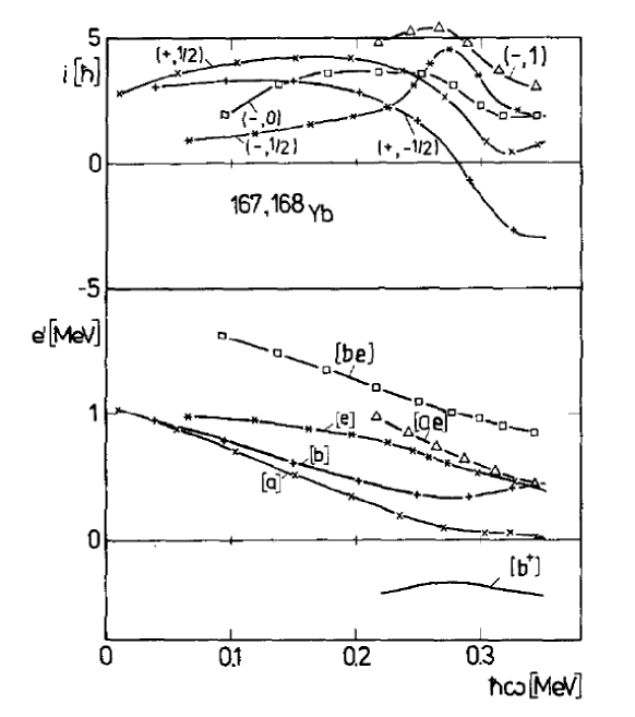
Figure 31: The relative angular momenta $i(\omega_{1})$ and routhians $e^{\prime}(\omega_{1})$ of the experimental rotational bands in ${}^{167}_{70}$Yb₉₇ and ${}^{168}_{70}$Yb₉₈ calculated using the experimental yrast band of ¹⁶⁸Yb as reference. In the upper panel the bands are labeled by parity and signature $(\pi,\alpha)$ in the lower panel by the letters used in Fig. 30. The same symbols are used for the bands in both panels. The conjugate routhian b⁺ is added as $-e^{\prime}_{b}(\omega_{1})$. The figure is constructed adding the experimental even-odd mass difference $\Delta_{eo}$ to all rotational energies of ¹⁶⁷Yb. Note, the frequency $\omega$ is the frequency $\omega_{1}$ discussed in the text. From Ref. [71].

The quasicrossings between high-j routhians are not always as narrow as between a⁺ and b⁺ in Fig. 17. Examples are the neutron numbers with a large value of $V$ in Fig. 26, which indicates a smooth up bend of the quasiparticle routhian a instead of a quasikink. Fig. 30 shows the quasineutron routhians of ${}^{178}_{70}$Yb₉₈. For such cases it may be more appropriate to refer to the original quasiparticle routhians instead of the diabetic ones constructed from them. The (perturbed) yrast band in the $N=98$ system is assigned to the configuration [0] (all $e^{\prime}_{i}(\omega_{1})<0$ occupied), and [a] is the lowest $(+,1/2)$ band in the $N=97$ neighbor. The difference between their total routhians, which is equal to the quasiparticle routhian $e^{\prime}_{a}(\omega_{1})$, can be directly compared with the difference between the experimental total routhian of the $(+,1/2)$ band in the $N=97$ nucleus and the total routhian of the yrast band of the $N=98$ neighbor. The same holds for the other one-quasineutron configurations. The lower panel of Fig. 31 displays the routhian differences between ${}^{177}_{70}$Yb₉₇ and ${}^{178}_{70}$Yb₉₈, which very much look like the quasineutron diagram Fig. 30. The upper panel shows the differences between the pertinent angular momenta $i(\omega_{1})$, which are to be compared with the negative derivatives of the quasineutron routhians in Fig. 30. Of course, the up bend of $e^{\prime}_{a}(\omega_{1})$ in the lower panel of Fig. 31 is caused by the down bend of the total routhian of [0] yrast band in the the $N=98$ system while the total routhian of the configuration [a] in the the $N=97$ system continues smoothly. This blocking feature is more transparently exposed when referring to the diabatic routhian trajectories and a Harris reference. The angular momentum difference for $(-,1/2)$ band [e] shows a bump at $\hbar\omega_{1}=0.28$ MeV, which is absent in the calculated slope of e. The reason is that the presence of the quasiparticle e reduces the neutron pair correlations, which shifts the down bends of quasineutron routhians a⁺ and b⁺ to lower frequency than in the [0] configuration. As a consequence, such they do not completely cancel in the difference, as it is the case for the Cranked Shell Model assuming the same pair gap $\Delta$ for all configurations. Using diabetic routhians, the reduction of the pair correlations caused by the presence of the quasiparticle e shows up as a lowering of the [AB] configuration. The interpretation of the rotational spectra in terms of the Cranked Shell Model quasiparticle configurations without invoking the diabetic trajectories is advantageous when the pair correlations are weak. The studies of nuclei around $N=108$ in Refs. [76, 77] are examples for this kind of analysis.

3.7 Cranked shell correction approach

The selfconsistent cranking model based on the pairing+quadrupole-quadrupole model Hamltonian presented in section 3.1 has limitations when applied to realistic nuclei. The equilibrium shape turns out to be very sensitive to the coupling constant $\chi$, such that local adjustments in various mass regions are necessary for reproducing the experimental information on the nuclear shape. Large changes of deformation within one nucleus, like the appearance of superdeformation at high spin, are also problematic because the pairing+quadrupole-quadrupole interaction does not conserve volume. The cranked shell correction method is a very efficient method to generate a map of the total routhian $E^{\prime}(\beta,\gamma,\omega)$ or the total energy $E(\beta,\gamma,J)$, the minima of which represent the different equilibrium shapes of the rotating nucleus.

Neergard et al. [78] and Andersson et al. [79] generalized the shell correction method to the rotating mean field. The shell correction is calculated from the single particle routhians and it is added to the routhian of the rotating liquid drop, that is Eq. (32) is replaced by

$$E^{\prime}_{SC}(\omega_{1})=\sum\limits_{i\leq N}e^{\prime}_{i}(\omega_{1})-\sum\limits_{i\leq N}\tilde{e}^{\prime}_{i}(\omega_{1})$$ (100)

and Eq.(30) by

$$E^{\prime}(def,\omega_{1})=E_{LD}(def)-\frac{\omega_{1}^{2}}{2}{\cal J}_{rig}(def)+E^{\prime}_{SC}(def,\omega_{1}),$$ (101)

where ${\cal J}_{rig}(def)$ is the classical moment of inertia of rigid rotation [78] . The shape of the rotating nucleus is found by minimizing the total routhian $E^{\prime}(def,\omega_{1})$ with respect to the deformation parameters at a given value $\omega_{1}$. The prediction of the existence of superdeformed nuclei at high spin in these papers, which were found a decade later [80] was a tremendous success of the theory. As an example, Fig. 32 left shows the prediction of superdeformed bands in ¹⁵⁰Gd in Ref. [78], which were identified by Fallon et al. [81]. In their contribution to this Focus Issue, M. A. Riley, J. Simpson and E. S. Paul discuss the phenomenon of super deformation and the history of its discovery in more detail.

The ”total routhian surface” (TRS) represents $E^{\prime}(\beta,\gamma,\omega)$ of the lowest configuration for a given combination of parity and signature $(\pi,\alpha)$ calculated by means of the cranked shell correction method. It is useful for a global survey of the shapes expected near the yrast line. TRS calculations have become quite popular for the interpretation of high-spin data. They are easily accessible as a public domain computer code [82], which is based on the Woods-Saxon potential and includes pairing in a parametrized form. As an example, Fig. 32 right shows the TRS for the configuration [$\pi$h${}_{11/2},~{}\nu$h_11/2] in ¹³⁴Pr.

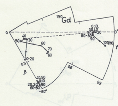
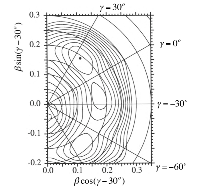
Figure 32: Left: Minima of the total routhian surface for ¹⁵⁰Gd calculated by means of the cranked shell correction approach based on the Nilsson potential without pairing. Reproduced from [78]. Right: Total routhian surface for ¹³⁴Pr calculated by means of the TRS code [82] based on the Woods-Saxon potential including pairing. The configuration is one h_11/2 quasiproton and one h_11/2 quasineutron. The rotational frequency is $\hbar\omega$=0.35 MeV. The contour lines are spaced by 0.2 MeV.

Calculating both $E^{\prime}(\beta,\gamma,\omega)$ and $J(\beta,\gamma,\omega)$, the energy $E(\beta,\gamma,J)$ can be generated by interpolation. Extended collections of such total energy surfaces based on the Woods-Saxon potential and parametrized pairing have been published in Ref. [83]. For more detailed structure analysis one constructs diabatic quasiparticle configurations by various interpolation schemes, which will not be detailed here. A popular method of this type is the Cranked Nilsson-Strutinsky (CNS) approach reviewed by Afanasjev et al. [84], It represents an efficient tool for exploring the high-spin structure of nuclei, because it does not include pair correlations. A public domain computer code, the Ultimate Cranker, is based on the same techniques but includes pairing. It is available online [85]. In their contribution to this Focus Issue, P. M. Walker and F. R. Xu [57] present a further approach along these lines. The shell correction approach applied to a Woods-Saxon potential is combined with a particle number concerving treatment of the pair correlations, which allows them to study the quenching of pairing and the development of the nuclear shape subsequent excitation of quasiparticles. They advanced the approach by taking projection onto good angular momentum into account, which removes problems of the rotating mean field approximation at band crossings (section 3.6.2) and the transition between different symmetries (section 3.8.5).

It has to be stressed here that in addition to the discussed cranked shell correction method the various versions of the self consistent cranking model which are based on energy density functionals have been very successfully applied to study the structure of rapidly rotating nuclei. This area beyond the Unified Model will not be covered in my contribution, which focuses on the aspects of symmetries and coherence of the rotating mean field. The contributions to this Focus Issue by L. Egido [41] and P. G. Reinhard [39] and the review articles by M. Bender et al. [38] and D. Vretenar et al. [86] are good starting points for exploring these developments.

3.8 Rotation about a tilted axis

3.8.1 The spinning clockwork picture

Stable uniform rotation appears for the axis with the largest moment of inertia. As discussed in Sect. 2, the Unified Model assumes that the nucleus rotates like an irrotational quantum liquid, which implies the following. Rotation about a symmetry axis is impossible. The shape dependence of the moments of inertia is given by Eq. (8), which assigns the largest moment of inertia to the medium axis of the triaxial nucleus. It needs to be emphasized that this is in contrast to a rigid ellipsoidal body, for which the maximal moment of inertia belongs to the short axis. The irrotational-liquid behavior emerges because the nucleus is composed of two kinds of indistinguishable fermions. Accordingly, the ground state band of an even-even triaxial nucleus corresponds to rotation about the medium axis with the maximal moment of inertia, which becomes the one of the axis perpendicular to the symmetry axis in the special case of axial symmetry.

This traditional view misses essential aspects of nuclear rotation which the study of the rotating mean field has revealed. Unlike the particles in a macroscopic liquid the nucleons have a mean free path that is larger than the size of the nucleus. As a consequence their motion is restricted by quantization. The quantization of the angular momentum of the nucleonic orbits determines the way nuclei rotate. In order to illustrate the essential consequences it is useful viewing the nucleus as a clockwork of small gyroscopes, which carry a fixed angular momentum. The essence of the analogy is the approximately constant angular momentum of the high-j nucleonic orbitals, which is fixed by quantization. The gyroscopes represent the nucleonic orbitals, which are coupled to the deformed potential by their non-isotropic density distribution. The left panel of Fig. 21 depicts a gyroscope representing a high-j orbital. (The density distribution of low-j orbitals is less torodial but still deformed, except s-orbitals.) As discussed in section 3.5 and in more detail in the A, the orientation of the gyroscopes with respect to the density distribution results from the balance between the inertial forces and the torque exerted by the deformed potential. The resulting arrangement in the clockwork generates nucleon density distribution which generates the average field in a selfconsistent way. The interplay is governed by the principle that the short-range attractive interaction favors large overlap of the densities of the orbitals and the Pauli Principle.

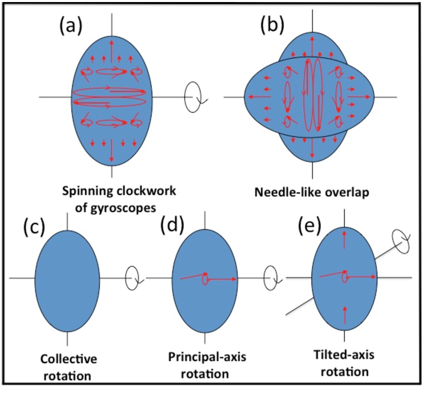
Figure 33: The nuclear clockwork of gyroscopes. The figure shows in a schematic way the orbits of the angular momentum vectors of the occupied orbitals. The vectors are distributed over the volume for graphical reasons. They should be thought originating from the center. The lower row shows only the rearrangement compared to (a), that is (c) is simplified (a).

Fig. 33 (a) illustrates the arrangement of the gyroscopes for the ground state of an even-even axial nucleus. The figure depicts the precessional cones of the angular momentum vectors of the gyroscopes. The orbitals arrange back-to-back, which gives good overlap between their density distributions and is also favored by the pair correlations. For a partially filled shell this results in a prolate density distribution and a prolate potential. (For the ground state of a triaxial nucleus the arrangement of the gyroscopes consists of one set of back-to-back orbital pairs aligned with the long axis and and another set of pairs aligned with the short axis, which generates a triaxial potential (see A)).

Turning the clockwork around the symmetry axis does not change the system. Fig. 33 (b) shows that turning the clockwork around the short axis makes a large difference which mainly comes from the reorientation of the many angular momentum vectors. The displacement of the surface bump of the density distribution is much less important, keeping in mind that the axis ratio is largely exaggerated in the figure. This observation is at variance with the Unified Model, which considers the deformation of the nuclear surface as the origin of the rotational degrees of freedom. In fact, the overlap of the product of the quantal wave functions of the orbitals in Fig. 33 (b) falls off rapidly with the rotation angle (see section 4.4). As a consequence, one may generate a collective wave functions with a large number of nodes by superposing the different orientation of the needles, which means an extended rotational band.

The angular momentum of the ground band is generated by gradually aligning the gyroscopes with the rotational axis. The needed energy determines the moment of inertia. Section 4.4 will discuss the emergence of the rotational degree of freedom in a more quantitative way. Generating the angular momentum of a rotational band by gradually aligning two long vectors composed of nucleonic angular momenta was first discussed by Danos and Gillet [93]. Fig. 33 (a) illustrates their ”stretch” scheme. One of the two vectors is thought to be constructed by stretched coupling of the valence nucleons shown in the upper half and the other vector by stretched coupling the valence nucleons shown in the lower half. In the ground state the two vectors have opposite direction. They gradually align along the band increasing the angular momentum. The capability of the stretch scheme to account for the energetics of realistic rotational bands was never demonstrated for the ground state bands of even-even nuclei, for which it was conceived. However in a modified version, it very well describes Magnetic Rotation, which will be discussed in section 4.2.

From Fig. 33 (b) it is clear that a rotation by 180^∘ about the short axis brings the clockwork back to its original state, which implies that the ground band contain only even spins. As a consequence the ground state band contains only even $I$.

If the rotational motion is slow enough, the alignment of the individual orbitals with the rotational axis is small and proportional to the rotational frequency $\omega$, and the total angular momentum is proportional to $\omega$ as well. The rotational motion is characterized by three principal moments of inertia ${\cal J}_{\mu}$ and the well known linear relation between the angular momentum $\vec{R}$ and the angular velocity $\vec{\omega}$,

$$R_{\mu}={\cal J}_{\mu}\omega_{\mu}.$$ (102)

Only uniform rotation about principal axes is possible.

The rotational response of clockwork (a) is the one of the collective rotor of the Unified Model. To simplify the following discussion In the lower row of Fig. 33 the many orbitals that generate the collective angular momentum are left away in order to simplify the discussion, i. e. (c) represents (a). Part (d) illustrates case when one or more quasiparticles align with the short axis, which is the rotational axis. Turning the arrangement of the gyroscopes by 180^∘ about the principal short axis leaves it invariant. Therefore the signature remains a good quantum number that labels the $\Delta I=2$ rotational band. More generally, one of the principal axes of a triaxial nucleus remains the rotational axis when one or more quasiparticles align with it. The arrangement appears as a $\Delta I=2$ band corresponding to the signature of the arrangement.

3.8.2 Appearance of tilted rotation

Fig. 33 (e) illustrates a case when the gyroscopes are asymmetrically oriented, such that their angular momenta add up to a finite component $J_{3}$ and along the symmetry axis and a perpendicular component $i_{1}$, which with the angular momentum of remaining nucleons ${\cal J}_{1}\omega_{1}$ adds to $J_{1}=i_{1}+{\cal J}_{1}\omega_{1}$. The axis of uniform rotation will be tilted away from the principal axes. Uniform rotation appears when the rotational axis $\vec{\omega}$ has the direction of total angular momentum $\vec{J}$, which requires that $\tan\vartheta=J_{3}/\left(i_{1}+{\cal J}_{1}\omega\sin\vartheta\right)$. This condition can be met by the appropriate value of $\vartheta$.

The example demonstrates that a nucleus may uniformly rotate about an axis that differs from one of the principal axes of its mass density distribution. The tilted rotation of nuclei is due to the quantized angular momentum of the nucleonic orbitals, which carry a fixed amount of angular momentum large enough to tilt the rotational axis. Such a mode does not appear for a classical rotating rigid body, which obeys the relations (102) well known from textbooks on mechanics. The reason is that its constituents do not carry angular momentum of their own, because they are considered as point masse, not as gyroscopes. A rotating drop of ideal liquid obeys Eqs. (102) as well if the flow is irrotational (see Ref. [6] section 6A-5). However, a classical liquid may also uniformly rotate about an axis different from the principal axes of its density distribution. This possibility was already pointed out by Riemann [94] for an ellipsoidal self-gravitating fluid. The origin of the tilt of the rotational axis are deviations from irrotational flow which generate vorticity. Thus, the tilt of the rotational axis is due to an intrinsic vorticity of the system. This applies to nuclei as well, because the high-j orbitals appear as pronounced vortices in the microscopic current pattern of a rotating nucleus (see discussion in Ref. [95]).

3.8.3 Tilted axis cranking solutions of axial nuclei

The angular momentum geometry has to be planar. As discussed in section 3.2.3, planar tilted axis cranking solutions show up as $\Delta I=1$ bands, i.e. the two signatures are degenerate, merged into one sequence. The $E2$ transitions between states with $I$ and $I\pm 1$ are strong, because the charge distribution is asymmetric with respect to the tilted axis of rotation. The stretched $M1$-transitions are enhanced, because the transverse magnetic moments of the different quasiparticles add up. The $B(M1)$ values need not be large in all cases, because the transverse magnetic moments of the contributing quasiparticles can have different signs. For principal axis cranking solutions, both types of transitions connect two configurations of opposite signature, which are non-degenerate in general. The transition can only be of the order of single-particle transitions, because they connect different quasiparticle configurations. Hamamoto and Sagawa [96] studied the electromagnetic transition matrix elements between different Cranked Shell Model configurations.

Let us continue to use ${}^{163}_{66}$Er₉₇ as an illustrative example. Fig. 34 shows the quasiparticle levels as functions of the tilt angle $\vartheta$. Such diagrams permit a first guess of the equilibrium angle by adding the quasiparticle routhians $e^{\prime}_{i}(\omega,\vartheta)$ to the vacuum routhian and looking for the minimum of the sum with respect to $\vartheta$. The vacuum behaves like a collective rotor (see section 3.8.1, Eq. (102). If we consider an axial nucleus, it has only the component $R_{1}\approx\omega{\cal J}\sin\vartheta$ perpendicular to the symmetry axis and its routhian is $E^{\prime}_{0}\approx-(\omega\sin\vartheta)^{2}{\cal J}/2$.

The quasineutron levels E and F emanating from the Nilsson state $[523]5/2^{-}$ are strongly coupled to the deformed potential. They have $j_{3}\approx\pm 5/2$ and $j_{1}\approx 0$. This is reflected by the $\vartheta$ dependence, which is close to $\mp 5/2~{}\omega\cos\vartheta$. Occupying E results in an equilibrium angle $\vartheta<90^{o}$. As expected for a tilted axis cranking solution, the band [E] appears as a $\Delta I=1$ sequence in Fig. 35. Further examples of strong coupling to the deformed potential are quasineutron level $[505]11/2^{-}$ and the quasiproton levels $[404]7/2^{+}$ and $[523]7/2^{-}$, which are all seen as $\Delta I=1$ bands.

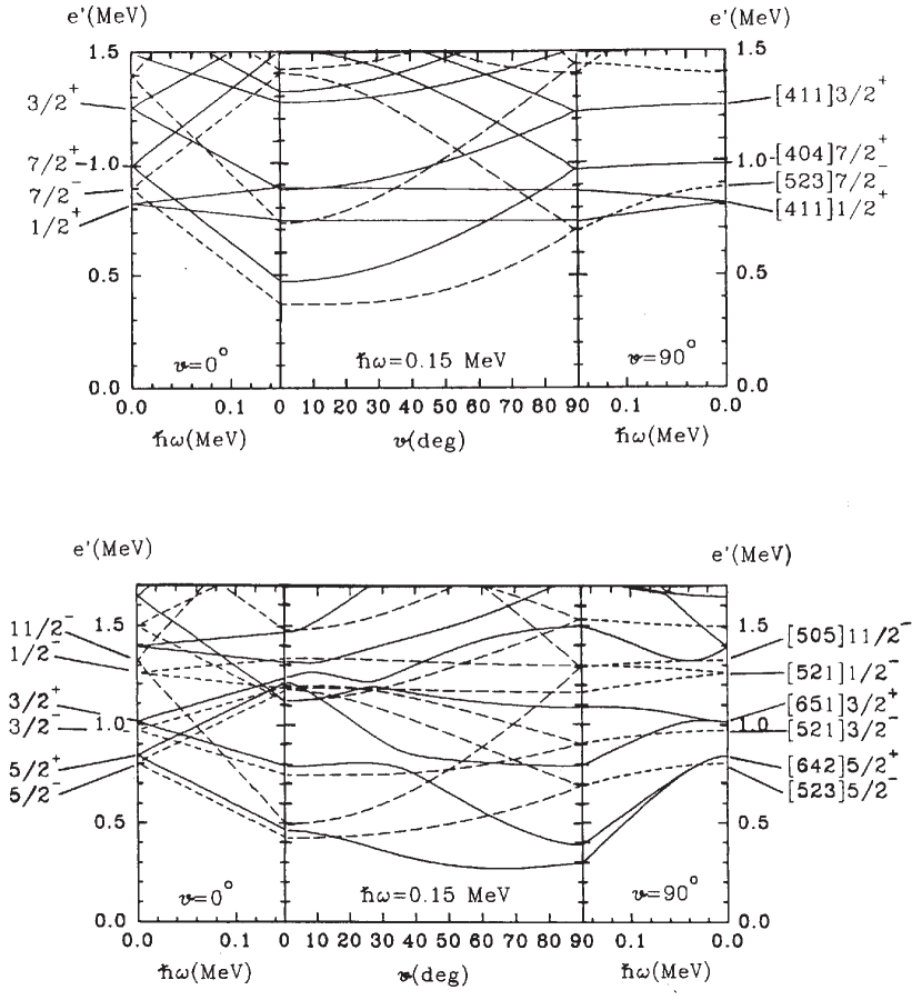
Figure 34: Quasiproton routhians for $Z\approx 66$ (upper panel) and quasineutron routhians for $N\approx 97$ (lower panel) as functions of the tilt angle $\vartheta$ at the frequency $\omega=0.15$ MeV$/\hbar$ (middle parts). The variation with $\omega$ is shown in the left-hand parts for $\vartheta=0^{o}$ and in the right-hand parts for $\vartheta=90^{o}$. Full lines: positive parity. Dashed-dotted lines: negative parity. The parameters are $\varepsilon=0.252,~{}\gamma=0^{o},~{}\varepsilon_{4}=-0.004,\Delta_{p}=0.87~{}\mathrm{MeV},~{}\Delta_{n}=0.80~{}\mathrm{MeV}$. From Ref. [97].

Figure 35: Experimental routhians of the rotational bands in ¹⁶³Er. The bands are labeled by the Nilsson quantum numbers. In Fig. 9, [642] is labeled by A and B and [523] by E and F. The tilted axis cranking routhians are shown as the large symbols on the two vertical lines where the calculations have been carried out. The same symbols are used for the experiment and calculations. A rigid rotor reference routhian $-\omega^{2}\times 31.7\hbar^{2}\mathrm{MeV}^{-1}$ is subtracted. From Ref. [98] after Ref. [97].

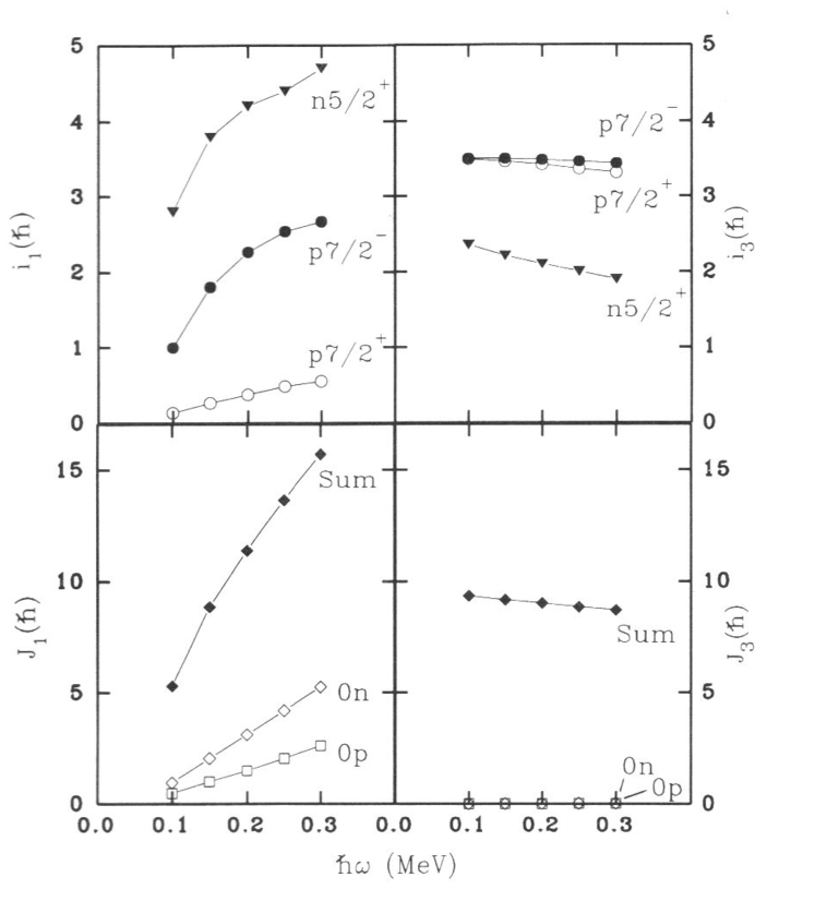
Figure 36: The angular momentum composition of the three-quasiparticle configuration K1 in ¹⁶³Er calculated in the tilted axis cranking approach. The angular momentum expectation values for the short 1-axis and the long 3-axis are displayed. The total angular momentum $J_{1,3}$ is the sum of the quasiparticle vacuum parts denoted by $[p0]$ and $[n0]$ and the quasiparticle contributions $i_{1,3}$, where the short hand notation is used: $p7/2^{+}=\pi[404]7/2^{+},~{}p7/2^{-}=\pi[523]7/2^{-},~{}n5/2^{+}=\nu[642]5/2^{+}$. From Ref. [97].

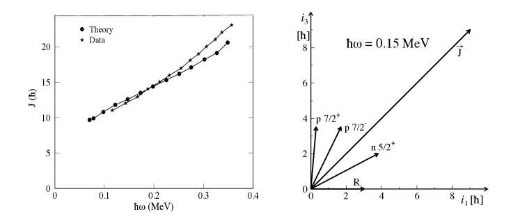
Figure 37: Left panel: Comparison of the total angular momentum calculated by means of tilted axis cranking with experimental values of the three-quasiparticle configuration K1 in ¹⁶³Er. Right panel: Vector diagram of the angular momentum composition at $\omega=0.15~{}\mathrm{MeV}/\hbar$ obtained by the calculations shown in the left panel and Fig. 36. The collective angular momentum of the quasiparticle vacuum is denoted by $R$. Taken from Ref. [97].

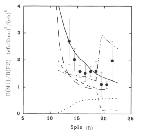
Figure 38: Experimental ratios of $B(M1,I\rightarrow I-1)/B(E2,\rightarrow I-2)$ for the K1 band in ¹⁶³Er. They are compared with the tilted axis cranking calculations (long dash) and the Dönau-Frauendorf vector model Eqs. (105). Different configurations are shown: $[p7/2^{+}p7/2^{-}n5/2^{+}]$ (full), $[n11/2^{-}n3/2^{-}n5/2^{-}]$ (medium dash), $[n11/2^{-}n3/2^{-}n5/2^{+}]$ (dot), $[p7/2^{+}p7/2^{-}n5/2^{-}]$. The short hand notation is the same as in Fig. 34 and $n11/2^{-}=\nu[505]11/2^{-},~{}n3/2^{-}=\nu[521]3/2^{-},~{}n5/2^{-}=\nu[523]5/2^{-}$. The experimental $i_{1}(\omega_{1})$ is derived from the $\alpha=+1/2$ branch of $n5/2^{+}$. The transition matrix element $Q_{t}=7eb$ (defined by footnote to Eq. (82)) is used in the calculation of the $B(E2)$ values. Taken from Ref. [97].

The quasineutron routhians A and B emanating from $[642]5/2^{+}$ show a more complex behavior. The lower routhian A has a very shallow minimum at $\vartheta\approx 60^{o}$. Fig. 72 shows the location of the minimum of the lowest quasiparticle state with respect to $\vartheta$ and $\gamma$ for different shell filling. For $\vartheta=60^{\circ}$ and $\gamma=0^{\circ}$ the shell filling parameter is close to -0.2, which is about the location of the neutron chemical potential $\lambda_{n}$ in the i_13/2 shell. The lowest quasineutron is only weakly coupled to the deformed potential, because its quadrupole moment is strongly reduced by the pair correlations. (It is half particle and half hole.) For this reason, the minimum is shallow. The upper routhian B has its minimum at $\vartheta=90^{o}$, because it changes (through a quasicrossing with C) into the $\Omega=-5/2$ state at $\vartheta=0^{\circ}$. Combined with the vacuum routhian, both configurations [A] and [B] are principal axis cranking solutions with $\vartheta=90^{o}$, which have been discussed in section 3.6.

The pair of parallel trajectories emanating from the Nilsson state $[521]1/2^{-}$ is an example for a pseudospin doublet. Their routhians do not change with $\vartheta$ and their distance equals $\hbar\omega$. They behave in this way, because their angular momentum is approximately equal to the pseudo spin, which is decoupled from the deformed field. It takes the direction of $\vec{\omega}$ or opposite to it, corresponding to a routhian $e^{\prime}(\vec{\omega})\approx e(\omega=0)\pm\hbar\omega/2$. The concept of pseudo spin and the reason for the decoupling are explained in Ref. [14]. The vacuum routhian keeps $\vec{J}$ parallel to the 1-axis and the solution is of the principal axis cranking type. The levels of the $I+1=-1/2+2n$ sequence have the same energy as the levels with $I=1/2+2n$. The ground state of ¹⁷¹Yb is $[521]1/2^{-}$. The rotational band consist of the expected doublets. The routhians of the quasiproton level $[411]1/2^{+}$ do not change with $\vartheta$ too, because they combine to pseudo spin singlet state. Doublet $\Delta I=2$ sequences that correspond to the signatures $\alpha=\pm 1/2$ of the orbital $[411]1/2^{+}$ are observed in the odd-$Z$ Tb isotopes.

The band K1 in Fig. 9 is assigned to the three-quasiparticle configuration $[\pi 7/2^{+},\pi 7/2^{-},\nu 5/2^{+}]$, where each of the quasiparticles occupies the lower of the two branches emanating at $\vartheta=0^{\circ},90^{\circ}$ and $\omega=0$ in Fig. 34. The composition of the total angular momentum is displayed in Fig. 36 and the right panel of Fig. 37. The tilt angle $\vartheta(\omega)$ grows as a consequence of the increasing collective angular momentum $R$, but remains below $90^{\circ}$. Accordingly, band K1 is observed as a $\Delta I=1$ sequence. The left panel of Fig. 37 compares the experimental function $J(\omega)$ of band K1 with the tilted axis cranking calculation. Fig. 35 includes the routhians calculated by means of tilted axis cranking for two values of the frequency $\omega$. The agreement between theory and experiment is typical for the other tilted axis cranking calculations in well deformed nuclei. Tilted axis cranking calculations account for the transition intra band $M1$ and $E2$ rates as well. As an example, Fig. 38 shows the ratios $B(M1)/B(E2)$ for the K1 band. The calculation well follows the experiment. It is somewhat smaller than the experiment, which can be traced back to general inaccuracies of the mean field $g$-factor values of the involved quasi-particles.

The example ¹⁶³Er is typical for the accuracy of tilted axis cranking calculation in reproducing the experiment. Further phenomena that have been studied in the framework of the tilted axis cranking approach can be found in Ref. [14], as the interplay of high-K and low-K bands in the mass 180 region or the decay of high-K isomers. P. M. Walker and F. R. Xu [57] extensively discuss the high-K isomers in their contribution to this Focus Issue,

3.8.4 Approximate tilted axis cranking solutions - relation to principal axis cranking

In the strong coupling limit, tilted axis cranking approximates the Unified Model semiclassically. The total angular momentum is composed only of the collective part $J_{1}=\hbar R$ and $J_{3}=\hbar K$, which is constant. The energy

$$E=\frac{R^{2}}{2{\cal J}}=\frac{I(I+1)-K^{2}}{2{\cal J}}$$ (103)

is the same as in the Unified Model. The tilt angle is given by

$$\cos\vartheta=\frac{K}{I+1/2}.$$ (104)

For this value of $\vartheta$, the tilted axis cranking expressions (75-69) agree with the transitions probabilities in the Unified Model when the Clebsh-Gordan coefficients are approximated by their high-spin asymptotic values. This approximation is very accurate except near $I=K$.

The Cranked Shell Model uses a less stringent approximation. The assumption $J_{3}=\hbar K$ is kept but $J_{1}$ is calculated by means of principal axis cranking at the frequency is $\omega_{1}=\omega\sin\vartheta$, where $\vartheta$ given by (104). It amounts to neglecting the term $-\omega\hat{J}_{3}\cos\vartheta$ in the mean field routhian. If $J_{3}$ is not too large, the band starts at a relatively low frequency and $\vartheta$ changes rapidly from $0^{o}$ to $90^{o}$. The neglected term is not too important if the coupling of the quasi-particle orbital to the deformed potential is much stronger than $-\omega\hat{J}_{3}\cos\vartheta$. Then it is a good approximation to take only $-\omega\hat{J}_{1}\sin\vartheta$ into account. This is not the case for weakly coupled orbitals or small deformation. Of course, the Cranked Shell Model approximation becomes better and better when $\vartheta$ approaches $90^{o}$.

Dönau and Frauendorf [99, 100] worked out the transition probabilities for the Cranked Shell Model approximation. They are given by Eqs. (69) - (77) using the strong coupling limit (104) for the tilt angle $\vartheta$.. The intrinsic components of the magnetic moments of the excited quasi-particles $i$ are calculated by means of the relations

$$\mu_{\nu}=\sum\limits_{i}g_{i}j_{\nu,i},~{}~{}\mu^{c}_{\nu}=g_{R}(J_{\nu}-\sum\limits_{i}j_{\nu,i}),~{}~{}\nu=1,~{}3,$$ (105)

where $\mu^{c}_{1}$ denotes the collective magnetic moment of the quasiparticle vacuum. The global estimate $g_{R}\approx Z/A$ is usually good enough. The gyromagnetic ratios $g_{i}$ are either taken from the experiment or calculated from the mean field solutions at $\omega_{1}=0$. The components $j_{3,i}$ are set equal to the angular momentum projection $\hbar\Omega_{i}$ at $\omega_{1}=0$. The components $j_{1,i}$ are either calculated as $\langle j_{1}\rangle$ by means of the Cranked Shell Model or extracted as the aligned angular momenta $i_{i}$ from the differences between the experimental functions $J_{1}(\omega_{1})$ with and without the quasi-particle $i$ present. This calculation scheme for transition probabilities is referred to as the ”semiclassical vector model” or ”Dönau-Frauendorf model”. The possibility of extracting the aligned angular momenta and the g-factors from experiment substantially improves the accuracy of the calculation.

Fig. 36 shows that $j_{i,3}=\hbar\Omega_{i}$ is a good approximation for the well deformed nucleus ¹⁶³Er. Fig. 38 includes calculations of the $B(M1,I\rightarrow I-1)/B(E2,\rightarrow I-2)$ ratios which exploit the flexibility of the vector model. The quasiparticle alignments $i$ are calculated from taking the differences between appropriate quasiparticle configurations in ¹⁶³Er and ¹⁶³Tm. The calculations use experimental gyromagnetic ratios $g_{K,i}$, which are average values derived from $B(M1)$ values of the pertinent one-quasiparticle bands for the rare earth region. Since information of the same kind from related configurations is used, it is not surprising that the agreement with the experiment is better than for the microscopic tilted axis cranking calculation.

The Cranked Shell Model is quite commonly used because of its simplicity. The spectrum of rotational bands can be constructed by occupying the quasiparticle levels in a single quasiparticle diagram like Fig. 17. This allows a quick semi-quantitative classification of the multiple band spectra provided by $\gamma$ spectroscopy. A certain price of this simplicity is the fact that high-K configurations, which gain much energy by the tilt, appear as relatively highly excited quasiparticle configurations in a Cranked Shell Model quasiparticle routhian, whereas they are close to the yrast line and strongly populated in experiment.

The Cranked Shell Model can be seen as an approximation to tilted axis cranking, which generates the best possible mean field solution. The Cranked Shell Model amounts to extrapolating the tilted axis cranking quasiparticle routhians from the values calculated at $\vartheta=90^{o}$ by means of the expression

$$e^{\prime}_{i}(\omega,\vartheta)=e^{\prime}_{i}(\omega,90^{o})-\omega\left(j_{1,i}(\sin\vartheta-1)+\hbar\Omega_{i}\cos\vartheta\right).$$ (106)

Fig. 34 demonstrates that this is a quite decent approximation for a number of quasi-particles. But it does not fully account for the complex behavior of the $i_{13/2}$ quasineutrons as functions of $\vartheta$. Within the approximation (106), the Cranked Shell Model transformation (89) of the experimental energies $E(I)$ to experimental routhians $E^{\prime}(\omega_{1})$ accommodates the energy gain due to tilt. The possible configurations for high-K bands can be singled out of the low-K configurations by the criterion that they must contain signature-degenerate quasiparticle routhians.

In their contribution to this Focus Issue, P. M. Walker and F. R. Xu [57] discuss the phenomenon of high-K isomerism. Their theory combines cranking about the principal 1-axis with the shell-correction method and a particle number conserving treatment of pairing to account for the attenuation of the pair correlations by quasiparticle excitations. As discussed above for the Cranked Shell Model, the angular momentum component along the symmetry axis is approximated by fixing it to $J_{3}=\hbar K$, which is a good approximation for well deformed nuclei and large values of $K$. The fixed-$K$ approximation becomes bad for the weakly deformed nuclei, because the responses to $-\omega j_{1}$ and $-\omega j_{3}$ are comparable. It is also problematic for triaxial nuclei because the principal axis cranking calculations provide only the 1-component of the angular momentum. An estimate of the $J_{3}$ component becomes rough if not impossible.

3.8.5 Change of symmetry

The discussed symmetry types are reflected by the multiplicity of the bands. If the rotational axis coincides with a principal axis one observes a $\Delta I=2$ sequence. If the rotational axis lies in a principal plane one observes a $\Delta I=1$ sequence. If the rotational axis points out of a principal plane one observes two degenerate $\Delta I=1$ sequences. With increasing rotational frequency, the direction of the rotational axis may change from one to another symmetry type, which implies changing the interpretation of the mean field solution. In an infinite system sudden symmetry changes appear as singularities at a phase transition. In a finite system, as the nucleus, the change is gradual. When changing from lower to higher symmetry the band with the higher multiplicity splits into two bands of lower multiplicity, which are associated with different mean field configurations. Vice versa, when changing from higher to lower symmetry two bands of lower multiplicity associated with different mean field configurations merge into one band of higher multiplicity. Both cases are observed. In the following we discuss symmetry changes by analyzing energies and transition probabilities obtained by diagonalizing the quasiparticle triaxial rotor Hamiltonian (37). Since the quasiparticle triaxial rotor model conserves angular momentum, it describes the smooth transition from one to the other symmetry type. In this respect we consider the quasiparticle triaxial rotor model results as ”exact” and compare them with the cranking approximation to the same model case.

For now we consider the case of axial nuclei, we will return to the symmetry changes in section 3.8.6. A typical scenario is that some quasiparticles generate angular momentum along the 3-axis ($\vartheta=0^{\circ}$) and that there is collective angular momentum $\vec{R}$ pointing along the 1-axis ($\vartheta=90^{\circ}$), which results in a tilt angle $0^{\circ}<\vartheta<90^{\circ}$. As $R$ increases along the band the tilt angle $\vartheta$ increases, which for certain quasiparticle configurations may approach 90^∘, where the ${\cal R}_{z}(\pi)$ is restored. Correspondingly, the $\Delta I=1$ sequence changes into two $\Delta I=2$ sequences.

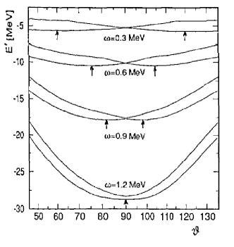
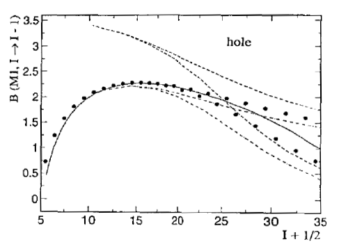
Figure 39: Left panel: Total routhian of an h_11/2 hole coupled to an axial rotor as function of the tilt angle $\vartheta$ for several rotational frequencies $\hbar\omega$ ($\hbar=1$). The arrows indicate the location of the minima. The configuration changes at the kinks in the upper curves. Right panel: Reduced transition probabilities $B(M1,I\rightarrow I-1)$ of an h_11/2 hole coupled to an axial rotor as a function of the spin $I$. The unit is $(g_{qp}-g_{R})\mu^{2}_{N}$. The dots are the results of the exact results obtained by diagonalizing the hole-rotor model. The full drawn curve shows the tilted axis cranking values. The lower pair of dashed curves show the values obtained by means of the Dönau-Frauendorf vector model Eqs. (105). The upper pair of dashed curves shows the values obtained by means of Eq. (3.8.5). From Ref. [101].

Frauendorf and Meng [101] investigated the transition region in the framework of the quasiparticle triaxial rotor model presented in section 2.7. For comparison the total cranking routhian is constructed for the model,

$$E^{\prime}(\omega,\vartheta)=e^{\prime}(\omega,\vartheta)-\omega^{2}\sin^{2}\vartheta\frac{{\cal J}_{1}}{2}.$$ (107)

The quasiparticle routhian $e^{\prime}(\omega,\vartheta)$ is eigenvalue of the cranking Hamilonian (62) restricted to an h_11/2 subshell. The rotor moment of inertia ${\cal J}_{1}$ describes the routhian of all other nucleons. It is set equal to the moments of inertia ${\cal J}_{1}={\cal J}_{2}$ used in the quasiparticle triaxial rotor (37) (${\cal J}_{3}=0$). The deformation $\beta=0.3$ chosen. From the examples studied in Ref. [101], we discuss the case of a pure h_11/2 hole coupled to the axial rotor. The left panel of Fig. 39 shows the total routhian (107) as a function of the tilt angle $\vartheta$. The high-j hole prefers $\vartheta=0$ because its angular momentum aligns with the 3-axis. The collective term prefers $\vartheta=90^{\circ}$. The equilibrium angle lies at the minimum of the total rothian, where the two tendencies are balanced. With increasing $\omega$ the minimum moves toward $\vartheta=90^{\circ}$, which it reaches for $\hbar\omega\approx 1$MeV. Below this frequency the minimum $\vartheta<90^{\circ}$ is associated with the two degenerate signatures of the $\Delta I=1$ band. Above, e. g. at $\hbar\omega=1.2$ MeV, the lower of the two minima represents the $\Delta I=2$ band with $\alpha=-1/2$ and the upper minimum the $\Delta I=2$ signature partner band $\alpha=1/2$.

In order to avoid over counting the number of configurations that represent rotational bands, it is helpful to refer to a symmetric graph like the left panel of Fig. 39. Below $\hbar\omega=1$MeV there are always two degenerate minima symmetric to 90^∘, which is the manifestation of breaking the ${\cal R}_{1}(\pi)$ symmetry. These two minima generate the $\Delta I=1$ band by combining their pertinent configurations to even and odd superpositions, which are the two signatures comprising the band. As seen in the figure, the two configurations represent the continuation of the configurations with the hole on the higher level (inside the kink), which are already taken into account. Therefore they must be discarded as configurations assigned to bands. For other one-quasiparticle configurations the spurious ones can be eliminated by the same reasoning. Elimination becomes more involved for a larger number of excited quasiparticles, where rules are formulated in Refs. [88] and [101].

The tilted axis cranking solution very accurately approximates the energy of the exact hole-rotor solution up to $\hbar\omega=0.7$ MeV, where the two signatures begin to separate. For $\hbar\omega>1.2$ MeV the two principal axis cranking solutions at $\vartheta=90^{\circ}$ very well reproduce the energy of the two $\Delta I=2$ bands, in particular the small signature splitting. In the transition region the tilted axis cranking energy lies half-way between the energies of the two signatures branches.

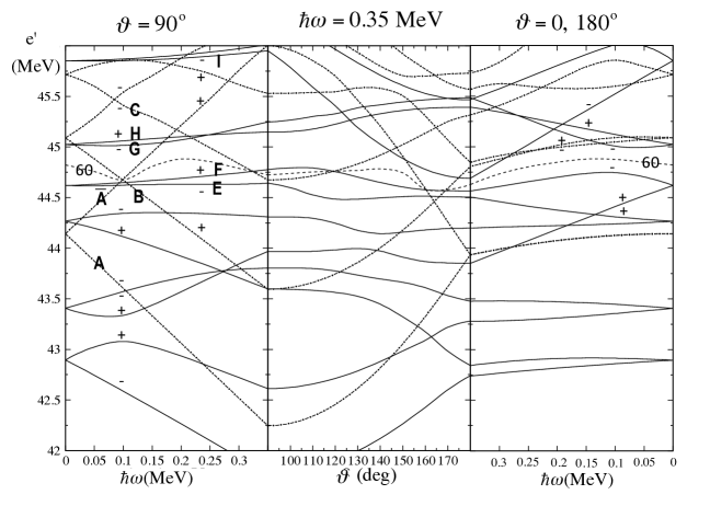
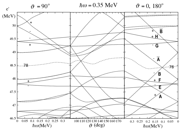
Figure 40: Single-particle routhians (protons uper panel , neutrons lower panel) around the Fermi surface of ¹³⁸Nd calculated for the deformation parameters $\varepsilon_{2}=0.17$, $\gamma=30^{\circ}$. Full line $\pi$=+, dash-dot line $\pi=-$. In case of rotation about the long axis, $\vartheta=0$, and about the short axis, $\vartheta=90^{\circ}$, the signatures $\alpha=\pm 1/2$ are indicated by $\pm$, respectively. The middle panel connects the two axis at the indicated frequency. The angle in the middle part is either $\vartheta$ or $180^{\circ}-\vartheta$, because the pertinent rotations are related by inverting the orientation of the l-axis, which leaves the potential invariant. The h_11/2 orbitals are labelled by A, B, C and the $\pi=+$ orbitals by E, F, … . Taken from Ref. [107].

The right panel of Fig. 39 illustrate the transition from broken to conserved ${\cal R}_{1}(\pi)$ symmetry for the reduced M1 transition probability. Up to $I\approx 20$ the tilted axis cranking values calculated by means of Eq. (69) agree very well with the exact hole-rotor values. Above, they are about half-way between the two types of transitions, the larger ones $\alpha=-1/2\rightarrow 1/2$ and the smaller ones $\alpha=1/2\rightarrow-1/2$. The signature dependence becomes earlier apparent in the transition rate than in the energies ($I=25$ corresponds to $\hbar\omega=0.7$ MeV). In the principal acid cranking regime the two $\Delta I=2$ bands of opposite signature are different configurations. Hamamoto and Sagawa [96] suggested calculating the transition probabilities between two configurations 1 and 2 by means of the expression

$$B(M1,\{I,1\}\rightarrow\{I-1,2\})=<{1|\cal M}_{-1}(M1)|2>^{2}$$

$$=\left[\sqrt{\frac{3}{8\pi}}<1|\hat{\mu}_{3}|2>\right]^{2}.$$ (108)

As seen in Fig. 39, the $B(M1)$ values calculated this way very well reproduce the signature dependence. They approach the exact hole-rotor values above $I=30$, which corresponds to $\hbar\omega=0.9$ MeV. At low spin the expression overestimates the exact values because the tilt of the rotational axis is not taken into account.

The transition region is well approximated by means of the semiclassical vector model discussed in section 3.8.4 with the signature correction suggested in Ref. [100]. The model uses the Cranked Shell Model concept for the 1-axis component $\omega_{1}$ of the angular velocity, which is based on an estimate the angular momentum projection on the 3-axis. Using, as common, the $K$ value of the band head may not be good enough, because of the response of the hole to the inertial forces. In Fig. 39 this is reflected by the somewhat low values as compared to the exact hole-rotor results at high spin.

As demonstrated by the example, a proper description of the transition region requires going beyond the rotating mean field approximation to an angular momentum conserving approach. The multi-quasiparticle triaxial - rotor model (see section 2.7 and Refs. [6, 22, 23]) is one well proven approach. More microscopic models are based on angular momentum projected deformed mean field approaches. The contributions to this Focus Issue by J. L. Egido [41], Y. Sun [56] and J. A. Sheikh et al. [58] are examples.

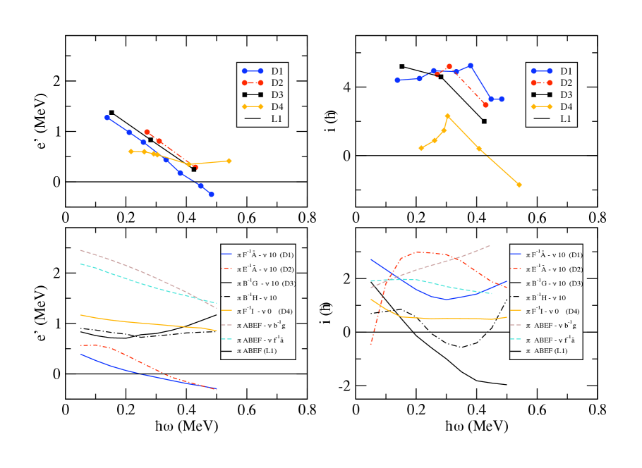
Figure 41: Experimental and calculated routhians and single-particle aligned angular momenta relative to band L1 for the $\Delta I=1$ bands D1-D4 in ¹³⁸Nd. The line type indicates the parity: full $\pi=+$, dash-dot $\pi=-$. The label $\nu 0$ means no neutron excitation and $\nu 10$ is short-hand for the neutron configuration B$\bar{\mathrm{A}}$. The calculated routhians, except $\pi ABEI\nu 0$, are shifted by $E_{exp,L6}(10^{+})-(E_{calc,\nu 10}(\omega=0)-E_{calc,\nu 0}(\omega=0))$ in order to account for the energy needed breaking a neutron pair. Taken from Ref. [107].

3.8.6 Tilted axis cranking solutions of triaxial nuclei

Triaxial deformation at moderate spin is predicted for the regions around $Z=44,~{}N=64$, $Z=64,~{}N=76$ and $Z=78,~{}N=116$ [106]. When the ${\cal R}_{z}(\pi)$ symmetry is broken, triaxial tilted axis cranking solutions are observed as $\Delta I=1$ bands, as it is the case for axial solutions. Fig. 40 shows the single particle routhians around $Z=60,~{}N=78$. The proton h_11/2 orbitals from the bottom of the shell drive toward $\vartheta=90^{\circ}$ because they have best overlap when aligned with the s-axis, while the neutron h_11/2 orbitals from the top of the shell drive toward $\vartheta=0^{\circ}$ because they have best overlap when aligned with the l-axis (see discussion in A). Combining them results in a tilt of the rotational axis into the s-l-plane. These configurations appear as $\Delta I=1$ dipole bands. Fig. 41 shows the dipole bands observed in ${}^{138}_{60}\mathrm{Nd}_{78}$ by Petrache et al. [107]. The routhians and alignments are displayed relative to the band L1, which is the proton configuration at $\vartheta=90^{\circ}$ with the routhians ABEF and below occupied and the neutron configuration at $\vartheta=0^{\circ}$ with the routhians A$\bar{\mathrm{A}}$EF and below occupied. This configuration has $\vartheta=90^{\circ}$ and appears as an even-$I$ band. The configurations of the dipole bands are labelled by the p-h excitations relative to L1, where $\nu 0$ means no neutron excitation and $\nu 10$ is short-hand for the neutron configuration B$\bar{\mathrm{A}}$. The relative routhians and aligned angular momenta are the sums of the excited particles and holes. Such simple scheme roughly accounts for the experiment and provides a configuration assignment. Better agreement with the experiment cannot be expected for a fixed deformation and zero pairing.

Wobbling

One important difference to axial nuclei is that for trixial nuclei the moments of inertia of all three principal axes are finite, which represent an additional degree of freedom: the orientation of the core angular momentum $\vec{R}$ with respect to the principal axes. It appears as low-energy collective quadrupole states which are generated by exciting rotational quanta about the axes with the smaller moments of inertia. They form the spectrum of the triaxial rotor Hamiltonian (7), which for molecules as water is observed up to a large number of quanta along the unfavored axes. In the case of nuclei, only the lowest excitations are realized, which have been called the wobbling mode [6]. Its presence is a clear indication of triaxiality. We discuss two phenomena, transverse wobbling and chiral vibrations, which appear as a consequence of the strong coupling of the wobbling mode with the quasiparticles.

For the discussion it is important to note that the moment of inertia of the collective core is largest for the m-axis. This is the case for the irrotational flow moments of inertia. Rotating mean field calculations confirm this order, which is also implied by the observation that the collective moment of inertia increases with the deviation from symmetry with respect to rotational axis. The deviation is largest for the m-axis, because the perpendicular l- and s-axes have largest length difference. In the following discussions we assign the s-axis to 1, the m-axis to 2 and the l-axis to 3.

The harmonic limit of wobbling has been discussed by Bohr and Mottelson [6], which we sketch. The yrast states with no wobbling excitation correspond to rotation about the 2-axis with the largest moment of inertia. The rotor Hamiltonian (7) is rearranged as

$$H=\frac{\hat{R}^{2}}{2{\cal J}_{2}}+H_{W},~{}~{}~{}H_{W}=R\left(\frac{1}{2{\cal J}_{3}}-\frac{1}{2{\cal J}_{2}}\right)\hat{r}_{3}^{2}+R\left(\frac{1}{2{\cal J}_{1}}-\frac{1}{2{\cal J}_{2}}\right)\hat{r}_{1}^{2}.$$ (109)

with $\hat{r}_{1}=\hat{R}_{1}/\sqrt{R}$ and $\hat{r}_{3}=\hat{R}_{3}/\sqrt{R}$. The rotor energy is minimal for uniform rotation about the 2-axis, which is given by the first term as $R(R+1)/(2{\cal J}_{2})$. It is assumed that the deviation of $\hat{R}_{2}$ from its eigenvalue $R$ is small such that $[\hat{R}_{3},\hat{R}_{1}]=-i\hat{R}_{2}\approx-iR$. Within this harmonic approximation, $\hat{r}_{1}$ and $\hat{r}_{3}$ are canonical operators and $H_{W}$ represents a harmonic oscillator with the spectrum

$$E_{W}=\hbar\omega_{W}(n+1/2),~{}~{}\omega_{W}=\frac{R}{{\cal J}_{2}}\sqrt{\left(\frac{{\cal J}_{2}}{{\cal J}_{3}}-1\right)\left(\frac{{\cal J}_{2}}{{\cal J}_{1}}-1\right)},$$ (110)

where $R$ has to be taken as $R+1/2$ in order to account for semiclassical corrections (cf. A). Wobbling means that the angular momentum vector precesses on an elliptic cone about the 2-axis. In the laboratory frame it corresponds to the same precession of the m-axis about the angular momentum vector $\vec{R}$. The wobbling phonon carries the signature $\alpha=1$ because $\hat{r}_{1}$ and $\hat{r}_{3}$ are odd under the rotation ${\cal R}_{2}(\pi)$. That is, the zero-phonon state has $\alpha=0$, the one-phonon state $\alpha=1$, and the two-phonon state $\alpha=0$. The expressions for the quadruple transitions matrix elements are given in Refs. [6] (section 4.5e) and [108].

The left panel of Fig. 42 shows the lowest bands in ${}^{112}_{44}$Ru₆₈ as the best example for this kind of ”simple” wobbling observed so far. The expected sequence even $I$, odd $I$, even $I$ for the respective zero-, one-, and two-phonon states is observed. However, only above $I=10$ one sees the expected increase of $\omega_{W}$ with $I$. The equidistance between the zero-, one- and two-phonon states, characteristic for the harmonic, limit is strongly perturbed.

Transverse wobbling

In axial nuclei the tilt of the rotational axis reflects the combination of quasiparticle angular momentum along the symmetry axis and collective angular momentum perpendicular to it, which increases along the band. As a consequence, the tilt angle $\vartheta$ increases with $\omega$. As discussed in section 3.8.5, this may lead to a transition from broken to restored ${\cal R}_{z}(\pi)$ symmetry (i. e. signature splitting) when $\vartheta$ approaches $90^{o}$. The analog can happen in triaxial nuclei when a quasiparticle aligns with the 1- or 3- axis causing a tilt of the rotational axis into the 1-2- or 1-3- planes, respectively. However, there is also the possibility of a transition from conserved to broken ${\cal R}_{z}(\pi)$ symmetry with increasing frequency. This occurs when a high-j particle couples to the triaxial core. As discussed in A, it aligns its angular momentum with the s-axis, because this orientation maximizes the overlap with the triaxial potential. When $\vec{R}$ aligns with the s-axis the energy gain due to the cranking term $-\vec{\omega}\cdot\vec{J}$ is maximal. With this orientation the ${\cal R}_{z}(\pi)$ symmetry is good, and the band is a $\Delta I=2$ sequence of good signature. When $\vec{R}$ has the direction of the m-axis the energy of the collective rotation is minimal. With this orientation the ${\cal R}_{z}(\pi)$ symmetry is broken, and the band is a $\Delta I=1$ sequence. The balance of these two energies decides the symmetry. Since the cranking term is linear and the collective rotational energy quadratic, the former dominates at low and the latter at high $\omega$.

The essence of the interplay is seen when one assumes that the angular momentum $j$ of the quasiparticle is rigidly aligned with the s-axis, which is the frozen alignment (FA) approximation studied in Ref. [108]. The classical routhian augmented by the Lagrangian multiplier $\lambda\omega^{2}/2$ is

$$E^{\prime}(\vec{\omega})+\lambda\omega^{2}/2=-\frac{1}{2}\sum\limits_{i}\omega_{i}^{2}{\cal J}_{i}-\omega_{1}j+\frac{1}{2}\lambda\sum\limits_{i}\omega_{i}^{2}.$$ (111)

The Lagrangian multiplier is added to find the stationary points under the constraint of fixed $\omega$, i. e. with respect to the orientation of the rotational axis. Taking the derivatives with respect to $\omega_{i}$ the stationary points are determined by the equations

$$({\lambda-\cal J}_{1})\omega_{1}=j_{1},~{}~{}({\lambda-\cal J}_{2})\omega_{2}=0,~{}~{}({\lambda-\cal J}_{3})\omega_{3}=0,$$ (112)

which have to be fulfilled simultaneously. The first solution

$$\omega=\omega_{1},~{}~{}\omega_{2}=0,~{}~{}\omega_{3}=0,~{}~{}\lambda={\cal J}_{1}+j/\omega$$ (113)

represents rotation about the 1-axis with

$$J={\cal J}_{1}\omega+j,~{}~{}E=\frac{(J-j)^{2}}{2{\cal J}_{1}}.$$ (114)

The second solution

$$\omega_{1}=\frac{j}{{\cal J}_{2}-{\cal J}_{1}}\equiv\omega_{c},~{}~{}\omega_{2}\not=0,~{}~{}\omega_{3}=0,~{}~{}\lambda={\cal J}_{2}.$$ (115)

represents rotation about an axis in the 1-2-plane tilted by the angle $\vartheta=\arctan(\omega_{1}/\omega_{2})$ with respect to the 1-axis. Energy and angular momentum are given by

$$J_{1}=\omega_{c}{\cal J}_{1}+j=\frac{j{\cal J}_{2}}{{\cal J}_{2}-{\cal J}_{1}}\equiv J_{c},~{}~{}J_{2}={\cal J}_{2}\omega_{2},~{}~{}~{}E=\frac{J_{c}^{2}}{2{\cal J}_{1}}+\frac{J^{2}-J_{c}^{2}}{2{\cal J}_{2}}.$$ (116)

For $J<J_{c}$ the first solution has lower energy and is a minimum. It has ${\cal R}_{1}(\pi)$ symmetry and represents a $\Delta I=2$ band with the signature of the aligned quasiparticle.

For $J>J_{c}$ the second solution has the lowest energy and is a minimum where the first becomes a saddle point. The second solution represents rotation about the tilted axis. It breaks the ${\cal R}_{1}(\pi)$ symmetry and is assigned to a $\Delta I=1$ band. Thus $J_{c}$ marks the transition from a $\Delta I=2$ band of given signature to a $\Delta I=1$ band.

The energy (116) has a similar form as Eq. (20) for a quasiparticle rigidly aligned with the symmetry axis of an axial nucleus. In this case ${\cal J}_{1}=0$ and $j=\hbar K$. The first solution (113) does not represent a band. The second solution (115) represents the $\Delta I=1$ sequence built on the band head state with $I=K=J_{c}/\hbar$ (cf. Eqs. (20,103)). With increasing angular momentum the quasiparticle may decouple from the 1-axis and reorient its $\vec{j}$ toward the 2-axis. This corresponds to a transition to ${\cal R}_{2}(\pi)$ symmetry, which is analog to the transition discussed in section 3.8.5 before.

The transition from solution 1 assigned to a $\Delta I=2$ band to solution 2 assigned to a $\Delta I=1$ band has to be gradual. That is, a second $\Delta I=2$ sequence of opposite signature must merge with the first. The second band is the transverse wobbling excitation, which has been introduced by Frauendorf and Dönau [108]. Let us discuss the transition in the framework of the harmonic frozen alignment approximation (HFA) [108], which considers a Hamiltonian that corresponds to the classical routhian (111),

$$H_{FA}=\sum\limits_{i}\frac{\hat{R}_{i}^{2}}{2{\cal J}_{i}}=\frac{(\hat{J}_{1}-j)^{2}}{2{\cal J}_{3}}+\frac{\hat{J}_{2}^{2}}{2{\cal J}_{2}}+\frac{\hat{J}_{1}^{2}}{2{\cal J}_{3}},$$ (117)

where the aligned angular momentum $j$ is assumed to be fixed (”frozen”). For $J<J_{c}$ rotation about the 1-axis is preferred. Assuming that the components $\hat{J}_{2}$ and $\hat{J}_{3}$ are small, one approximates $\hat{J}_{1}\approx J-\hat{J}_{2}^{2}/2J-\hat{J}_{3}^{2}/2J$. This leads to a harmonic wobbler Hamiltonian that looks like $H_{W}$ for the simple wobbler given by Eq. (109) when one changes the axes as $2\rightarrow 1,~{}3\rightarrow 2,~{}1\rightarrow 3$ and replaces

$$R\rightarrow J~{}~{}{\mathrm{and}}~{}~{}{\cal J}_{1}\rightarrow\bar{\cal J}_{1}=\frac{{\cal J}_{1}}{1-j/J}.$$ (118)

The resulting modified expression (110) can be rewritten as

$$\omega_{w}=\frac{j}{{\cal J}_{1}}\left[\left(1+\frac{J}{j}\left(\frac{{\cal J}_{1}}{{\cal J}_{2}}-1\right)\right)\left(1+\frac{J}{j}\left(\frac{{\cal J}_{1}}{{\cal J}_{3}}-1\right)\right)\right]^{1/2}.$$ (119)

For the considered case of transverse wobbling the quasiparticle’s angular momentum is aligned with the 1-axis, which means that ${\cal J}_{1}<{\cal J}_{2}$ and ${\cal J}_{1}>{\cal J}_{3}$. Then, the factor $1+J({\cal J}_{1}/{\cal J}_{2}-1)/j$ in Eq. (119) decreases with $J$ and the wobbling energy will also decrease for sufficiently large $J$. It reaches zero at $J_{c}$ the critical angular momentum (112).

Frauendorf and Dönau [108] classified the wobbling modes as transverse when the quasiparticle’s angular momentum is perpendicular to the m-axis and as longitudinal when it is aligned with the m-axis. A hole coupled to the triaxial core will align its angular momentum with the 3-axis (l-) which also corresponds to transverse wobbling. For the typical order ${\cal J}_{2}>{\cal J}_{1}>{\cal J}_{3}$ the decrease of $\omega_{W}$ with $J$ is more rapid than for the high-j particle as can be seen from Eq. (119) after exchanging the axes $1\leftrightarrow 3$. A mid-shell quasiparticle tends to align with the 2-axis (m-), which corresponds to longitudinal wobbling. The wobbling frequency increases with $J$, as can be seen from Eq. (119) after exchanging the axes $1\leftrightarrow 2$, because both factors increase with $J$.

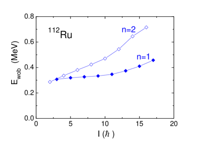
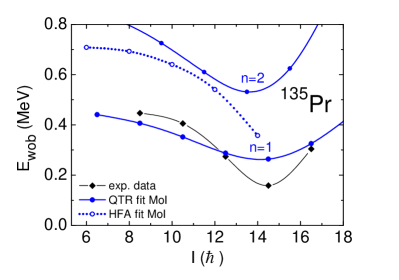
Figure 42: Left: Experimental energies of the two lowest wobbling bands $n=1$ (odd $I$) and $n=2$ (even $I$) relative to the $n=0$ yrast sequence in ¹¹²Ru as an example for a simple wobbler.
Right: Excitation energies of the $n=1~{}(\alpha=1/2)$ and $n=2~{}(\alpha=-1/2)$ of the $\pi h_{11/2}$ transverse wobbling bands relative to the $n=0~{}(\alpha=-1/2)$ yrast sequence in ¹³⁵Pr. Solid blue lines and full dots: quasiparticle triaxial rotor calculation (QTR); dotted blue lines and open dots: HFA calculation (119); black line and full diamonds: experimental data. From [108].

The right panel of Fig. 42 shows ${}^{135}_{59}$Pr₇₆ as an example for transverse wobbling. The yrast configuration is $[\pi(\mathrm{AEF})\nu(\bar{\mathrm{A}}\mathrm{AEF})]$ in the single routhian diagram Fig. 40. The calculations use ${\cal J}_{m}=21~{}\hbar^{2}\mathrm{MeV}^{-1},~{}{\cal J}_{s}=13~{}\hbar^{2}\mathrm{MeV}^{-1},~{}{\cal J}_{l}=4~{}\hbar^{2}\mathrm{MeV}^{-1}$, which were adjusted to optimize the agreement with the experimental energies. For the diagonalization of the full quasiparticle triaxial rotor Hamiltonian (37) a pure h_11/2 proton is assumed and a deformation of $\beta=0.17,\ \gamma=26^{\circ}$.

The orbital A is aligned with the s-axis which is transverse to the m-axis. Accordingly, the wobbling frequency decreases with $I$. The HFA expression (119) gives $\omega_{W}=0$ at the critical spin which is $J_{c}=14.4\hbar$ by Eq. (112). In addition the full quasiparticle + triaxial rotor (QTR) calculation (see section 2.7) is shown, to which HFA is an approximation that becomes invalid near and above $J_{c}$. In contrast to the HFA, the exact eigenvalues of $H_{QTR}$ (37) smoothly pass $J_{c}$. The h_11/2 quasiproton is not rigidly aligned with the s-axis. The quasiparticle triaxial rotor model takes into account its response to the inertial forces by gradually tilting $\vec{j}$ toward the m-axis. For the considered case this realignment is substantial, such that for $J>J_{c}$ longitudinal coupling becomes prevalent, which is seen as the increase of the wobbling frequency.

Wobbling is a motion of the triaxial charge density relative to the space fixed angular momentum vector, which generates enhanced E2 radiation. Frauendorf and Dönau [108] predicted large $B(E2,I\rightarrow I-1)$ values for the transitions from the wobbling to the yrast band, which were confirmed by Matta et al. [110]. These strong E2 transitions discriminate the wobbling band against the signature partner band with the configuration $[\pi(\mathrm{BEF})\nu(\bar{\mathrm{A}}\mathrm{AEF})]$ in Fig. 40, which has the same signature $\alpha=1/2$ as the wobbling band. The pertinent band was also identified in addition to the wobbling and found to have the expected weak E2 transitions to the yrast band.

Frauendorf and Dönau [108] calculated microscopic moments of inertia ${\cal J}_{m}=17~{}\hbar^{2}\mathrm{MeV}^{-1},~{}{\cal J}_{s}=7~{}\hbar^{2}\mathrm{MeV}^{-1},~{}{\cal J}_{l}=3\hbar^{2}~{}\mathrm{MeV}^{-1}$ by means of cranking with small $\omega$ about the three principal axes. For these values Eq. (112) gives the critical spin $J_{c}=9.3\hbar$, which is lower than 14.4$\hbar$ obtained with the fitted moments of inertia. A direct tilted axis cranking calculation using the same parameters gives $\vartheta=90^{\circ}$ and $\varphi=0$ for low $\omega$, i. e. rotation about the s-axis. Above $\hbar\omega_{c}=0.28$ MeV the tilt angle $\varphi$ moves rapidly toward $90^{\circ}$, i.e. the rotational axis swipes through the s-m-plane. The critical frequency is smaller than $\hbar\omega_{c}=0.55$ MeV obtained by means of the HFA expression (115) for the cranking moments of inertia. Possible reasons for the discrepancy may be that the quasiproton is not rigidly aligned with the s-axis and that the moments of inertia are not constant up to $\omega_{c}$ as assumed in the estimate (115). Transverse wobbling appears to be rather sensitive to the value of $\gamma$ and of the pair gaps $\Delta$, which strongly influence the ratios between the three moments of inertia. The sensitivity to such details makes it difficult obtaining precise results by microscopic calculations. However, for transverse wobbling of the triaxial strongly deformed ^163,165,157Lu isotopes, the microscopic calculations that combined principal axis cranking with quasiparticle random phase approximation (see section 2.5) provided quite promising results [111, 112]. In their contribution to this Focus Issue, Sheikh et al. [58] present the microscopic study of transverse wobbling in ¹³⁵Pr in the framework of the Triaxial Projected Shell Model, which describes the wobbling energy as well as the quasiparticle triaxial rotor model calculation in shown in Fig. 42 right. I. Hamamoto discusses wobbling in her contribution to this Focus Issue as well [109].

Chirality

When the angular momentum does not not lie in one of the three principal planes of a triaxial nucleus the combination of the three different principal axes with $\vec{J}$ becomes chiral (see section 3.2). There are the left-handed $|l\rangle$ and right-handed $|r\rangle$ mean field solutions, which a related to each other by

$$|l\rangle={\cal TR}_{y}(\pi)|r\rangle.$$ (120)

In the ideal case of strongly broken ${\cal TR}_{y}(\pi)$ symmetry, the matrix elements $\langle l|Q_{22}|r\rangle,~{}\langle l|Q_{21}|r\rangle$ and $\langle l|\mu_{11}|r\rangle$ are small because the electromagnetic field does not provide enough angular momentum to turn the long vector $\vec{J}$ from the left- to the right-handed position. In order to calculate the transition matrix elements for this ideal case one must take into account that the exact states of the two bands have good ${\cal TR}_{y}(\pi)$ symmetry. One may choose the phases such that

$${\cal TR}_{y}(\pi)|IM\pm\rangle=|IM\pm\rangle$$ (121)

when acting on the states $|IM\pm\rangle$ of good angular momentum, which describe the two degenerate bands (see Ref. [13]). The linear combinations

$$|+\rangle=\frac{1}{\sqrt{2}}(|r\rangle+|l\rangle),~{}~{}|-\rangle=\frac{i}{\sqrt{2}}(|r\rangle-|l\rangle)$$ (122)

fulfill the relation (121), i. e. they restore the broken symmetry. Thus for $E2$-transitions one has instead of (75)

$$B(E2,I~{}\pm\rightarrow I-2~{}\pm)=\frac{5}{8\pi}|\langle r|Q_{22}|r\rangle+\langle l|Q_{22}|l\rangle|^{2},$$ (123)

$$B(E2,I~{}\pm\rightarrow I-2~{}\mp)=\frac{5}{8\pi}|\langle r|Q_{22}|r\rangle-\langle l|Q_{22}|l\rangle|^{2}$$ (124)

Eqs. (76) and (69) are modified in the same way [113].

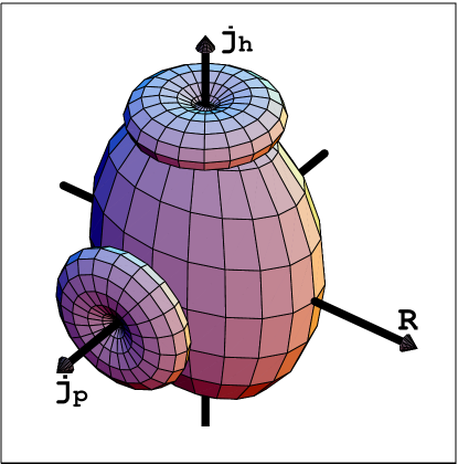
Figure 43: Orbitals of a high-$j$ proton and a high-$j$ neutron hole coupled to the triaxial density distribution. The collective angular momentum $\vec{R}$ of the rotor prefers the medium axis, which has the largest moment of inertia. The total angular momentum $\vec{J}=\vec{R}+\vec{j}_{p}+\vec{j}_{h}$ points out of the plane of the drawing. The short, medium and long axes form a right-handed screw with respect to $\vec{J}$.

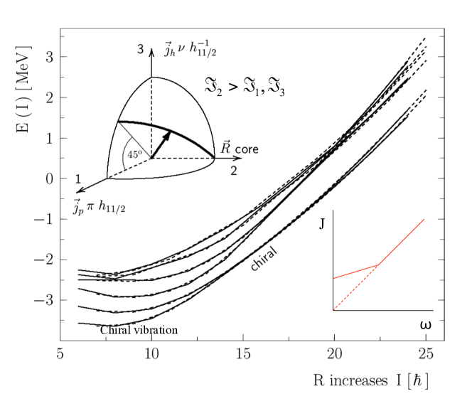
Figure 44: Rotational levels of a $\pi h_{11/2}$ particle and a $\nu h_{11/2}$ hole coupled to a triaxial rotor with $\gamma=30^{o}$. Full lines: $\alpha=0$ (even $I$). Dashed lines to $\alpha=1$ (odd $I$). The left inset shows the orientation of the angular momentum with respect to the triaxial potential, where 1, 2 and 3 correspond to the s-, m- and l- axes, respectively. The angular momentum vector moves along the heavy arc. The position displayed corresponds to the spin interval $13<I<18$, where the two lowest bands are nearly degenerate. The right-handed position is shown. The left-handed is obtained by reflection through the 1-3 plane. The calculation uses $\varepsilon=0.24$, $\gamma=30^{\circ}$ and the irrotational-flow ratio ${\cal J}_{2}/{\cal J}_{1,3}=4$. The right inset shows the function $J(\omega)$ for the frozen alignment approximation. Adapted from Ref. [115].

The ${\cal TR}_{y}(\pi)$ symmetry is broken when the angular momentum has components on all three principal axes. Fig. 43 illustrates the typical angular momentum geometry. High-j particles of one kind of nucleons and high-j holes of the other kind couple with the triaxial deformed potential. The particles tend to align their angular momentum with the short axis and the holes with the long axis, because these orientations maximizes the overlap of their density distributions with the potential (see A). The collective angular momentum $\vec{R}$ provides the third component along the medium axis. In analogy to transverse wobbling, the collective angular momentum $\vec{R}$ increases along the band. At the band head, only the particle and the hole generate the angular momentum, which lies in the 1-3 plane. At low frequency, $\vec{R}$ stays within this s-l- plane aligning with the angular momentum of the particle and hole, because this orientation minimizes the cranking term $-\vec{\omega}\cdot\vec{J}$. For larger values of $\omega$ it is energetically favorable that $\vec{R}$ increases into the direction of the m-axis, because the moment of inertia is larger. The vector $\vec{J}$ moves out of the 1-3 plane towards the 2-axis. Accordingly the symmetry changes from ${\cal R}_{z}\not=1,~{}{\cal TR}_{y}=1$, corresponding to one $\Delta I=1$ band, to ${\cal R}_{z}\not=1,~{}{\cal TR}_{y}\not=1$, corresponding to two degenerate $\Delta I=1$ bands. As for transverse wobbling, there is a critical frequency for which the planar tilted axis cranking solution becomes chiral.

To qualitatively discuss the transition we use again the frozen alignment approximation, i. e. we assume that the particle angular momentum $j_{1}$ is rigidly aligned with the 1-axis (s-) and the hole angular momentum $j_{3}$ with the 3-axis (l-). To find the stationary points with respect to the orientation of $\vec{\omega}$ the classical routhian is augmented by the Lagrangian multiplier $\frac{1}{2}\lambda\omega^{2}$ in order to keep $\omega^{2}$ constant,

$$E^{\prime}(\omega_{1},\omega_{2},\omega_{3})+\frac{1}{2}\lambda\omega^{2}=-\frac{1}{2}\sum\limits_{i}{\cal J}_{i}\omega^{2}_{i}-\omega_{1}j_{1}-\omega_{3}j_{3}+\frac{1}{2}\lambda\sum\limits_{i}\omega_{i}^{2}.$$ (125)

Taking the derivatives with respect to $\omega_{i}$, the stationary points are given by the equations

$$({\lambda-\cal J}_{1})\omega_{1}=j_{1},~{}~{}({\lambda-\cal J}_{2})\omega_{2}=0,~{}~{}({\lambda-\cal J}_{3})\omega_{3}=j_{3},$$ (126)

which have to be fulfilled simultaneously [89]. As for transverse wobbling, there are two solutions, which are determined by second equation. The solution is planar when $\omega_{2}=0$, or chiral when $\lambda={\cal J}_{2}$. For the chiral solution $\omega_{2}$ increases while the other two components stay constant $\omega_{1}=j_{1}/({\cal J}_{2}-{\cal J}_{1})$ and $\omega_{3}=j_{3}/({\cal J}_{2}-{\cal J}_{3})$. At the critical frequency $\omega_{c}$ both $\omega_{2}=0$ and $\lambda={\cal J}_{2}$, which means

$$\omega_{c}=\sqrt{\left(\frac{j_{1}}{({\cal J}_{2}-{\cal J}_{1})}\right)^{2}+\left(\frac{j_{3}}{({\cal J}_{2}-{\cal J}_{3})}\right)^{2}},~{}~{}J_{c}={\cal J}_{2}\omega_{c}.$$ (127)

As in the case of transverse wobbling, the chiral doubling develops in a gradual way. Below $J_{c}$ the second $\Delta I=1$ band appears as the one-phonon chiral vibration excitation. Frauendorf and Dönau [114] worked out the small amplitude solution of the frozen alignment approximation. The expressions are too complex to be included here. Frauendorf and Meng [115] carried out quasiparticle triaxial rotor model calculations for the special case $j_{1}=j_{2}=11/2$ and $\gamma=30^{\circ}$, which are shown in Fig. 44. The irrotational-flow ratios of the moments of inertia were assumed, which are ${\cal J}_{2}/{\cal J}_{1}={\cal J}_{2}/{\cal J}_{3}=4/1$. According to the frozen alignment estimate (127), the one-phonon band merges the zero-phonon band at $J_{c}=\sqrt{2}j_{1}{\cal J}_{2}/({\cal J}_{2}-{\cal J}_{1})=\sqrt{2}\times 11/2\hbar\times 4/3=10.3\hbar$. In the full quasiparticle triaxial rotor calculation, the two bands meet somewhat above at $J=14\hbar$. Based on their quasiparticle triaxial rotor model, the authors realized for the first time that the doublets manifest the left-handed and right- handed geometry of the three types of angular momentum illustrated in Fig. 43. They suggested that the two $\Delta I=1$ sequences observed in ${}^{134}_{59}$Pr₇₅ represent chiral partner bands.

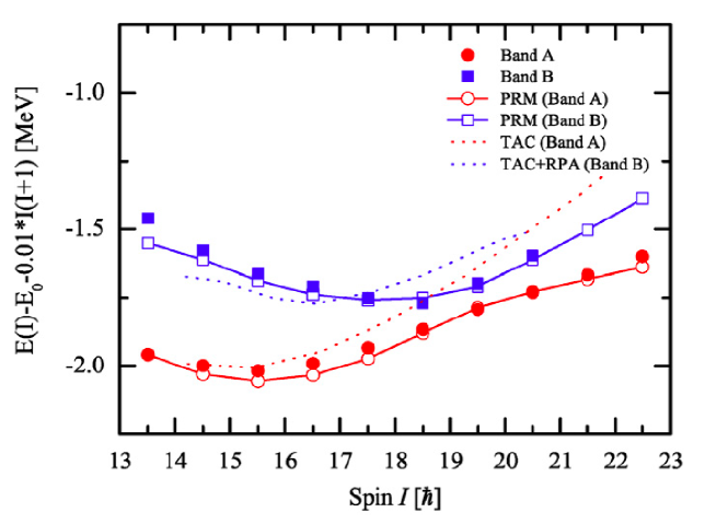
Figure 45: The excitation energies $E(I)$ for the chiral sister bands in ¹³⁵Nd with the configuration $[\pi h_{11/2}^{2}\nu h_{11/2}^{-1}]$. Filled symbols: experiment [117, 118]; open symbols (PTR): two protons+one neutron hole+triaxial rotor ($\gamma=30^{\circ}$) calculations; dotted lines: TAC +QRPA calculations [117, 118]. Taken from Ref. [119].

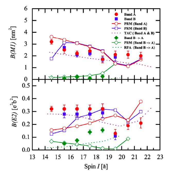
Figure 46: Reduced transition probabilities of the chiral sister bands in ¹³⁵Nd with the configuration $[\pi h_{11/2}^{2}\nu h_{11/2}^{-1}]$. Filled symbols: experiment [117, 118]; open symbols (PRT): two protons+one neutron hole+triaxial rotor ($\gamma=30^{\circ}$) calculations; dotted lines (TAC): inband transitions calculated by means of TAC; dotted lines (RPA): interband transitions calculated by means QRPA based on the TAC mean field [117, 118]. Taken from Ref. [119].

Dimitrov et al. [113] found the first chiral rotating mean field solution in the framework of shell correction tilted axis cranking approach (SCTAC) for ${}^{134}_{59}$Pr₇₅. The configuration is composed of a particle-like $h_{11/2}$ quasiproton and a hole-like $h_{11/2}$ quasineutron. Without pairing the configuration is $[\pi AEF\nu A]$ in Fig. 40, which has a finite tilt $\vartheta$ in the s-l-plane. The collective angular momentum $\vec{R}$ drives the rotational axis out of the s-l-plane at the critical spin $J_{c}=10.7\hbar$ corresponding to $\hbar\omega_{c}=0.30$ MeV ($\vartheta=60^{\circ}$ and $\beta=0.19,~{}\gamma=28^{\circ}$). The result is consistent with the observed encounter of the two $\Delta I=1$ sequences at $I=14$. The encounter is actually a crossing of the two sequences, which depart from each other for higher spin. Almehed et al. [116] described the excited $\Delta I=1$ bands in odd-odd nuclei around $A=134$ as the one-phonon chiral vibrational excitations in the framework of the QRPA (see section 2.5) based on the planar rotating mean field solution found by SCTAC (TAC+QRPA). The method provides the vibrational energy $\hbar\omega_{V}$ without any new parameter. In case of ¹³⁴Pr, the value of $\hbar\omega_{V}=0.30$ MeV at the rotational frequency $\hbar\omega$=0.30 MeV is somewhat lower than the experimental value of 0.37 MeV. The QRPA values stay below the experimental ones, reaching zero at $J_{c}$.

Figs. 45 and 46 shows ${}^{135}_{60}$Nd₇₅ as another example for the transition from the planar to a chiral mean field solution. The configuration is composed of two particle-like $h_{11/2}$ quasiprotons and a hole-like $h_{11/2}$ quasineutron. Without pairing the configuration is $[\pi ABEF\nu A]$ in Fig. 40, which has a finite tilt $\vartheta$ in the s-l-plane. In the SCTAC calculations carried out by Zhu et al. [117], the collective angular momentum $\vec{R}$ drives rotational axis out of the s-l-plane at the critical spin $J_{c}=20.5\hbar$ corresponding to $\hbar\omega_{c}=0.47$ MeV ($\vartheta=68^{\circ}$ and $\varepsilon\approx 0.20,~{}\gamma\approx 30^{\circ}$). In the experiment the two partner bands come closest at $J=(I+1/2)\hbar=20\hbar$. In order to describe the approach of the one-phonon band Mukhopadhyay et al. [118] carried out TAC+QRPA calculations along the lines described in Ref. [116]. As seen in Fig. 45, the calculation well reproduces the experiment without any parameter adjustment up to $J_{c}$ where the QRPA stops working. Fig. 46 shows that the TAC+QRPA calculations reproduce the $B(M1)$ and $B(E2)$ values of the two bands fairly well. Qi et al. [119] studied the transition from chiral vibration to chiral rotation in the framework of the quasiparticle particle triaxial rotor model (cf. section 2.7). Two $h_{11/2}$ protons and one $h_{11/2}$ neutron hole were coupled to a triaxial rotor with irrotational-flow ratios between the moments of inertia. The model parameters, the average value of the moments of inertia, the triaxiality parameter $\gamma$ and the coupling strength to the deformed potential, were adjusted to reproduce the experimental energies. The results in Figs. 45 and 46 rather well account for the experiment. The analysis of the angular momentum geometry showed that around $J=20$ the two bands are to good approximation represented by the two linear combinations (122). Above, the two bands move apart again because the two protons are tilted toward the m-axis like the one proton generating transverse wobbling in the neighbor ${}^{135}_{59}$Pr₇₆ (see discussion above).

Alcántara-Núñez et al. [120] and Timár et al. [121] found two chiral tilted axis cranking solutions in the same nucleus ${}^{105}_{45}$Rh₆₀, which belongs to the second region of triaxiality around $Z=44,~{}N=64$. The tilt into the s-l-plane is generated by the combination of the hole-like $g_{9/2}$ quasiproton with particle-like $h_{11/2}$ quasineutrons. For the configuration $[\pi g_{9/2}\nu h_{11/2}^{2}$] the tilted axis cranking solutions becomes chiral at $J_{c}=21\hbar$ ($\vartheta=75^{\circ},~{}\beta=0.23,~{}\gamma=29^{\circ}$, SCTAC). The pertinent experimental bands approach each other like for the discussed $A=134,$ 135 cases. At $I=45/2$ the distance reaches its minimum of 100 keV. For the second configuration [$\pi g_{9/2}\nu h_{11/2}(g_{7/2}d_{5/2})$] the tilted axis cranking solution becomes chiral at $J_{c}=9\hbar$ ($\vartheta=57^{\circ},\beta=0.23,~{}\gamma=29^{\circ}$). The pertinent bands are nearly degenerate for $I=17/2$ and 19/2 ($\Delta E<$50 keV). For larger spin the partners depart from each other as in the case of ${}^{134}_{59}$Pr₇₅. Ayangeakaa et al. [122] found two chiral bands in ¹³³Ce with the configurations $[\pi\mathrm{g}^{-1}_{7/2}\pi\mathrm{h}^{1}_{11/2}\nu\mathrm{h}^{-1}_{11/2}]$ and $[\pi\mathrm{h}^{2}_{11/2}\nu\mathrm{h}^{-1}_{11/2}]$.

Zhu et al. [123] and Luo et al. [124] interpreted a pair of bands in the even - $N$ Mo and Ru isotopes as chiral partners with a structure that differs from the one discussed so far. The suggested configuration is $[\nu\mathrm{h}_{11/2}^{1}(\mathrm{d}_{5/2}\mathrm{g}_{7/2})^{-1}]$. The tilted axis cranking calculations showed that the angular momentum of the normal parity $(d_{5/2}g_{7/2})$ hole is strongly aligned with the l-axis and the angular momentum of the $h_{11/2}$ with the s- axis. The total angular momentum moves from the l-s-plane through the aplanar region to the s-m-plane, which is caused by the collective angular momentum driving toward the m-axis. For $Z\approx 44$, $N\approx 66$ the two-quasineutron configuration $[h_{11/2}(d_{5/2}g_{7/2})]$ with $\Delta_{n}=0.7$ MeV was assumed [124]. The rotating mean field solution stayed in the s-l-plane being very soft in the m-direction. The TAC+QRPA calculations gave a vibrational frequency of about $300$ keV. The experimental bands in ${}^{106}_{42}$Mo₆₄ and ${}^{110,112}_{44}$Ru_66,68 are separated by about 200 keV or less and have similar decay properties, which qualifies them as chiral partners.

The dynamics of chirality beyond the harmonic approximation have mainly been studied in the framework quasiparticle triaxial rotor model model. The details of the approach relevant to chirality are presented in the contributions by K. Starosta and T. Koike [125] and I. Hamamoto [109] to this Focused Issue, which also contain a comprehensive review of the experimental evidence for chirality. Meng et al. [126] reviewed work on chirality from a more general perspective. The studies of doublet bands in odd-odd ^104,106Rh,^104,106Ag and ^98,100Tc in the framework of the Triaxial Projected Shell Model [127, 58] represent a promising perspective for a microscopic large-amplitude description of chiral doubling.

4 Emergence and disappearance of collective degrees of freedom

The Unified Model bases on the dichotomy of the ”collective” degrees of freedom, which describe the shape of the nucleus and the ”intrinsic” degrees of freedom, which are particle-hole configurations or quasiparticle configurations. Any number of collective excitations can be superimposed on the fermionic intrinsic states. Clearly this is an idealization. Nuclei are composed of a relative small number of nucleons compared to other many-body systems. The ”granular structure” of the collective degrees of freedom appears after the excitation of a finite number of quanta, which results in a progressive decoherence of the collective modes. This section is devoted to phenomena that require a refinement of the concept of the collective degrees of freedom. The focus will be on the rotational degrees supplemented by some thoughts about the $\beta$ degree of freedom.

As a condition for the appearance of rotational bands in nuclei, Bohr and Mottelson [6] state: ”A common feature of systems that have rotational spectra is the existence of a “deformation”, by which is implied a feature of anisotropy that makes it possible to specify an orientation of the system as a whole. In a molecule, as in a solid body, the deformation reflects the highly anisotropic mass distribution, as viewed from the intrinsic coordinate frame defined by the positions of the nuclei. In the nucleus, the rotational degrees of freedom are associated with the deformations in the nuclear equilibrium shape that result from the shell structure.” The first statement is very general, providing for all kinds of mechanisms that break the symmetry. The low spin data seemed to indicate that the only possibility to meet this condition is a substantial deformation of the nuclear density distribution, which is measured by the electric quadrupole moment. One suggestive evidence is the correlation between the moment of inertia and the nuclear deformation pointed out by Grodzin [102]. Raman et al. [103] found that ratio of the moment of inertia and the reduced probability for the $0^{+}\rightarrow 2^{+}$ transition can be well approximated by the expression

$$RJB(2^{+})=\frac{\cal J}{B(E2,0^{+}\rightarrow 2^{+})}=\frac{3}{E(2^{+})B(E2,0^{+}\rightarrow 2^{+})}$$

$$\approx 1150Z^{-2}A^{2/3}\hbar^{2}\mathrm{MeV}^{-1}(e\mathrm{b})^{-2},$$ (128)

where $E(2^{+})=3\hbar^{2}/{\cal J}$ is used. The ratio is nearly constant because both the numerator and the denominator are proportional to the square of the deformation. In the following we discuss phenomena that can only be understood by invoking the granular structure of nuclear rotation reflecting its microscopic underpinning.

4.1 Band termination

Band termination appears naturally within the clockwork picture of the rotating nucleus. Consider a nucleus that is not too strongly deformed, such that the grouping of the single-particle levels into spherical shells still exists. The angular momentum of the high-j orbitals remains close to $j$, their value in the spherical potential. The total angular momentum $J$ is generated by gradually aligning the angular momentum vectors $\vec{j}$ of the particles and holes in the incompletely filled shells. Eventually all vectors $\vec{j}$ are aligned in accordance with the Pauli principle. The mean field state $|\rangle$ is ${\cal R}_{z}(\psi)$-symmetric for this stretched coupling. That is, the band is terminated. In order to increase the angular momentum further, new configuration must be generated by exciting particles from the core. The shape may change appreciably before attaining ${\cal R}_{z}(\psi)$ symmetry at termination.

Experimentally, band termination is seen as a break of the smooth relation $J(\omega)$ between angular momentum and rotational frequency. Unlike after a band crossing, where another smooth sequence $J(\omega)$ starts, after a termination the level distances become irregular and there are competing parallel decay paths.

Termination may occur also for nuclei with a substantial deformation. Nucleons in a deformed harmonic oscillator potential, which rotates about a principal axis, is an illustrative example. Band termination within this model was comprehensively discussed by Afanasjev et al. [84], who also gave the pertaining references to the numerous earlier studies. The rotating harmonic oscillator separates into independent oscillations along the three principal axes, as the non-rotating oscillator does. A band is defined by a fixed number of oscillator quanta along each of the principal axes. Consider rotation about the 1-axis. The maximal angular momentum of a given configuration is

$$J_{1,max}=|\Sigma_{2}-\Sigma_{3}|,~{}~{}\Sigma_{2}=\sum\limits_{k,occ}\left(n_{2,k}+\frac{1}{2}\right),~{}~{}\Sigma_{3}=\sum\limits_{k,occ}\left(n_{3,k}+\frac{1}{2}\right),$$ (129)

where $n_{2,k}$ and $n_{3,k}$ are the numbers of quanta on the respective 2-, 3- axes of the single particle state $k$. When this value is reached the density becomes symmetric with respect to the 1-axis and the band terminates. Again, termination is due to of the restriction of the accessible angular momentum by quantization.

Termination does not have to take place. For near spherical nuclei, the deformation may change in such a way that the spherical shell structure dissolves. Then core angular momentum becomes accessible in addition to the angular momentum of the valence particles. For the harmonic oscillator [84] Afanasjev et al. delineated the shapes which terminate and which not.

The two mechanisms idealize different features of real nuclei. The high-j intruder orbitals behave like spherical ones whereas the low-spin orbitals are better accounted for by the deformed harmonic oscillator. Only realistic self consistent cranking calculations are capable of describing band termination quantitatively.

Bohr and Mottelson discussed band termination for light nuclei in the $sd$ shell [6]. Röpke and Endt [104, 105] used mean field configurations for classifying many bands, which all terminate when the amount of angular momentum available for the particles in the $sd$ shell is exhausted. The oscillator model accounts fairly well for the termination of bands in these light nuclei.

Nilsson and Ragnarsson [22] and Afanasjev et al. [84] reviewed the theoretical and experimental work on band termination in heavier nuclei. It commonly appears in nuclides with several valence particle or holes outside closed shells. A large number of terminating bands have been observed in the regions $Z\geq 64,~{}N\geq 82$ and $Z\approx 50,~{}N\approx 50$. Extensive theoretical analyses have been carried out in the frame of the Cranked Nilsson-Strutinsky (CNS) model (see section 3.7) as well as by means of configuration-confined selfconsistent approaches that are based on energy density functionals.

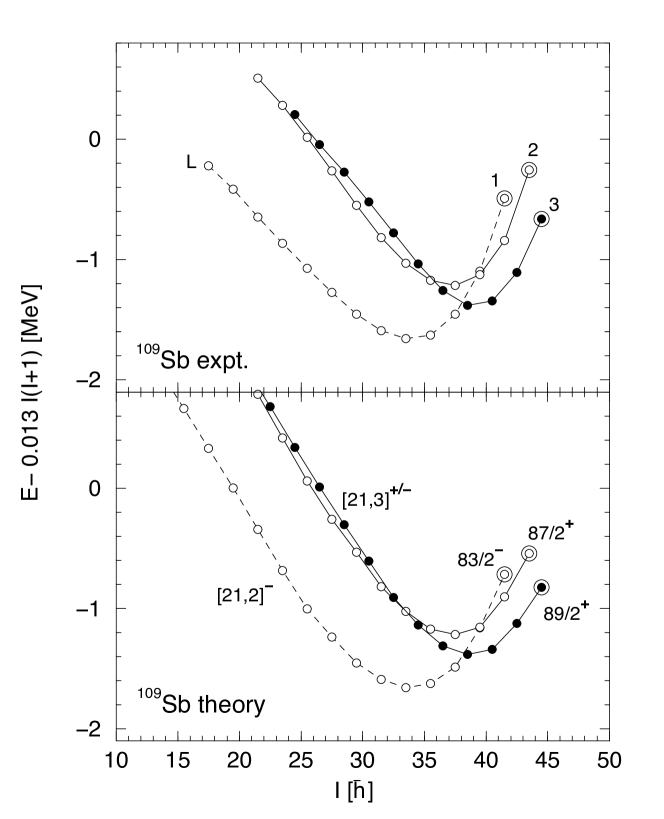
Figure 47: The energies of the bands 1, 2, 3 in ${}^{109}_{51}$Sb₅₈ relative to the energy of a rigid rotor with a moment of inertia of ${\cal J}=38\hbar^{2}\mathrm{MeV}^{-1}$. The terminating states are shown as large circles labeled by the spin and parity $I^{\pi}$. Band 2 and 3 are not linked to the known part of the spectrum. The unknown energy of the lowest level is chosen to give agreement with the Cranked Nilsson-Strutinsky calculations in the lower panel. The configuration assignment $[lm,n]^{\pm}$ in the lower panel is as follows. l: number of $g_{9/2}$ proton holes, m: number of $h_{11/2}$ proton particles, n: number of $h_{11/2}$ neutron particles and $\pm$ gives the signature $\alpha=\pm 1/2$. From Ref. [84]

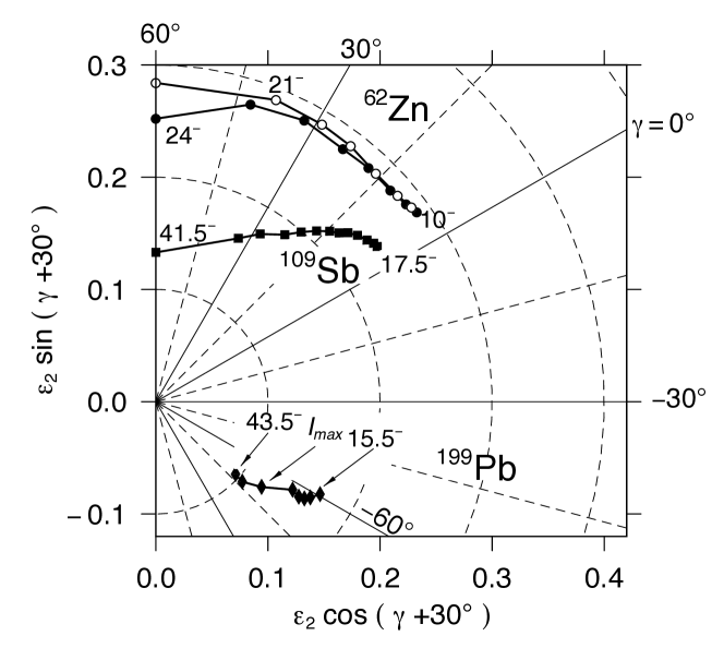
Figure 48: The calculated deformation parameters $\varepsilon(=\varepsilon_{2})$ and $\gamma$ of bands in ${}^{199}_{82}$Pb₁₁₇, ${}^{109}_{51}$Sb₅₈ and ${}^{62}_{30}$Zn₃₂ as functions of the angular momentum. Each spin value is represented by a symbol, where $\Delta I=2$. From Ref. [128].

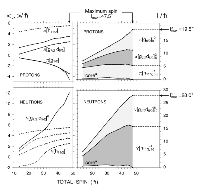
Figure 49: Contributions of the valence particles and holes to the total angular momentum of a terminating band in ${}^{111}_{51}$Sb₆₀. The calculations follow the deformation path relevant for the specific configuration, which is shown in Fig. 48. From Ref. [84]

As an example, Fig. 47 shows three terminating bands in ${}^{109}_{51}$Sb₅₈. Band 1 with $(\pi,\alpha)=(-,-1/2)$ has the proton configuration $[(g_{9/2})^{-2}_{8}(d_{5/2}g_{7/2})^{2}_{6}(h_{11/2})^{1}_{11/2}]$ and the neutron configuration $[(h_{11/2})^{2}_{10}(d_{5/2}g_{7/2})_{12}^{6}]$ relative to the $Z=N=50$ closed shell configuration. Stretched coupling of all the angular momenta gives $I^{\pi}=83/2^{-}$, as observed. The bands 2 and 3 with $(\pi,\alpha)=(+,-1/2)$ and $(+,1/2)$ have the same proton configuration combined with neutron configurations $[(h_{11/2})^{3}_{27/2}(d_{5/2}g_{7/2})_{21/2}^{5}]$ and $[(h_{11/2})^{3}_{27/2}(d_{5/2}g_{7/2})_{23/2}^{5}]$, respectively. As expected, they terminate at $I^{\pi}=87/2^{+}$ and $89/2^{+}$. Fig. 48 shows that band 1 starts with the substantial prolate deformation of $\varepsilon\approx 0.25$. Generating angular momentum by gradual alignment of the valence particle angular momenta, the shape becomes triaxial and then oblate and symmetric with respect to $\vec{J}$ at termination. The corresponding decrease of the $B(E2)$ values has been confirmed experimentally and agrees well with the Cranked Nilsson-Strutinsky (CNS) calculations [129, 84]. The dispersion $\Delta J$, which measures the symmetry breaking (see Sec. 4.4) and the moment of inertia ${\cal J}^{(2)}$ decrease along this path. The path in the $\varepsilon-\gamma$ plane is similar for bands 2 and 3.

Wadsworth et al. [129] and Afanasjev et al. [84] compare the CNS energies to the ones of a rotor with the rigid body moment of inertia, which has become the common way to present the data and calculations. They call the characteristic U-shape of the function $E(I)-E(I)_{rotor}$ in Fig. 47 a ”smooth unfavored termination”. ”Smooth” is just one of the criteria for a sequence of levels to qualify for a rotational band. The possibility to observe the bands up to termination is due to the low level density, which is caused by the gaps in the single-particle spectrum at $Z=50$ and $N=58$. If such gaps appear the smoothness condition is well satisfied (cf. Eq. (153) in section 4.4). ”Unfavored” means that the rotational energy is larger than that of the reference rotor. This feature, which is seen in Fig. 47 as the sharp increase of the relative energy at the highest spins, reflects the decrease of the moment of inertia ${\cal J}^{(2)}$.

Fig. 47 is an exampled for the general behavior of the terminating bands in the mass 110 region and lighter nuclei. Afanasjev et al. [84] characterize it as starting with ”collective rotation” and then ”gradually losing the collectivity”. In this way they describe the gradual restoration of the ${\cal R}_{z}(\psi)$ symmetry, which is substantially broken at the bottom of the band. This terminology is quite commonly used in connection with the appearance or disappearance of regular rotational sequences. It is discussed in detail in section 4.4 that the substantial symmetry breaking does not necessarily imply ”high collectivity” in the sense of a large number of nucleons being involved. Fig. 49 demonstrates that the rotation is not very collective. The angular momentum is generated by a relatively small number of particles. In the case of shears bands discussed in section 4.2 the number of active nucleons is 4-6. A more general and appropriate terminology is to characterize termination as a gradual loss of coherence of the rotational motion.

4.2 Magnetic rotation

As already discussed in section 3.8.2 the orientation of the nuclear mean field is to be attributed to the arrangement of the nucleonic orbitals, in particular the strongly un-isotropic high-j orbitals. The discovery of Magnetic Rotation is a striking example for this picture of a spinning clockwork of gyroscopes. In 1991 Baldsiefen et al. [131] and Fant et al. [130] reported the observation of very regular pattern of $\gamma$ rays in ^197-200Pb, which can be arranged into rotational bands according to the accepted criteria. At low spin irregular level spacings are observed that are typical for these semi magic nuclei with a near spherical shape. The regular band structures appear for $I>10$. The moments of inertia are ${\cal J}^{(2)}\sim 20\hbar^{2}MeV^{-1}$, about one half of the moments of inertia of the $2^{+}$ states of the well deformed nuclei of the rare earth region. However, the transitions were shown to be of stretched dipole type and arguments in favor of a magnetic character were presented. The weak or missing stretched $E2$-transitions pointed to the very small deformation expected for these nuclei. The observation, completely unexpected in the context of the Unified Model, was explained by Frauendorf [87] by means of TAC calculations. Reviews on Magnetic Rotation are given in Refs. [14, 133, 134, 135] and in the contribution by Meng and Zhao to this Focus Issue [42].

The experimental results are in contradiction with the traditional Unified Model view, according to which nuclear rotation is a collective phenomenon which only occurs in well deformed nuclei. The ratio ${\cal J}^{(2)}/B(E2,0^{+}\rightarrow 2^{+})$, which is $\sim 10(eb)^{-2}\hbar^{2}\mathrm{MeV}^{-1}$ for well deformed heavy nuclei and $\sim 5(eb)^{-2}\hbar^{2}\mathrm{MeV}^{-1}$ for superdeformed nuclei, exceeds $100(eb)^{-2}\hbar^{2}\mathrm{MeV}^{-1}$ for the dipole bands. There must be something rotating that carries a long transverse magnetic dipole moment but almost no charge quadrupole moment.

Figs. 50 illustrates the structure this novel rotor, which is an example that few high-j orbitals establish sufficient orientation such that quantal rotation emerges. As a typical case let discuss the magnetic dipole band 2 in ${}^{199}_{82}$Pb₁₁₇, which is illustrated in Fig. 51 in more detail. A pair of protons is excited across the $Z=82$ shell gap into the configuration $[\pi\left((h_{9/2}i_{13/2})_{11^{-}}(s_{1/2})^{-2}\right)]$, where the subscript on the parenthesis quotes the angular momentum for stretched coupling of the particles within the sub-shell. We simplify the notion for the configuration to $[\pi(h_{9/2}i_{13/2})_{11^{-}}]$ because $s_{1/2}$ holes do not contribute to the angular momentum. The proton configuration is combined with the neutron hole configuration $[\nu\left((i_{13/2}^{-2})_{12^{+}}(pf)^{-7}\right)]$. With seven neutron holes in the $N=126$ shell the pair correlation must be taken into account. The pertinent quasineutron configuration includes the two $i_{13/2}$ and one $f_{5/2}$ excited quasiparticles. The remaining $pf$ holes form the core, which is the quasiparticle vacuum. In Fig. 51, we display the core angular momentum as $\vec{R}$. In the following we use the notation $[\nu(i_{13/2}^{-2})_{12^{+}}f_{5/2}]$, which indicates the hole character of the $i_{13/2}$ quasineutrons.

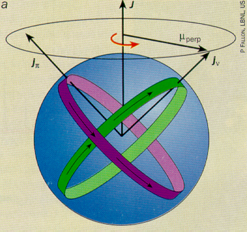
Figure 50: Magnetic rotation. The high-$j$ proton particles ($\pi$) and neutron holes ($\nu$) form current loops embedded in the near spherical mass distribution of the nucleus. These current loops as well as the associated transverse magnetic moment $\mu_{perp}$ allow one to specify the angle $\psi$ of a rotation around the axis $\vec{J}$. The total angular momentum $J$ increases by the gradual alignment of the particle and hole angular momenta $\vec{j}_{\pi}$ and $\vec{j}_{\nu}$. This is called the Shears Mechanism. The interaction due to shape polarization tries to keep $\vec{j}_{\pi}$ and $\vec{j}_{\nu}$ at a right angle, like the spring of a pair of shears. Figure from [132]

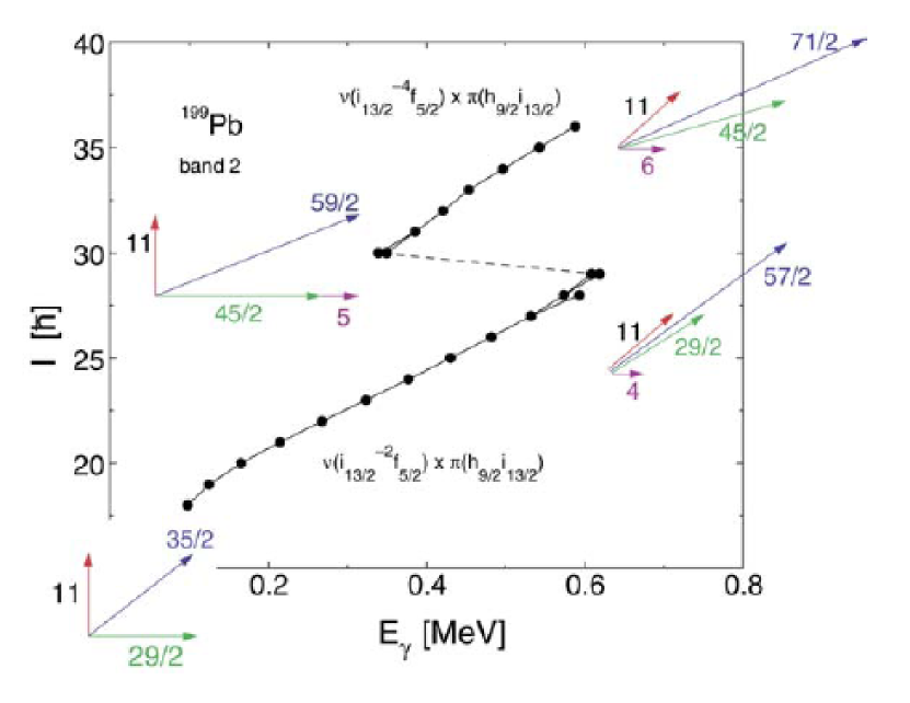
Figure 51: Angular momentum as a function of the $\Delta I=1$ transition energies $E_{\gamma}=\hbar\omega$ for band 2 in ¹⁹⁹Pb. The arrows display the following configurations: 11 red $\left[\pi(h_{9/2}i_{13/2})_{11^{-}}\right]$, 29/2 green $\left[\nu(i_{13/2}^{-2})_{12^{+}}f_{5/2})\right]$, 45/2 green $\left[\nu(i_{13/2}^{-4})_{12^{+}}f_{5/2})\right]$. No particle-hole character is indicated for the $f_{7/2}$ quasineutron. The total angular momentum $\vec{J}$ is displayed by black arrows and the core angular momentum $\vec{R}$ by purple arrows. From Ref. [134].

The angular momenta of the high-j protons and of the high-j neutron holes, which are separately lined up, are represented by the two arrows $\vec{j}_{\pi}$ and $\vec{j}_{\nu}$, respectively. Since this arrangement breaks the ${\cal R}_{z}(\psi)$ symmetry, a rotational band is the consequence, as observed. There is no ${\cal R}_{z}(\pi)$ symmetry in accordance with the observed $\Delta I=1$ sequences. The separate configurations $[\pi(h_{9/2}i_{13/2})_{11^{-}}]$ and $\left[\nu(i_{13/2}^{-2})_{12^{+}}f_{5/2})\right]$, have ${\cal R}_{z}(\psi)$ symmetry. They are well known isomeric states in the even-$N$ Pb isotopes, which are collected in Table 4. No rotational levels are found on top of these states. The dipole bands appear only when the two structures are combined including a substantial angle.

The high-$j$ orbitals have toroidal density distributions, which are illustrated by the two loops. The interaction between the particles and the holes is repulsive and favors an angle of $90^{o}$, at which the two loops are as far from each other as possible. Along the band, the total angular momentum is increased by gradually aligning $\vec{j}_{\pi}$ and $\vec{j}_{\nu}$. This process has been dubbed the ”shears mechanism” [137] because the motion resembles the closing of a pair of sheep-shears, which have a spring to keep them open. For this reason the magnetic dipole bands are also referred to as ”shears bands” [137]. Closing the blades of the shears increases the energy because the loops are aligning. If the two blades are long it takes many steps (increments of $J$ by 1$\hbar$) until the shears are closed. The energy increases gradually, resulting in the observed smooth increase of the frequency $\omega$ ($=dE/dJ$) with $J$. The function $\omega(J)$ and its derivative, the inverse of the moment of inertia ${\cal J}^{(2)}$, are determined the interaction between the high-$j$ orbitals, which will be analyzed below.

The shears arrangement of the high-$j$ orbitals gives rise to a large transverse magnetic dipole moment $\mu_{\perp}$. The protons contribute an orbital part and a spin part ($g_{p}>0$) to the magnetic moment $\vec{\mu}$, which align to $\vec{j}_{\pi}$. The spin part of the neutrons is anti-parallel to $\vec{j}_{\nu}$ ($g_{\nu}<0$). Thus all transverse components add up. It is this long transverse dipole that rotates and generates the strong magnetic radiation. As seen in Fig. 50, the rotating transverse magnetic moment decreases as the blades close, which means that the shears mechanism can be directly seen as a decrease of the $B(M1)$ values. For this type of rotation, the transverse magnetic dipole moment is a measurable quantity that specifies the orientation angle. The rotating magnetic vector generates strong $M1$ transitions between the adjacent members of the rotational band, which allows the experimentalist to arrange the transitions into a rotational sequence. In this sense it is an order parameter that indicates the coherence of the nucleonic motion. In case of ordinary rotation it is the large electric quadrupole moment that plays this role in generating the strong $E2$ transitions, which are use to identify a rotational band. The analogy suggests adopting the respective terminology ”magnetic” and ”electric” to distinguish between the two types of rotation [139], the relation of which is illustrated by Fig. 52.

Figure 52: The relation between electric and magnetic rotation. From Ref. [139].

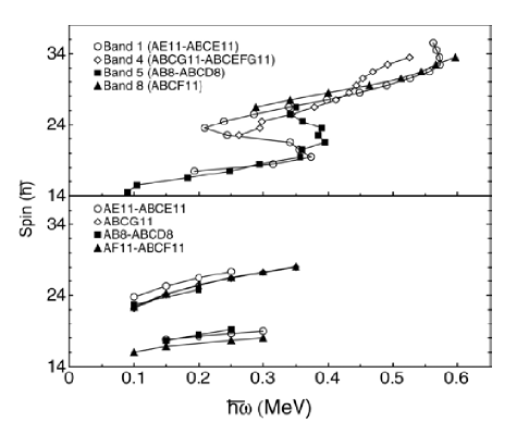
Figure 53: Left panel: Angular momentum and $BM1$ values as functions of the rotational frequency for the high-j quasiparticle configuration $[(\pi h_{9/2}i_{13/2})_{11^{-}})\times(\nu i_{13/2}^{-2})_{12^{+}}f_{5/2}]$ in ¹⁹⁹Pb (band 2). There is an additional $f_{5/2}$ quasineutron excited, which is not explicitly indicated. Full lines are the tilted axis cranking calculation. Points are the experimental data. The details of the tilted axis cranking calculations are given in Refs. [87, 137]. From Ref. [14].
Right panel: Experimental (upper panel) and calculated (lower panel) angular momentum as a function of the angular frequency of the positive parity bands in ¹⁹⁶Pb. The Cranked Shell Model letter code is used, which denotes the $i_{13/2}$ quasineutrons by A, B, C, D and the $\pi=-$ quasineutrons by E, F, G. The proton configurations $[(\pi h_{9/2}i_{13/2})_{11^{-}}]$ and $[(\pi h_{9/2}^{2})_{8^{+}}]$ are denoted by 11 and 8. The tilted axis cranking calculations are described in Ref. [138]. From Ref. [134].

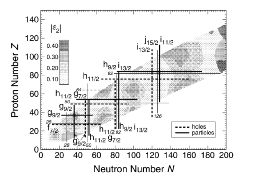
Figure 54: Schematic diagram of regions of expected magnetic rotation. Full lines indicate the location of high-j particles and dashed lines those of the high- j holes. The grey scale gives the deformation. The regions where full and dashed lines cross are particularly favored for magnetic rotation From Ref. [139].

Tilted axis cranking calculations quantitatively reproduce the salient features of the dipole bands: the nearly linear relation between frequency and angular momentum, the large values of $B(M1)$, which decrease with angular momentum, and the small values of $B(E2)$. As an example, Fig. 53 left shows the tilted axis cranking results [87, 137, 136] for the above discussed high-j configuration $[(\pi h_{9/2}i_{13/2})_{11^{-}}\times(\nu i_{13/2}^{-2})_{12^{+}}f_{5/2}]$ in ${}^{199}_{82}$Pb₁₁₇ (band 2). In the frame of the tilted axis cranking approach, the interaction between the high-j orbitals is due to the slightly oblate average potential, which is induced by them. It also ensures the alignment of the protons to one blade and of the neutron holes to the other. As discussed in the A, the high-j holes tend to align their angular momentum with the symmetry axis, whereas the high-j particles prefer the perpendicular orientation. The angle between the two blades $\vec{j}_{\pi}$ and $\vec{j}_{\nu}$ results from the balance between the inertial forces generated by $-\vec{\omega}\cdot\vec{J}$, which try to align the two vectors with the axis of rotation $\vec{J}$ and the restoring force of the slightly deformed potential, which tries to keep the two loops at $90^{o}$. The opening angle decreases with increasing $\omega$, because the inertial forces get stronger. The angular momentum vector $\vec{J}$ keeps an angle of about $45^{o}$ with the principal axes of the density distribution. It should be stressed at this point that the substantial moments of inertia of the shears bands cannot be attributed to the slight deformation. According to the tilted axis cranking calculations the shears mechanism contributes two thirds to the moment of inertia ${\cal J}^{(2)}$, whereas only one third is due to the low-j particles, which generate the slightly deformed mean field.

The right panel of Fig. 53 summarizes the functions $J(\omega)$ of magnetic dipole bands observed in ¹⁹⁶Pb. The backbends appear when the shears are closed (or almost closed). Then a pair of neutron holes is excited which extend the length of the neutron blade. The shears open again releasing some of the stress exerted by the force. Fig. 51 illustrates this in-out-in motion of the blades for band 2 in ¹⁹⁹Pb. The red arrows show the proton configuration $\left[(\pi h_{9/2}i_{13/2})_{11^{-}}\right]$. The green arrows the show the neutron configuration $\left[\nu(i_{13/2}^{-2})_{12^{+}}f_{5/2})\right]$ below the backbend and $\left[\nu(i_{13/2}^{-4})_{20^{+}}f_{5/2})\right]$ above. The left panel of Fig. 53 shows that the tilted axis cranking calculations describe the energies and $B(M1)$ values of band 2 rather well.

Magnetic rotation is expected in other regions of the nuclear chart, where high-j proton particles combine with high-j neutron holes, or vise-versa, and the nuclear deformation is small. In Fig. 54 we show our early predictions of its appearance in Ref. [139]. By now magnetic rotation has been found in all predicted regions that are experimentally accessible (see reviews [14, 140, 133, 134, 135]). The agreement between experiment and theory in Fig. 53 is typical for tilted axis cranking calculations in other regions, for which Table 3 provides examples. Meng and Zhao discuss tilted axis cranking calculations based on the relativistic mean field (RMF) approach in their contribution to this Focus Issue [42]).

The experimental indicators for magnetic rotation can be summarized as follows.

1. A $\Delta I=1$ sequence of strong magnetic dipole transitions, corresponding to $B(M1)>1\mu_{N}^{2}$,

2. A smooth increase of the $\gamma$ transition energy with angular momentum,

3. A substantial moment of inertia of ${\cal J}^{(2)}>0.2{\cal J}_{rig}$,

4. Small deformation of $\beta<0.15$,

5. Weak or absent quadrupole transitions, corresponding to $\beta_{t}<0.10$,

6. A large ratio of $B(M1)/B(E2)>10(\mu_{N}/\mathrm{eb})^{2}$,

7. A large ratio $RJB={\cal J}^{(2)}/B(E2)>100\hbar^{2}\mathrm{MeV}^{-1}(\mathrm{eb})^{-2}$ or $RJB/RJB(2^{+})>10$.

Here $RJB/RJB(2^{+})$ is given by Eq. (4).

Table 3 exemplifies the essential features of magnetic rotation from different mass regions. The transition deformations $\beta_{t}$ expresses the quadrupole transition matrix element by the liquid drop deformation parameters (1-5)

$${\cal M}_{-2}(E2)=\frac{3}{4\pi}Ze(1.2\mathrm{fm})^{2}A^{2/3}\beta_{t}.$$ (130)

The $B(E2)$ values are proportional to the square of the transition deformation parameter $\beta_{t}$. The values listed in Table 3 are consistent with the equilibrium deformations $\beta_{TAC}$ from tilted axis cranking calculations. The reduction reflects the tilt angle $\beta_{t}=\beta_{TAC}\sqrt{3/8}\sin^{2}\vartheta$. To emphasize the difference to the collective rotational mode of the Unified Model the ratio of the $RJB/RJB(2^{+})$ is added to the table (see discussion at the beginning of this section before Eq. (4)).

$A$	$Z$	$\#$	${\cal J}^{(2)}$	$\frac{{\cal J}^{(2)}}{{\cal J}_{rig}}$	$RJB$	$\frac{RJB}{RJB(2^{+})}$	$B(M1)$	$B(E2)$	$\beta_{t}$	$\frac{B(M1)}{B(E2)}$	$\beta_{TAC}$
199	82	B	22	0.23	280	48	2.0	0.078	0.029	25	-0.10a
139	62	G	12	0.23	43	5.3	1.5	0.29	0.094	5.2	0.10b
142	64	J	22	0.29	220	28	1.1	0.10	0.052	11	-0.095c
110	48	Q	13	0.37	130	11	3.8	0.10	0.083	38	0.12d
108	50	B	32	0.94	800	78	1.0	0.041	0.051	24	-0.09e
84	37	G	8.8	0.39	150	9.3	0.58	0.052	0.093	11	0.13f

Table 3: Examples of magnetic rotational bands in different mass regions. The column $\#$ quotes the label of the band in the ENSDF compilation [25]. The ratio ${\cal J}/{B(E2)}$ is denoted by $RJB$, its value for the 2${}^{+}_{1}$ state is taken from the global expression (4). Units: ${\cal J}(\hbar^{2}$ MeV^-1), $RJB(\hbar^{2}$MeV^-1 (eb)${}^{-2})$, $B(M1)(\mu^{2}_{N})$, $B(E2)$((eb)${}^{2})$. The transition deformation is given by Eq. (130). Data and tilted axis cranking calculations are taken from Refs. ^a[136, 138], ^b [141], ^c[142], ^d[143, 14], ^e [144], ^f [145].

Naturally there is a gradual transition between magnetic and electric (collective) rotation and the limits are to some extent arbitrary. One may consider which are the important transitions that constitute the rotational sequence. These are the $\Delta I=2$ electric quadrupole transitions for the electric (collective) rotation, and the $\Delta I=1$ magnetic dipole transition for magnetic rotation. The branching ratio of a decay from a given level favors M1 if

$$\frac{B(M1,I\rightarrow I-1)}{B(E2,I\rightarrow I-2)}>2.8(\hbar\omega)^{2},$$ (131)

where the units MeV, $\mu_{N}^{2}$ and (eb)² are used. With a frequency of $\sim 0.4\mathrm{MeV}/\hbar$, which is typical for the middle of the bands, the ratio should be larger than 0.5 $(\mu_{N}/\mathrm{eb})^{2}$. The ratios in Table 3 are much larger, which correspond to the strong suppression of the E2-transitions. The reason is the small deviation of the charge density from symmetry with respect to the rotational axis. The very small values of $\beta_{t}$ listed in Table 3 can be compared with the transition deformation of well deformed axial nuclei. For low-K ($<$2) bands $\vartheta\approx 90^{\circ}$ $\beta_{t}=\sqrt{3/8}\beta=0.61\times 0.3=0.18$, which corresponds to $B(E2)=1.4(\mathrm{eb})^{2}$. The gyromagnetic ratios $|g_{j}-g_{R}|$ are typically below 0.5$\mu_{N}$, which gives $\mu_{3}\sim|g_{j}-g_{R}|K<1\mu_{N}$ and $B(M1)<0.12\mu_{N}^{2}$. Putting these estimates into Eq. (131), one finds that the E2 transitions dominate for $\hbar\omega>0.170$ MeV. Accordingly, the bands have electric character, only few M1 transitions are seen near the band head, if any. The signature partners (A, B) and (E, F) in Fig. 9 are examples. High-K bands have a mixed character. The magnetic moment $\mu_{3}$ is larger and so the $B(M1)$ values. For example, the band K1 in ¹⁶³Er has a ratio $B(M1)/B(E2)\approx 1.5(\mu_{N}/\mathrm{eb})^{2}$ (see Fig. 38). The M1- transitions are seen up to $I=55/2$ for the experiment shown in Fig. 9.

4.3 Shears geometry

The simple geometry shown in Fig. 51 and the left panel of Fig. 55 opens a more phenomenological perspective taken by Macchiavelli et al. [146, 148, 147] (see also Refs. [14, 133, 134]). We discuss it, slightly generalized, for the shears band 1 in ¹⁹⁹Pb, to which the configuration $[(\pi h_{9/2}i_{13/2})_{11^{-}}\times,(\nu i_{13/2}^{-3})_{33/2^{+}}]$ is assigned. The spinning clockwork is very simple. Only two gyroscopes called the shears blades generate most of the angular momentum by gradually aligning. The two blades are composed of high-j orbitals in stretched coupling, $[(\pi h_{9/2}i_{13/2})_{11^{-}}]$ and $[(\nu i_{13/2}^{-3})_{33/2^{+}}]$. Experimentally, the band starts at $I_{h}=39/2$ and terminates at $I_{t}=59/2$. It is assumed that the band terminates when the two blades align. The angular momentum of the aligned blades is $I=55/2$. The difference is attributed to the core of the remaining 6 $pf$ neutron holes. To keep things simple and guided by the tilted axis cranking calculations it is assumed that core angular momentum $\vec{R}$ is aligned with neutron blade and proportional to $\omega$,

$$R(I)=\Theta_{R}\omega(I),~{}~{}E_{R}(I)=\omega(I)R(I)/2,~{}~{}\Theta_{R}=R_{t}/\omega_{t},$$

$$J=I+1/2,~{}~{}J_{\nu}=j_{\nu}+R(I)+1/2,~{}~{}J_{\pi}=j_{\pi}+1/2.$$ (132)

For $\hbar\omega(I)$ the experimental transition energies are taken, and $\hbar\omega_{t}=0.554$ MeV is the energy of the last transition before the termination of the band. The terms 1/2 represent the common quantal correction to the classical expressions. The geometry of the arrows in Fig. 55 (left panel) gives

$$\cos\vartheta=\frac{J^{2}-J_{\pi}^{2}-J_{\nu}^{2}}{2J_{\pi}J_{\nu}},~{}~{}\sin\vartheta_{\pi}=\sin\vartheta\frac{J_{\nu}}{J},~{}~{}\sin\vartheta_{\nu}=\sin\vartheta\frac{J_{\pi}}{J},$$ (133)

where $\vartheta$ is the angle between the blades and $\vartheta_{\pi}$ and $\vartheta_{\nu}$ the respective angles of the blades with $\vec{J}$. The value $R_{t}$ is taken such that $\vartheta=0$ at the terminating spin. For the studied configuration $j_{\pi}=11\hbar$, $j_{\nu}=16.5\hbar$ and $R_{t}=2\hbar$. The semiclassic expressions (3.1-77) can be directly applied to the shears bands. The expressions become more illustrative when re-expressing them in terms of the angles $\vartheta_{\pi}$ and $\vartheta_{\nu}$. The two separate blades are observed as isomer states in the Pb-isotopes [25]. Their static magnetic moments $\mu_{s}=\langle II|\mu_{z}|II\rangle$ and quadrupole moments $Q_{s}=\langle II|\hat{Q}_{s}|II\rangle$ are measured, which are collected in Table 4. According to Eqs. (3.1,3.1) ($\vartheta=0$) static moments are related to intrinsic moments by $\mu_{s}=\mu/(1+1/2I)$ and $Q_{s}=Q/(1+3/2I)$. Expressed in terms of $\vartheta_{\pi}$ and $\vartheta_{\nu}$, Eq. (69) becomes

$$B(M1,\,I\rightarrow I-1)=\frac{3}{8\pi}\left(\sin\vartheta_{\pi}\mu_{\pi}-\sin\vartheta_{\nu}\mu_{\nu}\right)^{2}.$$ (134)

The left panel of Fig. 56 shows that Eq. (134) reproduces well the experimental $B(M1)$ values with $\mu_{\pi}=10.5\mu_{N}$ and $\mu_{\nu}=-2.0\mu_{N}$ which correspond to $\mu_{s}=10.0\mu_{N}$ and $-1.8\mu_{N}$, respectively. Although somewhat on the low side, the adopted values are consistent with the static magnetic moments of the isomers in Table 4.

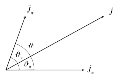
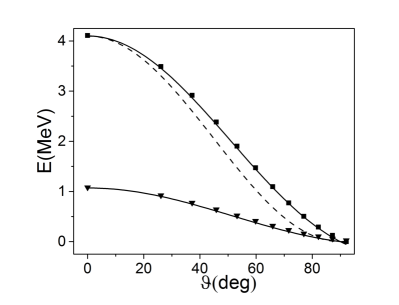
Figure 55: Left panel: Geometry of the angular momenta in a shears band. Right panel: Experimental rotational energies (squares) of the high-$j$ quasiparticle configuration $[(\pi h_{9/2}i_{13/2})_{11^{-}})\times(\nu i_{13/2}^{-2})_{12^{+}}f_{5/2}]$ in ¹⁹⁹Pb (band 2) as a function of the shears angle $\vartheta$ calculated by means of Eqs. (4.3) and (133). The squares correspond to the rotational rotational sequence in the left panel of Fig. 53. The triangles show the core rotational energy. The full curves show fits of the expression $A\cos^{2}\vartheta+B\cos\vartheta$ to the points. The dashed curve shows a fit of the expression $A\cos^{2}\vartheta$.

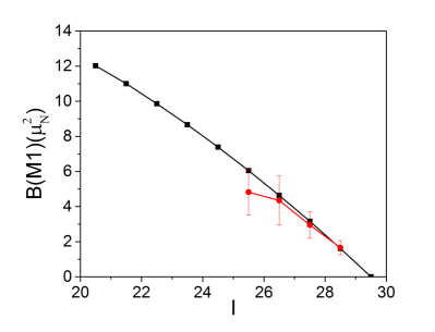
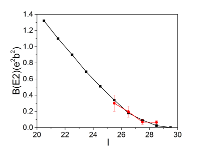
Figure 56: Reduced transition probabilities of the high-$j$ quasiparticle configuration configuration $[(\pi h_{9/2}i_{13/2})_{11^{-}}\times,(\nu i_{13/2}^{-3})_{33/2^{+}}]$ in ¹⁹⁹Pb (shears band 1) calculated by means of Eqs. (134) and (135) compared with the data from Ref. [136].

		$\left[\pi(h_{9/2}i_{13/2})_{11^{-}}\right]$			$\left[\nu(i_{13/2}^{-2})_{12^{+}}\right]$
A	$E_{x}$(MeV)	$\mu_{s}(\mu_{N})$	$Q_{s}$(eb)	$E_{x}$(MeV)	$\mu_{s}(\mu_{N})$	$Q_{s}$(eb)
192	2.743		-2.9(3)	2.624	-2.08(2)	0.32(4)
193	2.584+xa	9.9(4)a	-2.8(3)a	$x\approx 0.165^{b}$	-1.16(1)b	0.19(1)b
193				2.612+xd	-2.82(15)d	0.45(4)d
194	2.933	11.3(2)	-4.5(9)	2.628	-2.07(12)	0.48(3)
196	3.192	11.0(3)	-3.4(7)	2.694	-1.90(6)	0.65(5)
198	3.489			2.821	-1.86(2)	0.75(5)
199				2.559c	-1.076(3)c
199				3.491d	-2.39(15)d
200	3.182			3.005	-1.84(1)	0.79(3)

Table 4: Energies, static magnetic and electric quadrupole moments of Pb isotopes. The superscripts indicate configurations that deviate from the heading: a: $\left[\pi(h_{9/2}i_{13/2})_{11^{-}}\times\nu i_{13/2}^{-1}\right]$, b: $\left[\nu i_{13/2}^{-1}\right]$, c: $\left[\nu(i_{13/2}^{-2})_{12^{+}}f_{5/2})\right]$, d: $\left[\nu i_{13/2}^{-3})_{33/2^{+}}\right]$. Data from [25]. If several measurements are quoted the weighted average is given.

The $B(E2)$ values in the right panel of Fig. 56 are calculated assuming axial shape for the two blades and that the quadrupole moments of the blades add, i.e. $Q_{0}=Q_{0\pi}+Q_{0\nu}$ and $Q_{2}=Q_{2\pi}+Q_{2\nu}$. Eq. (75) can be re-written as

$$B(E2,\,I\rightarrow I-2)=\frac{15}{32\pi}\left[Q_{0\pi}\sin^{2}\vartheta_{\pi}+Q_{0\nu}\sin^{2}\vartheta_{\nu}\right]^{2}.$$ (135)

The right panel of Fig. 56 shows that Eq. (135) reproduces well the experimental $B(E2)$ values with $Q_{0\pi}=-5.0$ eb and $Q_{0\nu}=0.9$ eb, which correspond to $Q_{s\pi}=$-4.4 eb and $Q_{s\nu}$=0.8 eb. The proton values are consistent with the experimental static quadrupole moments in Table 4 ($Q_{s\pi}=$-4.5 (9) eb ($A=$194) and $Q_{s\pi}=$-3.4 (7) eb ($A=$196)). The static quadrupole moment of the $33/2^{+}$ neutron configuration is not measured but it is expected to be similar to $Q_{s\nu}\approx 0.8$ eb for the $12^{+}$ isomers in the even -$N$ neighbors (compare $A=$193 with 194).

The static magnetic and quadrupole moments of the band head $29/2^{-}$ of the shears band in ¹⁹³ Pb are measured. For the assigned configuration $\left[\pi(h_{9/2}i_{13/2})_{11^{-}}\times\nu i_{13/2}^{-1}\right]$ Eq. (133) gives $\vartheta_{\pi}=26^{\circ}$ and $\vartheta_{\nu}=47^{\circ}$ for the blade angles ($\Theta_{R}=0$ no estimate possible). Re-expressed in $\vartheta_{\pi}$ and $\vartheta_{\nu}$ Eq. (3.1) reads

$$\mu_{s}=\frac{I}{I+1/2}[\mu_{\pi}\cos\vartheta_{\pi}+\mu_{\nu}\cos\,\vartheta_{\nu}].$$ (136)

Using the values $\mu_{\pi}=12.4\mu_{N}$ and $\mu_{\nu}=-1.2\mu_{N}$ derived from the static magnetic moments of the blades in Table 4 ($A=194$ and 193), respectively) gives $\mu_{s}=9.9\mu_{N}$ for the static magnetic moment of the isomeric band head, which agrees with the experimental value $\mu_{s}=9.9(4)\mu_{N}$. Assuming that the quadrupole moments of the blades add up, Eq. (3.1) becomes

$$Q_{s}=\frac{I}{I+2/3}\Bigl{[}<Q_{0\pi}>\left((\cos\vartheta_{\pi})^{2}-{1\over 2}(\sin\,\vartheta_{\pi})^{2}\right)+$$

$$<Q_{0\nu}>\left((\cos\vartheta_{\nu})^{2}-{1\over 2}(\sin\,\vartheta_{\nu})^{2}\right)\Bigr{]}.$$ (137)

Combining the values $Q_{0\nu}$=0.23 eb ($A=$193) with $Q_{0\pi}=$-5.1 eb ($A=$194) and -3.8 eb ($A=$196) derived from the static quadrupole moments of the blades in Table 4 gives the respective the static quadrupole moments -3.1 eb and -2.4 eb for the isomeric band head, which agree with with the experimental value $Q_{s}=-2.8(3)$ eb within the experimental uncertainty.

The right panel of Fig. 55 shows the experimental rotational energy of band 2 in ¹⁹⁹Pb as a function of the shears angle $\vartheta$. In this case the blades $[(\pi h_{9/2}i_{13/2})_{11^{-}}]$ and $\left(\nu i_{13/2}^{-2})_{12^{+}}f_{5/2})_{29/2}\right)]$ have the lengths $j_{\pi}=11\hbar$ and $j_{\nu}=14.5\hbar$. In order to have $\vartheta=0$ at terminating spin 59/2 the core angular momentum is chosen $R_{t}=3.5\hbar$, which with the energy of the last transition gives $\Theta_{R}=3.5\hbar$/(0.618 MeV/$\hbar$). The major part of the rotational energy is generated by the repulsive interaction between the particles in one blade and the holes in the other. Macchiavelli et al. [146, 147, 148] suggested that this ”bladon interaction” represents the interaction between the quadrupole moment of one blade and the quadrupole moment induced by the other blade. Such effective interaction mediated by the exchange of a quadrupole phonon depends on blade angle $\vartheta$ as

$$V(\vartheta)=V_{2}D^{2}_{00}(\vartheta)=(3\cos^{2}\vartheta-1)/2.$$ (138)

The dashed line in the figure shows that the rotational energy changes roughly as $\cos^{2}\vartheta$. The strength $V_{2}$ is consistent within a factor of 2 with experimental coupling strength of quasiparticles with quadrupole vibrations in odd-A nuclei [6, 133]. The same mechanism works in tilted axis cranking description of the shears bands. The slight oblate equilibrium deformation is induced by the high-j orbitals, and the rotational energy appears as a consequence of the interaction of the high-j orbitals with the deformed potential (see the discussion in A). A detailed discussion can be found in Ref. [14].

As shown by the full line in Fig. 55, the experimental rotational energy is reproduced by the function $E(\vartheta)=4.1(0.6\cos^{2}\vartheta+0.4\cos\vartheta)$ MeV. One quarter of the total is the core rotational energy, which is not far from the ratio 1/3 found by tilted axis cranking calculations. The remaining part, the bladon interaction, is described by

$$V(\vartheta)=E(\vartheta)-E_{R}(\vartheta)=3.0(0.6\cos^{2}\vartheta+0.4\cos\vartheta)\mathrm{MeV}.$$ (139)

The curve $J(\omega)$ from the tilted axis cranking calculation for the band 2 shown in Fig. 53 can be well reproduced by $V(\vartheta)=2.3(0.43\cos^{2}\vartheta+0.57\cos\vartheta)$ MeV, which suggests that the deviations of the energy from the pure $\cos^{2}\vartheta$ shape can be attributed to additional mechanisms that are excluded from the simple phenomenological approach but taken into account in the tilted axis cranking calculations. Candidates are the interaction blades with the core, the possibility that the high-j constituents of the blades are not rigidly coupled and pairing correlations. Van Isacker and Macchiavelli [149] suggested another possibility. They derived a bladon interaction of the form $V(\vartheta)=(a+b\cos\vartheta)/\sin\vartheta$ by calculating the expectation value of a typical shears configuration composed of two high-j protons and two high-j neutron holes with short range interactions. The first term has a minimum at $\vartheta=90^{\circ}$ as expected from the overlap of the wave functions of the blades. The second term shifts the minimum to a higher angle, as the $\cos\vartheta$ term in Eq. (139).

4.4 Emergence of rotational bands

The nucleus increases its angular momentum in two different ways. One is coherent rotation of the nucleus, which results in regular rotational bands. The other is exciting quasiparticles that align their individual angular momenta in an irregular way. Figs. 10 and 11 are examples for the competition of the two modes. As discussed in section 3, the rotating mean field accounts for both on equal footing. In the present section we focus on the emergence of regular rotational sequences as a consequence of spontaneous symmetry breaking, which was already preliminary addressed in the preceding sections. To start, we realize that the quasiparticle routhian (96) derives from an effective two-body routhian that is invariant with respect to rotation about the $\vec{\omega}$ axis. Rotational invariance implies that there is a family mean field solutions that break the rotational symmetry. They are related by rotation about $\vec{\omega}$ by the angle $\psi$ and have the same energy. In the space fixed coordinate system each of these mean field states rotates uniformly about the $\vec{\omega}$ axis. This motion is associated with the angle $\psi=\omega t$ which specifies the orientation of the degenerate mean field solutions. Hence, the orientation angle $\psi$ of the mean field represents the microscopic realization of the angle variable of the collective rotor wave function of the Unified Model. When the mean field is rotated all the nucleonic orbitals (gyroscopes) are rotated by the same angle, i. e. their quantal states change in a coherent way. Such orientation angle $\psi$ and the collective wave function that lives on it exist only if the mean-field solution breaks rotational symmetry with respect to the $\vec{\omega}$ axis.

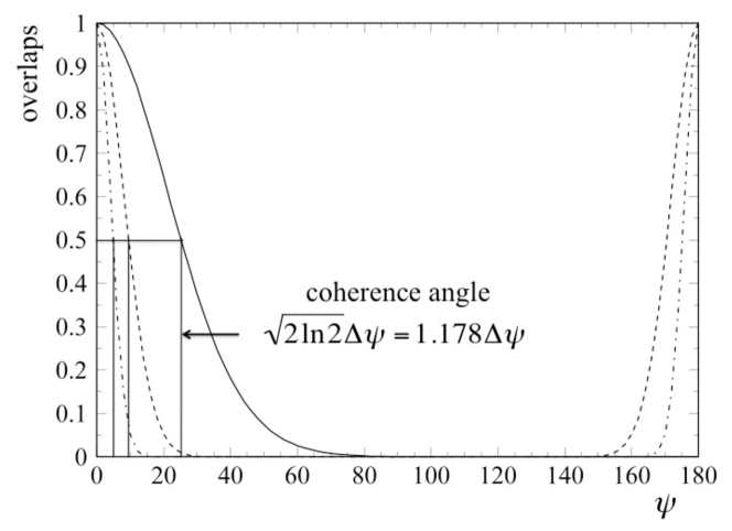
Figure 57: The overlap $|{\cal R}_{z}(\psi)|$ for a shears band (full), a normal deformed band (dash) and a superdeformed band (dash-dot). The details of the calculation are given in Tab. 5.

4.4.1 Coherence length

To quantify the degree of symmetry breaking it is instructive to introduce the notation of a ”coherence length”, which is used in other fields of many-body physics. It is the minimal length that a collective wave function can resolve. In the case of superconductivity the coherence length $\xi=\hbar v_{F}/(\pi\Delta)$ is the size of a Cooper pair . The wave function of the pair condensate cannot change more rapidly than $\xi$. When the pair condensate flows through a wire, its wave function acquires the phase $ipx/\hbar$. The phase cannot change more rapidly than $\xi$, that is $p<p_{max}=\hbar/\xi$. When the current through the wire is increased, superconductivity breaks down at the critical current density $j_{max}=e\rho p_{max}/2m=10^{3}-10^{4}A/m^{2}$.

In analogy, there exists a coherence angle $\Delta\psi$ that limits the resolution of the wave functions of collective rotation, which I call ”coherent” because the nucleons are correlated such that a common orderly motion results. The coherence angle can be determined from the overlap between the different mean field solutions $|\psi\rangle$ that specify the angle $\psi$. As illustrated by Fig. 57, the overlap between two mean field solutions rotated with respect to each other by the angle $\psi$ about $\vec{J}$ can be well approximated by a periodic Gaussian [152, 23],

$$|\langle{\cal R}_{z}(\psi)\rangle|\approx\exp\left[-\frac{\sin^{2}(\psi)}{2\Delta\psi^{2}}\right]~{}or~{}\approx\exp\left[-\frac{2}{\Delta\psi^{2}}\sin^{2}\left(\frac{\psi}{2}\right)\right],$$ (140)

where the first expression holds when there is no ${\cal R}_{z}(\pi)$ symmetry and the second when ${\cal R}_{z}(\pi)|\rangle=|\rangle$. Fig. 57 displays three examples: a superdeformed band, a normal deformed band similar to the ground band of ¹⁷⁶Hf and a shears band in ¹⁹⁹Pb (see sections 4.4.2 and 4.4.3).

The mean field state $|\rangle$ can be thought as a wave packet composed of the angular momentum eigenstates $|I,M=I\rangle$ forming the band,

$$|\rangle=\sum c_{I}|I,M=I\rangle,$$ (141)

where $I=\alpha+2n$ when ${\cal R}_{z}(\pi)$ is good. The periodic Gaussian form (140) implies a near Gaussian distribution of the coefficients

$$|c_{I}|\propto\exp\left[-\frac{(I-J+1/2)^{2}}{2\Delta J^{2}}\right],$$ (142)

which are the Fourier coefficients of the overlap function $\langle{\cal R}_{z}(\psi)\rangle$ (one-dimensional angular momentum projection). The width of the overlap $\Delta\psi$ is the inverse of the angular momentum width $\Delta J$, because

$$\Delta\psi\Delta J\approx 1$$ (143)

according to the uncertainty principle for angle and angular momentum. In this way, $|\rangle$ represents a coherent state, which is a wave packet for which the product $\Delta p\Delta x$ of the momentum and coordinate is as small as possible. It behaves as much as a classical object as permitted by the laws of quantum mechanics (see Blaizot and Ripka [24]).

The coherence angle sets the limit of how much phase $\psi I$ the rotational wave function $\exp(i\psi I)$ can acquire. That is, it restricts the number of states in the rotational band. The condition for emergence of a collective rotational wave function can be written as

$$\Delta\psi<\pi~{}~{}~{}\mathrm{if}~{}~{}~{}{\cal R}_{z}(\pi)|\rangle\not=|\rangle~{}~{}~{}\mathrm{or}~{}~{}~{}\Delta\psi<\pi/2~{}~{}~{}\mathrm{if}~{}~{}~{}{\cal R}_{z}(\pi)|\rangle=|\rangle.$$ (144)

The coherence angle must be small enough to resolve a phase increment of a half or a quarter turn, respectively, to generate two different rotational wave functions. The complementary angular momentum width $\Delta J\approx\Delta\psi^{-1}$ measures how much angular momentum can be generated from the mean field state $|\rangle$. The angular momentum width is also given by the dispersion

$$\Delta J^{2}=\langle\hat{J}_{z}^{2}\rangle-\langle\hat{J}_{z}\rangle^{2}=\sum\limits_{ph}\langle ph|\hat{J}_{z}|0\rangle^{2}.$$ (145)

The sum runs over the particle-hole or two-quasiparticle excitations, depending on the version of the mean field theory.

In order to elucidate some points, we consider a simplified model for the shears bands. We assume that the rotating mean field is composed of the $I=10$ proton state $|10,10,p\rangle$ and the $I=10$ neutron-hole state $|10,10,n\rangle$, which include the shears angle of $\vartheta$,

$$|\psi=0\rangle={\cal R}_{y}(\vartheta/2)|10,10,p\rangle\times{\cal R}_{z}(\pi){\cal R}_{y}(\vartheta/2)|10,10,n\rangle$$

$$=\sum\limits_{m}D_{10,m}^{10}(0,\vartheta/2,0)|10,m,p\rangle\sum\limits_{m^{\prime}}D_{10,m^{\prime}}^{10}(\pi,\vartheta/2,0)|10,m^{\prime},n\rangle.$$ (146)

At the band head $\vartheta=\pi/2$. The overlap and the dispersion are given by

$$\langle 0|\psi\rangle=\left[\sum\limits_{m}D_{10,m}^{*10}(0,\pi/4,0)D_{10,m}^{10}(\psi,\pi/4,0)\right]^{2},$$ (147)

$$J=\langle J_{z}\rangle=2\sum\limits_{m}D_{10,m}^{10}(0,\pi/4,0)^{2}m,$$ (148)

$$\langle J_{z}^{2}\rangle=2\sum\limits_{m}D_{10,m}^{10}(0,\pi/4,0)^{2}m^{2}.$$ (149)

Numerical evaluation of Eqs. (148,149) gives $J=14.14\approx\sqrt{2}\times 10$, as expected from geometry and $\Delta J=2.23$ for the dispersion. The overlap (147) is near-Gaussian with a Half Width at Half Maximum (HWHM) of 30.3^∘, which corresponds to $\Delta\psi=0.53$ and $\Delta J=1/\Delta\psi=2.23$ assuming genuine Gaussians. The Fourier coefficients (projection on fixed $J=m+m^{\prime}$) have a close-normal distribution centered around $J=14.5$ with a right-side HWHM of 2.5, which corresponds to $\Delta\psi=2.12$.

The band terminates at $\vartheta=0$, when the mean field state becomes the $J=20$ state. For the simple model, termination appears after an increase of angular momentum by $\Delta I\approx\pi\Delta J$. This may represent a general estimate of the band length, provided the configuration does not change such that additional angular momentum becomes available. The collective wave functions that describes the band above the band head $I=14$ oscillate on the angle interval $\lambda=2\pi/(I-14)$. At termination the mean field cannot any longer resolve the oscillations. This appears for $2\pi/(\pi\Delta J)\sim 2\Delta\psi$. That is, collective rotational states emerge only up to $\lambda\sim 2\Delta\psi$, which is about the FWHM of the Gaussian. In case the mean field conserves signature (${\cal R}_{z}(\pi)$ symmetric) the resolution is reduced by a factor of 2, i. e. to the HWHM. The discussion above estimates the angular momentum available at the band head to built the rotational sequence. Closing the shears along the band reduces the dispersion $\Delta J$, which is zero for the terminating state $I=20$. Of course it has to be like this, because the difference $I-20$ shrinks.

4.4.2 Regularity and collectivity

In the framework of the Unified Model the members of a rotational band have the same intrinsic state. A less stringent condition for a rotational band is that its intrinsic structure changes in an adiabatic way with the angular momentum. That is, the quasiparticle states gradually change with $\omega$, and the mean field stays within the same $\omega$-dependent configuration. Let us formulate the condition for similar intrinsic structure of adjacent levels in a quantitative way. Since we are interested in small changes of the wave function we may use perturbation theory for comparing the adjacent states of the band. When the frequency is incremented by $\Delta\omega$, the state $|\omega\rangle$ changes as

$$|\omega+\Delta\omega\rangle=|\omega\rangle+\Delta\omega\sum\limits_{ph}|ph\rangle\frac{\langle ph|\hat{J}_{z}|0\rangle}{e_{p}+e_{h}},$$ (150)

and the total angular momentum increases as

$$J(\omega+\Delta\omega)=J(\omega)+{\cal J}^{(2)}\Delta\omega.$$ (151)

The dynamical moment of inertia

$${\cal J}^{(2)}=dJ/d\omega=2\sum\limits_{ph}\frac{\langle ph|\hat{J}_{z}|0\rangle^{2}}{e_{p}+e_{h}}$$ (152)

measures the local increment of the angular momentum with the frequency $\omega$. The state $|\omega(I+1)\rangle$ has a structure similar to $|\omega(I)\rangle$ if it differs only by particle-hole excitations with small amplitudes

$$\alpha_{ph}=\frac{|\langle ph|\hat{J}_{z}|0\rangle|}{{\cal J}^{(2)}(e_{p}+e_{h})}\ll 1.$$ (153)

If this relation is fulfilled, ${\cal J}^{(2)}(\omega)$ will change little from $I$ to $I+1$, and the spacing $\omega$ between the levels $I$ and $I+1$ will be a smooth function of $I$.

If the more stringent condition $\Delta I\alpha_{ph}\ll 1$ holds for an interval $\Delta I\gg 1$, the band is not only regular. The relation between the spin and the level spacing will be nearly linear within the interval $\Delta I$, because the nonlinear terms of a perturbation expansion of $J(\omega)$ are of higher order in $\alpha_{ph}$. The $I(I+1)$ rule of the Unified Model follows from the assumption that the Hamiltonian is quadratic in the angular momentum, which means a linear relationship between angular momentum and frequency.

An overall measure of the structural similarity is the overlap

$$|\langle\omega(I)|\omega(I+1)\rangle|^{2}=1-D,~{}~{}D=\sum\limits_{ph}\alpha_{ph}^{2}.$$ (154)

Its deviation from one , the overlap defect $D$, should be small as compared with 1. The overlap defect is also invoked in the contribution by Nakatsukasa et al. to this Focus Issue [54].

One may quantify the degree of collectivity by counting the number of particle-hole excitations in the sums (145) and (152), which is a measure how many single particle orbitals become active in generating one or two units of angular momentum. There is the problem that the sums contain many tiny terms. In order to come up with a definite number one has to set a lower limit for the matrix element $\langle ph|\hat{J}_{z}|0\rangle^{2}$. Table 5 shows two cases. If the limit is set to 0.1, the truncated sums exhaust almost the full value.

deformation	super	normal	weak
${\cal J}^{(2)}$	97	56	14
$\Delta J$	14	7.1	2.9
$HWFM$	$5^{o}$	9o	25o
$\Delta\psi$	0.087	0.13	0.37
$1/\Delta\psi$	11.4	7.5	2.7
$\alpha_{max}$	0.003	0.01	0.15
$D$	0.005	0.03	0.05
$Q_{t}$	5.2	2.6	0.7
$\mu_{t}$	0	0	3.5
$\langle ph|\hat{J}_{z}|0\rangle^{2}>0.1$
${\cal J}^{(2)}$	96	52	11
$\Delta J$	14	6.6	2.0
$n_{ph}$	96	76	14
$\langle ph|\hat{J}_{z}|0\rangle^{2}>0.5$
${\cal J}^{(2)}$	92	44	7
$\Delta J$	14	5.6	1.5
$n_{ph}$	58	22	3
$Z$	64	72	82
$N$	88	104	117
$\varepsilon$	0.6	0.3	0.1
$\Delta_{p}$	0	0.75	0
$\Delta_{n}$	0	0.70	0.75

Table 5: Upper panel: Character of the different types of nuclear rotational bands. The listed quantities are calculated by means of tilted axis cranking at $\hbar\omega=0.3$ MeV with the parameters in the lowest panel. The coherence length $\Delta\psi$ is derived from the numerical calculations of the overlap functions shown in Fig. 57. The overlap defect $D$ is calculated for a $\Delta I=2$ transition in the case of super and normal deformation and for a $\Delta I=1$ transition in the case of weak deformation. The amplitude (153) of the strongest p-h transition is given in the line $\alpha_{max}$. Only the terms with $\langle ph|\hat{J}_{z}|0\rangle^{2}$ larger than indicated are included in the sums (145) and (152). The number of terms is given by $n_{ph}$. The moments of inertia are in units $\hbar^{2}~{}\mathrm{MeV}^{-1}$, the quadrupole moments in $eb$, the magnetic moments in $\mu_{N}$ and the pair gaps in MeV. The transition quadrupole moment $Q_{t}$ is defined by Eq. (82).

4.4.3 Three examples

Fig. 57 and Tab. 5 compare the indicators of rotational behavior for nuclei with super, normal and weak deformation. As respective examples we take tilted axis cranking calculations for the yrast bands of ¹⁵²Dy and ¹⁷⁴Hf and the shears band in ¹⁹⁹Pb discussed in section 4.2.

Superdeformation

The nuclei are very well oriented. As qualitatively discussed in section 3.8.1, they are much sharper oriented than one expects from the anisotropy of the density distribution. The superdeformed nucleus has an axis ratio of 2:1. Two density distributions with this axis ratio still have an appreciable overlap at a relative angle of 90^o, whereas the overlap of the mean field states becomes already very small at an angle of 10^o. This needle-like behavior can be attributed to the nodal structure of the incompletely filled spherical states which represents a strong element of anisotropy. The number of nodes of the wave functions determines the momentum of the particles. Hence one may say that also in the case of well and superdeformed nuclei the symmetry breaking is primarily due to the anisotropy caused by the momentum distribution of the particles at the Fermi surface. The picture of a spinning clockwork of gyroscopes (see section 3.8.1) visualizes the anisotropic momentum distribution in a schematic way.

Alternatively, one may invoke the stretch picture [93], which separates the particles into two groups, one with $j_{1}>0$ and the other with $j_{1}<0$. Each group generates a strong current pattern in the 2-3 plane, which represents the element of anisotropy. The fact that the net current in the 2-3 plane is zero is not relevant for the orientation.

The dispersion $\Delta J=14$ indicates that the superdeformed mean field supports a rotational sequence of $\Delta I\sim 40$. Very regular superdeformed bands that stretch over this interval are quite commonly observed in the $A=150$ region. The overlap defect $D=0.005$ is very small. Superdeformed nuclei come closest to the assumption $D=0$ of the Unified Model. The small value of $\alpha_{max}=0.003$ ensures that the terms in expression (150) remain small enough, such that the linear relation $J(\omega)={\cal J}\omega$ holds over an extended $\omega$ range. Indeed, the moment of inertia ${\cal J}^{(2)}$ of the lowest rotational band in superdeformed ¹⁵²Dy changes only by 10% over the observed angular momentum range of $\Delta J=38$ (see e. g. picked fence spectrum in Fig. 5 in the contribution to this Focus Issue by M. A. Riley, J. Simpson and E. S. Paul [60]). These features are in line with the large number $n_{ph}=96$ of terms in the sums (145) and (152). In order to generate one or two units of angular momentum, very many orbitals align their individual angular momentum with the rotational axis by tiny amounts. This is genuine collective rotation.

The quadrupole moment of the charge distribution with respect to the axis of rotation $Q_{t}$ is large. The rotation has electric character because it is the asymmetric charge distribution that rotates and generates the strong $E2$-radiation connecting the members of the band.

Normal deformation

The larger overlap defect $D=0.03$ and the larger value of $\alpha_{max}$ imply a shorter angular momentum interval within which function $J(\omega)$ is approximately linear. Indeed, the experimental moment of inertia ${\cal J}^{(2)}$ of the ground band of ¹⁶⁴Er increases by 10% between $I=0$ and $I=10$ (see Fig. 4). The number $n_{ph}=22$ indicates a good degree of collectivity. According to the dispersion $\Delta J=7$ the mean field supports a rotational sequence of $\Delta I\sim 20$. At $I=12$, well before the termination estimate, the ground band in even-even nuclei is crossed by the s-band, which contains two aligned high-j quasiparticles. One may consider such a band crossing as a first response to stress toward termination. Termination is observed in nuclei with $N$ around 88 at $I_{t}\approx 40$ (see Fig. 2 in the contribution to this Focus Issue by M. A. Riley, J. Simpson and E. S. Paul [60]). Before termination the rotational alignments of two i_13/2 quasineutrons and two h_11/2 quasiprotons generate $I_{qp}\approx 20$ units of angular momentum. The difference of $I_{t}-I_{qp}\approx 20$ is generated by collective rotation, which well agrees with estimate of the amount of angular momentum that can be carried by the deformed mean field.

Weak deformation

The example is the magnetic rotational band 2 in ${}^{199}_{82}$Pb₁₁₇ (band 2) with the configuration $[(\pi h_{9/2}i_{13/2})_{11^{-}}\times(\nu i_{13/2}^{-2})_{12^{+}}f_{5/2}]$. Although the value of $\Delta\psi$ is two and a half times larger than for a normal deformed nucleus, the nucleus is still sufficiently well oriented to develop quantal rotation. The $i_{13/2}$ and $h_{9/2}$ protons and two $i_{13/2}$ quasi-neutrons with hole character contribute 5.1 to $\Delta J^{2}$, the remaining 3.3 come from the low-$j$ neutrons in the $fp$ orbitals. Thus most of what is going round are the four high-$j$ orbitals, which form the current loops in Fig. 50. The value of $Q_{t}$ reflects the almost symmetric distribution of charge with respect to the axis $\vec{J}$. The rotation has magnetic character, because it is the magnetic dipole that goes round generating the observed strong $M1$ transitions which connect the members of the band.

The dispersion $\Delta J\sim 3$ suggests that mean field supports a rotational sequence of $\Delta I\sim 9$. The observed shears band 2 in ¹⁹⁹Pb extends from 35/2 to 59/2, where it terminates. The difference of $\Delta I=12$ somewhat exceeds the estimate.

The value $\alpha_{max}=$0.15 ensures the regularity of the band, but it is too large to imply a linear relation $J(\omega)$ over many transitions. The largest amplitudes $\alpha_{ph}$ belong to the four high-$j$ quasi-particles, which contribute 10$\mathrm{MeV}^{-1}$ to the total moment of inertia ${\cal J}^{(2)}$. This part of the angular momentum is generated by the shears mechanism, the energetics of which are discussed in section 4.2. The low-$j$ neutrons in the $fp$ orbitals contribute $4\mathrm{MeV}^{-1}$ to ${\cal J}^{(2)}$. Because of their small particle-hole amplitudes $\alpha_{ph}<0.02$, they add a linear contribution to $J(\omega)$.

With $n_{ph}=14$, magnetic rotation is much less collective than the rotation of the normal and superdeformed nuclei. Nevertheless, it fulfills the criteria for rotational bands and shows up as such. If the limit on $\langle ph|\hat{J}_{z}|0\rangle^{2}$ is increased to 0.5, there are only 3 terms, which come from the high-$j$ particles and holes. They account for half of ${\cal J}^{(2)}$ and $\Delta J^{2}$. This part is not very collective indeed. The other half comes from nine $fp$ neutron terms and two high-$j$ terms, which are below the limit. These numbers illustrate qualitative statement made in section 4.2 that magnetic rotation consists of the rotation of few high-$j$ current loops accompanied by some collective rotation of the core.

The examples indicate that substantial coherence does not necessarily imply strong collectivity in the above sense. Traditionally the two notations are used synonymous. The decisive criterion is a sufficiently short coherence length $\Delta\psi$ which supports the phase change of the rotational wave function. The complementary angular momentum width $\Delta J$ limits the number rotational states $\Delta I\approx 3\Delta J$ that can be generated from the mean field state before the band terminates. As already pointed out, termination is only observed under favorable circumstances. The band may be crossed by other bands. Along the band, the pairing correlations may decrease and nuclear shape may change such that $\Delta J$ increases, which postpones termination.

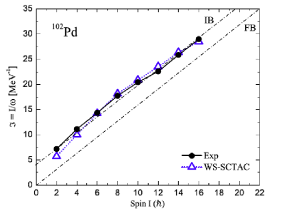
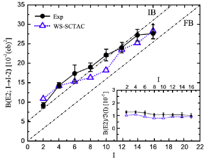
Figure 58: Left panel: Experimental moments of inertia of the ground band of ¹⁰²Pd, where $\omega=(E(I)-E(I-2))/2$ and ${\cal J}^{(1)}=I/\omega$. Right panel: Experimental $B(E2,I\rightarrow I-2)$ values of the ground band of ¹⁰²Pd. The blue lines WS-SCTAC show the calculations [154] by means of the cranked shell correction method using a Woods Saxon potential (see section 3.7). The acronym FB stands for free bosons. It denotes the limit of harmonic quadrupole oscillations described by Eqs. (4.5). The acronym IB stands for interacting bosons. It denotes a deviation from the harmonic limit that can be ascribed to a quadratic interaction between the bosons. The inset shows the ratio $B(E2,I\rightarrow I-2)/{\cal J}^{(1)}$ in units $\hbar^{-2}\mathrm{MeV(eb)}^{2}$. Taken from Ref. [15].

4.5 Tidal Waves

The Unified Model treats vibrations and rotation on equal footing assuming that they are well decoupled from the intrinsic degrees of freedom. However as illustrated by Fig. 13, the collective states near the yrast line are much less coupled to the quasiparticle background than the states of small angular momentum at the same energy. In other words, the yrast states of a vibrational multiplet are much less damped than the low-spin members. The Unified Model misses this aspect because it disregards damping. The weak damping of the vibrational yrast states allows one to describe them in the framework of the rotating mean field, which is Tidal Wave concept introduced by Frauendorf et al. [154] (and Ref. [153] with complimentary material).

Consider the phenomenological Bohr Hamiltonian (6-8) with inertial parameters $B_{\beta\beta}=B_{\gamma\gamma}=B_{i}=\sqrt{5}/2B$. Uniform rotation about the axis with the maximal moment of inertia has the lowest energy for a given angular momentum, i. e. it corresponds to the yrast states when quantized. In the co-rotating frame, the deformation parameters $\beta$ and $\gamma$ do not depend on time. Their values are given by minimizing the energy

$$E(\beta,\gamma)=\frac{J^{2}}{2{\cal J}(\beta,\gamma)}+V(\beta,\gamma),~{}~{}{\cal J}=4B\beta^{2}\sin^{2}\gamma$$ (155)

at given angular momentum $J=I\hbar$. In the case of a harmonic vibrator $V=\frac{C}{2}\beta^{2}$. Minimizing the energy one finds

$$\gamma_{e}=\frac{\pi}{2},~{}~{}~{}\beta^{2}_{e}=\frac{J}{2\sqrt{BC}},~{}~{}~{}{\cal J}=4B\beta^{2}_{e}=2J\sqrt{\frac{B}{C}},$$

$$\omega=\frac{J}{{\cal J}}=\frac{1}{2}\sqrt{\frac{C}{B}}=\frac{1}{2}\omega_{V},~{}~{}~{}E=\omega J=\omega_{V}\frac{J}{2}=C\beta^{2}_{e}.$$ (156)

The wave travels with the angular velocity $\omega$ being one half of the oscillator frequency $\omega_{V}$. The angular momentum is generated by increasing the deformation $\beta^{2}$, while the angular velocity stays constant. These are the yrast states of the vibrator multiplets described in a semiclassical way. Frauendorf et al. called the mode ”Tidal Wave” [154], because it has wave character: the energy and angular momentum increase with the wave amplitude while the frequency stays constant. Using a suitable potential one can easily incorporate unharmonicities and cover the transition to stable rotation. Bohr and Mottelson discussed the preceding in more detail in Appendix 6B-3 (Yrast Region of Harmonic Vibrations) of their Monograph [6].

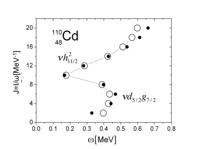
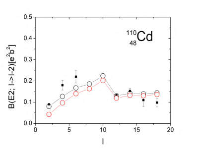
Figure 59: Left panel: Experimental moments of inertia of the ground band (black dots) of ¹¹⁰Cd, where $\omega=(E(I)-E(I-2))/2$ and $J=I$ compared with the calculations by means of the Cranking model [154] (black circles). Right panel: Experimental $B(E2,I\rightarrow I-2)$ values of ¹¹⁰Cd compared with the calculations (black circles without red circles with quantal correction, see Ref. [154]). From Ref. [15].

The yrast states of ¹⁰²Pd shown in Fig. 58 are a beautiful example of a slightly anharmonic tidal wave. Ayangeakaa et al. [155] interpreted the states as a condensate of $d$ bosons. Accordingly, up to seven bosons are observed, which align their angular momenta. If the bosons were free, the function ${\cal J}^{(1)}(I)$ would be a straight line starting at the coordinate origin (FB in Fig. 58). The experimental moment of inertia can be very well approximated by ${\cal J}^{(1)}=\Theta_{0}+\Theta_{1}I$ (IB in Fig. 58). The displacement by $\Theta_{0}$ was attributed to an interaction between the bosons that is quadratic in the boson number [156].

The inset in Fig. 58 demonstrates the wave character. The angular momentum increases solely due to the increase of the moment of inertia, which is proportional to the square of the wave amplitude $\beta_{e}$. As the $B(E2,I\rightarrow I-2)$ values are also proportional to $\beta_{e}$ the ratio is constant. The global estimate Eq. (4) gives 1.7$\times 10^{-2}\hbar^{-2}\mathrm{MeV(eb)}^{2}$, which is not far from the ratio 1.3$\times 10^{-2}\hbar^{-2}\mathrm{MeV(eb)}^{2}$ in Fig. 58.

The fact that the tidal wave is represented by a static deformation in the co-rotating frame of reference allows one to microscopically calculate its properties by means of the rotating mean field approaches. Frauendorf et al. [153, 154] calculated the energies of the yrast states and the $B(E2)$ of the intra band transitions up to spin $I=16$ for the nuclides with $Z=44-48,~{}N=65-66$. Figs. 58 and 59 exemplify the accuracy of the parameter-free calculations. In particular the change of the yrast states from the purely collective tidal wave (g-band) to the configuration with two rotational aligned h_11/2 quasiparticles (s-band) is reproduced in detail. In the case of ¹⁰²Pd (Fig. 58) the collective g-band can be followed up to $I=14$, where it is at higher energy than the s-band. This is a consequence of almost no mixing between the two configurations. In the case of ¹¹⁰Cd (Fig. 59) the collective g-band is crossed by the s-band earlier and the two bands interact stronger. The two aligned h_11/2 quasiparticles in the s-band reduce the deformation but stabilize it such that the sequence becomes more rotational. The example suggests that the method should apply to odd-$A$ and odd-odd nuclei without any further sophistication.

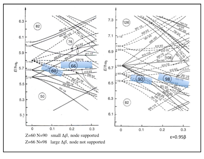
Figure 60: Energies of the modified oscillator as function of the deformation parameter $\varepsilon$. The regions of large and small coherence length are highlighted. Taken from Ref. [22].

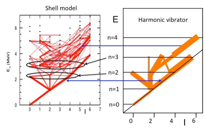
Figure 61: Left panel: Spectrum of ⁶²Ni calculated by means of the Shell Model [157]. The states are displayed as dots. The E2 transitions between the states are shown as the bars that connect the dots. The width of the bars is proportional to the $B(E2)$ value of the connecting transitions.
Right panel: Spectrum of the harmonic vibrator limit of the Bohr Hamltonian. The horizontal lines represent the multiplets of states of increasing boson number $n$. The bars indicate the E2 transition between the states, which are not explicitly marked. The width of the bars is proportional to the $B(E2)$ value of the connecting transitions.
The recognizable enhanced transitions of the Shell Model calculation are associated by means of arrows with the transitions of collective quadrupole vibrator. The ellipses enclose the regions where the two- and three-phonon multiplets are expected.

4.6 Coherence of the deformation degrees of freedom

The resolution of the collective wave function of deformation degree of freedom $\beta$ is also limited by a coherence length. It appears in the overlap of two mean-field solutions with different deformation $|\langle\beta|\beta^{\prime}\rangle|^{2}\approx\exp\left[-(\beta-\beta^{\prime})^{2}/\Delta\beta^{2}\right]$. The overlap plays a central role in describing the shape dynamics by means of the Generator Coordinate Method. Here we address it only in a qualitative way.

Fig. 60 shows the single particle levels as functions of the deformation variable $\beta$. The overlap falls off the stronger the more the occupation of the states near the Fermi surface changes over an interval of $\beta$. For $Z\approx 60$ and $N\approx 90$ many up-sloping levels cross many down-sloping. This results in a considerable re-occupation over the highlighted $\beta$ interval. A relatively small coherence length $\Delta\beta$ is expected. For $Z\approx 66$ and $N\approx 98$ there is no re-occupation within the highlighted deformation interval. The overlap will still be smaller than one, because the single particle wave functions change with $\beta$. A relatively large value $\Delta\beta$ will result. The different coherence lengths acount for the following. In the transitional nuclei around $N=90$ there is a low-lying 0${}_{2}^{+}$ state with the properties of the collective one-phonon $\beta$ vibration, but no evidence for the two-phonon state [158]. The coherence length $\Delta\beta$ is small enough to resolve one node of the vibration but too large to resolve two nodes. For the well deformed nuclei around $N=98$ there is no evidence for a collective $\beta$ vibration. The coherence length $\Delta\beta$ is too large to even resolve one node.

The left panel of Fig. 61 shows the E2 transitions obtained in a Shell Model calculation for spherical nucleus ⁶²Ni. They are compared with the transition strengths of the harmonic vibration limit of the Bohr Hamiltonian in the right panel. As discussed in section 2.4 (c. f. Fig. 13) the quadrupole vibrations become increasingly de-coherent when moving away from the yrast line. The Shell Model gives a collective 2⁺ state interpreted as the one-phonon state and at twice the energy the states 0⁺, 2⁺, 4⁺ interpreted as the two-phonon triplet. As expected for the harmonic vibrator, the transition strengths to the one-phonon state are enhanced and there are no transitions to the zero-phonon state. At variance with the harmonic oscillator, the reduced transition probability $B(E2,2^{+}_{2}\rightarrow 2^{+}_{1})$ is much smaller than the $B(E2)$ values for the $4^{+}_{1}\rightarrow 2^{+}_{1}$ and $0^{+}_{2}\rightarrow 2^{+}_{1}$ transitions, which are not twice as large as the value for the $2^{+}_{1}\rightarrow 0^{+}_{1}$ transition. The transition between the yrast states of the Shell Model are strong and may be accounted for by an anharmonic tidal wave. The Shell Model calculation moreover shows enhanced transitions parallel to the yrast sequence, which can be assisted with the yrare members of the vibrational multiplets (see Bohr and Mottelson [6], Appendix 6B-3). The remaining part of the Shell Model transition pattern looks chaotic. The coherence of the vibrational motion is lost.

5 Outlook

The Unified Model with its esthetic dichotomy of collective and intrinsic degrees of freedom represents the long wavelength limit of the collective modes compared to the granular structure of the underpinning nucleonic microstructure. The granularity becomes visible and has to be taken into account already after exciting few collective quanta. The resulting entanglement of intrinsic and rotational degrees is accounted for by the rotating mean field, which provides the possibly simplest interpretation of the multi-band structure of the yrast region. New phenomena arising from the strong coupling between the rotational and nucleonic degrees of freedom have been discovered within this framework, some of which have been discussed in this contribution. The price for the simplicity is the restriction to uniform rotation and a semiclassical description that violates angular momentum conservation. Theoretical tools beyond the mean field and the small-amplitude approximations, which combine the Generator Coordinate Method with configuration mixing (see e.g. the contributions to this Focus Issue by Egido [41], Sun [56], Walker and Xu [57], Sheikh et al. [58] and the review by Bender et al. [38]), remove these restrictions at the price of increasing the complexity of the description and drastically the computational effort. This type of calculations may describe the experimental data and allow for reliable predictions. In my view it seems important developing methods that reveal the underlying simple structures, which may be the ones discussed in this contribution or others that have not been covered (e. g. dynamical symmetries) or not anticipated yet. Particularly challenging is the question how to address the regions where the coherence of the nucleonic motion sets in or disappears. One example is the damping of rotation in ”warm nuclei” few MeV above yrast, which is discussed in the contribution to this Focus Issue by S. Leoni and A. Lopez-Martin [61]. Conceptually, one has to give up on describing the properties of individual quantum states. The rapid increase of the level density makes such predictions impossible because the results become exceedingly sensitive to the details of the Hamiltonian and to the solution scheme of the many-body problem. Part of the theoretical results must be considered as ”random”. The challenge is to decide what should be classified as random fluctuations and what as average properties described by the theory. On the other hand, allowing for a degree of randomness favors alternative many-body approaches based on sampling techniques, which open new avenues.

Acknowledgments I was lucky to come to the Niels Bohr Institute early in my scientific career. These were the hay-days of highspin physics. Copenhagen/Lund was a powerhouse of this new exciting direction, which has fascinated me until now. I became acquainted with a new style of doing theoretical work: Discuss with the experimentalists their latest results and expose your ideas to their scrutiny. These were the NBI Mondays, when the Risø group came to meet with Aage and Ben and us other theoreticians. For me these meetings were a great source of inspiration and the origin of lasting friendships. Aage and Ben had an ingenious way seeing the simple principles behind complex observations or computational results. Searching for them has become the goal of my own work. Working with these two great minds and the other outstanding scientists I met at the NBI was such a privilege. THANK YOU!
Support by the DoE grant DE-FG02-95-ER40934 is acknowledged.

6 References

Appendix A Semiclassical analysis of high-j quasiparticle states in a triaxial quadrupole potential rotating about an axis in one of its principal planes

The appendix extends the discussion of the geometry and rotational response of high-j quasiparticle orbitals in section 3.5. It is based on the work published in Refs. [65, 66, 67, 68, 69], which is supplemented by unpublished material.

The coupling of the high-j intruder state with the remaining states of the major shell to which it belongs is disregarded. This makes the quantum system one dimensional: The number of radial knots is zero, i. e. the particle moves on an orbit of fixed radius and the particle motion is restricted to the sphere of constant angular momentum,

$$j^{2}=j_{1}^{2}+j_{2}^{2}+j_{3}^{2}=j(j+1).$$ (157)

Working out the semiclassical theory it is useful to introduce the canonical operators momentum $p$ and position $q$ (canonical variables in the classical mechanics), which obey the standard commutation relation $[p,q]=-i$. One may take the angular momentum projection $\hat{j}_{3}$ as the momentum operator $q$. Then the angle operator $\hat{\phi}$ which fixes the orientation of the angular momentum vector $\vec{j}$ with respect to the 3-axis becomes the conjugate position operator $q$ and

$$[p,q]=[\hat{j}_{3},\hat{\phi}]=-i.$$ (158)

As the momentum takes only the $2j+1$ discrete values $k=-j$, …,$j$, the angle can also take only take $2j+1$ discrete values on the unit circle. These are the eigenvalues of $\hat{\phi}$, which can be chosen as

$$\phi_{n}=\frac{2\pi}{2j+1}n,~{}~{}~{}n=-j,~{},-j+1,~{}....,~{}j-1,~{}j.$$ (159)

It is common to use the momentum eigenstates $|k\rangle$ as a basis, which are related to the angle eigenstates $|n\rangle$ by the transformation

$$|k\rangle=\frac{1}{\sqrt{2j+1}}\sum\limits_{n=-j}^{j}e^{ik\frac{2\pi}{2j+1}n}|n\rangle,~{}~{}~{}|n\rangle=\frac{1}{\sqrt{2j+1}}\sum\limits_{n=-j}^{j}e^{-i\frac{2\pi}{2j+1}nk}|k\rangle.$$ (160)

The amplitude

$$\langle n|k\rangle=\frac{1}{\sqrt{2j+1}}e^{ik\frac{2\pi}{(2j+1)}n}=\frac{1}{\sqrt{2j+1}}e^{ik\phi_{n}}$$ (161)

is the discrete version of the well known expression $1/\sqrt{2\pi}\exp{[ik\varphi]}$ for the $\hat{j}_{3}$ eigenfunctions in the full orientation space. The discreteness of $j_{3}$ and $\phi$ should be kept in mind in the semiclassical analysis below.

In discrete space it is convenient to work with the operator $\exp[i\hat{\phi}]$ instead of $\hat{\phi}$ itself. Its matrix elements in the $k$ basis are

$$\langle k|e^{i\hat{\phi}}|k^{\prime}\rangle=\delta_{k,k+1},$$ (162)

which is seen using Eqs. (160) and noticing their orthonormality. Then the matrix of the operator

$$\langle k|\sqrt{j-\hat{j}_{3}}e^{i\hat{\phi}}\sqrt{j+\hat{j}_{3}}|k^{\prime}\rangle=\sqrt{(j-k)(j+k+1)}\delta_{k,k+1}$$ (163)

is recognized as the matrix of the standard $\hat{j}_{+}$ operator. Thus the operators $\hat{j}_{\pm}$ can be exposed as

$$\hat{j}_{+}=\sqrt{j-\hat{j}_{3}}e^{i\hat{\phi}}\sqrt{j+\hat{j}_{3}},~{}~{}~{}\hat{j}_{-}=(\hat{j}_{+})^{\dagger}=\sqrt{j+\hat{j}_{3}}e^{-i\hat{\phi}}\sqrt{j-\hat{j}_{3}}.$$ (164)

The standard commotion relations $[\hat{j}_{3},\hat{j}_{\pm}]=\pm\hat{j}_{\pm}$ and $[\hat{j}_{+},\hat{j}_{-}]=2\hat{j}_{3}$ are fulfilled because the matrices agree with the ones of the three operators within a set of states $|j,k\rangle$. They can also be directly verified using $\left[\hat{j}_{3},\exp[\pm i\hat{\phi}]\right]=\pm\exp[\pm i\hat{\phi}]$.

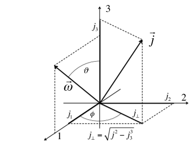
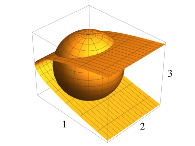
Figure 62: Left: Geometrical relation between the three Cartesian angular momentum components $j_{1},~{}j_{2},~{}j_{3}$ of the i_13/2 particle and the angle $\phi$, which is taken as the momentum conjugate to $j_{3}$. In addition the orientation of angular velocity vector $\vec{\omega}$ is shown, which is chosen to lie in the 1-3 -plane.
Right: Classical orbits of the angular momentum vector $\vec{j}$ of an i_13/2 particle in an axial potential that rotates about the 1-axis. The orbits are the line of intersection between the sphere of constant length $j$ and the parabolic cylinder of constant routhian (energy in the rotating frame). They represent two of the orbits in the lower left panel of Fig. 63, which shows the projection of the three-dimensional orbits onto the 1-3-plane.

In semiclassical approximation $\hat{\vec{j}}$ is considered as a classical vector. The commutators are replaced by the Poisson brackets. The classically corresponding momentum $j_{3}$ and position $\phi$ are canonical variables, which commute. The classically corresponding expressions for $j_{+}$ and $j_{-}$, given by Eqs. (164), can be rearranged to

$$j_{1}=j_{\bot}\cos\phi,~{}~{}j_{2}=j_{\bot}\sin\phi,~{}~{}j_{\bot}=\sqrt{j^{2}-j_{3}^{2}}.$$ (165)

A first correction to the classical expressions is obtained replacing $j^{2}$ by $j(j+1)$. We introduce the following convention. Instead of $\sqrt{j(j+1)}\approx j+1/2$ we simply use $j$. It is understood that evaluating the expressions one has to use $j+1/2$ instead of $j$, e. g. $j=7$ for an i_13/2 particle.

Quantization is realized by the Bohr-Sommerfeld rules

$$\oint pdq=\oint\phi\left(j_{3}\right)dj_{3}=S=2\pi n,$$ (166)

$$\oint qdp=\oint j_{3}(\phi)d\phi=S=2\pi n,$$ (167)

$$\int\int dpdq=\int\int d\phi dj_{3}=S=2\pi n.$$ (168)

Geometrically this means the following. The phase space is the projection of the surface of the angular momentum sphere on the cylinder with the radius $j$ and $-j\leq j_{3}\leq j$. The area between two quantized orbits is $2\pi$.

The energy in the deformed potential is determined by the orientation of $\vec{j}$ with respect to the principal axes, which can be expressed in terms of the components of the angular momentum. The expression can be derived from Eqs. (63,64) by the consideration that the quadrupole operator is constructed by coupling the two vectors $\vec{x}$ to a spherical tensor operator of rank 2. Coupling the two angular momentum vectors in the same way $\vec{j}$ results in a spherical tensor operator of rank 2, which transforms under rotation like the quadrupole tensor. As the energy of the high-j orbital depends only on its orientation with respect to the potential, it must depend on the components of $\vec{j}$ in the same way as given by Eqs. (63,64). Using the explicit expressions for the quadrupole moments in terms of the components of $\vec{x}$, one obtains

$$e^{\prime}=e-\omega(\sin\vartheta j_{1}+\cos\vartheta j_{3}),~{}~{}e=\kappa\left[\left(3j_{3}^{2}-j^{2}\right)\cos\gamma-\sqrt{3}\left(j_{1}^{2}-j_{2}^{2}\right)\sin\gamma\right].$$ (169)

For the following examples the parameter $\kappa$ is determined from the distance between the i_13/2 Nilsson levels at the deformation $\varepsilon=0.26$, which gives $\kappa=0.0086\omega_{0}$. The energies of the orbits are taken as $e^{\prime}=e^{\prime}(\omega)$ from the quantal routhians shown in the upper panels of the figures to be discussed. As discussed in context of Table 2, one can make any two of the three principal axes to be the 1- and 3-axes by choosing the appropriate $\gamma$-sector. In the following we consider only a planar tilt of the rotational axis into the 1-3- principal plane. Quantization is achieved by diagonalizing the Hamiltonian $h^{\prime}=e^{\prime}$ given by Eq. (169) within the basis of angular momentum eigenfunctions $|j,m\rangle$. The eigenvalues are called ”quantal routhians” in the following.

The orbits are determined by angular momentum and energy conservation. Without pairing, they are given by the intersection of the angular momentum sphere (157) and the energy ellipsoid (169). The time derivatives of the momentum and coordinate are given by

$$\dot{p}=v_{3}=-\frac{\partial e^{\prime}\left(j_{3},\phi\right)}{\partial\phi}=4\kappa\sqrt{3}\sin\gamma j_{2}\left(j_{1}-j_{1c}\right),$$ (170)

$$\dot{q}=\dot{\phi}=\frac{\partial e^{\prime}\left(j_{3},\phi\right)}{\partial j_{3}}$$

$$=4\kappa\sqrt{3}\left[\cos(\gamma+30^{\circ})(j_{3}-j_{3c})+\sin\gamma\frac{j_{3}j_{1}\left(j_{1}-j_{1c}\right)}{j^{2}-j_{3}^{2}}\right],$$ (171)

$$j_{1c}=-\frac{\omega\sin\vartheta}{4\kappa\sqrt{3}\sin\gamma},~{}~{}j_{3c}=\frac{\omega\cos\vartheta}{4\kappa\sqrt{3}\cos(\gamma+30^{\circ})}.$$ (172)

The stationary points of the classical motion are located at $\dot{q}=\dot{p}=0$. Minima and maxima are singular points of no motion. Any saddle point S is localized on a special orbit called separatrix, which will be labelled by S. A particle moving on a separatrix will reach the saddle point only after infinite time because velocity and acceleration go to zero. As a consequence the expectation value of $\vec{j}$ is given by the value at the saddle point.

If the stationary point is located outside the 1-3 plane, i.e. $j_{2}\not=0$, Eqs. (170,171) imply that its coordinates are $j_{1}=j_{1c},~{}j_{2}=\pm\sqrt{j^{2}-j_{1c}^{2}-j_{3c}^{2}},~{}j_{3}=j_{3c}$. If it is located in the 1-3- plane its coordinates are $j_{1}=j_{1}(\alpha_{0}),~{}j_{2}=0,~{}j_{3}=j_{3}(\alpha_{0})$, where $\alpha_{0}$ is the solution of $\dot{p}(\alpha)=0$ with $j_{1}(\alpha)=j\sin\alpha,~{}j_{3}(\alpha)=j\cos\alpha$ in Eq.(171). Except for certain simple cases, it is best finding the solution numerically.

The classical probability for the particle to be within the interval $(j_{3},~{}j_{3}+dj_{3})$ is

$$dP(j_{3})=\frac{dt}{T}=\frac{1}{|v_{3}T|}dj_{3}=\frac{1}{|4\kappa\sqrt{3}\sin\gamma j_{2}\left(j_{1}-j_{1c}\right)T|}dj_{3},$$ (173)

where $T$ is the period of the orbit. The major contributions to expectation values of physical quantities come from regions where $v_{3}$ is small. The classical probability for the particle to be within the interval $(j_{1},~{}j_{1}+dj_{1})$ is

$$dP(j_{1})=\frac{1}{|v_{1}T|}dj_{1}=\frac{1}{|v_{3}T|}\left|\frac{dj_{3}}{dj_{1}}\right|_{e^{\prime}}dj_{1}$$

$$=\frac{1}{|4\kappa\sqrt{3}\cos(\gamma+30^{\circ})j_{2}\left(j_{3}-j_{3c}\right)T|}dj_{1}.$$ (174)

In the following the projections of the orbits onto the 1-3 plane will be shown. They are given by eliminating $j_{2}$ from $e^{\prime}$ in Eq. (169) by means of Eq. (157). The resulting expression for $\gamma\not=0,\pi$ is

$$e^{\prime}=2\kappa\sqrt{3}\left[\cos(\gamma+30^{\circ})(j_{3}-j_{3c})^{2}-\sin\gamma\left(j_{1}-j_{1c}\right)^{2}\right]$$

$$-2\kappa\sin(\gamma-30^{\circ})j^{2}+\frac{\omega^{2}\sin^{2}\vartheta}{4\kappa\sqrt{3}\sin\gamma}+\frac{\omega^{2}\cos^{2}\vartheta}{4\kappa\sqrt{3}\cos(\gamma+30^{\circ})}.$$ (175)

The curves of constant energy are ellipses or hyperbolas centered at $j_{1c},~{}j_{3c}$. The axial case is treated by taking the limit $\gamma\rightarrow 0$, which gives parabolas centered at the $j_{3c}$- axis.

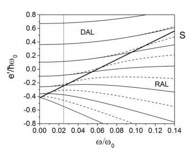
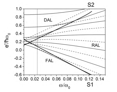
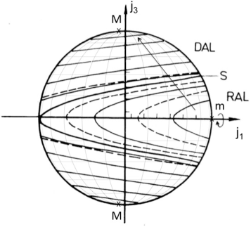
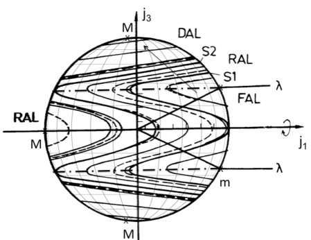
Figure 63: Routhians and classical orbits of an i_13/2 quasiparticle in the potential with $\varepsilon=0.26,\gamma=0$, rotating with the frequency $\omega$ about the 1-axis perpendicular to the symmetry 3-axis.
Upper left panel: Quantal routhians for zero pairing. The thick curve shows the energy of the separatrix S. At $\omega=0$, the levels with increasing energy have the angular momentum projection on the symmetry axis $|j_{3}|=\Omega=$1/2, 3/2, 5/2, …. . The full and dashed lines correspond to signature $\alpha=$1/2 and -1/2, respectively.
Upper right panel: Quantal routhians for $\Delta=0.12~{}\hbar\omega_{0}$ and $\lambda$ between the 3/2 and 5/2 levels. The thick lines show the energies of the two separatrices S1 and S1 in the low-right panel.
Lower left panel: Classical orbits in angular momentum space for zero pairing. The figure shows the 1-3-projection of the orbits, which lie on the surface of the sphere of fixed angular momentum. The frequency $\omega=0.025\omega_{0}$ which is indicated by the thin line in the upper panels. The energy of the orbits is the energy of the levels in the upper panels at the thin line. The energy of the orbits increases in direction of the arrows. The points of lowest possible energy are labelled with m and the point of highest possible energy with M. In order to emphasize the location of the orbits on the angular momentum sphere the lines of constant altitude and latitude are shown.
Lower right panel: Analogous to the lower left panel for finite pairing. The dash-dotted line is the orbit with $e^{\prime}(0)=\lambda$.

A.1 Axial shape, rotation about the short axis

The left panels of Fig. 63 illustrate an i_13/2 particle in the prolate potential, which rotates about the 1-axis perpendicular to the symmetry axis 3 ($\vartheta=90^{\circ},~{}j_{3c}=0$). For $\gamma=0$ the equi-energy ellipsoids become parabolic cylinders, which move to the left with increasing energy. The orbits lie at the intersection curves between the energy cylinders and the angular momentum sphere (see Fig. 62). The orbits displayed in the lower left panel have the energies of the quantal levels at $\omega=0.025\omega_{0}$ in the upper left panel.

As seen, there are two topologically different kinds of orbits, which are separated by the separatrix S. The separatrix lies at the intersection of the angular momentum sphere with the parabolic cylinder whose vertex line is tangent to the sphere. The touching point lies at $j_{1}=-j,~{}j_{2}=0,~{}j_{3}=0$. It specifies the saddle point S, as seen by putting it into Eqs. (170,171). Since it contains the saddle point, the expectation value $\langle j_{1}\rangle=-j$ for the separatrix S. The curvature of the parabolas is $6\kappa/\omega$. For $\omega\rightarrow 0$ the parabolas become horizontal lines and all lie outside S (which becomes the $j_{3}=0$ line). The orbits revolve the symmetry axis 3. This motion is caused by the torque excerted by the deformed potential and is of the same type as the precession of a top in the gravitational field. Since the precession cone is aligned with the deformation axis this type of motion is called Deformation ALigned (DAL). For each DAL state $j_{3}>0$ there is a degenerate one with $j_{3}<0$. Combining them to even and odd superpositions results in the characteristic signature doublets. For $\omega\rightarrow\infty$ the parabolas become vertical lines, which corresponds to negligible torque of the deformed potential compared to torque by the inertial forces. The vector $\vec{j}$ revolves the the 1-axis, which is the rotation axis. Accordingly, this type of motion is called Rotational ALigned (RAL). As in any symmetric potential, where even and odd states alternate, consecutive RAL states correspond to opposite signature. For intermediate values of $\omega$ the topology of the orbits is either RAL or DAL.

The upper left panel of Fig. 63 illustrates how the separatrix divides the spectrum into the DAL region above S and the RAL region below S. The separatrix is a straight line with the slope -$\langle j_{1}\rangle=j$. The fingerprints of the two coupling schemes are easily recognized. More details of the routhian diagram can be related to the classical orbits. The axis of the DAL precession cones is somewhat tilted toward $j_{1}<0$. It pierces the angular momentum sphere at the point M, which is maximum of the energy. M lies at $j_{1}=-\omega/(6\kappa),~{}j_{2}=0,~{}j_{3}=\pm\sqrt{j^{2}-\left(\omega/6\kappa\right)^{2}}$ (c. f. Eqs. (170,171).) As the consequence, the average of the $j_{1}$ value of the DAL orbits is slightly negative, which is reflected by the positive slope of the quantal routhians, which increases with $\omega$. For the RAL orbits the average value of $j_{1}$ can be estimated by means of expression (173). The right turning points contribute most because $j_{2}\rightarrow 0$. For the lowest RAL orbits the left turning point of $j_{1}$ at the vertex contributes less because $j_{2}$ is finite, and the average of $j_{1}$ is somewhat less than the values at the right turning points. When approaching S for the higher orbits, the left turning point becomes more important because $j_{2}$ decreases. That is, the average $j_{1}$ becomes more negative. For S it reaches $-j$ because the turning point becomes a stationary point. Near the separatrix quantum effects become important, which smoothly connect the DAL and RAL routhians through S. They can be interpreted as tunneling through the classically forbidden regions. For example, some signature splitting between the DAL doublets emerges, when the upper and lower orbit come close at the left turning point.

With increasing frequency the parabolas become flatter and flatter, their curvature being $6\kappa/\omega$. This means that the RAL part of the phase space increases at the expense of the DAL part. This is illustrated by the left panel of Fig. 64, which show how the separatrix changes with $\omega$. The separatrix disappears for $\omega>6\kappa/j$ when the curvature of the parabola exceeds the one of the circle. Only RAL orbits remain. The separatrix $\omega=0.3\omega_{0}$ comes close to this limit.

Fig. 21 sketches the two coupling schemes: The fingerprint for RAL coupling is a well-split sequence of states of alternating signature with approximately constant aligned angular momentum $i=\langle j_{1}\rangle=-de^{\prime}/d\omega$, which decreases with energy. The fingerprint of DAL coupling are signature doublets and small negative aligned angular momentum.

The geometry of the orbits in the presence of pairing is obtained by replacing the energy of the particle in the deformed field by its quasiparticle energy,

$$j_{1}^{2}+j_{2}^{2}+j_{3}^{2}=j^{2},~{}~{}~{}e^{\prime}=\sqrt{(e-\lambda)^{2}+\Delta^{2}}-\omega j_{1}.$$ (176)

This corresponds to introducing non-rotating quasiparticles exposed to the cranking term. Loosely speaking, it amounts to leave away the negative-energy states in Fig. 17 and their interactions with the positive-energy states. The Bogoljubov transformation is carried out for the non-rotation frame, and the equations of motion (52) are solved in the subspace of the positive-energy quasiparticles. The quantal routhians in the upper right panel of Fig 63 are obtained using this approximation.The same holds for the following examples that take pairing into account.

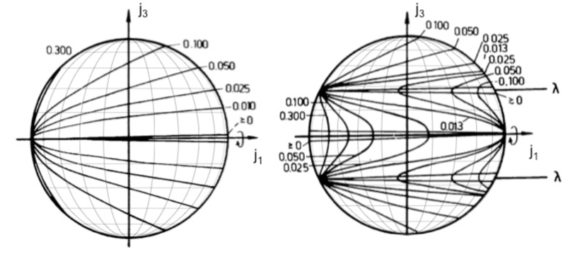
Figure 64: Sequence of separatices in Fig. 63. The separatrices are labeled by $\omega/\omega_{0}$.

The right panels of Fig 63 illustrate the case of an i_13/2 quasiparticle in the axial potential. The gap parameter is $\Delta=0.12\omega_{0}$, and $\lambda$ lies between the $\Omega=3/2$ and 5/2 levels. The dash-dotted line shows the projection of the orbit $e=e^{\prime}(\omega=0)=\lambda$. Well above it, the quasiparticle orbit becomes the particle orbit and well below the hole orbit. The latter is obtained by reflecting the particle orbit on the 2-3 plane, $j_{1}\rightarrow-j_{1}$, which can be seen by taking the limit $\Delta\rightarrow 0$ of Eq. (176). The particle-like branch is smoothly connected with the hole-like branch for finite $\Delta$. The resulting energy surfaces are fourth order cylinders with three vertices, which move from the right to the left with increasing $e^{\prime}$. The orbits are the intersection curves of the cylinders with the angular momentum sphere.

The resulting topology is more complex. A new type of orbits appears, which revolve the axis $\vec{j}_{\lambda}$ marked by $\lambda$. Frauendorf and Sobeslavsky [66, 67, 69] called it Fermi axis, because its direction is determined by $\lambda$, which is close to the Fermi level of the unpaired system. They called the orbits that revolve the Fermi axis Fermi ALigned (FAL). The FAL orbits have a finite angular momentum projection on both the 3- and 1-axes. Like for the DAL orbits there two distinct degenerate FAL orbits with $j_{3}\approx\pm j_{3\lambda}$. In contrast to the DAL orbits they have a positive value of $j_{1}\approx j_{1\lambda}$, because of the tilt of the Fermi axis. When the quasiparticle revolves the Fermi axis it changes from a particle into a hole. The quasiparticle partially decouples from the deformed potential, because the particle and hole quadrupole moments have opposite sign and tend to compensate each other. In summary, the FAL orbits have finite angular momentum components along the rotation axis 1 and the deformation (symmetry) axis 3. They appear in signature doublets, which may be slightly split by tunneling.

The FAL orbits are separated by the separatrix S1 from the RAL region, which is separated by the separatrix S2 from the DAL regions. The separatrix S2 divides the RAL region into the left part, which contains hole-like quasiparticles that anti-align with the rotational axis, and the right part, which contains particle-like quasiparticles that align with the rotational axis. As seen in the right panel of Fig. 64, the FAL region only exists for low $\omega$ and $\lambda$ about in the middle of the shell. The two separatrices divide the spectrum into the three regions, which are easily recognized in the upper right panel of Fig. 63 by their fingerprints. The crossing of S1 and S2 corresponds to the single separatrix $\omega=0.013\omega_{0}$ in the right panel of Fig. 64. For smaller frequency $\omega$ a different topology appears, which is indicated by the separatrices labeled by $\omega>0$. S1 divides the FAL region from particle-like DAL above and hole like DAL below. S2 divides the hole-like RAL interior region from the hole-like DAL regions above and below. The right panel of Fig. 64 shows how the separatrices change with $\omega$, delineating the phase spaces of the three coupling schemes.

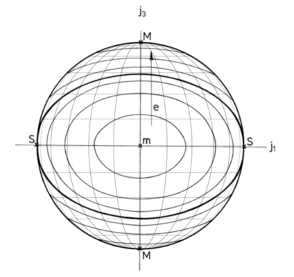
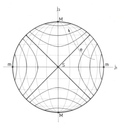
Figure 65: Classical orbits in angular momentum space for zero pairing and $\omega=0$. Left: Medium-long projection of the orbits ($\gamma=-30^{o}$), which lie on the surface of the sphere of fixed angular momentum. Right: Short-long projection of the orbits ($\gamma=30^{o}$). The minima and maxima of the energy are labeled by m and M, respectively. The energy of the orbits increases in direction of the arrow.

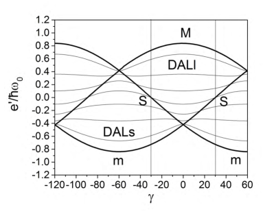
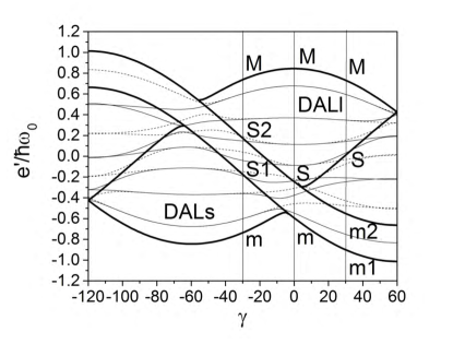
Figure 66: Left: Quantal energies of an i_13/2 quasiparticle particle in the triaxial potential with $\varepsilon=0.26$ as function of the triaxiality parameter $\gamma$ for $\omega=0$. Right: Like the left panel $\omega=0.025\omega_{0}$. The cases $\gamma=-30^{\circ},~{}0^{\circ},~{}30^{\circ}$ discussed below are indicated by vertical lines. The separatrices and the maxima and minima of the classical energy are shown as thick curves and labeled in accordance with the other figures.

A.2 Triaxial shape, rotation about a principal axis

The orbits are the intersection curves between the angular momentum sphere and the triaxial energy ellipsoid. Figs. 65 illustrate the topology of the orbits at $\omega=0$, without pairing and $\gamma=\pm 30^{o}$. In contrast to the axial potential, there are two classes of DAL orbits, the phase spaces of which are delineated by the separatrix S. The orbits $e>e_{S}$ are aligned with (precess around) the long (l-) axis. They appear where the energy ellipsoid sticks out of the angular momentum sphere. The $e<e_{S}$ orbits are aligned with the short (s-) axis. They appear where the angular momentum sphere sticks out of the energy ellipsoid. The projections onto the 1-3-plane are ellipses and hyperbolas, for $\gamma=-30^{\circ}$ and $30^{\circ}$, respectively. The separatrix corresponds to the ellipse that touches the angular momentum sphere or to the asymptotes of the hyperbolas, respectively. The ratio

$$\frac{a_{1}}{a_{3}}=\left[\frac{\sin\gamma}{\cos\left(\gamma+30^{\circ}\right)}\right]^{1/2}$$ (177)

is the ratio of the half-axes of the ellipses for $-60^{\circ}\leq\gamma\leq 0^{\circ}$ or the slope of the asymptotes for $0^{\circ}\leq\gamma\leq 60^{\circ}$. The left panel of Fig. 66 shows how the topology changes with the shape. For decreasing $|\gamma|$ the phase space of the DAL orbits aligned with the l-axis (DALl) increases at expense of the phase space of the DAL orbits aligned with the s-axis (DALs) and vice versa for increasing $|\gamma|$. For the axial limits the separatrix disappears and the orbits are circular in the medium-long projection (used in the left panel of Fig. 65). There are only DALl orbits for $\gamma=0^{\circ}$, which are horizontal lines in the short-long projection (used in the right panel of Fig. 65). There are only DALs orbits for $|\gamma|=60^{\circ}$, which are vertical lines in the short-long projection The lowest quantal routhians are shifted above the classical minima by the zero-point energy, which is larger at strong triaxility, where the orbits are well confined by the potential, than at axial shape, where they are more delocalized.

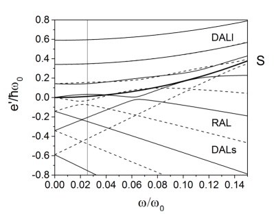
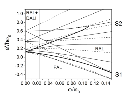
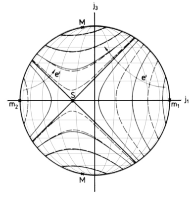
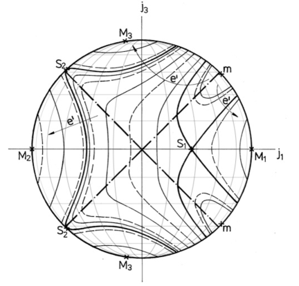
Figure 67: Routhians and classical orbits of an i_13/2 quasiparticle in the triaxial potential with $\varepsilon=0.26,\gamma=30^{\circ}$, rotating with the frequency $\omega$ about the 1- axis, which is the short axis. The layout is analog to Fig. 63.
Upper left panel: Quantal routhians for zero pairing.
Upper right panel: Quantal routhians for $\Delta=0.12~{}\hbar\omega_{0}$ and $\lambda=0$.
Lower left panel: Classical orbits in angular momentum space for zero pairing. The figure shows the 1 (short)-3 (long) -projection of the orbits, which lie on the surface of the sphere of fixed angular momentum. The frequency $\omega=0.025\omega_{0}$. The energy of the orbits increases in direction of the arrow.
Lower right panel: Analogous to the lower left panel for finite pairing. The dash-dotted line is the orbit with $e^{\prime}(0)=\lambda=0$.

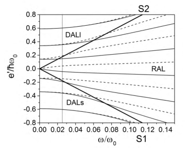
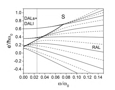
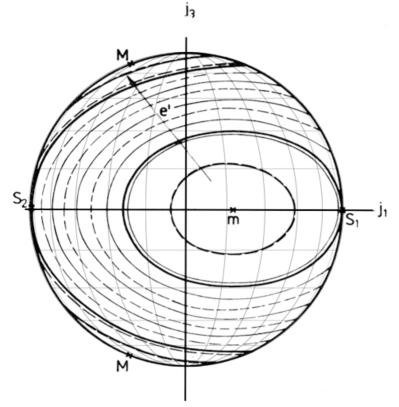
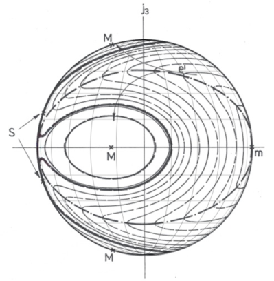
Figure 68: Routhians and classical orbits of an i_13/2 quasiparticle in the triaxial potential with $\varepsilon=0.26,\gamma=-30^{\circ}$, rotating with the frequency $\omega$ about the 1- axis, which is the medium axis. The layout is analog to Fig. 63.
Upper left panel: Quantal routhians for zero pairing.
Upper right panel: Quantal routhians for $\Delta=0.12~{}\hbar\omega_{0}$ and $\lambda=0$.
Lower left panel: Classical orbits in angular momentum space for zero pairing. The figure shows the medium-long-projection of the orbits, which lie on the surface of the sphere of fixed angular momentum. The frequency $\omega=0.025\omega_{0}$. The energy of the orbits increases in direction of the arrow.
Lower right panel: Analogous to the lower left panel for finite pairing. The dash-dotted line is the orbit with $e^{\prime}(0)=\lambda=0$.

In the following the 1-axis is chosen as the rotational axis, e.g $\vartheta=90^{\circ}$. From Eqs (169,A) it is clear that increasing the rotational frequency $\omega$ merely shifts the centers of the ellipses and hyperbolas along the 1-axis to $j_{1c}$ given by Eq. (172). Showing $\gamma=30^{\circ}$ as an example, the left panels of Fig. 67 illustrate the case $0^{\circ}\leq\gamma\leq 60^{\circ}$ of a particle in the triaxial potential that rotates about the short axis. The 1-3-projection of the orbits are hyperbolas. The asymptotes are the separatrix. Their crossing is the saddle point, which is the solution $j_{2}\not=0,~{}j_{1}=j_{1c},~{}j_{3}=j_{3c}=0$ of Eqs. (170,171). It has the energy

$$e^{\prime}_{S}=2\kappa\left[\sin\left(\gamma-30^{\circ}\right)j^{2}+\left(\frac{\omega}{\kappa}\right)^{2}\frac{1}{16\sqrt{3}\sin\gamma}\right].$$ (178)

As a new feature compared to the axial case, one has ”deformation assisted RAL”. The DALs orbits with $e^{\prime}_{m1}\leq e^{\prime}\leq e^{\prime}_{s}$ lie in the sector right to the separatrix. They revolve the 1-axis (s), which is also the rotational axis, i. e. they are RAL as well. The DALs orbits with $e^{\prime}_{m2}\leq e^{\prime}\leq e^{\prime}_{s}$ lie in the sector left to the separatrix. They also revolve the 1-axis (s), but they are anti-aligned with the s-axis. This region exists only for $-j_{1c}<j$, i. e. only as long as the center of the seperatrix lies inside the angular momentum sphere. The sectors above and below the separatrix contain the DALl orbits, which are two-fold degenerate. The topology is reflected by the routhians in the upper left panel of Fig. 67. Below the separatrix the orbits are aligned or anti-aligned with the s-axis. For $\omega/\kappa>j(4\sqrt{3}\sin\gamma)$ the center of the asymptotes lies outside the angular momentum sphere, and there are no anti-RAL orbits left. This is where the highest anti-aligned routhian meets the separatrix. Now the two-fold degenerate DAL orbits are located above a new separatrix, which is the hyperbola that touches the angular momentum sphere from inside. Like for the parabolas in the axial case, the curvature of the hyperbolas decreases with $\omega$. For $\omega\rightarrow\infty$ they approach vertical lines, and only RAL orbits survive. For $\gamma\rightarrow 0$ one has $j_{c}\rightarrow-\infty$, and the hyperbolas become parabolas. For $\gamma\rightarrow 60^{\circ}$, only DALs orbits remain, which are vertical lines and RAL.

The right panel of Fig. 66 displays how the quantal routhians and the stationary points of the classical routhian change with the triaxiality parameter $\gamma$ for a given frequency of $\omega=0.025\omega_{0}$. The zero-point energy of the lowest quantal routhian is larger for the DAL orbits at strong triaxility, which are well confined by the potential, than the RAL orbits at axial shape, which are less confined by the cranking term. The curve m1 shows the classical minimum of the anti-aligned RAL orbits in the $0^{\circ}\leq\gamma\leq 60^{\circ}$ sector. It is noted that m1 continues S of the axial case, both of which corresponding to the touch point of the orbit with the angular momentum sphere at $j_{1}=-j,~{}j_{3}=0$. The separatrix S, which corresponds to the center of the hyperbolas, branches off this curve at slightly positive $\gamma$ values. Understanding this in terms of geometry requires a more detailed analysis, which is omitted, because it is not particularly relevant.

The above discussion for $\gamma=0^{\circ}$ exemplifies the general relation between the quasiparticle and the particle orbits. Applying it to the case $\gamma=30^{\circ}$, consider the upper hemisphere $j_{3}>0$. (The lower hemisphere is symmetric.) Take the particle orbits obtained for $\Delta=0$ and overlay the Fermi orbit $e^{\prime}(\omega=0,j_{1},j_{3})=\lambda$ (dash-dotted). The branch of the quasiparticle orbit that lies above the Fermi orbit is particle-like and remains about the same. The branch that lies below the Fermi orbit is hole-like, i. e. it is obtained by reflection through the 2-3- plane. In the vicinity of the Fermi orbit the particle- and the hole-branches are bent such that they smoothly match, where the larger $\Delta$ the smoother the bend.

The lower right panel of Fig. 67 shows the quasiparticle orbits that emerge from the particle orbits in the lower left panel. For the displayed case of $\lambda=0$ the Fermi hyperbolas coincide with the dash-dotted asymptotes. The reflected hole-branches close the particle branches in the right hemisphere, which generates new orbits of FAL nature. The FAL region is separated by the separatrix S1 from the two disjunct RAL spaces, one on the right- and one on the left-hand side, having large and small alignment $\langle j_{1}\rangle$, respectively. They are separated by S2 from the DALl regions above and below and the anti-aligned RAL region to the left. The various regions are indicated in the routhian diagram in the upper right panel. The quasiparticle orbits for other values of $\lambda$ can be qualitatively constructed by reflecting the particle orbits through the Fermi orbit in the non-rotating potential with the energy $e=\lambda$, which are the hyperbolas away from the asymptotes in Fig. 65 right (see Fig. 65).

Showing $\gamma=-30^{\circ}$ as an example, the left panels of Fig. 68 illustrate the case $-60^{\circ}\leq\gamma\leq 0^{\circ}$ of an i_13/2 particle in the triaxial potential that rotates about the medium axis. The 1-3-projected orbits are ellipses. With increasing $\omega$ their center moves to the right to $j_{1c}$ given by Eqs. (172). There are two separatices S1 and S2, which are the ellipses that touch the circle right or left, respectively. The touching points are the solutions $j_{2}=j_{3}=0,~{}j_{1}=\pm j$ of Eqs. (170,171). Their energies are

$$e^{\prime}_{S1,S2}=-\frac{\kappa}{2}\sin\left(\gamma+30^{\circ}\right)j^{2}\pm\omega j.$$ (179)

Inside S1 ($e^{\prime}<e^{\prime}_{S1}$) lie the DALs orbits that revolve the s-axis and outside S2 ($e^{\prime}>e^{\prime}_{S2}$) lie the DALl orbits that revolve the l-axis. Between the separatrices a belt of RAL orbits is located. The two separatrices disappear for $\omega/\kappa>j|4\sqrt{3}\sin\gamma|$, when $j_{c}>j$, and only the RAL orbits remain. The topology is reflected by the routhians in the upper left panel of Fig. 68. Outside the separatrices one sees the doubly degenerate the DAL orbits with some anti-alignment (cf. discussion of $\gamma=0$), inside there are the signature-split RAL orbits. As a new feature, the RAL orbits do not carry much aligned angular momentum $\langle j_{1}\rangle$ when the RAL phase space is still small. The contributions of the right and left turning points are comparable because the orbits extend far to the left, where $j_{2}$ is small (see discussion for the axial case). With increasing $\omega$ the centers of the ellipses move to the right. The ellipse S1 shrinks and with it the phase space of the DALs orbits inside. RAL orbits with positive $\langle j_{1}\rangle$ emerge outside. Likewise, the ellipse S2 grows with $\omega$, the phase space of the DALl orbits outside shrinks, and RAL orbits with negative $\langle j_{1}\rangle$ emerge inside. For $\omega=-4\kappa\sqrt{3}j\sin\gamma$ the center of S1 reaches the surface of the sphere, and no DALs orbits remain. For $\omega=2\kappa\sqrt{3}j\cos(\gamma+30^{\circ})$ the curvature of S2 equals the one of the circle, and no DALl orbits remain. In case of $\gamma=-30^{\circ}$ the DAL orbits disappear at the common frequency $\omega=2\kappa\sqrt{3}j$.

For $\gamma\rightarrow 0^{\circ}$ the center $j_{c}\rightarrow\infty$ and $a_{1}/a_{3}\rightarrow 0$. The separatrix S1 disappears, the orbits become parabolas, and the above-discussed scenario for prolate shape is approached. Fig. 66 right demonstrates that slightly below $\gamma=0$ the separatrix S1 merges with the m, the minimum of the classical routhian, which continues as m to $\gamma>0$. For $\gamma\rightarrow-60^{\circ}$ the ellipses become circles, and the separatrix S2 disappears. The DALs orbits between m and S1 have minimal energy for oblate shape, which reflects their good overlap with the potential. In the RAL region the orbit that is maximally anti-aligned has the largest energy. With decreasing energy, the projection $\langle j_{1}\rangle$ becomes less negative and eventual positive. As seen in Fig. 66, with increasing $\omega$ the RAL belt opens from the $\omega=0$ - separatrix. The orbits nearby are weakly coupled to triaxial potential, because the orbits change from DALl to DALs at S. As a consequence the cranking term dominates the energy order.

Oblate shape and rotation about the l-axis is also realized for $\gamma=-180^{\circ}$. Compared to the prolate shape $\gamma=0^{\circ}$, this choice just changes the sign of the $j_{3}^{2}$ term, which is equivalent with $j_{1}\rightarrow-j_{1}$ and $e^{\prime}\rightarrow-e^{\prime}$. This corresponds to a reflection of orbits in the lower left panel of Fig. 63 through the 2-3-plane and a horizontal reflection of the upper left panel. The two alternative pictures correspond to different projections of the three-dimensional orbits. For $\gamma=-60^{\circ}$ the 1-3-projection is the l-l-projection, which gives shifted circles. For $\gamma=-180^{\circ}$ the 1-3-projection is the s-l-projection. The l-l-projection is obtained by eliminating $j_{3}^{2}$ for $j_{2}^{2}$ in Eq. (169), which results in orbits that are circles with centers on the 1-axis.

The lower right panel of Fig. 68 shows the quasiparticle orbits that emerge from particle orbits in the lower left panel. Qualitatively they are constructed by reflecting the particle orbits through the Fermi ellipse, which is shown by the dashed dotted curve, and connecting the reflected hole-branches inside with the particle branches outside. The reflection increases strongly the aligned angular momentum $\langle j_{1}\rangle$ of the lowest RAL orbits. The separatrix S is obtained by connecting the unpaired reflected separatrix S1 with S2 through the Fermi ellipse. Its saddle points S are close to S2 and the reflected saddle point S1. The DALl outside S2 retain their particle character while the DALs orbits inside S1 become holes. For the considered special case $\gamma=-30^{\circ}$ and $\lambda=0$ they are degenerate.

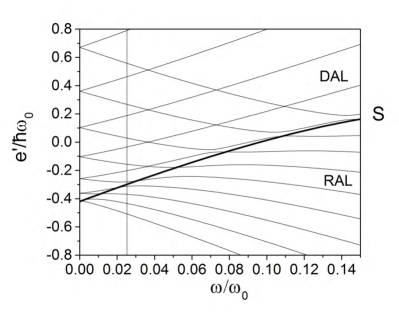
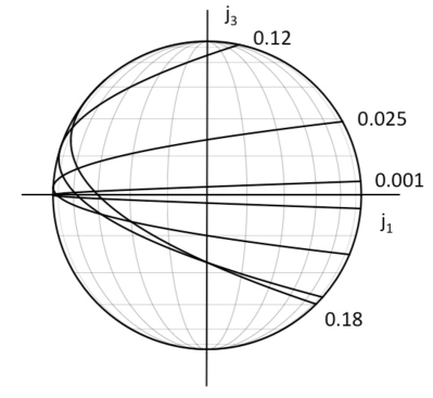
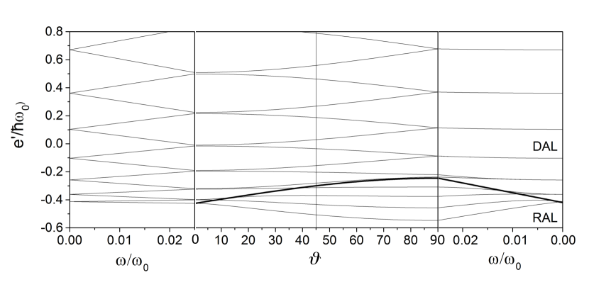
Figure 69: Upper left panel: Quantal routhians of an i_13/2 particle in the prolate potential $\varepsilon=0.26$ that rotates with the frequency $\omega$ about the axis that is tilted by $45^{\circ}$ into the 1-3-plane. Upper right panel: Separatrices of the classical orbits that belong to the left panel. Lower part middle panel: Quantal routhians as functions of the tilt angle $\vartheta$ at $\omega=0.025\omega_{0}$. The left and right panels show the routhians for rotation about the l- and s-axes, respectively. The layout is analog to Figs. 63, 64.

A.3 Rotation about a tilted axis

The upper left panel of Fig. 69 illustrates the case $\gamma=0$ of a prolate potential that rotates about an axis tilted by $45^{\circ}$ into the 1-3-plane, which is the plane spanned by the short axis and the long symmetry axis, respectively. The tilt shifts the axis of the parabolas to $j_{3c}=\cos\vartheta\omega/(6\kappa)$ and reduces the curvature to $6\kappa/(\sin\vartheta\omega)$, which can be seen in the upper right panel that shows how the separatrix changes with $\omega$. The DAL orbits outside the separatrix are no longer symmetric with respect to the 1-axis, and their routhians are no longer degenerate. At low frequency they are split by $-\omega\langle j_{3}\rangle\cos\vartheta$. The RAL orbits inside S revolve an axis that has the angle $\arcsin(j_{3c}/j)$ with the 1- axis. With increasing $\omega$ the curvature of the parabolas decreases and their axes move up. In this way, the upper DAL orbits cross over into the RAL space. The separatrix disappears for $\omega\approx 0.18\omega_{0}$ when the curvature of the parabola equals that of the circle at the touching point. There is no longer a topological difference between RAL and DAL. Increasing $\omega$ further the orbits approach straight lines with the slope $-\cot\vartheta$ (-1 for the displayed case), i. e. they approach the limit of a fixed angular momentum projection on the tilted axis. The lower panel of Fig. 69 illustrates how the quantal routhians change with $\vartheta$. Changing the tilt angle transforms the orbits from parabolas centered around the 1-axis for $\vartheta=90^{\circ}$ via parabolas with a reduced curvature centered around the $j_{3c}$ axis to horizontal lines for $\vartheta=0^{\circ}$. These DAL orbits are circles revolving the 3-axis with $j_{3}=\pm\Omega$ being the conserved angular momentum projection on the symmetry axis. They are also RAL orbits because the cranking axis agrees with the symmetry axis.

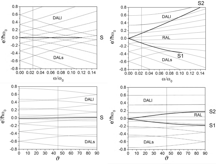
Figure 70: Quantal routhians of an i_13/2 particle in the triaxial potential with $\varepsilon=0.26,|\gamma|=30$, rotating with the frequency $\omega$ about a tilted axis. The layout is analog to Fig. 63.
Upper left panel: $\gamma=30^{\circ},~{}\vartheta=45^{\circ}$, rotation axis tilted into the s-l plane.
Upper right panel: $\gamma=-210^{\circ},~{}\vartheta=45^{\circ}$, rotation axis tilted into the m-s plane
Lower left panel: $\gamma=30^{\circ},~{}\omega=0.025\omega_{0}$.
The axis turns from the l- axis ($\vartheta=0$) to the s-axis ($\vartheta=\pi/2$).
Lower right panel: $\gamma=90^{\circ},~{}\omega=0.025\omega_{0}$.
The axis turns from the m- axis ($\vartheta=0$) to the s-axis ($\vartheta=\pi/2$).

For non-axial shape the centers of the particle orbits are shifted to $j_{1c}$ and $j_{3c}$ given by Eq. (172). The upper left panel of Fig. 70 shows the routhians for $\gamma=30^{\circ}$ and $\vartheta=45^{\circ}$ as an example for the rotation about an axis in the s-l-plane. The 1-3-projected orbits are hyperbolas. The asymptotes are the two separatrix branches, which cross at S located at $j_{1c}$ and $j_{3c}$. The lower left panel of Fig. 67 illustrates the case $\vartheta=90^{\circ}$. For $\vartheta<90^{\circ}$ S is moved up by $j_{3c}$(=$-j_{1c}$ for $\vartheta=45^{\circ}$). The DALs orbits right to S are also RAL orbits which revolve an axis that has the angle $\arcsin(j_{3c}/j)$ with the 1- axis. With increasing $\omega$ the center of S moves upward left on a straight line with the slope $-\cot\vartheta\sin\gamma/\cos(\gamma+30^{\circ})$ (-1 for the displayed case), which increases the phase space below the asymptote with the slope +1 at the expense of the phase space above it. This means that DALl orbits with $\langle j_{3}\rangle>0$ move into the DALs area and DALs orbits with $\langle j_{1}\rangle<0$ move into the DALl area. These are the routhians that cross the S line in Fig. 70 up-left. When the center of S reaches the angular momentum sphere at $j_{1c}^{2}+j_{3c}^{2}=j^{2}$ (at $\omega=0.12\omega_{0}$ for the shown case), the separatrix disappears, and all orbits become RAL revolving the tilted rotational axis. Increasing $\omega$ further, they approach straight lines with slope $-\cot\vartheta$ (-1 for the displayed case). The lower middle panel of Fig. 70 shows the routhians for $\omega=0.025\omega_{0}$ as a function of the tilt angle $\vartheta$ of the rotational axis. While the rotational axis is swept from the l- axis to the s- axis the center S of the asymptotes moves on a circle from the 3-axis to the 1- axis, where it is located in the lower left panel of Fig. 67. For $\vartheta=0$ the DALl orbits are also RALl split by $-\omega\langle j_{3}\rangle$, whereas the DALs orbits are disjunct and degenerate. Increasing $\vartheta$ the doublets split by $-\omega\sin\vartheta\langle j_{1}\rangle$. Decreasing $\vartheta$ from $90^{\circ}$ the analog appears, where DALl is exchanged with DALs. For $\gamma\rightarrow 0$, $j_{1c}$ moves far left and the hyperbolas become the parabolas of the axial case.

The 1-3-projection of the orbits corresponds to the m-l-projection for $-60^{\circ}\leq\gamma\leq 0^{\circ}$ and to the m-s-projection for $-240^{\circ}\leq\gamma\leq-180^{\circ}$ (cf. Table 2). As seen from Eqs. (A, 172), rotation about an axis that is tilted by $\vartheta$ with respect to the m- axis into the m-s- plane is related to rotation about an axis that is tilted by the same angle into the m-l-plane by the replacement $\{e^{\prime},~{}j_{1c},~{}j_{3c}\}\rightarrow\{-e^{\prime},~{}-j_{1c},~{}-j_{3c}\}$.

The upper right panel of Fig. 70 shows the routhians for $\gamma=-210^{\circ}$ and $\vartheta=45^{\circ}$ as an example for the rotation about an axis in the m-s-plane. The 1-3-projected orbits are ellipses with the center $j_{1c}$ and $j_{3c}$, which moves downward left on a straight line with the slope $-\cot\vartheta\sin\gamma/\cos(\gamma+30^{\circ})$ (1 for the shown case) with increasing $\omega$. The lower left panel of Fig. 68 shows the m-l-projection for rotation about the m-axis, i.e. $\vartheta=90^{\circ},~{}\gamma=-30^{\circ}$. The m-s-projection is obtained by reflecting through the 3-axis and exchanging maxima (M) and minima (m). For $\vartheta<90^{\circ}$ the two separatrices are the ellipses that touch the circle at S1 and S2 below the 1-axis. Between them lie the RAL orbits which revolve an axis that has the angle $\arcsin(-j_{3c}/j)$ with the 1-axis. While the points S1 and S2 move down on the circle with $\omega$ the RAL region grows at expense of the DAL regions. The DALs region shrinks faster than DALl region.

The outer separatrix S1 disappears when the curvature at the touching point is equal to the curvature of the circle, which occurs at $\omega=0.104\omega_{0}$ for the illustrated case (similar to the disappearance of the parabolic separatrix in the right panel of Fig. 69). For larger $\omega$ the RAL orbits approach straight lines with the slope $\cot\vartheta$. When the center reaches the angular momentum sphere at $j_{1c}^{2}+j_{3c}^{2}=j^{2}$ and the touching ellipse becomes a point, which occurs at $\omega=0.208\omega_{0}$ for the illustrated case, the inner separatix S2 disappears, and only RAL orbits remain. The lower right panel of Fig. 70 shows the routhians for $\gamma=-210^{\circ}$ and $\omega=0.025\omega_{0}$ as functions of the tilt angle, i. e. how they change from rotation about the s-axis to rotation about the m-axis. The development of the orbits can be anticipated from the lower left panel of Fig. 68. The center of the ellipses moves on a circle from the 1-axis to the 3-axis when $\vartheta$ changes from $90^{\circ}$ to $0^{\circ}$. The RAL region between the two ellipses shrinks on this path, which is reflected by the quantal routhians. For $\vartheta\rightarrow 0^{\circ}$ the two separatices merge into one ellipse that touches the circle on both sides, which is the 2-3-projection of the asymptotes in the lower left panel of Fig. 67 (rotated by $90^{\circ}$, M$\leftrightarrow$m).

As for rotation about the principal axes, the quasiparticle orbits can be qualitatively constructed from the particle orbits by reflection through the Fermi orbits.

A.4 Induced triaxiality and tilt angles

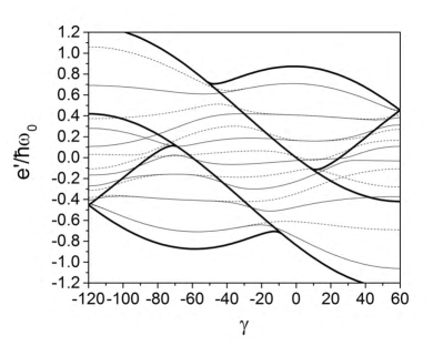
Figure 71: Routhians of an i_13/2 quasiparticle particle in the triaxial potential with $\varepsilon=0.26$ as function of the triaxiality parameter $\gamma$ rotating about the 1-axis with the frequency $\omega=0.025\omega_{0}$ (left panel) and $\omega=0.060\omega_{0}$ (right panel). The layout is analog to Fig. 63. The cases $\gamma=-30^{\circ},~{}0^{\circ},~{}30^{\circ}$ shown in Figs. 63 - 68 are marked. The separatrices and maxima and minima of the classical routhian are shown as thick curves and labeled in accordance with the other figures.

The triaxial deformation parameter $\gamma$ is susceptible to the polarization by the excited quasiparticles. The equilibrium value of $\gamma$ can be seen as the balance between the drive of the excited quasiparticles and the restoring force of the rotating ”core”, which is the configuration from which the quasiparticles or particles and holes are excited [159]. For a qualitative guess, which is often enough, it is sufficient to discuss the general trends. The balance between the coupling to the deformed potential, which favors a large overlap of the density distribution of the orbit with the deformed potential, and the inertial forces, which favor the alignment of the particle angular momentum with the rotation axis, determines the preferred $\gamma$ value and tilt angle $\vartheta$. To make a picture yourself of the density distribution, imagine the torodial density distribution of the high-j orbital (see Fig. 21) to be averaged over the various orientations corresponding to the classical orbits of $\vec{j}$.

Figs. 66 and 71 show the single particle routhians as functions of $\gamma$ for rotation about the principal 1-axis with two different frequencies. For $\omega=0$ the minimum of the lowest state in the shell lies at $|\gamma|=60^{\circ}$, because $\vec{j}$ of the classical orbit m is aligned with the symmetry s-axis, which makes best overlap with the potential (cf. Fig. 66 and discussion above). For finite $\omega$, $\gamma=+60^{\circ}$ is lower because m is aligned with the 1-axis (which is s), which gives the extra energy gain of $\omega j_{1}$. This is not the case for $\gamma=-60^{\circ}$, where m is aligned with the 2-axis (which is s). The rotational gain $\omega j_{1}$ is small for this DAL orbit, which corresponds to M in the lower left panel of Fig. 63 with $j_{1}\rightarrow-j_{1}$. Prolate $\rightarrow$ oblate is achieved by changing the sign of the $j_{3}^{2}$ term, which is equivalent with $e^{\prime}\rightarrow-e^{\prime}$ and $j_{1}\rightarrow-j_{1}$. For $\omega=0$ and triaxial shape the m orbit has DALs character. Its energy is higher than for oblate shape because the density torus overlaps better with the potential that has the two l axes in the torus’ plane instead of the axes m and l. For finite $\omega$, $\gamma>0$ is preferred because the m orbit is both DALs and RAL giving the extra energy gain $\omega j_{1}$ compared to $\gamma<0$, where the gain is small because it is DALs but not RAL (cf. Figs. 67 and 68).

The highest state appears as a hole in the inert filled shell, which has $e^{\prime}_{hole}=-e^{\prime}_{particle}$, i. e. its minima are the maxima of the particle states. As seen in the left panel of Fig. 66, the maxima of the M orbit lie at $\gamma=0^{\circ},~{}-120^{\circ}$ for $\omega=0$. The orbit with maximal energy has the smallest overlap with the potential: The axes s and s lie in the torus’ plane for prolate shape. For $\omega>0$, M at $\gamma=-120^{\circ}$ is shifted up by $\omega j_{1}$ because the $j_{1}$ is aligned with the symmetry axis l, whereas for $\gamma=0^{\circ}$ the term $\omega j_{1}$ is small (cf. Fig. 63). For triaxial shape the M orbit has DALl character. Its overlap with the potential is larger then for prolate shape, which is clear from geometry: The density torus overlaps less with the potential that has the axes s and s in the torus’ plane intend of the axes m and s. For finite $\omega$, $\gamma<-60^{\circ}$ is preferred because the M orbit is both DALl and RAL giving the extra upward shift of $\omega j_{1}$. For $-60^{\circ}<\gamma<0^{\circ}$, the shift is small because the orbit is DALs but not RAL.

As seen in the left panel of Fig. 66, the mid-shell states have a minimum at $\gamma=0^{\circ},~{}-120^{\circ}$ and a maximum at $\gamma=\pm 60^{\circ}$ for $\omega=0$. A mid-shell orbit is a circle in the 1-2-plane for axial shape, which means that the plane of the torus is rotated around the 3-axis. The resulting average density is strongly concentrated at the poles of the angular momentum sphere. Such dumbbell distribution has a good overlap with the prolate potential when its symmetry axis is aligned with the symmetry l-axis of the potential ($\gamma=0^{\circ}$). It has a poor overlap when its symmetry axis is aligned with the symmetry s-axis of the oblate potential ($\gamma=60^{\circ}$, in this case the symmetry axis is 1). When the stripe between the separatrices opens up with increasing $\omega$ the minima and maxima are shifted to triaxial shapes along with the separatrices (cf. Fig. 71).

The states that are DAL but not simultaneously RAL favor a tilt of the rotational axis away from the principal axis. As seen in the lower left panels of Figs. 63 - 68, these orbits have a large $\pm j_{3}$ projection but a small negative $j_{1}$ projection. The cranking term $-\omega(j_{1}\sin\vartheta+j_{3}\cos\vartheta)$ decreases with $\vartheta$ for the $j_{3}>0$ orbits. The RAL states favor rotation about the principal axis 1 when they have a substantial positive $j_{1}$ component, because the induced component $j_{3}=j_{3c}\propto\omega$ remains small. The lower panel of Fig. 69 illustrates this for axial shape. When $\vartheta$ changes from $90^{\circ}$ to $0^{\circ}$ the degenerate signature partners of the DAL orbits split rapidly because of the term $\mp\omega\cos\vartheta|j_{3}|$, where $|j_{3}|\approx\Omega$, which is the good angular momentum projection on the symmetry axis for $\vartheta=0^{\circ}$. The lower branch favors a finite tilt angle. The RAL orbits change to DAL orbits with a small projection $j_{3}$. They favor $\vartheta=90^{\circ}$ because the energy loss of $-\omega\sin\vartheta j_{1}$ is overcome by the gain in $-\omega\cos\vartheta j_{3}$.

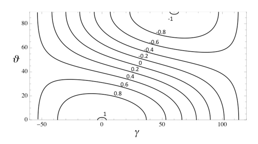
Figure 72: Location of the minimum of the lowest quasiparticle state with respect to the triaxiality parameter $\gamma$ and the tilt angle $\vartheta$ within the 1-3-plane. The curves correspond to different occupancy of the j-shell. The numbers indicate the ratio $\lambda/(2\kappa j^{2})$, where $\pm 2\kappa j^{2}$ are the minimal and maximal energy of a particle in the non-rotating potential.

For finite pairing, there is a simple relation between the energy minimum of the lowest quasiparticle with respect to $\gamma$ and $\vartheta$ and the chemical potential $\lambda$. For a given value of $\lambda$ the classical routhian (176) of the lowest quasiparticle orbit touches the angular momentum sphere. To good approximation the touching point is located at $e\left(j_{1},j_{3}=\sqrt{j^{2}-j_{1}^{2}}\right)=\lambda$, where

$$e^{\prime}(\gamma,\vartheta)=\Delta-\omega\left(j_{1}(\gamma)\sin\vartheta+j_{3}(\gamma)\cos\vartheta\right).$$ (180)

The routhian $e^{\prime}((\gamma,\vartheta)$ takes the lowest value when $\omega\left(j_{1}(\gamma)\sin\vartheta+j_{3}(\gamma)\cos\vartheta\right)=\omega j$, which according to Eq. (169) requires

$$\lambda=\kappa j^{2}\left[\left(3\cos^{2}\vartheta-1\right)\cos\gamma-\sqrt{3}\sin^{2}\vartheta\sin\gamma\right].$$ (181)

For all possible values of $\gamma$, the classical energy takes values values between $-2\kappa j^{2}$ and $2\kappa j^{2}$, which restricts $\lambda$ to this interval and suggests using the ratio $-1\leq\lambda/(2\kappa j^{2})\leq 1$ as a parameter that indicates the occupancy of the j-shell.

Fig. 72 shows the solutions of Eq. (181) for various shell occupancies. The region $-240^{\circ}\leq\gamma\leq-60^{\circ}$ is related to the shown region by $\gamma\rightarrow-60^{\circ}-\gamma$ and $\vartheta\rightarrow 90^{\circ}-\vartheta$. The upper edge corresponds to rotation about the 1-axis and the lower to rotation about the 3-axis. The solutions are respectively

$$\vartheta=90^{\circ}:\cos(\gamma-60^{\circ})=-\frac{\lambda}{2\kappa j^{2}},~{}~{}~{}\vartheta=0^{\circ}:\cos\gamma=\frac{\lambda}{2\kappa j^{2}}.$$ (182)

Depending on the $\gamma$ sector, they represents rotation about one of the principal axes. For the $\gamma$ value at the minimum the projection of $\vec{j}$ on the rotation axis takes the maximal value, which is $j_{1}=j$ or $j_{3}=j$ for $\vartheta=90^{\circ}$ and $\vartheta=0^{\circ}$, respectively. At bottom of the shell, where the quasiparticle orbit has the character of the lowest particle orbit, it drives the shape toward $\gamma=60^{\circ}$, i. e. rotation about the symmetry s-axis of oblate shape. At the top of the shell, where it has the character of a hole with the orbit of the highest particle, it drives the shape toward $\gamma=0^{\circ}$, i. e. rotation about the symmetry l-axis of prolate shape. A mid-shell quasiparticle drives toward $\gamma=-30^{\circ}$ for $\vartheta=90^{\circ}$, which is triaxial shape rotating about the m-axis ($\gamma=90^{\circ},~{}~{}\vartheta=0^{\circ}$ is the same solution).

As seen in Fig. 72, the tilt angle $\vartheta$ is the second degree of freedom to maximize the energy gain $-\vec{\omega}\cdot\vec{j}$. Away from the optimal $\gamma$ value the lowest quasiparticle has FAL character (see the lower right panels of Figs. 63 and 68)). Aligning the rotational axis $\vec{\omega}$ with the Fermi axis $\vec{j}_{\lambda}$ one achieves an energy gain of $\omega\left(\sin\vartheta j_{1\lambda}+\cos\vartheta j_{3\lambda}\right)$, where $j_{1\lambda}$ and $j_{3\lambda}$ can be estimated by the above-discussed reflection of the particle orbits through the Fermi orbit. The gain in changing $\gamma$ for $\vartheta=90^{\circ}$ is $\omega j_{1\lambda}$, where $j_{1\lambda}$ is the value for the FAL orbit at the non-optimal $\gamma$ value. In analogy, it is $\omega j_{3\lambda}$ for $\vartheta=0^{\circ}$. For the partially filled shell there is a wide range of optimal $\gamma-\vartheta$ combinations. Whether a change of $\gamma$ or $\vartheta$ or a combination is preferred depends on further excited quasiparticles and the quasiparticle vacuum.

Appendix B Table of content

1. Introduction	2
2. The Unified Model: virtues and limits	4
2.1. The Bohr Hamiltonian	5
2.2. The Deformed Shell Model	6
2.3. Deformed prolate nuclei	8
2.3.1 The strong coupling limit	10
2.3.2. Comparison with experiment	13
2.4. Spherical nuclei	21
2.5. Microscopic basis of the Unified Model	25
2.6. Transitional nuclei	30
2.7. Quasiparticle triaxial rotor model	31
2.8. Approaches beyond the Unified Model	32
3. Rotating mean field	34
3.1. Selfconsistent cranking model	36
3.2. Symmetries	45
3.2.1. Axis of rotation is a principal axis	47
3.2.2. Axis of rotation in a principal plane	47
3.2.3. Axis of rotation out of the principal planes	48
3.3. Rotational frequency	49
3.4. Calculation of the mean field shape	52
3.5. Geometry and rotational response of quasiparticle orbitals	53
3.6. Cranked Shell Model	56
3.6.1. Bands as quasiparticle configurations	59
3.6.2. Bandcrossings	59
3.6.3. Cranked Shell Model classification of bands	63
3.7. Cranked shell correction approach	67
3.8. Rotation about a tilted axis	69
3.8.1. The spinning clockwork picture	69
3.8.2. Appearance of tilted rotation	72
3.8.3. Tilted axis cranking solutions of axial nuclei	73
3.8.4. Approximate tilted axis cranking solutions	78
3.8.5. Change of symmetry	80
3.8.6. Tilted axis cranking solutions of triaxial nuclei	84
Wobbling	85
Transverse wobbling	86
Chirality	90

4. Emergence and disappearance of collective degrees of freedom	96
4.1. Band termination	97
4.2. Magnetic rotation	102
4.3. Shears geometry	110
4.4. Emergence of rotational bands	113
4.4.1. Coherence length	114
4.4.2. Regularity	116
4.4.3. Three examples	118
4.5. Tidal Waves	121
4.6. Coherence of the deformation degrees of freedom	123
5. Outlook	125
6. References	126
Appendix A. Semiclassical analysis of high-j quasiparticle states	132
A.1. Axial shape, rotation about the short axis	135
A.2. Triaxial shape, rotation about a principal axis	139
A.3. Rotation about a tilted axis	145
A.4. Induced triaxiality and tilt angles	149

References

- [1] N. Bohr and F. Kalckar, Mat. Fys. Medd. Dan. Vid. Selsk. 14, (no. 10) (1937).
- [2] 0. Haxel , J. H. D. Jensen and H. E. Suess, Phys. Rev. 75, 1766 (1949).
- [3] M. G. Mayer, Phys. Rev. 75, 1969 (1949).
- [4] A. Bohr, Mat. Fys. Medd. Dan. Vid. Selsk. 26, (no. 14) (1952).
- [5] A. Bohr and B. R. Mottelson, Mat. Fys. Medd. Dan. Vid. Selsk. 27, (no. 16) (1953).
- [6] A. Bohr and B. Mottelson Nuclear Structure Vol. II. Nuclear Deformations, (W. A. Benjamin Inc., London/Amsterdam; Don Mils, Ontario/Sydney/Tokyo; 1975).
- [7] K. Heyde and J. L. Wood, Phys. Scr. 91, 083008 (2016).
- [8] D. R. Bes, Phys. Scr. 91, 063010, (2016).
- [9] D. J. Rowe, Nuclear Collective Motion: Models and Theory, (2nd Ed., World Scientific Publishing Co. Pte. Ltd., Singapore 2010).
- [10] D. J. Rowe, J. L. Wood Fundamentals of Nuclear Models, (World Scientific Pub. Co. Pte. Ltd. Singapore, 2010).
- [11] A. Bohr, B. Mottelson Struktur der Atomkerne, Bd. II (Akademie-Verlag, Leipzig 1975).
- [12] M. E. Rose, Elementary Theory of Angular Momentum (J. Wiley & Sons, New York; 1957).
- [13] A. Bohr and B. Mottelson Nuclear Structure Vol. I. Single-Particle Motion, (W. A. Benjamin Inc. New York, Amsterdam, 1969).
- [14] S. Frauendorf, Rev. Mod. Phys. 73, 463, (2001).
- [15] S. Frauendorf, Int. J. Mod. Phys. E 38, 1541001 (2015).
- [16] S. Frauendorf, AIP Conference Proceedings 1753, 030001 (2016).
- [17] S.G. Nilsson, Mat. Fys. Medd. Dan. Vid. Selsk., 29 (no. 16) (1955).
- [18] S. G. Nilsson, C. F. Tsang, A. Sobiczewski, Z. Szymański, S. Wycech, C. Gustafson, I. Lamm, P. Möller, Björn Nilsson, Nucl. Phys. A 131, 1 (1969).
- [19] J. Dudek, Z. Szymanski and T. Werner, Phys. Rev. C 23, 920 (1981).
- [20] P. Möller and R. Nix, Atomic Data and Nuclear Data Tables, 59, 185 (1995).
- [21] J. Bardeen, L. N. Cooper and J. R. Schrieffer, Phys. Rev, 106, 162 (1957), Phys. Rev. 108, 1175 (1957).
- [22] S. G. Nilsson and I. Ragnarsson, Shapes and Shells in Nuclear Structure (Cambridge University Press: 1995).
- [23] P. Ring and P. Schuck, The Nuclear Many-Body Problem, (Springer, New York: 1980).
- [24] J. P. Blaizot and G. Ripka, Quantum Theory of Finite Systems (MIT Press Cambridge, Massasuchsetts/ London: 1986).
- [25] Evaluated Nuclear Structure Data File, [http://www.nndc.bnl.gov/ensdf/].
- [26] W. D. Kulp, J. L. Wood, P. E. Garrett, C. Y. Wu, D. Cline, J. M. Allmond, D. Bandyopadhyay, D. Dashdorj, S. N. Choudry, A. B. Hayes, H. Hua, M. G. Mynk, M. T. McEllistrem, C. J. McKay, J. N. Orce, R. Teng and S. W. Yates, Phys. Rev. C 77, 061301(R) (2008).
- [27] S. W. Yates, I. Y. Lee, N. R. Johnson, E. Eichler, L. L. Riedinger, M. W. Guidry, A. C. Kahler, D. Cline, R. S. Simon, P. A. Butler, P. Colombani, F. S. Stephens, R. M. Diamond, R. M. Ronningen, R. D. Hichwa, J. H. Hamilton and E. L. Robinson, Phys. Rev. C 21, 2366 (1980).
- [28] B. Kotiliński. D. Cline, A. Bäcklin, K.G. Helmer, A.E. Kavka, W.J. Kernan, E.G. Vogt and C.Y. Wu, R.M. Diamond A.O. Macchiavelli and M.A. Deleplanque, Nucl. Phys. A 517, 365 (1990).
- [29] L. D. Landau and E.M. Lifshitz, 1985, Statistical Physics, Third Edition, (Pergamon Press, Oxford/ New York/ Toronto/ Sydney/ Paris/ Frankfurt).
- [30] G. Alaga, Alder, A. Bohr and B. Mottelson, Kgl. Danske Videnskab. Selskab, Mat. Fys. Medd. 29, No. 9 (1955).
- [31] Z. Szymanski, Fast Nuclear Rotation (Clarendon, Oxford:1983).
- [32] G.B. Hagemann, H. Ryde, P. Bosetti, A. Brockstedt, H. Carlsson, L.P. Ekstöm, A. Nordlund, R.A. Bark, B. Herskind, S. Leoni, A. Bracco, F. Camera, S. Frattini, Nucl. Phys. A 618, 199 (1997).
- [33] D. De Frenne, Nucl. Data Sheets 67, 809 (1992).
- [34] F. Corminboeuf, T. B. Brown, L. Genilloud, C. D. Hannant, J. Jolie, J. Kern, N. Warr and S. W. Yates, Phys. Rev C 63, 014305 (2000).
- [35] M. Piiparinen, R. Julin, S. Juutinen, A. Virtanen, P. Ahonen, C. Fahlander, J. Hattula, A. Lampinen., T. Lönnroth, A. Maj, S. Mitarai, D. Müller, J. Nyberg, Nucl. Phys. A 565, 671 (1993).
- [36] A. D. Ayangeakaa, U. Garg, M. A. Caprio, M. P. Carpenter, S. S. Ghugre, R. V. F. Janssens, F. G. Kondev, J. T. Matta, S. Mukhopadhyay, D. Patel, D. Seweryniak, J. Sun, S. Zhu, and S. Frauendorf, Phys. Rev. Lett. 110, 102501 (2013).
- [37] M. A. Deleplanque, S. Frauendorf, V. V. Pashkevich, S. Y. Chu and A. Unzhakova, Phys. Rev. C 69, 044309 (2004).
- [38] M. Bender, P.-H. Heenen and P.-G. Reinhard, Rev. Mod. Phys., 75, 121 (2003).
- [39] P.-G. Reinhard, Phys. Scr. 91, 023002 (2016).
- [40] W Satuła and W.. Nazarewicz, Phys. Scr. 91, 023013 (2016).
- [41] J. L. Egido, Phys. Scr. 91, 073003 (2016).
- [42] J. Meng and P. Zhao, Phys. Scr. 91 063008 (2016).
- [43] S.-G. Zhou, Phys. Scr. 91, 063008, (2016).
- [44] V. M. Strutinsky, Nucl. Phys. A 95, 420 (1967), Nucl. Phys. A 122, 1 (1968).
- [45] M. Brack, Jens. Damgaard, A. S. Jensen, H. C. Pauli, V. M. Strutinsky and C. Y. Wong, Rev. Mod. Phys. 44, 320 (1972).
- [46] W. D. Meyers and W. J. Swiatecki, Annals of Phys., 55, 395 (1969).
- [47] S. T. Belyaev, Mat. Fys. Medd. Dan. Vid. Selsk. 31, No. 11 (1959).
- [48] D. R Inglis, Phys. Rev. 96, 1059 (1954), Phys. Rev. 97, 701 (1955).
- [49] M. Baranger and K. Kumar, Nucl. Phys. A 122, 241 (1968), Nucl. Phys. A 122, 273 (1968).
- [50] T. Niks̆ić, D. Vretenar, P. Ring, Prog. in Part. and Nucl. Phys. 66, 519 (2011).
- [51] K. Matsuyanagi, M. Matsuo, T. Nakatsukasa, K. Yoshida, N. Hinohara and K. Sato, Phys. Scr. 91, 063014 (2016).
- [52] D.J. Thouless, J.G. Valatin, Nucl. Phys. 31, 211 (1962).
- [53] J. P. Delaroche, M. Girod, J. Libert, H. Goutte, S. Hilaire, S. Pèru, N. Pillet and G. F. Bertsch, Phys. Rev. C 81, 014303 (2010).
- [54] T. Nakatsukasa, K. Matsuyanagi, M. Matsuzaki and Y. R. Shimizu, Phys. Scr. 91, 063014 (2016).
- [55] R. A. Broglia, P. F. Bortignon, F. Barranco, E. Vigezzi, A. Idini and G. Potel, Phys. Scr. 91, 063012 (2016).
- [56] Y. Sun, Phys. Scr. 91, 043005 (2016).
- [57] P. M. Walker and F. R. Xu, Phys. Scr. 91 013010 (2016).
- [58] J. A. Sheikh, G. H. Bhat, W. A. Dar, S. Jehangir and P. A. Ganai, Phys. Scr. 91, 063015 (2016).
- [59] D. R. Bes and R. A. Sorensen, Advances in Nucl. Phys. 2, 129 (1969) and early work cited therein.
- [60] M. A. Riley, J. Simpson and E. S. Paul, Phys. Scr. 91,123002 (2016).
- [61] S. Leoni and A. Lopez-Martens, Phys. Scr. 91, 063009 (2016).
- [62] R. Bengtsson and S. Frauendorf, Nucl. Phys. A 327, 139 (1979).
- [63] L. D. Landau and E.M. Lifshitz, Classical Mechanics, Third Edition, (Pergamon Press, Oxford/ New York/ Toronto/ Sydney/ Paris/ Frankfurt; 1985).
- [64] L. D. Landau and E.M. Lifshitz, Classical Fields, Third Edition, (Pergamon Press, Oxford/ New York/ Toronto/ Sydney/ Paris/ Frankfurt; 1985).
- [65] B. Mottelson, Proc. Sym. on High-Spin Phenomena in Nuclei, Argonne, 1979, Report ANL/PHY-79-4.
- [66] S. Frauendorf, Contemporary research topics in nuclear physics, (Proc. of workshop on Nuclear Physics, Drexel University, Sep. 1-3 1980 (Plenum Press NY, 1982), p1.
- [67] S. Frauendorf, Phys. Scri. 24, 349 (1981).
- [68] I. Hamamoto and B. Mottelson, Phys. Lett. B 127, 281 (1983).
- [69] S. Frauendorf and E. Sobeslavsky, Collective motion and giant resonances: proceedings of the XVth Mikolajki Summer School on Nuclear Physics, Mikolajki, Poland, September 5-17,1983.
- [70] R. Bengtsson and S. Frauendorf, Nucl. Phys. A 314, 27 (1979).
- [71] R. Bengtsson, S. Frauendorf and F. R. May, At. Data and Nucl. Data Tables, 35, 15 (1986).
- [72] F. S.Stephens and R. S. Simon, Nucl. Phys. A 183, 257 (1972).
- [73] M. A. Riley and P. Pipidis, available at: http://physics.fsu.edu/TheBackBender.
- [74] I. Hamamoto, Nucl. Phys. A 271, 15 (1976).
- [75] R. S. Nikam, P. Ring, Y. Sun, E.R. Marshalek, Phys Lett. B 235, 215 (1990) and earlier work cited.
- [76] I. Y. Lee, S. Asztalos, M.-A. Deleplanque, B. Cederwall, R. M. Diamond, P. Fallon, A. O. Macchiavelli, L. Phair, F. S. Stephens, G. J. Wozniak, S. G. Frauendorf, J. A. Becker, E. A. Henry, P. F. Hua, D. G. Sarantites, J. X. Saladin and C. H. Yu, Phys. Rev. C 56, 753 (1997).
- [77] Ts. Venkova, W. Gast, R. M. Lieder, D. Bazzacco, G. de Angelis, E. O. Lieder, A. A. Pasternak, R. Menegazzo, S. Lunardi, C. Rossi Alvarez, C. Ur, T. Martinez, M. Axiotis, D. Napoli, W. Urban, T. Rzaca-Urban, S. Frauendorf, Eur. Phys. J. A 26, 19 (2005).
- [78] K. Neergård, V. V. Pashkevich and S. Frauendorf, Nucl. Phys. A 262, 61 (1976).
- [79] C. G. Andersson, S.E. Larsson, G. Leander, .P. Möller, S. G. Nilsson, I. Ragnarsson, .S. Åberg, Nucl. Phys. A 268, 205 (1976).
- [80] P. J. Twin, B. M. Nyakó, A. H. Nelson, J. Simpson, M. A. Bentley, H. W. Cranmer-Gordon, P. D. Forsyth, D. Howe, A. R. Mokhtar, J. D. Morrison, J. F. Sharpey-Schafer and G. Sletten, Phys. Rev. Lett. 57, 811 (1986).
- [81] P. Fallon, A. Alderson, M.A. Bentley, A.M. Bruce, P.D. Forsyth, D. Howe, J.W. Roberts, J.F. Sharpey-Schafer, P.J. Twin, F.A. Beck, T. Byrski, D. Curien, C. Schuck, Phys. Lett. B 218, 137 (1989).
- [82] R. Wyss, (1999) contact R. Wyss, e-mail: wyss@msi.se.
- [83] T. R. Werner and J. Dudek, 1992, Atomic Data and Nuclear Data Tables 50, 179 (1992), ibid. 59,1 (1995).
- [84] A.V. Afanasjev, D.B. Fossan, G.J. Lane, I. Ragnarsson, Phys. Rep., 322, 1 (1999).
- [85] R. Bengtsson, www.matfys.lth.se/ ragnar.
- [86] D. Vretenar, A. V. Afanasjev, G. A. Lalazissis and P. Ring, Phys. Rep. 409, 101259 (2005).
- [87] S. Frauendorf, Nucl. Phys. A 557 259c (1993).
- [88] S. Frauendorf, Nucl. Phys. A 677, 115 (2000).
- [89] P. Olbratowski, J. Dobaczewski, J. Dudek and W. Płóciennik, Phys. Rev. Lett. 93, 052501 (2004).
- [90] P. Olbratowski, J. Dobaczewski and J. Dudek, Phys. Rev. C 73, 054308 (2006).
- [91] J. Peng, J. Meng, P. Ring and S. Q. Zhang, Rev. C 78, 024313 (2008).
- [92] P.W. Zhao, S.Q. Zhang, J. Peng, H.Z. Liang, P. Ring, J. Meng, Phys. Lett. B 699, 181 (2011).
- [93] M. Danos and V. Gillet, 1967, Phys. Rev. 161, 1034.
- [94] B. Riemann, 1860, Abh. Kön. Ges. Wiss. (Göttingen) 9, 1 (1860).
- [95] S. Frauendorf, Phys. Scr. T125, 1(2005).
- [96] I. Hamamoto and H. Sagawa, Nucl. Phys. A 327, 99 (1979).
- [97] A. Brockstedt, J. Lyttkens-Lind n, M. Bergström, L.P. Ekström, H. Ryde, J.C. Bacelar, J.D. Garrett, G.B. Hagemann, B. Herskind, F.R. May, P.O. Tj m, S. Frauendorf, Nucl. Phys. A 571, 337 (1994).
- [98] S. Frauendorf, J. Meng and J. Reif, Proceedings of the Conference on Physics from Large -Ray Detector Arrays, Berkeley 1994 (LBL-35687, CONF-940888) Vol. 2, p. 52.
- [99] F. Dönau and S. Frauendorf in High Angular Momentum Properties of Nuclei, Oak Ridge 1983, Nuclear Science Research Conference Series, Vol. 4, edited by N.R. Johnson, (Harwood, New York) p. 143 (1983).
- [100] F. Dönau, Nucl. Phys. A 471, 469 (1987).
- [101] S. Frauendorf and J. Meng, 1997, Z. Phys. A 356, 263 (1996).
- [102] L. Grodzin, Ann. Rev. Nuclear Science, 18, 291 (1968).
- [103] S. Raman, C. W. Nestor, JR. and P. Tikkanen, At. Data and Nucl. Data Tables 78, 1 (2001).
- [104] H. Röpke and P. M. Endt, 1998, Nucl. Phys. A 632, 173 (1998).
- [105] H. Röpke, Nucl. Phys. A 674 , 95 (2000).
- [106] P. Möller, R. Bengtsson, B. G. Carlsson, P. Olivius and T. Ichikawa, Phys. Rev. Lett. 87, 162502 (2006).
- [107] C. Petrache, S. Frauendorf, M. Matsuzaki, R. Leguillon, T. Zerrouki, S. Lunardi, D. Bazzacco, C. A. Ur, E. Farnea, C. Rossi Alvarez, R. Venturelli and G. de Angelis, Phys. Rev. C 86, 044321 (2012).
- [108] S. Frauendorf, F. Dönau, Phys. Ref. C89, 014322 (2014).
- [109] I. Hamamoto, Phys. Scr. 91, 023004 (2016)
- [110] J. T. Matta, U. Garg, W. Li, S. Frauendorf, A. D. Ayangeakaa, D. Patel, K. W. Schlax, R. Palit, S. Saha, J. Sethi, T. Trivedi, S. S. Ghugre, R. Raut, A. K. Sinha, R. V. F. Janssens, S. Zhu, M. P. Carpenter, T. Lauritsen, D. Seweryniak, C. J. Chiara, F. G. Kondev, D. J. Hartley, C. M. Petrache, S. Mukhopadhyay, D. V. Lakshmi, M. K. Raju, P. V. Madhusudhana Rao, S. K. Tandel, S. Ray and F. Dönau, Phys. Rev. Lett. 114, 082501 (2015).
- [111] Y. R. Shimizu, T. Shoji and M. Matsuzaki, Phys. Rev. C 77, 024319 (2008) and earlier work cited therein.
- [112] S. Frauendorf, F. Dönau, Phys. Ref. C92, 064306 (2015).
- [113] V. Dimitrov, S. Frauendorf and F. Dönau, Phys. Rev. Lett. 84, 5732 (2000).
- [114] S. Frauendorf, F. Dönau, Phys. Rev. C, to be published.
- [115] S. Frauendorf and J. Meng, Nucl. Phys. A 617, 131 (1997).
- [116] D. Almehed, S. Frauendorf, F. Dönau, Phys. Ref. C 83, 054308 (2011).
- [117] S. Zhu, U. Garg, B. K. Nayak, S. S. Ghugre, N. S. Pattabiraman, D. B. Fossan, T. Koike, K. Starosta, C. Vaman, R. V. F. Janssens, R. S. Chakrawarthy, M. Whitehead, A. O. Macchiavelli and S. Frauendorf, Phys. Rev. Lett. 91, 132501 (2003).
- [118] S. Mukhopadhyay, D. Almehed, U. Garg, S. Frauendorf, T. Li, P. V. Madhusudhana Rao, X. Wang, S. S. Ghugre, M. P. Carpenter, S. Gros, A. Hecht, R. V. F. Janssens, F. G. Kondev, T. Lauritsen, D. Seweryniak and S. Zhu, Phys. Rev. Lett.99, 172501 (2007).
- [119] B. Qi , S.Q. Zhang, J. Meng, S.Y. Wang, S. Frauendorf, Phys. Lett. B 675, 175 (2009).
- [120] J. A. Alcántara-Núñez, J. R. B. Oliveira, E. W. Cybulska, N. H. Medina, M. N. Rao, R. V. Ribas, M. A. Rizzutto, W. A. Seale, F. Falla-Sotelo, K. T. Wiedemann, V. I. Dimitrov and S. Frauendorf, Phys. Rev. C 69, 024317 (2004).
- [121] J. Timár, P. Joshi, K. Starosta, V.I. Dimitrov, D.B. Fossan, J. Molnár, D. Sohler, R. Wadsworth, A. Algora, P. Bednarczyk, D. Curien, Zs. Dombrádi, G. Duchene, A. Gizon, J. Gizon, D.G. Jenkins, T. Koike, A. Krasznahorkay, E.S. Paul, P.M. Raddon, G. Rainovski , J.N. Scheurer, A.J. Simons, C. Vaman, A.R. Wilkinson, L. Zolnai, S. Frauendorf, Phys. Lett. B 598, 178 (2004).
- [122] A. D. Ayangeakaa, U. Garg, M. D. Anthony, S. Frauendorf, J. T. Matta, B. K. Nayak,D. Patel, Q. B. Chen, S. Q. Zhang, P.W. Zhao, B. Qi, J. Meng, R.V. F. Janssens, M. P. Carpenter, C. J. Chiara, F. G. Kondev, T. Lauritsen, D. Seweryniak, S. Zhu, S. S. Ghugre and R. Palit, Phys. Rev. Lett. 110, 172504 (2013).
- [123] S. J. Zhu, J. H. Hamilton, A. V. Ramayya, P. M. Gore, J. O. Rasmussen, V. Dimitrov, S. Frauendorf, R. Q. Xu, J. K. Hwang, D. Fong, L. M. Yang, K. Li, Y. J. Chen, X. Q. Zhang, E. F. Jones, Y. X. Luo, I. Y. Lee, W. C. Ma, J. D. Cole, M. W. Drigert, M. Stoyer, G. M. Ter-Akopian, A. V. Daniel, Eur. Phys. J. A 25, 459 (2005).
- [124] Y.X. Luo, S.J. Zhu, J.H. Hamilton, J.O. Rasmussen, A.V. Ramayya, C. Goodin, K. Li, J.K. Hwang, D. Almehed, S. Frauendorf, V. Dimitrov, Jing-ye Zhang, X.L. Che, Z. Jang, I. Stefanescu, A. Gelberg, G.M. Ter-Akopian, A.V. Daniel, M.A. Stoyer, R. Donangelo, J.D. Cole, N. J. Stone, Phys. Let. B 670, 307 (2009).
- [125] K. Starosta and T Koike, Phys. Scr. 92, 093002 (2017).
- [126] J. Meng, Q. B. Chen and S. Q. Zhang, Int. J. of Mod. Phys. E 23, 1430016 (2014).
- [127] W.A. Dar, J.A. Sheikh, G.H. Bhat, R. Palit, R.N. Ali, S. Frauendorf, Nucl. Phys. A 933, 123 (2015).
- [128] I. Ragnarsson, in Proceedings of the International Conference on The Nucleus: New Physics for the New Millenium, NAC, Faure, South Africa, 2000 edited by F. D. Smit, R. Lindsay and S. V. Föstrich (Kluwer Academic/Plenum, New York).
- [129] R. Wadsworth, R.M. Clark, J.A. Cameron, D.B. Fossan, I.M. Hibbert, V.P. Janzen, R. Krücken, G.J. Lane, I.Y. Lee, A.O. Macchiavelli, C.M. Parry, J.M. Sears, J.F. Smith, A.V. Afanasjev and I. Ragnarsson, 1998, Phys. Rev. Lett. 80, 1174 (1998).
- [130] G. Baldsiefen, H. Hübel, D. Mehta, B. V. Thirumala Rao, U. Birkental, G. Fröhlingsdorf, M. Neffgen, N. Nenoff, S.C. Pancholi, N. Singh, W. Schmitz, K. Theine, P. Willsau, H. Grawe, J. Heese, H. Kluge, K.H. Maier, M. Schramm, R. Schubart, H.J. Maier, Phys. Lett. B 275, 252 (1991).
- [131] B. Fant, R. J. Tanner, P. A. Butler, A. N. James, G. D. Jones, R. J. Poynter, C. A. White, K. L. Ying, D. J. G. Love, J. Simpson and K. A. Connell, J. Phys. G.. Nucl. Part. Phys. 17, 319 (1991).
- [132] Rod Clark and Bob Wadsworth, Phys. World 11 (7) 25 (1998).
- [133] R. M. Clark and A.O. Macchiavelli, 2000, Ann. Rev. Nucl. Part. Sci., 50, 1 (2000).
- [134] H. Hübel, Prog. Part. Nucl. Phys. 54, 1 (2005).
- [135] J. Meng, J. Peng, S. Q. Zhang, P. W. Zhao, Front. Phys. 8, 55 (2013).
- [136] R. M. Clark, S. J. Asztalos, G. Baldsiefen, J. A. Becker, L. Bernstein, M. A. Deleplanque, R. M. Diamond, P. Fallon, I. M. Hibbert, H. Hübel, R. Krücken, I. Y. Lee, A. O. Macchiavelli, R. W. MacLeod, G. Schmid, F. S. Stephens, K. Vetter, R. Wadsworth and S. Frauendorf, Phys. Rev. Lett. 78, 1868 (1997).
- [137] G. Baldsiefen, H. Hübel, W. Korten, D. Mehta, N. Nenoff, B.V. Thirumala Rao, P. Willsau, H. Grawe, J. Heese, H. Kluge, K.H. Maier, R. Schubart, S. Frauendorf and H.J. Maier, 1994, Nucl. Phys. A 574, 521 (1994).
- [138] S. Chmel, S. Frauendorf and H. Hübel, Phys. Rev. C 75, 044309 (2007).
- [139] S. Frauendorf, J. Meng and J. Reif, Proc. Conf. on Phys. from Large Gamma Ray Detector Arrays . Berkeley (August 1994), report LBL-35687, Vol. 2, 52.
- [140] Amita, A. K. Jain and B. Singh, Atomic Data and Nuclear Data Tables 74, 283 (2000).
- [141] F. Brandolini, M. Ionescu-Bujor, N.H. Medina, R.V. Ribas, D. Bazzacco, M. De Poli, P. Pavan, C. Rossi Alvarez, G. de Angelis, S. Lunardi, D. De Acu a, D.R. Napoli, S. Frauendorf, Phys. Lett. B 388, 468 (1996).
- [142] A. A. Pasternak, E. O. Podsvirova, R. M. Lieder, S. Chmel, W. Gast, Ts. Venkova, H. M. Jäger, L. Mihailescu, G. de Angelis, D. R. Napoli, A. Gadea, D. Bazzacco, R. Menegazzo, S. Lunardi, W. Urban, Ch. Droste, T. Morek, T. Rzaca-Urban, G. Duch ne, A. Dewald, Eur. Phys. J. A 23, 191 (2005).
- [143] R. M. Clark, S. J. Asztalos, B. Busse, C. J. Chiara, M. Cromaz, M. A. Deleplanque, R. M. Diamond, P. Fallon, D. B. Fossan, D. G. Jenkins, S. Juutinen, N. Kelsall, R. Kr cken, G. J. Lane, I. Y. Lee, A. O. Macchiavelli, R. W. MacLeod, G. Schmid, J. M. Sears, J. F. Smith, F. S. Stephens, K. Vetter, R. Wadsworth and S. Frauendorf, Phys. Rev. Lett. 82, 3220, (1999).
- [144] D. G. Jenkins, R. Wadsworth, J. A. Cameron, R. M. Clark, D. B. Fossan, I. M. Hibbert, V. P. Janzen, R. Kr cken, G. J. Lane, I. Y. Lee, A. O. Macchiavelli, C. M. Parry, J. M. Sears, J. F. Smith and S. Frauendorf, Phys. Rev. L ett. 83, 500 (1999).
- [145] H. Schnare, R. Schwengner, S. Frauendorf, F. Dönau, L. Käubler, H. Prade, A. Jungclaus, K. P. Lieb, C. Lingk, S. Skoda, J. Eberth, G. de Angelis, A. Gadea, E. Farnea, D. R. Napoli, C. A. Ur and G. Lo Bianco, Phys. Rev. Lett. 82, 4408 (1999).
- [146] A. O. Macchiavelli, R.M. Clark, M.A. Deleplanque, R.M. Diamond, P. Fallon, I.Y. Lee, F.S. Stephens, and K. Vetter, Phys. Rev. C 58, 3746 (1998).
- [147] A. O. Macchiavelli, R.M. Clark, M.A. Deleplanque, R.M. Diamond, P. Fallon, I.Y. Lee, F.S. Stephens and K. Vetter, Phys. Rev. C 58, R621 (1998).
- [148] A. O. Macchiavelli, R.M. Clark, P. Fallon, M.A. Deleplanque, R.M. Diamond, R. Krücken, I.Y. Lee, F.S. Stephens, S.J. Asztalos, B. Busse, R.W. MacLeod, G.J. Schmid, K. Vetter, D. Ward, Phys. Rev. C 57, R1073 (1998).
- [149] P. Van Isacker and A. O. Macchiavelli, Phys. Rev. C 87, 061301(R) (2013).
- [150] A. J. Simons, R. Wadsworth, D. G. Jenkins, R. M. Clark, M. Cromaz, M. A. Deleplanque, R. M. Diamond, P. Fallon, G. J. Lane, I. Y. Lee, A. O. Macchiavelli, F. S. Stephens, C. E. Svensson, K. Vetter, D. Ward and S. Frauendorf, Phys. Rev. Lett. 91, 0162501 (2003).
- [151] N. W. Ashcroft and N. D. Mermin, Solid State Physices, (Brooks and Cole 1976).
- [152] Frauendorf, S., D. Janssen, and L. Münchow,, Phys. Lett. 34B 469 (1971).
- [153] S. Frauendorf, Y. Gu, J. Sun, arXiv-id: 0709.0254 (2010).
- [154] S. Frauendorf, Y. Gu, J. Sun, Int. J. Mod. Phys. E 20, 465 (2011).
- [155] A. D. Ayangeakaa, U. Garg, M. A. Caprio, M. P. Carpenter, S. S. Ghugre, R. V. F. Janssens, F. G. Kondev, J. T. Matta, S. Mukhopadhyay, D. Patel, D. Seweryniak, J. Sun, S. Zhu and S. Frauendorf, Phys. Rev. Lett. 110, 102501 (2013).
- [156] A. O. Macchiavelli, A. D. Ayangeakaa, S. Frauendorf, U. Garg and M. A. Caprio, Phys. Rev. C 90, 047304 (2014).
- [157] A. Chakraborty, J. N. Orce, S. F. Ashley, B. A. Brown, B. P. Crider, E. Elhami, M. T. McEllistrem, S. Mukhopadhyay, E. E. Peters, B. Singh and S. W. Yates, Phys. Rev. C 83, 034316 (2011).
- [158] R. F. Casten and N.V. Zamfir, Phys. Rev. Lett. 87, 052503 (2001).
- [159] S. Frauendorf and F. R. May, Phys. Lett. B125, 254 (1983).