Massive outflow properties suggest AGN fade slowly

Abstract

Massive large-scale AGN outflows are an important element of galaxy evolution, being a way through which the AGN can affect most of the host galaxy. However, outflows evolve on timescales much longer than typical AGN episode durations, therefore most AGN outflows are not observed simultaneously with the AGN episode that inflated them. It is therefore remarkable that rather tight correlations between outflow properties and AGN luminosity exist. In this paper, I show that such correlations can be preserved during the fading phase of the AGN episode, provided that the AGN luminosity evolves as a power law with exponent $\alpha_{\rm d}\sim 1$ at late times. I also show that subsequent AGN episodes that illuminate an ongoing outflow are unlikely to produce outflow momentum or energy rates rising above the observed correlations. However, there may be many difficult-to-detect outflows with momentum and energy rates lower than expected from the current AGN luminosity. Detailed observations of AGN outflow properties might help constrain the activity histories of typical and/or individual AGN.

1 Introduction

Kiloparsec-scale outflows of molecular gas have been observed in numerous galaxies (Feruglio et al., 2010; Rupke & Veilleux, 2011; Sturm et al., 2011; Alatalo et al., 2011; Cicone et al., 2014), with mass outflow rates $\dot{M}>1000\;{\rm M_{\odot}}$ yr^-1 and velocities $v_{\rm out}>1000$ km s^-1. The properties of these outflows are well explained by the AGN wind-driven outflow model (King, 2003, 2010; King & Pounds, 2015), which posits that a mildly relativistic wind originating in the AGN accretion disc inflates a large-scale outflow by transferring its kinetic energy rate $\dot{E}_{\rm kin}\mathrel{\raise 1.29167pt\hbox{$\sim$}\mkern-14.0mu\lower 1.72218pt\hbox{$-$}}0.05L_{\rm AGN}$ to the surrounding interstellar medium (ISM). The velocities, kinetic energy and momentum rates of the observed outflows (Cicone et al., 2014) agree very well with analytical predictions (Zubovas & King, 2012a). In at least one case (Tombesi et al., 2015), both a small-scale relativistic wind and a large-scale molecular outflow are detected in the same galaxy, with their kinetic energies agreeing with analycial predictions (however, see Veilleux et al., 2017, for a re-examination of these results, finding a smaller average outflow mass, momentum and energy rate over a longer flow timescale of $\sim 10$ Myr).

These close correlations are typically considered evidence that winds of the observed AGN drive the observed outflows. However, on closer inspection, this simple interpretation is unlikely to be correct. AGN winds are highly intermittent, with lifetimes of only a few months (King & Pounds, 2015). AGN are observed to change their luminosity significantly on timescales from from several years (Gezari et al., 2017) to several times $10^{4}$ yr (Keel et al., 2017). The crossing timescale of the outflow is, however, $t_{\rm dyn,out}\sim R_{\rm out}/v_{\rm out}\sim 1R_{\rm kpc}v_{3}^{-1}$ Myr, with $R_{\rm out}\equiv 1R_{\rm kpc}$ kpc and $v_{\rm out}\equiv 10^{3}v_{3}$ km s^-1. Therefore, the outflows that are observed at distances beyond $\sim 0.1$ kpc from the galactic nucleus are unlikely to have been inflated by the current AGN episode. In fact, it is expected that an outflow would persist for an order of magnitude longer than the duration of the AGN phase that inflated it (King et al., 2011). During this time, other AGN episodes might occur in the galaxy, but there is no a priori reason why these should have luminosity values correlating as well with the outflow properties as observed ones do.

In this paper, I investigate the possible solutions to this issue, considering outflow properties as potential constraints on the AGN luminosity evolution. First of all, in Section 2, I briefly review the AGN wind outflow model and present the possibilities for maintaining correlations between outflows and AGN. The most promising possibility is that on long timescales, the AGN luminosity tends to vary in such a way that correlations are preserved. I investigate this possibility in Section 3, finding that if the AGN luminosity fades as a power law over time, as suggested by some evolutionary models, the correlations with outflow properties can be preserved during the fading phase as well as the driving phase. I discuss the implications of the results in Section 4 and conclude in Section 5.

2 Outflows in fading AGN

2.1 Wind outflow model

The model of AGN outflows driven by accretion disc winds was proposed by King (2003) in order to explain the observed $M-\sigma$ correlation (Ferrarese & Merritt, 2000). It is based on the fact that accretion disc radiation can drive a quasi-relativistic ($v_{\rm w}\sim 0.1c$) wide-angle wind, also known as an ultra-fast outflow (UFOs). The wind tends to self-regulate to keep the outflow rate $\dot{M}_{\rm w}$ similar to the SMBH accretion rate (King, 2010). The wind energy rate is then

$$L_{\rm w}=\frac{\dot{M}_{\rm w}v_{\rm w}^{2}}{2}=\frac{\eta}{2}L_{\rm AGN}\mathrel{\raise 1.29167pt\hbox{$\sim$}\mkern-14.0mu\lower 1.72218pt\hbox{$-$}}0.05L_{\rm AGN},$$ (1)

where $\eta\mathrel{\raise 1.29167pt\hbox{$\sim$}\mkern-14.0mu\lower 1.72218pt\hbox{$-$}}0.1$ is the radiative efficiency of accretion.

The wind shocks against the surrounding interstellar medium (ISM) and drives a large-scale outflow. Depending on the distance between the AGN and the wind shock, the wind might be cooled efficiently by the AGN radiation field via the inverse-Compton process, leaving only the wind momentum to push against the gas. However, this critical ‘cooling radius’ is probably so small as to be irrelevant (Faucher-Giguère & Quataert, 2012; Bourne & Nayakshin, 2013), and the shocked wind is always essentially adiabatic. In this case, the outflow is energy-driven - it has the same energy rate as the wind (eq. 1). Such an outflow is capable of removing most of the gas from the galaxy spheroid. The predicted relation between the properties of the outflow and the AGN luminosity agree very well with observations (Zubovas & King, 2012a; Cicone et al., 2014). For a more detailed review of the model, see King & Pounds (2015).

The model, as presented above, assumes that the AGN luminosity is fixed at either some constant fraction of $L_{\rm Edd}$ or at zero. However, this is clearly unrealistic: if an outside reservoir ceases feeding the central SMBH, its accretion disc gets depleted on a viscous timescale, and the AGN luminosity should decrease over a finite amount of time as well, perhaps of order $10^{4}-10^{5}$ yr (Schawinski et al., 2010; Ichikawa et al., 2016; Keel et al., 2017). The outflow, meanwhile, continues to expand and coast (King et al., 2011). Before it dissipates completely, several more AGN episodes can occur, with potentially different maximum luminosities. The existence of AGN-outflow correlations suggests either that outflows can only be observed during the driving AGN phase, or that correlations between AGN luminosity and outflow properties are maintained during the fading phase and during subsequent AGN episodes.

2.2 Outflow observability

The simplest solution to the problem would be that outflows are only observed at times when illuminated by powerful AGN, and become unobservable almost as soon as the AGN begins fading. That way, all observed outflows would be inflated by the AGN of the same luminosity as observed, and thus their properties would correlate with the AGN luminosity. This may be the case for UFOs. Their sizes are $\ll 1$ pc (Tombesi et al., 2012, 2013), giving a light-travel time of $<1$ yr. Therefore, one might expect UFOs to dissipate, recombine and become essentially unobservable in tandem with the fading of the central source, on timescales as short as several tens of years (Ichikawa & Tazaki, 2017).

Massive kpc-scale outflows, on the other hand, should persist and be detectable long after the AGN fades. The shock-ionised gas in the outflows recombines and cools down rapidly (Zubovas & King, 2014), leading to somewhat lower typical momentum and kinetic energy rates of ionised outflows compared with molecular ones (Fiore et al., 2017). However, even ionised gas can be detectable on timescales of several times $10^{4}$ yr after the AGN fades (Keel et al., 2017). Outflowing molecular gas should remain kinematically distinct from the rest of the galactic material for a long time, up to an order of magnitude longer than the duration of the driving AGN phase (King et al., 2011), assuming that it was kinematically distinct in the first place, i.e. that the outflow velocity was much higher than the gas velocity dispersion in the host galaxy.

At some point after the AGN begins fading, it becomes unobservable. Then the remaining outflow might be identified as being driven by star formation, since no AGN would be visible in the host galaxy of the outflow. However, during the intermediate fading phase, the outflow can still be identified as being driven by the AGN. It seems unlikely, given the evidence above, that the AGN outflow would become undetectable very soon after the AGN begins dimming.

2.3 Conditions for outflow existence

Another reason limiting the possible variations of the correlations is a sort of cosmic coincidence. The presence of massive outflows requires two conditions that limit the time range during which they can appear.

First of all, the driving AGN must be luminous enough. The critical luminosity is $L_{\rm crit}\mathrel{\raise 1.29167pt\hbox{$\sim$}\mkern-14.0mu\lower 1.72218pt\hbox{$-$}}L_{\rm Edd}\left(M_{\sigma}\right)$, where $M_{\sigma}\mathrel{\raise 1.29167pt\hbox{$\sim$}\mkern-14.0mu\lower 1.72218pt\hbox{$-$}}3.68\times 10^{8}\sigma_{200}^{4}{\rm M_{\odot}}$ is the critical SMBH mass, corresponding rather well to the observed $M-\sigma$ relation (King, 2010; Zubovas & King, 2012b). This means that massive outflows can only occur once the SMBH grows beyond a critical mass (King, 2005), i.e. the presence of the outflow implies that the SMBH is already on the $M-\sigma$ relation or close to it.

On the other hand, a molecular outflow can only form if the host galaxy contains large amounts of gas. However, the outflow sweeps that gas out of the host, so any subsequent significant episodes of AGN activity are unlikely to produce massive outflows. In fact, our Galaxy may be evidence of this: the Fermi bubbles (Su et al., 2010) are most likely inflated by a recent AGN episode (Zubovas & Nayakshin, 2012) and are thus analogous to the outflows in other galaxies. However, due to the low gas mass in the bulge and halo of the Milky Way, the bubbles are only visible in gamma rays and would be almost impossible to detect in other galaxies, even though they should exist in the majority of them (King et al., 2011). In fact, it was only very recently that Fermi bubble analogues were detected in M31 (Pshirkov et al., 2016).

These two constraints strongly suggest that we only observe outflows during a very particular time in a given galaxy’s evolution - the time when the central SMBH has recently reached its mass as given by the $M-\sigma$ relation and is now driving an outflow that would shut off both star formation in the spheroid and subsequent SMBH growth.

Even if this is the case, the outflow persists an order of magnitude longer than the AGN episode which inflated it (King et al., 2011). During this time, there may be several more AGN episodes in the host galaxy, which can illuminate the existing outflow and be observed simultaneously. Even during a single AGN episode, the correlation with outflow properties can in principle be broken. A typical AGN phase probably lasts only $t_{\rm q}\sim 5\times 10^{4}-2\times 10^{5}$ yr (Schawinski et al., 2015; King & Nixon, 2015), followed by a fading phase of duration $t_{\rm d}\sim$ a few times$10^{4}$ yr (Keel et al., 2017). During this phase, the correlations between outflow and AGN properties might be disrupted. However, the time for which the outflow properties would appear abnormally large compared with the AGN luminosity is $>t_{\rm d}$, giving a probability of observing abnormally large outflow properties $p>t_{\rm d}/\left(t_{\rm d}+t_{\rm q}\right)\sim 0.5$. Given that abnormally large values are not commonly observed, either $t_{\rm d}$ must be very short, so that AGN fade away extremely abruptly, or AGN luminosity must decrease slower than exponentially. The first possibility appears unlikely, since the AGN is fed via a disc, which takes a finite time to dissipate.

2.4 Viscous evolution of AGN feeding rate

AGN accretion discs evolve and are depleted on a viscous timescale

$$t_{\rm visc}\sim\frac{1}{\alpha_{\rm visc}}\left(\frac{H}{R}\right)^{-2}t_{\rm dyn}\sim 600M_{8}\left(\frac{R}{R_{\rm ISCO}}\right)^{3/2}{\rm yr}.$$ (2)

Here, $M_{8}\equiv M_{\rm SMBH}/10^{8}{\rm M_{\odot}}$ and $R_{\rm ISCO}\sim 3R_{\rm Schw}$ is the radius of the innermost stable circular orbit. For a $10^{8}{\rm M_{\odot}}$ black hole, the viscous timescale at the outer edge of the accretion disc, which is at $R\mathrel{\raise 1.29167pt\hbox{$\sim$}\mkern-14.0mu\lower 1.72218pt\hbox{$-$}}0.01$ pc$\mathrel{\raise 1.29167pt\hbox{$\sim$}\mkern-14.0mu\lower 1.72218pt\hbox{$-$}}700R_{\rm ISCO}$ (King & Pringle, 2007), is

$$t_{\rm visc,0.01{\rm pc}}\mathrel{\raise 1.29167pt\hbox{$\sim$}\mkern-14.0mu\lower 1.72218pt\hbox{$-$}}1.2\times 10^{8}{\rm yr}.$$ (3)

The characteristic disc evolution timescale should lie somewhere between these two extremes. King & Nixon (2015) estimate that the typical duration of an AGN event should be a few times $10^{5}$ yr. One can then assume that the accretion disc is depleted and the AGN luminosity fades on a similar timescale $t_{\rm q}$. The precise shape of the luminosity function is then (King & Pringle, 2007)

$$L_{\rm AGN}\left(t\right)=L_{\rm Edd}\left(1+\frac{t}{t_{\rm q}}\right)^{-19/16},$$ (4)

which shows a power-law decay at late times.

A power-law decay of AGN luminosity seems a promising possibility for keeping the outflow properties correlating with $L_{\rm AGN}$, since analytical calculations show that stalling outflow properties also evolve as power laws in time (King et al., 2011).

2.5 Section summary

The arguments given above suggest that:

• AGN outflows should remain detectable while the AGN fades and long afterward, although they will not necessarily be identified as AGN-driven outflows if the AGN is too weak;

• There is a non-negligible probability of detecting an outflow in a galaxy with a fading AGN;

• The AGN luminosity is likely to decay as a power law at late times.

In order to determine whether the outflow correlations can be maintained in such systems, I performed a numerical investigation of outflow propagation in galaxies with flickering AGN. The results are presented in the next Section.

3 Simulated outflows in fading AGN

3.1 Numerical model

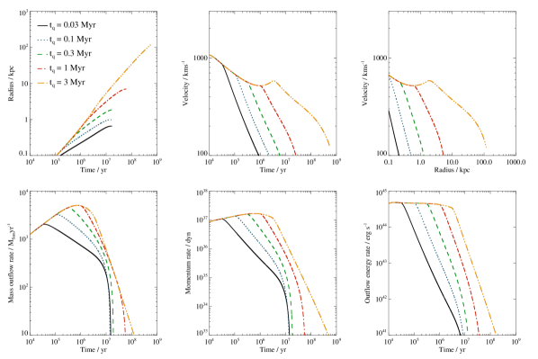
Figure 1: Evolution of outflow parameters in simulations with a single activity episode, followed by immediate complete shutdown of the AGN. From left to right, top to bottom, the panels show time evolution of radius, time evolution of velocity, velocity against radius, time evolution of the mass outflow rate, time evolution of the momentum rate and time evolution of the outflow kinetic energy rate. The five simulations have different quasar activity durations, as labelled in the top-left panel.

Figure 2: Same as Figure 1, but for simulations with exponential decay of AGN luminosity. Thin lines in the last two panels show the ratio between outflow momentum (bottom middle) or kinetic energy (bottom right) rate and the corresponding AGN parameter, $L_{\rm AGN}/c$ or $L_{\rm AGN}$ respectively, with scale on the right. Values of the free parameters $t_{\rm q}$ and $t_{\rm d}$ are labelled in the top-left panel.

I numerically integrate the equation of motion of an energy-driven AGN wind outflow. The equation is derived based on three assumptions:

• Matter in the galaxy is distributed spherically symetrically;

• The outflow is perfectly adiabatic;

• The outflow does not have significant velocity gradients and therefore moves as a single entity.

The validity of these assumptions is discussed in Section 4.3 below. The equation can then be derived using an appropriate formulation of Newton’s second law:

$$\frac{{\rm d}}{{\rm d}t}\left[M\dot{R}\right]=4\pi R^{2}P-\frac{GM\left[M_{\rm b}+M/2\right]}{R^{2}}$$ (5)

and the energy equation:

$$\frac{{\rm d}}{{\rm d}t}\left[\frac{3}{2}PV\right]=\frac{\eta}{2}L_{\rm AGN}-P\frac{{\rm d}V}{{\rm d}t}-\frac{{\rm d}E_{\rm g}}{{\rm d}t},$$ (6)

In these equations, $M(R)$ is the instantaneous swept–up gas mass being driven out when the outflow contact discontinuity is at radius $R$, $P$ is the expanding gas pressure and $M_{\rm b}$ is the mass of the stars and dark matter within $R$ (these are left unmoved by the outflow). The outflowing material is assumed to be distributed approximately uniformly in a shell between $R$ and the outer shock at $4R/3$ (cf. Zubovas & King, 2012a); this assumption has no effect on the results presented here, as I am only considering integrated quantities of the outflow. The energy equation expresses the change of internal energy of the outflow (left-hand side) as a balance between energy input by the AGN with luminosity $L_{\rm AGN}$, the $p$d$V$ work of outflow expansion and the work against gravity.

A detailed derivation of the equation of motion is presented in Zubovas & King (2016). Here, I just quote the final result:

$$\begin{split}\dddot{R}&=\frac{\eta L_{\rm AGN}}{MR}-\frac{2\dot{M}\ddot{R}}{M}-\frac{3\dot{M}\dot{R}^{2}}{MR}-\frac{3\dot{R}\ddot{R}}{R}-\frac{\ddot{M}\dot{R}}{M}\\ &+\frac{G}{R^{2}}\left[\dot{M}+\dot{M}_{\rm b}+\dot{M}\frac{M_{\rm b}}{M}-\frac{3}{2}\left(2M_{\rm b}+M\right)\frac{\dot{R}}{R}\right].\end{split}$$ (7)

Here, $\dot{M}\equiv\dot{R}\partial M/\partial R$ and $\ddot{M}\equiv\ddot{R}\partial M/\partial R+\dot{R}({\rm d}/{\rm d}t)\left(\partial M/\partial R\right)$. In the rest of the paper, I refer to the first term on the right hand side of equation (7) as the driving term, the next four terms as the kinetic terms, and the terms involving the gravitational constant $G$ as the gravity term.

This equation is then integrated numerically, using a specified history of nuclear activity $L_{\rm AGN}\left(t\right)$, assuming a central SMBH of mass $M_{\rm BH}=2\times 10^{8}\;{\rm M_{\odot}}$, giving an Eddington luminosity $L_{\rm Edd}=1.3\times 10^{46}$ erg/s. The actual histories investigated are presented at the beginning of Section 3.2.

The matter distribution in the galaxy consists of two components. The first component is an $M_{\rm h}=6\times 10^{11}\;{\rm M_{\odot}}$ halo, which has an NFW (Navarro et al., 1997) density profile with virial radius $r_{\rm vir}=200$ kpc and concentration parameter $c=10$ and is composed almost purely of dark matter and stars, with a gas fraction of only $f_{\rm g,h}=10^{-3}$. The second component is the bulge, with a Hernquist density profile with scale radius $r_{\rm b}=1$ kpc, total mass $M_{\rm b}=4\times 10^{10}\;{\rm M_{\odot}}$ and a large gas content $f_{\rm g,b}=0.8$. The effect of this matter distribution is that the outflow tends to accelerate significantly when it moves outside $R\sim 3$ kpc, if the AGN is still active at that time. The outflow starts at a radius $R_{0}=10$ pc with a velocity $v_{0}=200$ km s^-1, which is approximately the expected velocity dispersion in the bulge. The propagation of the outflow does not depend strongly on the initial conditions (King et al., 2011).

3.2 Results - single activity episode

Figure 3: Same as Figure 2, but for simulations with power-law decay of AGN luminosity.

Figure 4: Same as Figure 2, but for simulations with extended power-law decay of AGN luminosity.

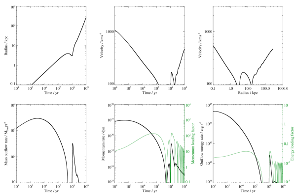
Figure 5: Outflow parameters in simulation with multiple AGN episodes, each of duration $t_{\rm q}=10^{5}$ yr, separated by $t_{\rm rep}=10^{8}$ yr, following an extended power-law decay of the AGN luminosity. Thin green lines in the last two panels show the momentum and energy loading factors.

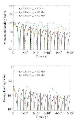
Figure 6: Momentum (top) and energy (bottom) loading factors in simulations with multiple AGN episodes, with different characteristic episode durations $t_{\rm q}$ and repetition timescales $t_{\rm rep}$, following an extended power-law decay of the AGN luminosity.

Figure 7: Same as Figure 6, but for AGN episodes with shorter characteristic durations.

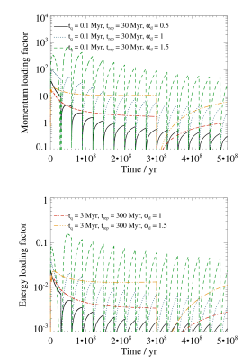
Figure 8: Same as Figure 6, but for AGN episodes with power law decay with different exponents $\alpha_{\rm d}$.

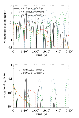
Figure 9: Same as Figure 6, but AGN episodes have progressively smaller initial luminosities, starting at $L_{\rm Edd}$ and decreasing by factor $3$ with each episode.

I present the results of numerical calculations of outflow propagation, starting from the simplest possible AGN luminosity history: a single event with luminosity $L=L_{\rm Edd}$, lasting for a duration $t_{\rm q}$, after which the AGN turns off forever. This is clearly an unrealistic situation, but it helps determine the timescales over which the properties of a coasting outflow evolve.

Next, I consider three possibilities of AGN luminosity decay: exponential, power-law and extended power-law. In the first case, approximately following the model of Haehnelt & Rees (1993), the AGN luminosity is described as

$$L_{\rm AGN}\left(t\right)=\begin{cases}L_{\rm Edd},&t<t_{\rm q},\\ L_{\rm Edd}\;{\rm exp}\left(\frac{t_{\rm q}-t}{t_{\rm d}}\right),&t>t_{\rm q},\end{cases}$$ (8)

where $t_{\rm d}$ is the luminosity decay timescale, a free parameter.

The power-law decay of AGN luminosity is described as follows:

$$L_{\rm AGN}\left(t\right)=\begin{cases}L_{\rm Edd},&t<t_{\rm q},\\ L_{\rm Edd}\left(\frac{t}{t_{\rm q}}\right)^{-\alpha_{\rm d}},&t>t_{\rm q},\end{cases}$$ (9)

where the exponent $\alpha_{\rm d}$ is a free parameter.

Finally, the extended power-law decay is based on the prediction by King & Pringle (2007), which is given above in eq. (4). I repeat it here for ease of reference:

$$L_{\rm AGN}\left(t\right)=L_{\rm Edd}\left(1+\frac{t}{t_{\rm q}}\right)^{-19/16}.$$ (10)

With this prescription, the AGN remains in an active state, defined by $L>0.01L_{\rm Edd}$ (e.g., Shankar et al., 2013), for $t_{\rm ep}\mathrel{\raise 1.29167pt\hbox{$\sim$}\mkern-14.0mu\lower 1.72218pt\hbox{$-$}}47t_{\rm q}$. King & Pringle (2007) use a characteristic timescale $t_{\rm q}\sim$ a few times $10^{5}$ yr, although a somewhat shorter timescale might be necessary to keep the total duration of the AGN episode in line with observations (Schawinski et al., 2010; Ichikawa et al., 2016; Keel et al., 2017).

All model AGN luminosity histories have a free parameter $t_{\rm q}$, with exponential and power-law histories having one more free parameter, respectively $t_{\rm d}$ or $\alpha_{\rm d}$. For simulations with only one free parameter, I calculate outflow propagation with $t_{\rm q}=0.03,0.1,0.3,1$ and $3$ Myr. For the exponential decay simulations, I use $t_{\rm q}=0.3$ and $3$ Myr and $t_{\rm d}=0.1,0.3$ and $3$ Myr. For the power-law decay simulations, I use $t_{\rm q}=0.3$ and $3$ Myr and $\alpha_{\rm d}=0.5,1$ and $2$. As seen in the figures below, all outflows take $\sim 10^{7}$ yr or longer to reach $R\sim 10$ kpc, which is the largest size of most observed outflows (Spence et al., 2016; Fiore et al., 2017), so each of the model systems would undergo at least a few, and perhaps several tens of, AGN episodes before the outflow would dissipate into obscurity and be no longer detectable.

Figures 1, 2, 3 and 4 show the evolution of main observable outflow parameters with time in the four groups of models: immediate AGN shutdown, exponential luminosity decay, power-law decay and extended power-law decay, respectively. For the sake of clarity, I omit the case $t_{\rm q}=3$ Myr, $t_{\rm d}=0.1$ Myr from the exponential decay plots, because this case shows an even more extreme decay of outflow parameters than $t_{\rm q}=3$ Myr, $t_{\rm d}=0.3$ Myr, with a corresponding extreme increase in the loading factors. Similarly, the case $t_{\rm q}=3$ Myr, $\alpha_{\rm d}=0.5$ is omitted from the power-law decay plots, because its evolution is very similar to that of $t_{\rm q}=0.3$ Myr, $\alpha_{\rm d}=0.5$.

The parameters shown are outflow radius $R$ (top left panels), outflow velocity $v$ (top middle panels), velocity against radius (top right), mass outflow rate $\dot{M}$(bottom left), momentum rate $\dot{M}v$ (bottom middle) and kinetic energy rate $\dot{M}v^{2}/2$ (bottom right). In Figures 2, 3 and 4, the last two panels also show the ratio between the outflow property in question and the corresponding AGN property, $L_{\rm AGN}/c$ or $L_{\rm AGN}$, showing the ‘loading factors’ of the outflow.

In the immediate shutdown simulations (Figure 1), the outflow velocity decays approximately as $t^{-\beta}$, with $\beta\in\{0.3;0.6\}$. The fastest decay occurs when the AGN activity duration is shortest. This is caused by two effects: closer to the centre of the galaxy, the potential well is deeper, requiring more work to lift the gas, and the gas density is higher, stopping the outflow more efficiently. The mass outflow rate decreases much faster than velocity, and faster in the outflows inflated by longer AGN activity episodes, because of the decrease in the gas density. Other parameters are a function of $\dot{R}$ and $\dot{M}$. In particular, the outflow momentum rate decay has a power-law exponent with $\beta_{\rm\dot{p}}\in\{1.0;2.0\}$, and the kinetic energy rate has $\beta_{\rm\dot{E}}\in\{1.5;2.2\}$. The important observation here is that all these parameters decay approximately as power-law functions. This suggests that a power-law decay of AGN luminosity might preserve the AGN-outflow correlations, while an exponential one might not.

Simulations with exponential AGN luminosity decay (Figure 2) confirm this suspicion. Independently of the precise value of the luminosity decay timescale $t_{\rm d}$, the outflow momentum and energy rates decay far slower than the AGN luminosity, leading to very large momentum and energy loading factors. When these factors increase to extremely high values ($\dot{p}c/L_{\rm AGN}\ga 10^{3}$, $\dot{E}/L_{\rm AGN}>1$), the outflow might no longer be identified as AGN-driven. If there is a powerful starburst happening in the galaxy (perhaps even triggered by the same outflow, cf. Silk, 2005; Zubovas et al., 2013), the outflow might be classified as driven by star formation, especially at $t>10^{7}$ yr, when the momentum and energy rates have decreased significantly and are similar to the typical starburst-driven outflow parameter values (Cicone et al., 2014; Geach et al., 2014; Heckman et al., 2015). Given that the outflow material cools down and some of it might not be detected, the estimated rates may be smaller than the true ones and the outflow properties might begin to resemble those of star-formation driven outflows earlier than $10^{7}$ yr after the beginning of the AGN phase. At intermediate times, however, outflows should be observed and correctly classified as AGN-driven; for example, the model with $t_{\rm q}=0.3$ Myr and $t_{\rm d}=0.1$ Myr (black solid line) spends $\sim 0.9$ Myr at $L>0.01L_{\rm Edd}$, out of which $0.4$ Myr, i.e. almost half the time, is spent with $\dot{p}c/L_{\rm AGN}>100$. This fraction is even higher if $t_{\rm d}/t_{\rm q}$ is higher. The lack of observed outflows with very large momentum or energy loading factors indicates that exponential decay of AGN luminosity is rare, if not non-existent.

Simulations with power-law decay of AGN luminosity (Figure 3) show momentum and energy loading factors that generally fall within the range of observed values. Momentum loading in most cases stays between $10$ and $10^{2}$ for more than $10^{7}$ yr after the AGN starts to dim. Only when the AGN activity is short and decay very rapid (green dashed lines) does the momentum loading factor increase to more than $10^{2}$, but this happens only at a time when the AGN luminosity has decreased by a factor $10^{2}-10^{3}$, so it is questionable whether such an outflow would be identified as AGN-driven in the first place. Another effect worth noting is that a slow decay of AGN luminosity can sometimes lead to the outflow breaking out of the galaxy anyway (black solid and red dot-dashed lines), since it provides enough energy to the gas for it to escape from the gravitational potential well.

Finally, the extended power-law simulations (Figure 4) result in even less variation of the momentum and energy loading factors. The kinetic energy rate of the outflow is in all cases $<10\%$ of the AGN luminosity, while the momentum rate only becomes higher than $100L_{\rm AGN}/c$ in the two simulations with the shortest activity duration $t_{\rm q}$. I conclude that this type of AGN luminosity evolution function is the best, of the three tested ones, at explaining the continued existence of tight correlations between AGN luminosity and outflow parameters even during the AGN decay phase.

3.3 Results - repeating activity episodes

Using the extended power-law model of AGN luminosity decay, I test the effect of the AGN experiencing several episodes of activity. At first, for simplicity, I assume that each episode reaches the same maximum luminosity equal to the Eddington value. The full luminosity function is then characterised by two free parameters: $t_{\rm q}$ and the time between the beginnings of two successive activity episodes, $t_{\rm rep}$.

With this luminosity function, the duty cycle $f_{\rm d}$ of the AGN, if defined as the fraction of time for which the AGN is brighter than some fraction $f$ of its Eddington luminosity, is given by

$$f_{\rm d}=\left(f^{-16/19}-1\right)\frac{t_{\rm q}}{t_{\rm rep}}=10^{-3}\left(f^{-16/19}-1\right)\frac{t_{\rm q,5}}{t_{\rm rep,8}},$$ (11)

where in the second equality I scale $t_{\rm q}$ and $t_{\rm rep}$ to $10^{5}$ and $10^{8}$ yr, respectively. Using a canonical AGN definition of $f=0.01$ (e.g., Shankar et al., 2013) gives $f_{\rm d}=0.047$, in reasonable agreement with observations (Kauffmann et al., 2003; Xue et al., 2010).

Figure 5 shows plots of the major outflow parameters in the simulation with $t_{\rm q}=10^{5}$ yr and $t_{\rm rep}=10^{8}$ yr. The outflow stalls and begins collapsing back before the second AGN episode; this adiabatic oscillation was removed from single-episode plots, because it is unlikely to occur in reality due to fragmentation of the outflowing gas. Subsequent AGN episodes push the outflowing gas out of the galaxy. Crucially, the momentum and energy loading factors (green lines in the last two panels) generally stay within the observationally-constrained bounds: $\dot{p}c/L_{\rm AGN}<100$, $\dot{E}/L_{\rm AGN}<0.05$. When the outflow moves beyond a few tens of kpc, the mass outflow rate becomes negligible and the outflow is unlikely to be detected. This happens after only 2-3 AGN episodes, supporting the notion that AGN outflows clear gas out of galaxies in a comparatively short time (Zubovas & King, 2012a).

Variations of the momentum and energy loading factors are shown in Figures 6 and 7 for outflows with different values of $t_{\rm q}$ and $t_{\rm rep}$. I use a linear scale for time, cut off at $t_{\rm max}=500$ Myr in Figure 6 and at $t_{\rm max}=100$ Myr in Figure 7, because subsequent episodes generally show very similar results. In the five simulations with $t_{\rm q}\geq 0.1$ Myr (Figure 6), the momentum loading factors do not exceed $200$, generally staying below a few tens. The energy loading factors are always below $5\%$ and do not rise above $2\%$ in most AGN episodes. In the simulations with shorter $t_{\rm q}<0.1$ Myr (Figure 7), both momentum and energy loading factors rise to higher values, reaching as much as $10^{3}$ for momentum loading. However, these outflows have very low velocities, $v_{\rm out}<200$ km/s, and therefore are unlikely to be distinguished from the random motions of gas in the host galaxy.

The extended power-law simulations all have the same exponent governing AGN luminosity decay, so I ran several tests with simple power-law AGN luminosity evolution in order to determine the importance of the exponent. The results are qualitatively similar to those of the extended power-law simulations and single-episode power-law simulations (Figure 3). Some example results are given in Figure 8. The exponent of the AGN luminosity decrease is a key factor governing the maximum momentum/energy loading factors reached. With exponent $\alpha_{\rm d}=0.5$, the AGN luminosity decreases so slowly that the momentum loading factor stays below $\sim 5$ after $t=30$ Myr, and the energy loading factor is $<1\%$. With $\alpha_{\rm d}=1.5$, the momentum loading factor increases to more than $100$, while the energy loading factor is $\sim 10\%$. When $\alpha_{\rm d}=1$, both the momentum and energy loading factors are very similar to those in the extended power law simulation. This should be expected, because the extended power law simulation has AGN luminosity decreasing with a power-law exponent $-19/16$, i.e. close to $-1$, at late times. If the AGN activity episodes are very long, both momentum and energy loading factors remain small, despite a rapid decrease in AGN luminosity.

3.4 Results - varied-luminosity episodes

Finally, I run a simulation with multiple AGN episodes of different starting luminosity. I take the characteristic durations $t_{\rm q}$ and repetition timescales $t_{\rm rep}$ to be the same as in the first group of simulations with multiple Eddington-limited extended power law episodes (presented in Figure 6). The only difference between the episodes is that only the first activity episode has a starting luminosity $L=L_{\rm Edd}$. Each subsequent episode has a starting luminosity three times lower than the previous one, but not lower than $0.03L_{\rm Edd}$. This represents a situation where the first activity episode drives an outflow which removes most of the gas from the central parts of the galaxy, and subsequent activity episodes are unable to fuel the AGN very efficiently. Each subsequent episode removes some more of the leftover gas, and so the maximum AGN luminosity decreases further.

The resulting momentum and energy loading factors are presented in Figure 9. In simulations with $t_{\rm q}=0.1$ Myr, the momentum loading factors rise to rather large values, $>10^{2}$ and even $>10^{3}$ in some instances. This suggests that in some cases, old outflows illuminated by a low-luminosity AGN can have very large formal momentum-loading factors, although this happens because the outflow momentum rates are inherited from previous, more luminous, AGN episodes. The low-luminosity AGN is unable to accelerate the outflow significantly, and so the gas dynamics is similar to that of a stalling outflow, characterised by very low velocities, $v<50$ km/s at these late times (an example of an outflow with low velocity and high momentum loading can be seen in Figure 5, at $10^{8}$ yr$<t<2\times 10^{8}$ yr). Such outflows would be very difficult to detect and would appear as a radial anisotropy of gas motions in the host galaxy, rather than as a kinematically-distinguishable outflow. If detected, they might fill the extreme end of the momentum loading - velocity diagram, such as the right panel of Figure 2 in Fiore et al. (2017).

Due to the low velocity of these outflows at late times, they tend to have very low energy loading factors, even when the AGN itself has very low power. This is consistent with observations, which show a super-linear relation between AGN luminosity and outflow kinetic energy, i.e. low-luminosity AGN tend to host under-energetic outflows (right panel of Figure 1 in Fiore et al., 2017).

4 Discussion

4.1 Correlation observability

In the simulations with extended power-law AGN luminosity evolution, the momentum and energy loading factors approximately follow the observed correlations ($\dot{p}c/L_{\rm AGN}\sim 20$, $\dot{E}/L_{\rm AGN}\sim 0.05$) during the first AGN episode. During later episodes, outflow energy and momentum rates are lower than during the first one, and fall below the observed correlations. This finding suggests that outflows with momentum and energy rates lower than expected from current correlations might be common. These outflows would be difficult to observe, explaining why the properties of currently known outflows follow the correlations.

Another implication of the findings is that low-luminosity AGN should show a higher variety of outflow properties than high-luminosity ones. This happens because high-luminosity AGN and quasars are more likely to be driving the present outflow, while low-luminosity ones might be only illuminating an outflow inflated by an earlier, perhaps more powerful, episode. A low-luminosity AGN might also be in the fading phase of a more powerful outflow-driving episode, resulting in outflow momentum and energy being higher than expected given the current AGN luminosity.

Many outflows that are observed in galaxies without an AGN might in fact be ‘fossil’ AGN outflows, left over from an earlier AGN episode (King et al., 2011). These outflows are commonly assumed to be driven by star formation, and often show good correlations with SFR, as if they were driven by the momentum produced by newborn stars (e.g., Cicone et al., 2014). Given that the AGN episode might enhance the star formation rate on timescales of $10^{7}-10^{8}$ yr (Zubovas et al., 2013; Zubovas & King, 2016), it would be interesting to determine whether any correlation might be expected between the properties of the AGN outflow and the triggered star formation rate in the galaxy disc. This investigation is, however, beyond the scope of the present paper.

4.2 Outflows as constraints on long-term AGN variability

Both observational (Schawinski et al., 2015) and theoretical (King & Nixon, 2015) constraints on the duration of AGN activity suggest that the typical AGN episode duration is $t_{\rm q}\sim 10^{5}$ yr. The definitions used in these two papers are, however, somewhat different. The observational constraint of Schawinski et al. (2015) encompasses a full AGN episode, from the rapid ‘turn-on’ to complete shutdown (meaning at least that $L<0.01L_{\rm Edd}$). The theoretical argument of King & Nixon (2015) provides a timescale of accretion episode evolution, which leads to the full AGN episode being $\sim 47$ times longer (see eq. 11 above). Therefore, the observational constraint suggests shorter AGN episodes than theoretical arguments do.

Timescales over which AGN fade also differ when estimated observationally and theoretically. Observations suggest very rapid AGN fading, $t_{\rm d}\sim 10^{4}$ yr (Schawinski et al., 2010; Keel et al., 2017), but the viscous evolution of an accretion disc predict a power-law dropoff at late times (King & Pringle, 2007), and the AGN has a rather low luminosity for most of the duration of its episode.

The properties of AGN outflows can help provide some additional constraints and potentially explain the difference between the two estimates. Comparing the results of multi-episode simulations (Figures 6 and 7), I find that outflows inflated by more rapidly flickering AGN are slower, and have higher typical momentum loading than those inflated by more slowly flickering AGN. However, if the outflow has already progressed far from the nucleus, i.e. there is little gas in the central parts of the galaxy, then both rapidly and slowly flickering AGN can continue to push it further without producing unrealistic momentum loading factors. This suggests that AGN and their outflows progress differently depending on the gas fraction of the host galaxy:

• In galaxies with large gas fractions in the spheroid, typically at high z, AGN are fed by large gas reservoirs, which are resilient to feedback, and thus the typical AGN episode duration is long, $t_{\rm ep}\sim 47t_{\rm q}\sim 5$ Myr. Such AGN are capable of inflating large and massive outflows. It is important to note that Schawinski et al. (2015) did not include such galaxies in their analysis, since their samples were limited to $z<0.4$.

• In galaxies with low gas fraction, typically at low z, AGN are fed by intermittent gas reservoirs, and thus the typical AGN episode duration is short, $t_{\rm ep}\sim t_{\rm q}\sim 0.1$ Myr. Such rapidly-flickering AGN can only inflate large outflows because there is little gas in the host galaxy.

This scenario is, of course, highly idealised, and numerical hydrodynamical simulations would be required in order to test whether a difference in host galaxy gas fraction can produce such a qualitative difference in outflow properties. The point remains, however, that gas-rich galaxies should be able to feed their central SMBHs for long and almost continuous episodes, while gas-poor galaxies are likely to have more intermittent AGN episodes. This distinction can help explain why local AGN do not generally appear to be driving outflows (Nedelchev et al., 2017). The fact that local AGN flicker on short timescales suggests that they are fed rather intermittently. This can mean that the whole host galaxy is mostly devoid of gas, and any outflow inflated by the AGN is difficult to detect due to faintness. Alternatively, the galaxy might have a lot of gas, but the immediate surroundings of the AGN can be depleted, and AGN outflows are very slow and therefore indistinguishable from the random gas motions in the host galaxy.

Based on the hypothesis presented above, I predict that if galaxies are divided into two populations - those with observed outflows and those without - galaxies with observed outflows will show noticeably longer typical AGN episode durations than galaxies without outflows. This prediction can be tested as more data on outflows is collected. Another prediction is that the typical AGN episode duration should be higher in high-redshift galaxies than in the local Universe, but this is almost a corollary of the previous one.

4.3 Caveats and improvements

The model presented above, and the conclusions stemming from its results, depend upon several assumptions, mainly about the driving mechanism of the outflow. They have been stated in Section 3.1.

The assumption of perfect spherical symmetry results in a singular, well defined, outflow radius. This is obviously an idealised situation, whereas in reality, the ISM of the host galaxy is highly non-uniform, and the outflow only propagates in some directions, while potentially stalling and collapsing in others. This clearly makes any interpretation of observations more difficult. On the other hand, given that the properties of observed outflows agree very well with theoretical predictions based on such a simplified model, I am confident that variations in outflow properties due to time variability of AGN can be distinguished.

The assumption that the outflow is perfectly adiabatic is also not precisely correct. Although the shocked wind is almost certainly adiabatic, the shocked ISM generally cools rapidly (Zubovas & King, 2014; Richings & Faucher-Giguere, 2017). This results in a density stratification in the outflow, with cold clouds coalescing from the ISM and being subsequently pushed only by the momentum of the wind. The energy, momentum and pressure retained in the hot diffuse gas then diminishes. This might help maintain the observed correlations as the AGN fades. In addition, and during subsequent AGN episodes, this fragmentation might contribute to the observed gas-to-radiation pressure ratios, which are much lower than the simple adiabatic outflow model would predict (Stern et al., 2016). The lower energy and momentum rates of real outflows would make it more difficult to use abnormal correlations, or lack thereof, to constrain possible AGN activity histories. Nevertheless, this constrainment should be possible if the motion of all gas phases is accounted for. However, accounting for radiation-pressure effects in the driving of outflows (e.g., Ishibashi & Fabian, 2012) might be necessary in order to get the full picture.

Finally, the model assumes that the wind mass outflow rate is identical to the SMBH accretion rate. This would generally not be the case. In gas-rich systems, the AGN may be fed at a super-Eddington rate, leading to much denser winds than predicted here, while in gas-poor systems, winds might also be diffuse. A denser wind would move with a lower velocity, assuming that it maintains an electron scattering optical depth $\tau_{\rm es}=1$, i.e. remains purely momentum-driven. It would also have a lower energy rate, which would lead to it inflating a less powerful outflow. Such an outflow might remain within the observational bounds of correlations for a longer period while the AGN fades. Conversely, diffuse outflows would move with higher velocities and energy rates, inflate more powerful outflows, which would more strongly constrain the possible evolutionary history of AGN luminosity. Investigating these issues in detail is beyond the scope of the present paper, but I hope to model them with a hydrodynamical numerical model of varying AGN outflows.

5 Conclusion

In this paper, I presented 1D numerical simulations of AGN outflow propagation following different AGN luminosity histories. The goal of this work was to determine which AGN luminosity histories preserve the observed AGN-outflow correlations during the fading of the AGN and during subsequent AGN episodes, which do not drive the outflow from the start. The main results are the following:

• If the AGN fades exponentially, there is a non-negligible period of time for which the outflow would be seen as having abnormally large momentum and energy loading factors.

• If the AGN fades as a power-law with exponent $\alpha_{\rm d}\sim 1$, the correlations between AGN luminosity and outflow properties are preserved. Such an evolutionary history is a natural consequence of viscous disc evolution.

• Subsequent AGN episodes following the first one only increase the outflow momenum and energy to values smaller than predicted by the correlations, even if the maximum AGN luminosity of these episodes is smaller than that of the first one.

• As a result, I predict that weaker AGN outflows will be detected in the future, with momentum and energy rates lower than given by current correlations; the currently-known correlations are only an upper limit to the full variety of outflow properties.

• Outflow properties can be used to constrain AGN episode properties: for example, I predict that local galaxies that produce massive outflows have on average longer-lasting individual AGN episodes than galaxies without outflows.

The possibility of using AGN outflows to constrain the properties of past activity episodes makes them an important tool for understanding galaxy evolution. This is one more piece of evidence showing the outflows can serve as dynamical footprints allowing us to investigate the past behaviour of galaxies.

References

- Alatalo et al. (2011) Alatalo K., Blitz L., Young L. M., Davis T. A., Bureau M., Lopez L. A., Cappellari M., Scott N., et al. 2011, ApJ, 735, 88
- Bourne & Nayakshin (2013) Bourne M. A., Nayakshin S., 2013, MNRAS, 436, 2346
- Cicone et al. (2014) Cicone C., Maiolino R., Sturm E., Graciá-Carpio J., Feruglio C., Neri R., Aalto S., Davies R., et al. 2014, A&A, 562, A21
- Faucher-Giguère & Quataert (2012) Faucher-Giguère C.-A., Quataert E., 2012, MNRAS, 425, 605
- Ferrarese & Merritt (2000) Ferrarese L., Merritt D., 2000, ApJL, 539, L9
- Feruglio et al. (2010) Feruglio C., Maiolino R., Piconcelli E., Menci N., Aussel H., Lamastra A., Fiore F., 2010, A&A, 518, L155+
- Fiore et al. (2017) Fiore F., Feruglio C., Shankar F., Bischetti M., Bongiorno A., Brusa M., Carniani S., Cicone C., Duras F., Lamastra A., Mainieri V., Marconi A., Menci N., Maiolino R., Piconcelli E., Vietri G., Zappacosta L., 2017, A&A, 601, A143
- Geach et al. (2014) Geach J. E., Hickox R. C., Diamond-Stanic A. M., Krips M., Rudnick G. H., Tremonti C. A., Sell P. H., Coil A. L., Moustakas J., 2014, Nature, 516, 68
- Gezari et al. (2017) Gezari S., Hung T., Cenko S. B., Blagorodnova N., Yan L., Kulkarni S. R., Mooley K., Kong A. K. H., Cantwell T. M., Yu P. C., Cao Y., Fremling C., Neill J. D., Ngeow C.-C., Nugent P. E., Wozniak P., 2017, ApJ, 835, 144
- Haehnelt & Rees (1993) Haehnelt M. G., Rees M. J., 1993, MNRAS, 263, 168
- Heckman et al. (2015) Heckman T. M., Alexandroff R. M., Borthakur S., Overzier R., Leitherer C., 2015, ApJ, 809, 147
- Ichikawa & Tazaki (2017) Ichikawa K., Tazaki R., 2017, ArXiv e-prints
- Ichikawa et al. (2016) Ichikawa K., Ueda J., Shidatsu M., Kawamuro T., Matsuoka K., 2016, PASJ, 68, 9
- Ishibashi & Fabian (2012) Ishibashi W., Fabian A. C., 2012, MNRAS, 427, 2998
- Kauffmann et al. (2003) Kauffmann G., Heckman T. M., Tremonti C., Brinchmann J., Charlot S., White S. D. M., Ridgway S. E., Brinkmann J., Fukugita M., Hall P. B., Ivezić Ž., Richards G. T., Schneider D. P., 2003, MNRAS, 346, 1055
- Keel et al. (2017) Keel W. C., Lintott C. J., Maksym W. P., Bennert V. N., Chojnowski S. D., Moiseev A., Smirnova A., Schawinski K., Sartori L. F., Urry C. M., Pancoast A., Schirmer M., Scott B., Showley C., Flatland K., 2017, ApJ, 835, 256
- King (2003) King A., 2003, ApJL, 596, L27
- King (2005) King A., 2005, ApJL, 635, L121
- King & Nixon (2015) King A., Nixon C., 2015, MNRAS, 453, L46
- King & Pounds (2015) King A., Pounds K., 2015, ARA&A, 53, 115
- King (2010) King A. R., 2010, MNRAS, 402, 1516
- King & Pringle (2007) King A. R., Pringle J. E., 2007, MNRAS, 377, L25
- King et al. (2011) King A. R., Zubovas K., Power C., 2011, MNRAS, 415, L6
- Navarro et al. (1997) Navarro J. F., Frenk C. S., White S. D. M., 1997, ApJ, 490, 493
- Nedelchev et al. (2017) Nedelchev B., Sarzi M., Kaviraj S., 2017, ArXiv e-prints
- Pshirkov et al. (2016) Pshirkov M. S., Vasiliev V. V., Postnov K. A., 2016, MNRAS, 459, L76
- Richings & Faucher-Giguere (2017) Richings A. J., Faucher-Giguere C.-A., 2017, ArXiv e-prints
- Rupke & Veilleux (2011) Rupke D. S. N., Veilleux S., 2011, ApJL, 729, L27+
- Schawinski et al. (2010) Schawinski K., Evans D. A., Virani S., Urry C. M., Keel W. C., Natarajan P., Lintott C. J., Manning A., Coppi P., Kaviraj S., Bamford S. P., Józsa G. I. G., Garrett M., van Arkel H., Gay P., Fortson L., 2010, ApJL, 724, L30
- Schawinski et al. (2015) Schawinski K., Koss M., Berney S., Sartori L. F., 2015, MNRAS, 451, 2517
- Shankar et al. (2013) Shankar F., Weinberg D. H., Miralda-Escudé J., 2013, MNRAS, 428, 421
- Silk (2005) Silk J., 2005, MNRAS, 364, 1337
- Spence et al. (2016) Spence R. A. W., Zaurín J. R., Tadhunter C. N., Rose M., Cabrera-Lavers A., Spoon H., Muñoz-Tuñón C., 2016, MNRAS
- Stern et al. (2016) Stern J., Faucher-Giguère C.-A., Zakamska N. L., Hennawi J. F., 2016, ApJ, 819, 130
- Sturm et al. (2011) Sturm E., González-Alfonso E., Veilleux S., Fischer J., Graciá-Carpio J., Hailey-Dunsheath S., Contursi A., Poglitsch A., et al. 2011, ApJL, 733, L16+
- Su et al. (2010) Su M., Slatyer T. R., Finkbeiner D. P., 2010, ApJ, 724, 1044
- Tombesi et al. (2012) Tombesi F., Cappi M., Reeves J. N., Braito V., 2012, MNRAS, 422, L1
- Tombesi et al. (2013) Tombesi F., Cappi M., Reeves J. N., Nemmen R. S., Braito V., Gaspari M., Reynolds C. S., 2013, MNRAS, 430, 1102
- Tombesi et al. (2015) Tombesi F., Meléndez M., Veilleux S., Reeves J. N., González-Alfonso E., Reynolds C. S., 2015, Nature, 519, 436
- Veilleux et al. (2017) Veilleux S., Bolatto A., Tombesi F., Meléndez M., Sturm E., González-Alfonso E., Fischer J., Rupke D. S. N., 2017, ApJ, 843, 18
- Xue et al. (2010) Xue Y. Q., Brandt W. N., Luo B., Rafferty D. A., Alexander D. M., Bauer F. E., Lehmer B. D., Schneider D. P., Silverman J. D., 2010, ApJ, 720, 368
- Zubovas & King (2012a) Zubovas K., King A., 2012a, ApJL, 745, L34
- Zubovas & King (2016) Zubovas K., King A., 2016, MNRAS, 462, 4055
- Zubovas & King (2012b) Zubovas K., King A. R., 2012b, MNRAS, 426, 2751
- Zubovas & King (2014) Zubovas K., King A. R., 2014, MNRAS, 439, 400
- Zubovas & Nayakshin (2012) Zubovas K., Nayakshin S., 2012, MNRAS, 424, 666
- Zubovas et al. (2013) Zubovas K., Nayakshin S., King A., Wilkinson M., 2013, MNRAS, 433, 3079